Human-in-the-Loop Causal Discovery under Latent Confounding using Ancestral GFlowNets

Abstract

Structure learning is the crux of causal inference. Notably, causal discovery (CD) algorithms are brittle when data is scarce, possibly inferring imprecise causal relations that contradict expert knowledge — especially when considering latent confounders. To aggravate the issue, most CD methods do not provide uncertainty estimates, making it hard for users to interpret results and improve the inference process. Surprisingly, while CD is a human-centered affair, no works have focused on building methods that both 1) output uncertainty estimates that can be verified by experts and 2) interact with those experts to iteratively refine CD. To solve these issues, we start by proposing to sample (causal) ancestral graphs proportionally to a belief distribution based on a score function, such as the Bayesian information criterion (BIC), using generative flow networks. Then, we leverage the diversity in candidate graphs and introduce an optimal experimental design to iteratively probe the expert about the relations among variables, effectively reducing the uncertainty of our belief over ancestral graphs. Finally, we update our samples to incorporate human feedback via importance sampling. Importantly, our method does not require causal sufficiency (i.e., unobserved confounders may exist). Experiments with synthetic observational data show that our method can accurately sample from distributions over ancestral graphs and that we can greatly improve inference quality with human aid.

1 Introduction

Drawing conclusions about cause-and-effect relationships presents a fundamental challenge in various scientific fields and significantly impacts decision-making across diverse domains Pearl (2000). The importance of having structural knowledge, often encoded as a causal diagram, for conducting causal inferences is widely recognized, a concept made prominent by Cartwright (1989)’s dictum: “no causes in, no causes out”. When there is no objective knowledge to fully specify a causal diagram, causal discovery (CD) tools are instrumental in partially uncovering causal relationships among variables from, for example, observational data. Formally, let $\mathbf{V}=\{V_{1},V_{2},\dots,V_{n}\}$ be a set of $n$ observed variables and $\mathcal{D}$ be a dataset containing $|\mathcal{D}|=m$ samples for each $V_{i}\in\mathbf{V}$. A CD algorithm takes $\mathcal{D}$ as input and typically returns a single graph $\mathcal{G}=(\mathbf{V},\mathbf{E})$ with well-defined causal semantics, in which each node in $\mathbf{V}$ represents a variable $V_{i}\in\mathbf{V}$ and each edge in $\mathbf{E}$ encodes the possible underlying (causal/confounding) mechanisms compatible with $\mathcal{D}$.

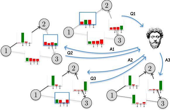
Figure 1: Human-in-the-loop probabilistic CD. We first train an AGFN to fit a data-informed belief over AGs. Then, we iteratively refine it by 1) questioning (Q) experts on the relation between a highly informative pair of variables and 2) updating the belief given the potentially noisy answers (A). The histograms on top of the edges show marginals over edge types (green denotes ground truth). Notably, our belief increasingly concentrates on the true AG, $1\rightarrow 2\leftrightarrow 3$.

This work focuses on recovering the structure of the underlying causal diagram when unobserved confounders may be at play. We propose to address this task by not only leveraging observational data but also by accounting for potentially noisy pieces of expert knowledge, otherwise unavailable as data. Throughout this work, we consider ancestral graphs (AGs) as surrogates for causal diagrams. AGs are particularly convenient since they encode latent confounding without explicitly invoking unobserved variables. Moreover, AGs capture all conditional independencies and ancestral relations among observed variables $\mathbf{V}$, as entailed by a causal diagram (Richardson and Spirtes, 2002).

In the realm of CD from solely observational data, algorithms aim to construct a compact representation of the joint observational distribution $P(\mathbf{V})$, which implies a factorization as a product of conditional probabilities. Notably, multiple models may entail the same conditional independencies; in such cases, they are denoted as Markov-equivalent. As a result, these algorithms can only reconstruct the class of Markov-equivalent models (AGs), denoted as the Markov Equivalence Class (MEC) and typically represented by a Partial Ancestral Graph (PAG). Importantly, CD beyond the MEC by leveraging domain knowledge presents a critical challenge. Notably, there is no proper characterization of an equivalence class that accounts for knowledge stemming from both humans and data (Wang et al., 2022).

There is a variety of algorithms for CD from observational data, primarily categorized into constraint- and score-based methods. The former uses (in)dependence constraints derived via conditional independence tests to directly construct a PAG representing the MEC. The latter uses a goodness-of-fit score to navigate the space of AGs, selecting an optimum as a representative for the MEC.

Nonetheless, methods within both paradigms suffer from unreliability when data is scarce. Specifically, for the majority of the CD algorithms, formal assurances that the inferred MEC accurately represents the true causal model heavily rely on the so-called faithfulness assumption, which posits that all conditional independencies satisfied by $P(\mathbf{V})$ are entailed by the true causal model (Zhang and Spirtes, 2016). However, this presents a critical challenge in real-world scenarios, as violations of the faithfulness assumption become more prominent when relying on $P(\mathbf{V})$ estimated from limited data Uhler et al. (2012); Andersen (2013); Marx et al. (2021). For constraint-based methods, hypothesis tests may lack the statistical power to detect conditional independencies accurately. These errors may propagate and trigger a chain reaction of erroneous orientations Zhang and Spirtes (2008); Zhalama et al. (2017b); Ng et al. (2021). For score-based methods, although score functions directly measure goodness-of-fit on observational data, small sample sizes can significantly skew the estimates for the population parameters. Consequently, structures deemed score-optimal may not necessarily align with the ground-truth MEC  Ogarrio et al. (2016). A major concern is that the overwhelming majority of CD algorithms produce a single representation of the MEC as output, without quantifying the uncertainty that arises during the learning process Claassen and Heskes (2012); Jabbari et al. (2017). This poses a significant challenge for experts, as it hinders their ability to validate the algorithm’s outcome or gain insights into potential venues for improving inference quality.

To alleviate the lack of uncertainty quantification in CD, we propose sampling AGs from a distribution defined using a score function, which places best-scoring AGs around the mode by design. This effectively provides end-users with samples that reflect the epistemic uncertainty inherent in CD, thus allowing their propagation through downstream causal inferences. In particular, we sample from our belief using Generative Flow Networks (GFlowNets; Bengio et al., 2021a, b), which are generative models known for sampling diverse modes while avoiding the mixing time problem of MCMC methods, and not requiring handcrafted proposals nor accept-reject steps (Bengio et al., 2021a).

Acknowledging the low-data regime as CD’s primary challenge, we also propose actively integrating human feedback in the inferential process. This involves modeling user knowledge on the existence and nature (confounding/ancestral) of the relations and using it to weigh our beliefs over AGs. During our interactions with experts, we probe them about the relation of the pair of variables that optimizes a utility/acquisition function, for which we propose the negative expected cross-entropy between our prior and updated beliefs. Unlike prior strategies, our acquisition avoids the need to estimate the normalizing constant and predictive distribution of our updated belief, as needed for information gain and mutual information, respectively. Notably, we use importance sampling (Marshall, 1954; Geweke, 1989) to update our initial belief with the human feedback, which avoids retraining GFlowNets after each human interaction.

While incorporating expert knowledge into CD has been a long-standing goal (Meek, 1995a; Chen et al., 2016; Li and Beek, 2018; Wang et al., 2022), existing works either rely on strong assumptions (e.g., causal sufficiency) or assume the knowledge is noiseless, aligned with the ground truth  (Andrews, 2020; Wang et al., 2022). Importantly, our work introduces the first iterative CD framework for AGs involving a human in the loop and accommodating potentially noisy feedback, as depicted in Figure 1.

To validate our approach, we conduct experiments using the BIC score, for linear Gaussian causal models. Specifically, we assess: i) our ability to sample from score-based beliefs over AGs, ii) how our samples compare to samples from bootstrapped versions of state-of-the-art (SOTA) methods, and iii) the efficacy of our active knowledge elicitation framework using simulated humans. We observe that our method, Ancestral GFlowNet (AGFN), i) accurately samples from our beliefs over AGs; ii) consistently includes AGs with low structural error among its top-scored samples; and iii) is able to greatly improve performance metrics (i.e., SHD and BIC) when incorporating human in the loop.

In summary, the contributions of our work are:

1. We leverage GFlowNets to introduce AGFN, the first CD algorithm for scenarios under latent confounding that employs fully-probabilistic inference on AGs;

2. We show AGFN accurately learns distributions over AGs, effectively capturing epistemic uncertainty.

3. We propose an experimental design to query potentially noisy expert insights on relationships among pairs of variables that lead to optimal uncertainty reduction.

4. We show how to incorporate expert feedback into AGFN without retraining them from scratch.

2 Background

This section introduces the relevant notation and concepts. We use uppercase letters $V$ to represent a random variable or node in a graph, and boldface uppercase letters $\mathbf{V}$ to represent matrices or sets of random variables or nodes.

Ancestral graphs. Under the assumption of no selection bias, an ancestral graph (AG) $\mathcal{G}$ over $\mathbf{V}$ is a directed graph comprising directed ($\rightarrow$) and bidirected ($\leftrightarrow$) edges Richardson and Spirtes (2002); Zhang (2007). In any directed graph, if a sequence of directed edges, $V_{i}\rightarrow\cdots\rightarrow V_{j}$, connects two nodes $V_{i}$ and $V_{j}$, we refer to this sequence as a directed path. In this case, we also say that $V_{i}$ is an ancestor of $V_{j}$ and denote this relation as $V_{i}\in An(V_{j})$. By definition, any AG $\mathcal{G}$ must further satisfy the following:

1. there is no directed cycle, i.e., if $V_{i}\rightarrow V_{j}$ is in $\mathcal{G}$, then $V_{j}\not\in An(V_{i})$; and

2. there is no almost directed cycle, i.e., if $V_{i}\leftrightarrow V_{j}$ is in $\mathcal{G}$, then $V_{j}\not\in An(V_{i})$ and $V_{i}\not\in An(V_{j})$.

As a probabilistic model, the nodes in an AG represent random variables, directed edges represent ancestral (causal) relationships, and bidirected edges represent associations solely due to latent confounding. For a complete characterization of AGs, refer to Richardson and Spirtes (2002).

Data generating model. We assume that the data-generating model corresponds to a linear Gaussian structural causal model (SCM) (Pearl, 2000) defined by a 4-tuple $\mathcal{M}=\langle\mathbf{V},\mathbf{U},\mathcal{F},P(\mathbf{U})\rangle$, in which $\mathbf{V}=\{V_{1},V_{2},\dots,V_{n}\}$ is a set of $n$ observed random variables and $\mathbf{U}=\{U_{1},U_{2},\dots,U_{n}\}$ is the set of unobserved random variables. Further, let $Pa_{i}\subseteq\mathbf{V}\setminus\{V_{i}\}$ be the set of observed causes (parents) of $V_{i}$, and $U_{i}$ be the set of unobserved causes of $V_{i}$. Then, each structural equation $f_{i}\in\mathcal{F}$ is defined as:

$$V_{i}=\sum_{j:V_{j}\in Pa_{i}}\beta_{ij}V_{j}+U_{i}$$ (1)

with $P(\mathbf{U})$ being a multivariate Gaussian distribution with zero mean and a not necessarily identity covariance matrix $\boldsymbol{\Omega}=(\omega_{ij})_{1\leq i,j\leq n}$ — the error terms $\{U_{i}\}$ are not necessarily mutually independent, implying that the system can be semi-Markovian (i.e., latent confounding may be present).

Consider a lower triangular matrix of structure coefficients $\mathbf{B}=(\beta_{ij})_{1\leq i,j\leq n}$ such that $(\mathbf{I}-\mathbf{B})$ is invertible, and $\beta_{ij}\neq 0$ only if $V_{j}\in Pa_{i}$. Then, the set of structural equations is given in matrix form by

$$\mathbf{V}=\mathbf{B}\mathbf{V}+\mathbf{U}\implies\mathbf{V}=(\mathbf{I}-\mathbf{B})^{-1}\mathbf{U}.$$ (2)

The class of all linear Gaussian SCMs parametrized as

$$\mathcal{N}_{\mathcal{M}}=\{\mathcal{N}(\mathbf{0},\boldsymbol{\Sigma})|\boldsymbol{\Sigma}=(\mathbf{I}-\mathbf{B})^{-1}\boldsymbol{\Omega}(\mathbf{I}-\mathbf{B})^{-\top}\}$$ (3)

is represented by an AG in which, for every $i\neq j$, there is a directed edge $V_{j}\rightarrow V_{i}$ if $\beta_{ij}\neq 0$ and a bidirected edge $V_{j}\leftrightarrow V_{i}$ if $\omega_{ij}\neq 0$ (Richardson and Spirtes, 2002).

Figure 2: Illustration of the generative process of AGs $\{\mathcal{G}_{5},\mathcal{G}_{6},\mathcal{G}_{7}\}$ using GFlowNets. Starting with an empty graph $\mathcal{G}_{0}$, we add edges between variables $\{X_{1},X_{2},X_{3}\}$ according to the action-policy $\pi_{F}$. Solid edges trace trajectories leading to sampled graphs. Dashed lines represent non-realized transitions to terminal state $\square$.

GFlowNets. Generative Flow Networks (GFlowNet; Bengio et al., 2021a, b) are generative models designed to sample from a finite domain $\mathcal{X}$ proportionally to some reward function $R:\mathcal{X}\rightarrow\mathbb{R}_{+}$, which may be parametrized using neural networks. In this work, we define $R$ as a strictly decreasing transformation of the BIC (more details in section 3). GFlowNets also assume there is a compositional nature to the elements $x\in\mathcal{X}$, meaning that they can be built by iteratively acting to modify a base object (i.e., an initial state). For instance, graphs can be built by adding edges to a node skeleton (Deleu et al., 2022) or molecules by adding atoms to an initial structure (Bengio et al., 2021a).

The generative process follows a trajectory of states $s\in\mathcal{S}$ guided by a transition probability $\pi_{F}:\mathcal{S}^{2}\rightarrow[0,1]$. In turn, $\pi_{F}$ is proportional to a foward flow function $F_{\theta}:\mathcal{S}^{2}\rightarrow\mathbb{R}_{+}$, which is parameterized by a neural network $\theta$. Let $\text{Pa}(s^{\prime})$ ($\text{Ch}(s^{\prime})$) be the set of all states which can transition into (directly reached from) $s^{\prime}$. Then, $\pi_{F}$ is defined as

$$\pi_{F}(s^{\prime}|s)=\frac{F_{\theta}(s\rightarrow s^{\prime})}{\sum_{{s^{\prime}\in\text{Ch}(s)}}F_{\theta}(s\rightarrow s^{\prime})}.$$ (4)

The support $\mathcal{X}$ of $R$ is contained within $\mathcal{S}$. There are also two special states in $\mathcal{S}$: an initial state $s_{0}$ and a terminal state $s_{f}$. We start with the initial state $s_{0}$ and transform it to a new valid state $s$ with probability $\pi_{F}(s|s_{0};\theta)$. We keep iterating this procedure until reaching $s_{f}$. States $s$ valid as final samples ($s\in\mathcal{X}$) are known as terminating states and have a positive probability for the transition $s\rightarrow s_{f}$. Figure 2 illustrates this process with $\mathcal{X}$ being the space of AGs. Crucially, the same parameterization $\theta$ is used for all transition probabilities $\pi_{F}(\cdot|s;\theta)$ given any departing state $s$, allowing for generalization to states never visited during training.

As the GFlowNet framework requires that no sequence of actions leads to a loop, we represent the space of possible action sequences by a pointed Directed Acyclic Graph (DAG) (Bengio et al., 2021b). The generation of any sample $x\in\mathcal{X}$ follows a trajectory $\tau=(s_{0},s_{1},\ldots,s_{T}=x,s_{f})\in\mathcal{S}^{T+2}$ for a $T\geq 0$. Different trajectories may lead to the same sample $x$. To ensure we sample proportionally to $R$, we search for a GFlowNet that satisfies the flow-matching condition, i.e., $\forall s^{\prime}\in\mathcal{S}$:

$$\sum_{s\in\text{Pa}(s^{\prime})}F_{\theta}(s\rightarrow s^{\prime})=R(s^{\prime})+\sum_{s^{\prime\prime}\in\text{Ch}(s^{\prime})}F_{\theta}(s^{\prime}\rightarrow s^{\prime\prime}).$$ (5)

Equation 5 implies the flow that enters $s^{\prime}$ equals the flow leaving $s^{\prime}$, except for some flow $R(s^{\prime})$ leaking from $s^{\prime}$ into $s_{f}$. We let $R(s)=0$ for $s\notin\mathcal{X}$. Eventually, it may be that all states $s$ are valid candidates, i.e., $\mathcal{S}=\mathcal{X}\cup\{s_{f}\}$. If so, each of eq. 5’s solutions satisfies a detailed-balance condition,

$$\frac{R(s)F_{\theta}(s\rightarrow s^{\prime})F_{\theta}(s^{\prime}\rightarrow s_{f})}{F_{\theta}(s\rightarrow s_{f})}=R(s^{\prime})F_{B,\theta}(s^{\prime}\rightarrow s),$$ (6)

for a parametrized backward flow $F_{B,\theta}\colon\mathcal{S}^{2}\rightarrow\mathbb{R}_{+}$ Deleu et al. (2022). In practice, we enforce eq. 6 by minimizing

$$\mathcal{L}(\theta)\!=\!\underset{s\rightarrow s^{\prime}}{\mathbb{E}}\!\left[\!\left(\!\log\frac{R(s^{\prime})\pi_{F_{B}}(s|s^{\prime};\theta)\pi_{F}(s_{f}|s;\theta)}{R(s)\pi_{F}(s^{\prime}|s;\theta)\pi_{F}(s_{f}|s^{\prime};\theta)}\!\right)^{2}\!\right].$$ (7)

3 Ancestral GFlowNets

We propose AGFN, a GFlowNet-based method for sampling AGs using a score function. Specifically, AGFN encompasses a GFlowNet with the following characteristics:

1. Each trajectory state is a valid AG $\mathcal{G}_{t}$.

2. A terminating state’s reward $R(\mathcal{G_{T}})$ is a score-based potential suitable for CD of AGs.

3. A well-trained AGFN samples AGs with frequencies proportional to their rewards and with the best-scoring AG being, by design, the mode.

The generation of a trajectory $\tau=\{\{\},\mathcal{G}_{1},\mathcal{G}_{2},\ldots,\mathcal{G}_{T}\}$ begins with a totally disconnected graph with nodes $\mathbf{V}$, iteratively adding edges of types $\{\leftarrow,\rightarrow,\leftrightarrow\}$ between pairs of variables. The following paragraphs describe AGFN. For further details, please refer to the Appendix.

Action constraints. To ensure AGFN only samples AGs, we mask out actions that would lead to paths forming cycles or almost cycles. To achieve this, we verify whether the resulting graph respects Bhattacharya et al. (2021)’s algebraic characterization of the space of AGs. More specifically, any AG $\mathcal{G}$ is characterized by an adjacency matrix $\mathbf{A}_{d}\in\mathbb{R}^{n\times n}$ for its directed edges and another adjacency matrix $\mathbf{A}_{b}\in\mathbb{R}^{n\times n}$ for its bidirected edges, adhering to:

$$\text{trace}(\exp\{\mathbf{A}_{d}\})-n+\mathbf{1}^{T}(\exp\{\mathbf{A}_{d}\}\odot\mathbf{A}_{b})\mathbf{1}=0,$$ (8)

in which $\mathbf{1}$ is a $n$-dimensional unit vector and $\odot$ denotes the Hadamard (elementwise) product of matrices.

Score-based belief. We propose using a strictly decreasing transformation of a score function $U$ as the reward $R$ for AGFN. More precisely, we define $R$ as

$$R(\mathcal{G})=\exp\left\{\frac{\mu-U(\mathcal{G})}{\sigma}\right\}$$ (9)

for given constants $\mu\in\mathbb{R}$ and $\sigma\in\mathbb{R}^{+}$ that ensure numerical stability (Zhang et al., 2023). In practice, we sample $S$ AGs $\{\mathcal{G}^{(s)}\}_{s=1}^{S}$ from an untrained AGFN, and set $\mu=\nicefrac{{1}}{{S}}\sum_{s}U(\mathcal{G}^{(s)})$ and $\sigma=\sqrt{\nicefrac{{1}}{{S}}\sum_{s}(U(\mathcal{G}^{(s)})-\mu)^{2}}$.

Score for linear Gaussian models. Since we focus on linear Gaussian models, we choose the extended Bayesian Information Criterion Foygel and Drton (2010) as our score function. Specifically, for any AG $\mathcal{G}=(\mathbf{V},\mathbf{E})$:

$$U(\mathcal{G}) =-2l_{N}(\hat{\mathbf{B}},\hat{\boldsymbol{\Omega}})+|\mathbf{E}|\log n+2|\mathbf{E}|\log|\mathbf{V}|,$$ (10)

in which $(\hat{\mathbf{B}},\hat{\boldsymbol{\Omega}})$ is the MLE estimate of model parameters (see eq. 3) obtained using the residual iterative conditional fitting algorithm Drton et al. (2009).

Forward flow. We use a Graph Isomorphism Network (GIN) Xu et al. (2019) $\Phi$ to compute a $d$-dimensional representation for each node in the AG $\mathcal{G}_{t}$ at the $t$-th step of the generative process and use sum pooling to get an embedding for $\mathcal{G}_{t}$. Then, considering $\mathcal{A}_{t}$ as the space of feasible actions at $\mathcal{G}_{t}$ (i.e., those leading to an AG), we use an MLP $\phi\colon\mathbb{R}^{d}\rightarrow\mathbb{R}^{|\mathcal{A}_{t}|}$ with a softmax activation at its last layer to map $\mathcal{G}_{t}$’s embedding to a distribution over $\mathcal{A}_{t}$. More precisely, given $\mathbf{H}^{(t)}=\Phi(\mathcal{G}_{t})\in\mathbb{R}^{|\mathbf{V}|\times d}$, we compute

$$\mathbf{p}=\phi\left(\sum_{v\in\mathbf{V}}\mathbf{H}_{v}^{(t)}\right)$$ (11)

as the probability distribution over the feasible actions at $\mathcal{G}_{t}$.

Backward flow. Backward actions correspond to removing edges. Following Shen et al. (2023), we parametrize the backward flow $F_{B}$ with an MLP and alternate between updating $\pi_{F}$ and $\pi_{F_{B}}$, using gradient-based optimization.

4 Human-in-the-Loop Causal Discovery

Concluding the training, we propose leveraging the AGFN-generated samples to design questions for the expert that optimize the reduction of entropy in the distribution $p_{\theta}(\mathcal{G})$ over the space of AGs. Then, we use the human feedback to update $p_{\theta}(\mathcal{G})$, and iteratively repeat the process. The following paragraphs describe i) how we model human feedback, ii) how we update our belief over AGs given human responses, and iii) our experimental design strategy for expert inquiry.

Modeling human feedback.

We assume humans are capable of answering questions regarding the ancestral relationship between pairs of random variables. In this case, we model their prior knowledge on a relation $r=\{U,V\}$ between nodes $U,V\in\mathbf{V}$ as a categorical distribution over a random variable denoted $\omega_{r}$. Fix an arbitrary total order $<$ in $\mathbf{V}$. By definition, $\omega_{r}=1$ if there is no edge between $U$ and $V$; $\omega_{r}=2$ if $U$ is ancestor of $V<U$; $\omega_{r}=3$ if $V$ is ancestor of $U>V$; and $\omega_{r}=4$ if there is a bidirected edge between $U$ and $V$. Since the human has access to our AGFN before being probed for the first time, we set $\rho_{r,k}=p_{\theta}(\omega_{r}=k)$ as the prior probability of $\omega_{r}=k$. Moreover, we consider that the expert’s feedback $f_{r}\in\{1,2,3,4\}$ on the relation $r$ is a noisy realization of the true, unobserved value of the relation feature $\omega_{r}$ under the expert’s model. Putting all elements together results in a two-level Bayesian hierarchical scheme for categorical data:

$$\omega_{r} \sim\text{Cat}(\boldsymbol{\rho}_{r}),$$ (12)

$$f_{r}|\omega_{r} \sim\text{Cat}\left(\delta_{\omega_{r}}\cdot\pi+(\mathbf{1}-\delta_{\omega_{r}})\cdot\left(\frac{1-\pi}{3}\right)\right),$$ (13)

in which $\boldsymbol{\rho}_{r}=(\rho_{r,1},\rho_{r,2},\rho_{r,3},\rho_{r,4})$ represents our prior beliefs about the relations’ features, $\pi\in[0,1]$ reflects the reliability of the expert’s feedback, and $\delta_{k}$ is the $k$-th canonical basis of $\mathbb{R}^{4}$. Conveniently, the posterior distribution of the relation feature $\omega_{r}$ given the feedback $f_{r}$ is a categorical distribution parametrized by

$$\frac{\boldsymbol{\rho}_{r}}{\eta_{r}}\odot\left(\pi\cdot\delta_{f_{r}}+\left(\frac{1-\pi}{3}\right)\cdot(\mathbf{1}-\delta_{f_{r}})\right),$$ (14)

with $\eta_{r}=\rho_{r,f_{r}}\cdot\pi+\left(\frac{1-\pi}{3}\right)\cdot(1-\rho_{r,f_{r}})$.

Figure 3: Sampling quality. The reward-induced marginal distribution over graph features is adequately approximated by the marginal distribution learned by the GFlowNet.

Updating beliefs.

We update our AGFN by weighing it by our posterior over the expert’s knowledge, described in the previous paragraph, similarly to a product-of-experts approach Hinton (2002). For this, let $\mathbf{f}_{K}=(f_{r_{k}})_{1\leq k\leq K}$ be the sequence of $K$ feedbacks issued by the expert and define our novel belief distribution $q(\mathcal{G};\mathbf{f}_{K})$ over the space of AGs as

$$q(\mathcal{G};\mathbf{f}_{K})\propto p_{\theta}(\mathcal{G})\prod_{1\leq k\leq K}p(\omega_{r_{k}}|f_{r_{k}}).$$ (15)

Importantly, we use $p_{\theta}$ as proposal distribution in importance (re-)sampling Gordon et al. (1993) to approximately sample from $q(\mathcal{G};\mathbf{f}_{K})$ — or to approximate the expected value of a test function. More precisely, we estimate the value of a function $h$ over the space of AGs as:

$$\mathbb{E}_{q}[h(\mathcal{G})]\approx\sum_{t=1}^{T}c^{-1}\frac{q(\mathcal{G}^{(t)};\mathbf{f}_{K})}{p_{\theta}(\mathcal{G}^{(t)})}h(\mathcal{G}^{(t)})$$ (16)

with $(\mathcal{G}^{(t)})_{t=1}^{T}\sim p_{\theta}(\mathcal{G})$ and $c=\sum_{t=1}^{T}\nicefrac{{q(\mathcal{G}^{(t)};\mathbf{f}_{K})}}{{p_{\theta}(\mathcal{G}^{(t)})}}$.

Active knowledge elicitation.

To make the most out of possibly costly human interactions, we query the human about the relation that maximally reduces the expected cross-entropy between our belief over AGs before and after human feedback. More precisely, we define an acquisition function $a_{k}:{{\mathbf{V}}\choose{2}}\rightarrow\mathbb{R}$ for the $k>1$-th inquiry as:

$$a_{k}(r)=-\mathbb{E}_{f_{r}\sim p(\cdot|\mathbf{f}_{K})}\big{[}\mathbf{H}\left(q(\mathcal{G};\mathbf{f}_{K},f_{r}),q(\mathcal{G};\mathbf{f}_{K})\right)\!\big{]}$$ (17)

in which $p(f_{r}|\mathbf{f}_{K})$ is the posterior predictive distribution according to the user model, $q_{0}\propto R$ and $\mathbf{H}(\cdot,\cdot)$ is the cross-entropy. Then, we maximize this acquisition to select which relation $\tilde{r}_{k}$ we will probe the expert, i.e.:

$$\tilde{r}_{k}=\operatorname*{arg\ max}_{r\in{{\mathbf{V}}\choose{2}}}a_{k}(r).$$ (18)

As aforementioned, we use importance sampling with $q_{0}$ as a proposal to estimate the acquisition function $a_{k}$. This allows us to leverage AGFN samples and effectively avoid the need for retraining them. It is worth mentioning that because $\mathbf{H}(p,p^{\prime})\geq\mathbf{H}(p,p)$ for any two distributions $p$ and $p^{\prime}$ of the same support, our strategy is equivalent to minimizing an upper bound on the entropy of $q_{k}$. Also, different from acquisitions based on information gain or mutual information, approximating Equation 17 via Monte Carlo does not require exhaustive integration over the space of AGs to yield asymptotically unbiased estimates — see Appendix.

	chain4		IV		collfork
	SHD	BIC	SHD	BIC	SHD	BIC
FCI⋆	$3.03{\color[rgb]{.5,.5,.5}}$	$5481.33{\color[rgb]{.5,.5,.5}}$	$\mathbf{3.75}{\color[rgb]{.5,.5,.5}}$	$\mathbf{5426.18}{\color[rgb]{.5,.5,.5}}$	$6.26{\color[rgb]{.5,.5,.5}}$	$5433.80{\color[rgb]{.5,.5,.5}}$
GFCI⋆	$\mathbf{2.24}{\color[rgb]{.5,.5,.5}}$	$\mathbf{5479.77}{\color[rgb]{.5,.5,.5}}$	$4.21{\color[rgb]{.5,.5,.5}}$	$5427.09{\color[rgb]{.5,.5,.5}}$	$\mathbf{5.23}{\color[rgb]{.5,.5,.5}}$	$\mathbf{5431.67}{\color[rgb]{.5,.5,.5}}$
DCD⋆	$3.38{\color[rgb]{.5,.5,.5}}$	$5482.97{\color[rgb]{.5,.5,.5}}$	$5.22{\color[rgb]{.5,.5,.5}}$	$5429.51{\color[rgb]{.5,.5,.5}}$	$6.02{\color[rgb]{.5,.5,.5}}$	$5436.84{\color[rgb]{.5,.5,.5}}$
N-ADMG	$6.14{\color[rgb]{.5,.5,.5}}$	$5520.01{\color[rgb]{.5,.5,.5}}$	$\mathbf{8.50}{\color[rgb]{.5,.5,.5}}$	$5583.17{\color[rgb]{.5,.5,.5}}$	$7.16{\color[rgb]{.5,.5,.5}}$	$5491.86{\color[rgb]{.5,.5,.5}}$
AGFN (ours)	$\mathbf{6.04}{\color[rgb]{.5,.5,.5}}$	$\mathbf{5494.67}{\color[rgb]{.5,.5,.5}}$	$8.72{\color[rgb]{.5,.5,.5}}$	$\mathbf{5456.16}{\color[rgb]{.5,.5,.5}}$	$\mathbf{6.58}{\color[rgb]{.5,.5,.5}}$	$\mathbf{5478.01}{\color[rgb]{.5,.5,.5}}$

Table 1: Average SHD and BIC. The ^⋆ denotes methods yielding point estimates. We use Bootstrap to report the mean and average standard deviation for these. For N-ADMG and AGFN, we estimate the quantities using $100$k samples.

5 Experiments

Our experiments have three objectives. First, we validate that AGFN can accurately learn the target distribution over the space of AGs. Second, we show that AGFN performs competitively with alternative methods on three data sets. Third, we attest that our experimental design for incorporating the expert’s feedback efficiently reduces the uncertainty over AGFN’s distribution. We provide further experimental details in the Appendix. Code is available in the supplement.

5.1 Distributional Assessment of AGFN

Data. Since violations of faithfulness are more likely in dense graphs Uhler et al. (2012), we create $20$ $5$-node random graphs Uhler et al. (2012) from a directed configuration model (Newman, 2010) whose in- and out-degrees are uniformly sampled from $\{0,1,2,3,4\}$. We draw $500$ independent samples from a structure-compatible linear Gaussian SCM with random parameters for each graph.

Setup. We train AGFN for each random graph using their respective samples. Then, we collect AGFN samples and use them to compute empirical distributions over the (i) edge features (i.e., $p_{\theta}(U\rightarrow V)$, $p_{\theta}(U\leftarrow V)$, $p_{\theta}(U\leftrightarrow V)$ and $p_{\theta}(U\not\mathrel{-}V)$ for each pair $(U,V)$), (ii) BIC, and (iii) structural Hamming distance to the true causal diagram (SHD).

Results. Figure 3 shows that the AGFN adequately approximates the theoretical distribution induced by the reward in Equation 9. Furthermore, AGFNs induce distributions over BIC and SHD values that closely resemble those induced by $p(\mathcal{G})\propto R(\mathcal{G})$. We also note an important improvement over the prior art on probabilistic CD (N-ADMG): we found that over $60\%$ of its samples were non-ancestral and that this method was of little use for making inferences over AGs. Meanwhile, AGFN does not sample non-ancestral graphs.

5.2 Comparison with SOTA CD algorithms

(a) chain4

(b) IV

(c) collfork

Figure 4: Ancestral graphs representing the data generating models for the three considered datasets in Table 1.

Data. We generate $10$ datasets with $500$ independent samples from the randomly parametrized linear Gaussian SCMs corresponding to the canonical causal diagram Richardson and Spirtes (2002) in each AG depicted in Figure 4. Unshielded colliders and discriminating paths are fundamental patterns in the detection of invariances by CD algorithms under latent confounding Spirtes and Richardson (1997); Zhang (2008b). Thus, we consider the following 4-node causal diagrams with increasingly difficult configurations: (i) chain4, a chain without latent confounders; (ii) collfork, a graph with triplets involving colliders and non-colliders under latent confounding, and (iii) IV, a structure with a discriminating path for $Z$: $W\rightarrow X\leftarrow Z\rightarrow Y$.

Baselines. We compare AGFN with four notable CD methods: FCI (Spirtes et al., 2001; Zhang, 2008b), GFCI (Ogarrio et al., 2016), DCD (Bhattacharya et al., 2021), and N-ADMG Ashman et al. (2023). The baselines span four broad classes of CD methods. FCI is a seminal constraint-based CD algorithm that learns a PAG consistent with conditional independencies entailed by statistical tests. GFCI is a hybrid CD algorithm that learns a PAG by first obtaining an approximate structure using FGS (Ramsey, 2015) (a BIC-score-based search algorithm for causally sufficient scenarios) and then by applying FCI to identify possible confounding and remove some edges added by FGS. DCD casts CD as continuous optimization with differentiable algebraic constraints defining the space of AGs and uses gradient-based algorithms to solve it. N-ADMG computes a variational approximation of the joint posterior distribution over the space of bow-free causal diagrams (Nowzohour et al., 2017) associated with non-linear SCMs with additive noise. While N-ADMG focuses on a more restricted setting compared to AGs, it offers some uncertainty quantification in the variational pohttps://www.overleaf.com/project/650454a084b798332af29ebesterior, making it more closely comparable to our approach. We rigorously follow the experimental guidelines in the original works.

Experimental setup We train AGFN on each dataset and use it to sample 100k graphs. We also apply FCI, GFCI, and DCD to $100$ bootstrapped resamplings of each dataset to emulate confidence distributions induced by these algorithms. To compare the algorithms’ outputs, we compute the sample mean and standard deviation of the BIC and SHD at the PAG level. Specifically, we compute the SHD between the ground-truth PAG and each estimated PAG obtained by each method. If the output is a PAG member (as for DCD, N-ADMG, and AGFN) we use FCI to transform the output using these graphs as oracles for conditional independencies. Furthermore, we directly compute the BIC for the outputs, as all PAG members are asymptotically score-equivalent.

Results. Table 1 compares AGFN against baseline CD algorithms. Notably, our method consistently outperforms the only probabilistic baseline in the literature (N-ADMG) in terms of both SHD and BIC. As expected, however, the average BIC and SHD induced by AGFN are larger than those induced by the bootstrapped versions of the non-probabilistic algorithms, and the variances are greater; this is due to the inherent sampling diversity of our method and the resulting generation of possibly implausible samples. Indeed, Table 2 shows that the three most rewarding samples from AGFN are as good as (and sometimes better than) the other CD algorithms. Results for N-ADMG comprise the three most frequent samples from the variational distribution.

	chain4	IV	collfork
FCI	$2.07{\color[rgb]{.5,.5,.5}}$	$3.83{\color[rgb]{.5,.5,.5}}$	$5.43{\color[rgb]{.5,.5,.5}}$
GFCI	$\mathbf{1.50}{\color[rgb]{.5,.5,.5}}$	$3.63{\color[rgb]{.5,.5,.5}}$	$5.53{\color[rgb]{.5,.5,.5}}$
DCD	$2.27{\color[rgb]{.5,.5,.5}}$	$4.80{\color[rgb]{.5,.5,.5}}$	$5.60{\color[rgb]{.5,.5,.5}}$
N-ADMG (top 3)	$4.38{\color[rgb]{.5,.5,.5}}$	$6.08{\color[rgb]{.5,.5,.5}}$	$6.87{\color[rgb]{.5,.5,.5}}$
AGFN (top 3)	$2.00{\color[rgb]{.5,.5,.5}}$	$\mathbf{3.50}{\color[rgb]{.5,.5,.5}}$	$\mathbf{4.90}{\color[rgb]{.5,.5,.5}}$

Table 2: SHD for point estimates. The mean SHD of the top-3 AGFN draws is comparable to or better than baselines.

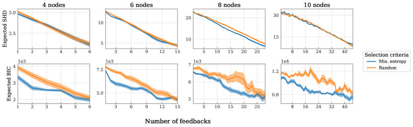
Figure 5: CD with simulated human feedback. The top/bottom row shows the mean SHD/BIC of AGFN samples as a function of human interactions. Probing the expert about the edge that minimizes the mean cross-entropy leads to a faster decrease in BIC compared to a random strategy. The SHD decreases similarly in both cases. Results reflect the outcomes of 30 simulations.

5.3 Simulating humans in the loop

Data. We follow the procedure from Section 5.1 to generate graphs with $4$, $6$, $8$ and $10$ nodes. We draw $500$ samples from a compatible linear Gaussian SCM and use them to train an AGFN. Then, we follow our active elicitation strategy from Section 4 to probe simulated humans, adhering to the generative model described in the same section, with $\pi=0.9$.

Setup. Since we are the first to propose an optimal design for expert knowledge elicitation, there are no baselines to compare AGFN against. That being said, we aim to determine whether the inclusion of expert feedback enhances the concentration of the learned distribution around the true AG, and evaluate the effectiveness of our elicitation strategy. To do so, we measure SHD to the true AG and BIC as a function of the number of expert interactions.

Results. Figure 5 shows that incorporating expert feedback substantially decreases the expected SHD and BIC under our belief over AGs. On the one hand, the remarkable decrease in expected SHD shows that our belief becomes increasingly focused on the true AG as we iteratively request the expert’s feedback, regardless of the querying strategy. On the other hand, the second row shows that our querying strategy results in a substantial decrease in the BIC, demonstrating a faster reduction than random queries. This validates the notion that some edges are more informative than others, and we should prioritize them when probing the expert.

6 Related Work

CD under latent confounding. Following the seminal works by Spirtes et al. (2001) and Zhang (2008b) introducing the complete FCI, a variety of works have emerged. Among them are algorithms designed for sparse scenarios, including RFCI (Colombo et al., 2012) and others (Silva, 2013; Claassen et al., 2013). Notably, Silva (2013)’s framework uses a Bayesian approach to CD of Gaussian causal diagrams based on sparse covariance matrices. Nonetheless, it requires sampling one edge at a time and relies on numerical heuristics that might effectively alter the posterior we are sampling from. Colombo et al. (2012) introduced the conservative FCI to handle conflicts arising from statistical errors in scenarios with limited data, even though it yields less informative results. Subsequent efforts to improve reliability led to the emergence of constraint-based CD algorithms based in Boolean satisfiability (Hyttinen et al., 2014; Magliacane et al., 2016), although they are known to scale poorly on $|\mathbf{V}|$ (Lu et al., 2021). In another paradigm, score-based search algorithms rank MAGs according to goodness-of-fit measures, commonly using BIC for linear Gaussian SCMs (Triantafillou and Tsamardinos, 2016; Zhalama et al., 2017a; Rantanen et al., 2021). There are also hybrid approaches that combine constraint-based strategies to reduce the search space, such as GFCI (Ogarrio et al., 2016), M3HC (Tsirlis et al., 2018), BCCD (Claassen and Heskes, 2012), and GSPo (Bernstein et al., 2020). Continuous optimization approaches have recently emerged as a novel approach to score-based CD, such as DCD (Bhattacharya et al., 2021) and N-ADMG Ashman et al. (2023).

CD with expert knowledge. Previous works on CD have explored various forms of background knowledge. This includes knowledge on edge existence/non-existence Meek (1995b), ancestral constraints Chen et al. (2016), variable grouping Parviainen and Kaski (2017), partial order Andrews (2020) and typing of variables (Brouillard et al., 2022). Incorporating expert knowledge is pivotal to reducing the search space and the size of the learned equivalence class. However, due to significant challenges, up to date, there are only a few works trying to integrate human knowledge into CD within the context of latent confounding (Andrews, 2020; Wang et al., 2022). These works operate under the assumption of perfect expert feedback. In contrast, our contribution is novel in that it confronts the challenges of real-world situations where expert input might be inaccurate.

7 Discussion

We presented AGFN, the first probabilistic CD method that accounts for latent confounding and incorporates potentially noisy human feedback in the loop. AGFN samples AGs according to a score function, quantifying the uncertainty in the learning process. Furthermore, it can leverage human feedback in an optimal design strategy, efficiently reducing our uncertainty on the true data-generating model.

This work is focused on linear Gaussian models, using BIC as our score. However, the implementation of AGFNs is not restricted by this choice. In principle, we could replace the BIC with alternative score functions that are more appropriate for different types of variables, e.g. for discrete data (Drton and Richardson, 2008). It is also important to highlight that our framework does not require retraining the AGFN after we see human feedback. Moreover, AGFN is a GPU-powered algorithm, and while we used only one GPU in our experiments, it is possible to greatly accelerate AGFN by using cluster architectures with multiple GPUs.

By offering uncertainty-quantified CD together with a recipe for including humans in the loop, we expect AGFNs will significantly enhance the accuracy and reliability of CD, especially in real-world domains. Moreover, AGFNs bring a novel perspective to developing more comprehensive tools for downstream causal tasks Bareinboim and Pearl (2016), as the resulting distribution encodes knowledge from data and human feedback while accounting for epistemic uncertainty. For example, methods for causal reasoning that currently rely on a single AG Zhang (2008a); Jaber et al. (2022) could exploit this distribution to incorporate a richer understanding of uncertainty and knowledge, thereby enhancing their robustness and reliability.

Appendix A Additional Related Works

Generative Flow Networks (GFlowNets; Bengio et al., 2021a, b) are generative models that sample discrete composite objects from an unnormalized reward function. They have been successfully used to sample various structures such as protein sequences (Jain et al., 2022) and schedules (Zhang et al., 2023). They have also been used to train energy-based models (Zhang et al., 2022). In the field of structure learning, they have been applied to Bayesian networks — more specifically to sample a posterior over DAGs in linear Gaussian networks, although without accounting for unobserved confounding (Deleu et al., 2022). Recently, Deleu et al. (2023) proposed an extension to jointly infer the structure and parameters, also grounded in the assumption of causal sufficiency. It is worth highlighting that training GFlowNets in these scenarios presents optimization challenges, resulting in the utilization of a variety of loss functions (Shen et al., 2023). Moreover, Lahlou et al. (2023) proposed an extension of GFlowNets to continuous domains.

Appendix B Cross-entropy acquisition

The expected mutual information and the information gain are the most widely used information-theoretic measures to actively interact with a human and choose the most informative data points to be labeled Ryan et al. (2015). However, we instead use the negative expected cross-entropy between the current and updated beliefs as the acquisition function of our experimental design (see eq. 17). As we show next, the approximation of both the mutual information and the information gain is intrinsically dependent upon the estimation of the log-partition of the updated beliefs over the space of ancestral graphs. Doing so is computationally intensive, and we would either need to use a Monte Carlo estimator of the integrals or use some posterior approximation — in both cases, leading to asymptotically biased estimates of the acquisition. In contrast, we can easily leverage AGFN samples to compute asymptotically unbiased estimates of our acquisition function. The next paragraphs provide further details.

Mutual information.

The mutual information between two random variables $X$ and $Y$ with joint distribution $p(X,Y)$ and marginal distributions $p(X)$ and $p(Y)$ is

$$I(X,Y)=\mathcal{D}_{KL}[p(X,Y)||p(X)\otimes p(Y)],$$ (19)

in which $\mathcal{D}_{KL}$ is the Kullback-Leibler divergence. In this context, an alternative approach to our experimental design for active knowledge elicitation would consist in iteratively maximizing the expected mutual information between the observed samples, $\mathcal{G}$, and the elicited feedback, $f_{K}$, to select the relation about which the expert would provide feedback. More specifically, we could choose

$$r_{K+1}=\operatorname*{arg\ max}_{r\in{\mathbf{V}\choose 2}}\mathbb{E}_{f_{r}\sim p(\cdot|\mathbf{f}_{K})}[I(\mathcal{G},f_{r})],$$ (20)

in which

$$I(\mathcal{G},f_{r})=\mathcal{D}_{KL}[q(\mathcal{G},f_{r}|\mathbf{f}_{K})||q(\mathcal{G}|\mathbf{f}_{K})\otimes p(f_{r}|\mathbf{f}_{K})],$$ (21)

at each interaction with the expert. Nonetheless, note that

$$q(\mathcal{G},f_{r}|\mathbf{f}_{K})=q(\mathcal{G}|\mathbf{f}_{K+1})p(f_{r}|\mathbf{f}_{K})$$

$$=c_{K+1}(f_{r})p_{\theta}(\mathcal{G})\left(\prod_{1\leq k\leq K+1}p(\omega_{r_{k}}|f_{r_{k}})\right)\cdot p(f_{r}|\mathbf{f}_{K}),$$

with $f_{r_{K+1}}=f_{r}$ and

$$c_{K+1}(f_{r})=\left(\!\!\sum_{\mathcal{G}}p_{\theta}(\mathcal{G})\!\!\left(\prod_{1\leq k\leq K+1}p(\omega_{r_{k}}|f_{r_{k}})\!\!\right)\!\!\right)^{-1}$$ (22)

as the partition function of our updated beliefs. Note also that Equation 21 entails computing the entropy of $q(\mathcal{G},f_{r}|\mathbf{f}_{K})$. Thus, the selection criterion in eq. 20 requires an accurate estimate of $\log c_{K+1}(f_{r})$ — which is well-known for being a difficult problem Ma et al. (2013) — and the Monte Carlo estimator for the log-partition function is asymptotically biased.

Information gain.

The expected information gain of an elicitation is defined as the expected KL divergence between our updated and current beliefs over ancestral graphs. This approach is widely employed in Bayesian experimental design Ryan et al. (2015). In our framework, the information gain resulting from a feedback $f_{r}$ is

$$\text{IG}_{K}(f_{r})=\mathcal{D}_{KL}[q(\mathcal{G}|\mathbf{f}_{K}\cup f_{r})||q(\mathcal{G}|\mathbf{f}_{K})],$$ (23)

which yields the criterion

$$r_{K+1}=\operatorname*{arg\ max}_{r\in{\mathbf{V}\choose 2}}\mathbb{E}_{f_{r}\sim p(\cdot|\mathbf{f}_{K})}\left[\text{IG}_{K}(f_{r})\right].$$ (24)

Nonetheless, eq. 24 suffers from the same problems of eq. 20: it requires approximating the logarithm of the partition function $c_{K+1}(f_{r})$ of a distribution over the combinatorially large space of ancestral graphs, which is notably very challenging to estimate. Indeed, as

$$\mathcal{D}_{KL}[q(\mathcal{G}|\mathbf{f}_{K+1})||q(\mathcal{G}|\mathbf{f}_{K})]=\underset{\mathcal{G}\sim q(\cdot|\mathbf{f}_{K+1})}{\mathbb{E}}\left[\log\frac{q(\mathcal{G}|\mathbf{f}_{K+1})}{q(\mathcal{G}|\mathbf{f}_{K})}\right]$$

$$=\underset{\mathcal{G}\sim q(\cdot|\mathbf{f}_{K+1})}{\mathbb{E}}\left[\log p(f_{r}|\omega_{r})+\log c_{K+1}(f_{r})-\log c_{K}\right],$$

with $f_{r_{K+1}}=f_{r}$, $c_{K}$ as the partition function of $q(\cdot|\mathbf{f}_{K})$ — that does not depend upon $f_{r}$ —, and $c_{K+1}(f_{r})$ defined in eq. 22, the estimation of the information gain is inherently dependent upon the estimation of the log-partition function.

Cross-entropy.

The cross-entropy between our updated and current beliefs is an intuitively plausible and practically useful strategy to interact with an expert efficiently. In fact, since

$$\begin{split}\mathbf{H}&[q(\cdot|\mathbf{f}_{K+1}),q(\cdot|\mathbf{f}_{K})]\\ &=\underset{\mathcal{G}\sim q(\cdot|\mathbf{f}_{K+1})}{\mathbb{E}}[-\log q(\mathcal{G}|\mathbf{f}_{K})]\\ &=\underset{\mathcal{G}\sim q(\cdot|\mathbf{f}_{K+1})}{\mathbb{E}}\left[-\log p_{\theta}(\mathcal{G})-\sum_{1\leq k\leq K}\log p(\omega_{r_{k}}|f_{r_{k}})-l_{K}\right]\end{split},$$

in which $l_{K}$ is the log-partition function of the distribution $q(\cdot|\mathbf{f}_{K})$. Further, the cross-entropy depends exclusively upon i) the logarithm of the samples’ rewards, $\log p_{\theta}(\mathcal{G})$, which is readily computed within AGFN’s generative process, and ii) the posterior distribution over the relations’ features $\omega_{r}$ given the expert’s feedbacks $f_{r}$, which is available in closed form. Hence, the previously mentioned expectation is unbiasedly and consistently estimated by our importance sampling scheme. Furthermore, our empirical findings in fig. 5 suggest that the cross-entropy yields good results and consistently outperforms a uniformly random strategy with respect to the BIC score.

Appendix C Experimental details

We lay out the experimental and implementational details of our empirical analysis in the next subsections. In Section C.1, we describe the specific configurations of the CD algorithms that we compared with our method in table 2. Then, we consider in section C.2 some practical guidelines and architectural specifications that enable us to train and make inferences with AGFN efficiently. Finally, we contemplate in section C.3 the algorithmic details for simulating the expert’s feedback according to our model for active knowledge elicitation.

C.1 Baselines

FCI.

For the results in table 1, we first estimated a PAG using the stable version of FCI, which produces a fully order-independent final skeleton (Colombo et al., 2014). To identify conditional independencies, we used Fisher’s Z partial correlation test with a significance level of $\alpha=0.05$. The BIC score associated with the PAG estimated by the FCI was computed as the BIC of a randomly selected maximal AG (MAG) within the equivalence class characterized by such PAG. The maximality of an AG depends on the absence of inducing paths between non-adjacent variables, which are paths where every node along it (except the endpoints) is a collider and every collider is an ancestor of an endpoint (Rantanen et al., 2021). This ensures that in the MAG every non-adjacent pair of nodes is m-separated by some set of other variables. Importantly, Markov equivalent MAGs exhibit asymptotic equivalence in terms of BIC scores (Richardson and Spirtes, 2002). As a result, the choice of a random MAG does not disrupt the validity of our results.

GFCI.

Similarly, we applied GFCI with an initial search algorithm (FGS) based on the BIC score and the subsequent application of the FCI with conditional independencies identified by the Fisher’s Z partial correlation test with a significance level $\alpha=0.05$. This was performed for all datasets listed in table 1. Also similar to the procedure adopted with the FCI, the BIC score associated with the estimated PAG was computed as the BIC of a randomly selected MAG within the equivalence class characterized by such PAG.

DCD.

We adhered to the instructions provided in the official repository to apply the DCD method on the datasets in table 1. The SHD was obtained between the ground-truth PAG and the PAG corresponding to the estimated ADMG (i.e., the one obtained via FCI by using the d-separations entailed by the estimated ADMG as an oracle for conditional independencies). On the other hand, the BIC was computed for the estimated ADMG directly.

N-ADMG.

To estimate the parameters of the variational distribution defined by N-ADMG, we executed the code provided at the official repository For fairness, we used the same hyperparameters and architectures reported in their original work Li et al. (2023); in particular, we trained the models for $30$k epochs. After this, we sampled $100$k graphs from the learned distribution. It is worth mentioning that the constraints of bow-free ADMG are guaranteed in the N-ADMG samples only in an asymptotic sense. Thus, we manually removed any cyclic graphs from the learned distribution. Then, we proceeded exactly as with DCD to estimate both the average SHD and the average BIC under the variational distribution.

C.2 Implementational details for AGFN

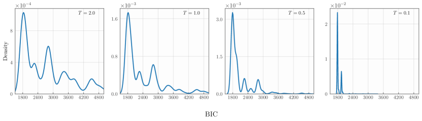
Figure 6: Tempered rewards. Training AGFN to sample from increasingly cold distributions (eq. 25) enables us to increase the proportion of high-scoring graphs (i.e., with a low BIC-score) with the drawback of reducing the AGFN’s sampling diversity.

Masking.

To ensure AGFN only samples ancestral graphs, we keep track of a binary mask $\mathbf{m}_{t}$ that indicates which actions lead to a valid state at the iteration $t$ of the generative process; this mask defines the support of the policy evaluated at the corresponding state. In more detail, let $\mathbf{y}_{t}$ be the last layer embedding (prior to a softmax) at iteration $t$ of the neural network used to parametrize the forward flow of AGFN. The probability distribution over the space of feasible actions is then

$$\mathbf{p}_{t}=\text{Softmax}\left(\mathbf{y}_{t}\odot\mathbf{m}_{t}+\epsilon\cdot(1-\mathbf{m}_{t})\right)$$

for a large and negative constant $\epsilon$. We empirically verified that $\epsilon=-10^{5}$ is sufficient to avoid the sampling of non-ancestral graphs.

Exploratory policy.

During training, we must use an exploratory policy that (i) enables the exploration of yet unvisited states within the pointed DAG and (ii) exploits highly valuable and already visited states. To alleviate this phenomenon, we also draw trajectories from a uniform policy, which is a widespread practice in the literature (Bengio et al., 2021a; Deleu et al., 2022; Shen et al., 2023). More precisely, let $\text{Ch}(\mathcal{G}_{t})$ be the set of states (i.e., ancestral graphs) directly reachable from $\mathcal{G}_{t}$ and $\alpha\in[0,1]$. At each iteration $t$ of the generative process, we sample an action (either an edge to be appended to the graph or a signal to stop the process)

$$a_{t}\sim(1-\alpha)\cdot\mathcal{U}(\text{Ch}(\mathcal{G}_{t}))+\alpha\cdot\pi_{F}(\cdot|\mathcal{G}_{t})$$

and modify $\mathcal{G}_{t}$ accordingly. The parameter $\alpha$ quantifies the mean proportion of on-policy actions and represents a trade-off between choosing actions that lead to highly valuable states ($\alpha=1$) and actions that lead to unvisited states ($\alpha=0$). We fix $\alpha=\frac{1}{2}$ throughout the experiments. During inference, we set $\alpha=1$ to sample actions exclusively from the GFlowNet’s learned policy.

Detection of invalid states.

We use the algebraic condition in eq. 8 to check whether a graph $\mathcal{G}$ is ancestral. At each iteration of the generative process, we draw an action from the current exploratory policy and test the ancestrality of the updated graph; if it is not ancestral, we revert the sampled action and mask it. Importantly, this protocol guarantees that all graphs sampled from AGFN are ancestral.

Batch sampling.

We exploit batch sampling to fully leverage the power of GPU-based computing in AGFN. As both the maximum-log-likelihood-based reward and the validation of the states are parallelizable operations, we are able to distribute them across multiple processing units and efficiently draw samples from the learned distribution. Crucially, this end-to-end parallelization substantially improves the computational feasibility of our algorithm and is a notable feature generally unavailable in prior works Zhang (2008b); Ogarrio et al. (2016); Rantanen et al. (2021). We use a batch size of 256 for all the experiments — independently of the graph size.

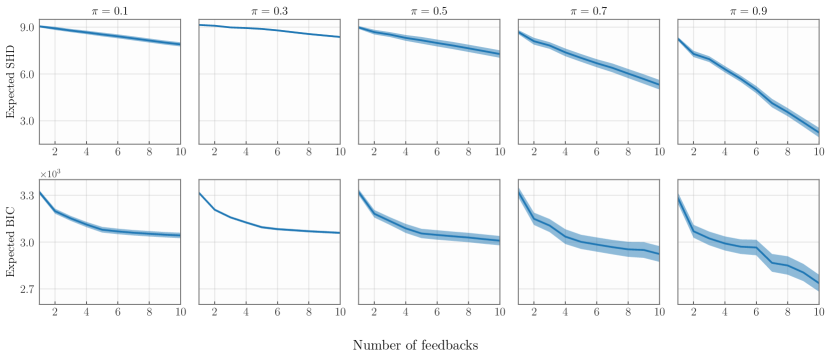
Figure 7: Sensitivity of our active knowledge elicitation framework to the reliability of the expert. Each column represents either the expected SHD (top) or expected BIC (bottom) as a function of the degree of confidence $\pi\in[0,1]$ in the expert as a function of the number of feedbacks. As expected, the improvements entailed by the expert’s feedback become increasingly effective as we increase the expert’s reliability from $0.1$ to $0.9$. Results reflect the outcome of 30 scenarios simulated accordingly to algorithm 1 with a random canonical diagram $\mathcal{G}^{\star}$ with $5$ nodes. We used our active knowledge elicitation scheme to select the query at each iteration.

Training hyperparameters.

For AGFN’s forward flow, we use a Graph Isomorphism Network (GIN, Xu et al. (2019)) with $2$ layers to compute embeddings of dimension $256$. Then, we project these embeddings to a probability distribution using a three-layer MLP having leaky RELUs with a negative slope of $-0.01$ as activation functions. Correspondingly, we use an equally configured three-layer MLP to parametrize AGFN’s backward flow. For training, we use the Adam method for the stochastic optimization problem defined by the minimization of the loss in eq. 7. Moreover, we trained the neural networks for $3000$ epochs for the human-in-the-loop simulations (in which we considered graphs having up to $10$ nodes) and for $500$ epochs for both the assessment of the distributional quality of AGFN and the comparison of AGFN with alternative CD approaches.

Computational settings.

We trained the AGFNs for the experiments in fig. 3 and table 1 and fig. 5 for $500$ epochs in computers equipped with NVIDIA’s V100 GPUs. All the experiments were executed in a cluster of NVIDIA’s V100 GPUs and the algorithms were implemented using the machine learning framework PyTorch. To estimate the PAG corresponding to AGFN’s samples and compute the SHDs reported in table 1, we used the FCI’s implementation of the pcalg package in R considering the d-separations entailed by these samples as a criterion for conditional dependence.

C.3 Human in the loop

Algorithm 1 Simulating humans in the loop

$\{\mathcal{G}_{t}\}_{1\leq t\leq T}\text{ samples from AGFN}$, $\mathcal{G}^{*}=(\mathbf{V},E)$ true ancestral graph, $\pi$ reliability of the expert’s feedback

$p(\omega_{r}=k)\leftarrow\frac{1}{T}\sum_{1\leq t\leq T}1_{\{\omega_{r}=k\text{ in }G_{t}\}}\forall k\in[4],r\in{\mathbf{V}\choose 2}$

$\mathbf{f}\leftarrow\{\}$ $\triangleright$ Set of feedbacks (answers)

$\boldsymbol{r}\leftarrow\{\}$ $\triangleright$ Set of queries (questions)

$K\leftarrow 1$

$\omega_{r}^{*}\leftarrow\text{ relation }r\text{'s feature in }\mathcal{G}^{*}\ \forall r\in{\mathbf{V}\choose 2}$

while $\boldsymbol{r}\neq{\mathbf{V}\choose 2}$ do $\triangleright$ Iteratively request the feedback

     $r_{K}\leftarrow\underset{r\in{\mathbf{V}\choose 2}\setminus\boldsymbol{r}}{\operatorname*{arg\ max}}\ \underset{{f_{r}\sim p(\cdot)}}{\mathbb{E}}[-\mathbf{H}\left(q(\mathcal{G};\mathbf{f}\cup\{f_{r}\}),q(\mathcal{G};\mathbf{f})\right)]$

     $\mathbf{r}\leftarrow\mathbf{r}\cup\{r_{K}\}$

     $f_{K}\sim\text{Cat}\left(\pi\cdot\delta_{\omega_{r_{K}}^{*}}+\left(\frac{1-\pi}{3}\right)\cdot(1-\delta_{\omega_{r_{K}}^{*}})\right)$

     $\mathbf{f}\leftarrow\mathbf{f}\cup\{f_{K}\}$

     $K\leftarrow K+1$

end while

Algorithmic details.

We describe in algorithm 1 our procedure for simulating interactions with an expert. Initially, we estimate the marginal probabilities $p(\omega_{r}=k)$ of a relation $r$ displaying the feature $k\in\{1,2,3,4\}$ under AGFN’s learned distribution. This is our prior distribution. In algorithm 1, we denote $\{1,2,3,4\}$ by $[4]$. Then, we iteratively select the relation that maximizes our acquisition function; the simulated human thus returns a feedback that equals the selected relation’s true feature with probability $\pi$ or is otherwise uniformly distributed among the incorrect alternatives. Importantly, this iterative mechanism can be interrupted at any iteration and the collected feedbacks can be used to compute the importance weights necessary for estimating expectations of functionals under our updated beliefs.

Appendix D Additional experiments

Figure 8: Architectural design of AGFN. Top: The inductively biased parametrization of AGFN’s forward flow — based upon a GNN — enables the substantial reduction of the number of epochs required for training. Bottom: The use of a parametrized backward policy similarly enhances the training efficiency compared to a uniform policy. For both experiments, we considered $\mathcal{L}(\theta)<0.1$ as the early stopping criterion to interrupt AGFN’s training.

Trade-off between diversity and optimality in AGFN.

We may use tempered rewards to increase the frequency of high-scoring samples and thereby reduce the diversity of AGFN’s distribution. More precisely, we choose a temperature $T$ and consider

$$R_{T}(\mathcal{G})=R(\mathcal{G})^{1/T}=\exp\left\{\frac{\mu-U(\mathcal{G})}{T\sigma}\right\}$$ (25)

as the reward upon which the GFlowNet is trained; if $T\rightarrow 0$, the distribution $p_{T}\propto R_{T}$ converges to a point mass in $R(\mathcal{G})$’s mode and, if $T\rightarrow\infty$, $p_{T}$ converges to an uniform distribution. This approach resembles the simulated tempering scheme commonly exploited in Monte Carlo methods Marinari and Parisi (1992) and was previously considered in the context of GFlowNets by Zhang et al. (2023). Figure 6 shows that progressively cold distributions (i.e., with $T\rightarrow 0$) lead to progressively concentrated and decreasingly diverse samples. Notably, the use of cold distributions may be adequate if we are highly confident in our score and are mostly interested in high-scoring samples (e.g., as in Rantanen et al., 2021).

Figure 9: Human-aided AGFN significantly outperforms alternative CD algorithms. Updating AGFN’s distribution according to the feedback of an oracle substantially improves AGFN’s capacity to correctly identify the true ancestral graph; indeed, a single feedback is sufficient to yield results better than (or indistinguishable from) alternative CD algorithms. We select the sampled AG with the highest posterior reward as a point estimate of AGFN and use the same datasets listed in table 2. The plots summarize the results of $30$ HITL simulations using $\pi=0.9$ and an oracle as an expert (see algorithm 1).

Sensitivity analysis for different noise levels.

Figure 7 displays the effect of the feedback of an increasingly reliable expert over the expectations of both the SHD and the BIC. Notably, the usefulness of these feedbacks increases as the feedback noise decreases. This is expected as, for example, a completely unreliable expert consistently rules out only one of four possibilities for the features of each relation; then, there remains a great ambiguity, albeit not as much as there was prior to their feedback, about the true nature of the elicited causal relation. Moreover, this experiment highlights the potential to adjust the reliability parameter $\pi$ to incorporate knowledge into AGFN’s learned distribution regarding the non-existence of a particular relation, rather than its existence. More specifically, assume that the expert is certain that there is no directed edge from the variable $U$ to the variable $V$ in the underlying ancestral graph; for instance, a doctor may be certain that cancer ($U$) is not an ancestor (cause) of smoking ($V$), but may be uncertain about the definite relation between $U$ and $V$ (i.e., smoking may or may not cause cancer). To incorporate such knowledge into our model, one approach is to set a necessarily small reliability parameter $\pi$ (possibly, $\pi=0$) along with the improbable relation $U\rightarrow V$. This feedback will then be modeled as a relation unlikely to exist in the true ancestral graph. We emphasize that our model for the expert’s responses is straightforwardly extensible to accommodate multiple feedbacks about the same causal relation under different reliability levels.

Ablation studies.

Figure 8 shows the increase in the training efficiency due to our architectural designs for parametrizing both the forward and backward flows of AGFN. Noticeably, the use of a two-layer graph isomorphism network (GIN; Xu et al., 2019) with a 256-dimensional embedding for the forward flow entailed a decrease of more than 10x in the number of epochs required for successfully training AGFN; this highlights the effectiveness of an inductively biased architectural design for the parametrization of GFlowNet’s flows. Correlatively, the use of a parametrized backward flow significantly enhances the training efficiency of AGFN and emphasizes the inadequacy of a uniformly distributed backward policy pointed out in a previous work Shen et al. (2023).

Human-aided AGFN versus alternative CD methods.

Figure 9 exposes the significant enhancement of AGFN’s point estimates entailed by our HITL framework for CD. This underlines the usefulness of the elicited knowledge, which is simply incorporated into our model through a re-weighting of the reward function, enabling the identification of the true ancestral graph. In contrast, most alternative CD algorithms cannot be as easily adapted to include various forms of expert knowledge — and such incorporation, when it is possible, usually precedes any inferential process Andrews (2020) or assumes the knowledge is perfect Wang et al. (2022).

References

- Andersen [2013] Holly Andersen. When to expect violations of causal faithfulness and why it matters. Philosophy of Science, 80(5):672–683, 2013.
- Andrews [2020] Bryan Andrews. On the completeness of causal discovery in the presence of latent confounding with tiered background knowledge. In Artificial Intelligence and Statistics (AISTATS), 2020.
- Ashman et al. [2023] Matthew Ashman, Chao Ma, Agrin Hilmkil, Joel Jennings, and Cheng Zhang. Causal reasoning in the presence of latent confounders via neural ADMG learning. In International Conference on Learning Representations (ICLR), 2023. URL https://openreview.net/forum?id=dcN0CaXQhT.
- Bareinboim and Pearl [2016] Elias Bareinboim and Judea Pearl. Causal inference and the data-fusion problem. Proceedings of the National Academy of Sciences, 113(27):7345–7352, 2016. doi: 10.1073/pnas.1510507113. URL https://www.pnas.org/doi/abs/10.1073/pnas.1510507113.
- Bengio et al. [2021a] Emmanuel Bengio, Moksh Jain, Maksym Korablyov, Doina Precup, and Yoshua Bengio. Flow Network based Generative Models for Non-Iterative Diverse Candidate Generation. Advances in Neural Information Processing Systems (NeurIPS), 2021a.
- Bengio et al. [2021b] Yoshua Bengio, Tristan Deleu, Edward J Hu, Salem Lahlou, Mo Tiwari, and Emmanuel Bengio. GFlowNet Foundations. arXiv preprint, 2021b.
- Bernstein et al. [2020] Daniel Bernstein, Basil Saeed, Chandler Squires, and Caroline Uhler. Ordering-based causal structure learning in the presence of latent variables. In Artificial Intelligence and Statistics (AISTATS), 2020.
- Bhattacharya et al. [2021] Rohit Bhattacharya, Tushar Nagarajan, Daniel Malinsky, and Ilya Shpitser. Differentiable causal discovery under unmeasured confounding. In Artificial Intelligence and Statistics (AISTATS), 2021.
- Brouillard et al. [2022] Philippe Brouillard, Perouz Taslakian, Alexandre Lacoste, Sébastien Lachapelle, and Alexandre Drouin. Typing assumptions improve identification in causal discovery. In Causal Learning and Reasoning (CLeaR), 2022.
- Cartwright [1989] Nancy Cartwright. Nature’s Capacities and their Measurement. Clarendon Press, 1989.
- Chen et al. [2016] Eunice Yuh-Jie Chen, Yujia Shen, Arthur Choi, and Adnan Darwiche. Learning bayesian networks with ancestral constraints. In Advances in Neural Information Processing Systems (NeurIPS), 2016.
- Claassen and Heskes [2012] Tom Claassen and Tom Heskes. A bayesian approach to constraint based causal inference. In Uncertainty in Artificial Intelligence (UAI), 2012.
- Claassen et al. [2013] Tom Claassen, Joris M. Mooij, and Tom Heskes. Learning sparse causal models is not np-hard. In Uncertainty in Artificial Intelligence (UAI), 2013.
- Colombo et al. [2012] Diego Colombo, Marloes H Maathuis, Markus Kalisch, and Thomas S Richardson. Learning high-dimensional directed acyclic graphs with latent and selection variables. Annals of Statistics, 2012.
- Colombo et al. [2014] Diego Colombo, Marloes H Maathuis, et al. Order-independent constraint-based causal structure learning. J. Mach. Learn. Res., 15(1):3741–3782, 2014.
- Deleu et al. [2022] Tristan Deleu, António Góis, Chris Chinenye Emezue, Mansi Rankawat, Simon Lacoste-Julien, Stefan Bauer, and Yoshua Bengio. Bayesian structure learning with generative flow networks. In Uncertainty in Artificial Intelligence (UAI), 2022.
- Deleu et al. [2023] Tristan Deleu, Mizu Nishikawa-Toomey, Jithendaraa Subramanian, Nikolay Malkin, Laurent Charlin, and Yoshua Bengio. Joint bayesian inference of graphical structure and parameters with a single generative flow network. arXiv preprint arXiv:2305.19366, 2023.
- Drton and Richardson [2008] Mathias Drton and Thomas S Richardson. Binary models for marginal independence. Journal of the Royal Statistical Society Series B: Statistical Methodology, 2008.
- Drton et al. [2009] Mathias Drton, Michael Eichler, and Thomas S. Richardson. Computing maximum likelihood estimates in recursive linear models with correlated errors. Journal of Machine Learning Research (JMLR), 2009.
- Foygel and Drton [2010] Rina Foygel and Mathias Drton. Extended bayesian information criteria for gaussian graphical models. In Advances in Neural Information Processing (NeurIPS), 2010.
- Geweke [1989] John Geweke. Bayesian inference in econometric models using Monte Carlo integration. Econometrica, 1989.
- Gordon et al. [1993] Neil J Gordon, David J Salmond, and Adrian FM Smith. Novel approach to nonlinear/non-gaussian bayesian state estimation. IEE Proceedings F (Radar and Signal Processing), 1993.
- Hinton [2002] Geoffrey E. Hinton. Training products of experts by minimizing contrastive divergence. Neural Computation, 2002.
- Hyttinen et al. [2014] Antti Hyttinen, Frederick Eberhardt, and Matti Järvisalo. Constraint-based causal discovery: Conflict resolution with answer set programming. In Uncertainty in Artificial Intelligence (UAI), 2014.
- Jabbari et al. [2017] Fattaneh Jabbari, Joseph D. Ramsey, Peter Spirtes, and Gregory F. Cooper. Discovery of causal models that contain latent variables through bayesian scoring of independence constraints. In ECML/PKDD (2), volume 10535 of Lecture Notes in Computer Science, pages 142–157. Springer, 2017.
- Jaber et al. [2022] Amin Jaber, Adele Ribeiro, Jiji Zhang, and Elias Bareinboim. Causal Identification under Markov equivalence: Calculus, Algorithm, and Completeness. In Advances in Neural Information Processing Systems (NeurIPS), 2022.
- Jain et al. [2022] Moksh Jain, Emmanuel Bengio, Alex Hernandez-Garcia, Jarrid Rector-Brooks, Bonaventure F. P. Dossou, Chanakya Ajit Ekbote, Jie Fu, Tianyu Zhang, Michael Kilgour, Dinghuai Zhang, Lena Simine, Payel Das, and Yoshua Bengio. Biological sequence design with GFlowNets. In International Conference on Machine Learning (ICML), 2022.
- Lahlou et al. [2023] Salem Lahlou, Tristan Deleu, Pablo Lemos, Dinghuai Zhang, Alexandra Volokhova, Alex Hernández-Garcıa, Léna Néhale Ezzine, Yoshua Bengio, and Nikolay Malkin. A theory of continuous generative flow networks. In International Conference on Machine Learning, pages 18269–18300. PMLR, 2023.
- Li and Beek [2018] Andrew C. Li and Peter Beek. Bayesian network structure learning with side constraints. In Probabilistic Graphical Models (PGM), 2018.
- Li et al. [2023] Yinchuan Li, Shuang Luo, Yunfeng Shao, and Jianye Hao. Gflownets with human feedback. In Tiny Papers @ (ICLR). OpenReview.net, 2023.
- Lu et al. [2021] Ni Y Lu, Kun Zhang, and Changhe Yuan. Improving causal discovery by optimal bayesian network learning. In AAAI Conference on Artificial Intelligence (AAAI), 2021.
- Ma et al. [2013] Jianzhu Ma, Jian Peng, Sheng Wang, and Jinbo Xu. Estimating the partition function of graphical models using langevin importance sampling. In Proceedings of the Sixteenth International Conference on Artificial Intelligence and Statistics, 2013.
- Magliacane et al. [2016] Sara Magliacane, Tom Claassen, and Joris M Mooij. Ancestral causal inference. Advances in Neural Information Processing Systems (NeurIPS), 2016.
- Marinari and Parisi [1992] E Marinari and G Parisi. Simulated tempering: A new monte carlo scheme. Europhysics Letters (EPL), 19(6):451–458, July 1992.
- Marshall [1954] Andrew W Marshall. The use of multi-stage sampling schemes in Monte Carlo computations. Rand Corporation, 1954.
- Marx et al. [2021] Alexander Marx, Arthur Gretton, and Joris M. Mooij. A weaker faithfulness assumption based on triple interactions. In Uncertainty in Artificial Intelligence (UAI), 2021.
- Meek [1995a] Christopher Meek. Causal inference and causal explanation with background knowledge. In Artificial Intelligence and Statistics (UAI), 1995a.
- Meek [1995b] Christopher Meek. Strong completeness and faithfulness in bayesian networks. In Uncertainty in Artificial Intelligence (UAI), 1995b.
- Newman [2010] M. E. J. Newman. Networks: an introduction. Oxford University Press, 2010.
- Ng et al. [2021] Ignavier Ng, Yujia Zheng, Jiji Zhang, and Kun Zhang. Reliable causal discovery with improved exact search and weaker assumptions. Advances in Neural Information Processing Systems (NeurIPS), 2021.
- Nowzohour et al. [2017] Christopher Nowzohour, Marloes H Maathuis, Robin J Evans, and Peter Bühlmann. Distributional equivalence and structure learning for bow-free acyclic path diagrams. Electronic Journal of Statistics, 2017.
- Ogarrio et al. [2016] Juan Miguel Ogarrio, Peter Spirtes, and Joe Ramsey. A hybrid causal search algorithm for latent variable models. In Probabilistic Graphical Models (PGM), 2016.
- Parviainen and Kaski [2017] Pekka Parviainen and Samuel Kaski. Learning structures of bayesian networks for variable groups. Int. J. Approx. Reason., 88:110–127, 2017.
- Pearl [2000] Judea Pearl. Causality: Models, Reasoning, and Inference. Cambridge University Press, New York, 2000. 2nd edition, 2009.
- Ramsey [2015] Joseph D Ramsey. Scaling up greedy causal search for continuous variables. arXiv preprint, 2015.
- Rantanen et al. [2021] Kari Rantanen, Antti Hyttinen, and Matti Järvisalo. Maximal ancestral graph structure learning via exact search. In Artificial Intelligence and Statistics (UAI), 2021.
- Richardson and Spirtes [2002] Thomas Richardson and Peter Spirtes. Ancestral graph markov models. Annals of Statistics, 2002.
- Ryan et al. [2015] Elizabeth G. Ryan, Christopher C. Drovandi, James M. McGree, and Anthony N. Pettitt. A review of modern computational algorithms for bayesian optimal design. International Statistical Review, 84(1):128–154, 2015.
- Shen et al. [2023] Max W Shen, Emmanuel Bengio, Ehsan Hajiramezanali, Andreas Loukas, Kyunghyun Cho, and Tommaso Biancalani. Towards understanding and improving gflownet training. arXiv preprint arXiv:2305.07170, 2023.
- Silva [2013] Ricardo Silva. A MCMC approach for learning the structure of gaussian acyclic directed mixed graphs. In Statistical Models for Data Analysis, Studies in Classification, Data Analysis, and Knowledge Organization, pages 343–351. Springer, 2013.
- Spirtes and Richardson [1997] Peter Spirtes and Thomas S. Richardson. A polynomial time algorithm for determining dag equivalence in the presence of latent variables and selection bias. In David Madigan and Padhraic Smyth, editors, Proceedings of the Sixth International Workshop on Artificial Intelligence and Statistics, volume R1 of Proceedings of Machine Learning Research, pages 489–500. PMLR, 04–07 Jan 1997. URL https://proceedings.mlr.press/r1/spirtes97b.html. Reissued by PMLR on 30 March 2021.
- Spirtes et al. [2001] Peter Spirtes, Clark N Glymour, and Richard Scheines. Causation, Prediction, and Search. MIT Press, 2nd edition, 2001.
- Triantafillou and Tsamardinos [2016] Sofia Triantafillou and Ioannis Tsamardinos. Score-based vs constraint-based causal learning in the presence of confounders. In Causation: Foundation to Application Workshop (CFA), pages 59–67, 2016.
- Tsirlis et al. [2018] Konstantinos Tsirlis, Vincenzo Lagani, Sofia Triantafillou, and Ioannis Tsamardinos. On scoring Maximal Ancestral Graphs with the Max–Min Hill Climbing algorithm. International Journal of Approximate Reasoning, 102:74–85, 2018. ISSN 0888-613X.
- Uhler et al. [2012] Caroline Uhler, Garvesh Raskutti, Peter Buhlmann, and Bin Yu. Geometry of the faithfulness assumption in causal inference. Annals of Statistics, 2012.
- Wang et al. [2022] Tian-Zuo Wang, Tian Qin, and Zhi-Hua Zhou. Sound and complete causal identification with latent variables given local background knowledge. In Advances in Neural Information Processing Systems (NeurIPS), 2022.
- Xu et al. [2019] Keyulu Xu, Weihua Hu, Jure Leskovec, and Stefanie Jegelka. How powerful are graph neural networks? In International Conference on Learning Representations, (ICLR), 2019.
- Zhalama et al. [2017a] Zhalama, Jiji Zhang, Frederick Eberhardt, and Wolfgang Mayer. Sat-based causal discovery under weaker assumptions. In Artificial Intelligence and Statistics (UAI). AUAI Press, 2017a.
- Zhalama et al. [2017b] Zhalama, Jiji Zhang, and Wolfgang Mayer. Weakening faithfulness: some heuristic causal discovery algorithms. International Journal of Data Science and Analytics, 3(2):93–104, 2017b. ISSN 2364-4168. doi: 10.1007/s41060-016-0033-y. URL https://doi.org/10.1007/s41060-016-0033-y.
- Zhang et al. [2023] David W Zhang, Corrado Rainone, Markus Peschl, and Roberto Bondesan. Robust scheduling with GFlownets. In International Conference on Learning Representations (ICLR), 2023.
- Zhang et al. [2022] Dinghuai Zhang, Nikolay Malkin, Zhen Liu, Alexandra Volokhova, Aaron Courville, and Yoshua Bengio. Generative flow networks for discrete probabilistic modeling. In International Conference on Machine Learning, pages 26412–26428. PMLR, 2022.
- Zhang [2007] Jiji Zhang. A characterization of markov equivalence classes for directed acyclic graphs with latent variables. In Artificial Intelligence and Statistics (UAI), pages 450–457. AUAI Press, 2007.
- Zhang [2008a] Jiji Zhang. Causal reasoning with ancestral graphs. Journal of Machine Learning Research (JMLR), 2008a.
- Zhang [2008b] Jiji Zhang. On the completeness of orientation rules for causal discovery in the presence of latent confounders and selection bias. Artificial Intelligence, 2008b.
- Zhang and Spirtes [2008] Jiji Zhang and Peter Spirtes. Detection of unfaithfulness and robust causal inference. Minds and Machines, 18(2):239–271, Jun 2008. ISSN 1572-8641.
- Zhang and Spirtes [2016] Jiji Zhang and Peter Spirtes. The three faces of faithfulness. Synthese, 193(4):1011–1027, 2016. ISSN 1573-0964. doi: 10.1007/s11229-015-0673-9. URL https://doi.org/10.1007/s11229-015-0673-9.