Robust Approximation Algorithms for Non-monotone $k$-Submodular Maximization under a Knapsack Constraint

Abstract

The problem of non-monotone $k$-submodular maximization under a knapsack constraint (kSMK) over the ground set size $n$ has been raised in many applications in machine learning, such as data summarization, information propagation, etc. However, existing algorithms for the problem are facing questioning of how to overcome the non-monotone case and how to fast return a good solution in case of the big size of data. This paper introduces two deterministic approximation algorithms for the problem that competitively improve the query complexity of existing algorithms. Our first algorithm, LAA, returns an approximation ratio of $1/19$ within $O(nk)$ query complexity. The second one, RLA, improves the approximation ratio to $1/5-\epsilon$ in $O(nk)$ queries, where $\epsilon$ is an input parameter. Our algorithms are the first ones that provide constant approximation ratios within only $O(nk)$ query complexity for the non-monotone objective. They, therefore, need fewer the number of queries than state-of-the-the-art ones by a factor of $\Omega(\log n)$.

Besides the theoretical analysis, we have evaluated our proposed ones with several experiments in some instances: Influence Maximization and Sensor Placement for the problem. The results confirm that our algorithms ensure theoretical quality as the cutting-edge techniques and significantly reduce the number of queries.

I Introduction

$k$-submodular is a generalized version of submodular in polyhedra [1] in which some properties of submodularity have deep theoretical extensions to $k$-submodularity that challenge researchers to study [2, 3, 4], etc. Maximizing a $k$-submodular function subject to some constraints has recently become crucial in combinatorial optimization and machine learning such as influence maximization via social networks [5, 6, 7, 8], sensor placement [5, 6, 7], feature selection [2] and information coverage maximization [7], etc. Given a finite ground set $V$ with $|V|=n$, and an integer number $k$, let $[k]=\{1,2,\ldots,k\}$, and $(k+1)^{V}=\{(V_{1},V_{2},\ldots,V_{k})|V_{i}\subseteq V,\forall i\in[k],V_{i}\cap V_{j}=\emptyset,\forall i\neq j\}$ be a family of $k$ disjoint sets, called the $k$-set. We have the following definition of the $k$-submodular function:

Definition 1 ($k$-submodularity [3]).

A function $f:(k+1)^{V}\mapsto\mathbb{R}_{+}$ is $k$-submodular iff for any ${\textbf{x}}=(X_{1},X_{2},\ldots,X_{k})$ and ${\textbf{y}}=(Y_{1},Y_{2},\ldots,Y_{k})$ $\in(k+1)^{V}$, we have:

$$f({\textbf{x}})+f({\textbf{y}})\geq f({\textbf{x}}\sqcap{\textbf{y}})+f({\textbf{x}}\sqcup{\textbf{y}})$$ (1)

where

$${\textbf{x}}\sqcap{\textbf{y}}=(X_{1}\cap Y_{1},\ldots,X_{k}\cap Y_{k})$$

and

$${\textbf{x}}\sqcup{\textbf{y}}=(Z_{1},\ldots,Z_{k}),\ \mbox{where}\ Z_{i}=X_{i}\cup Y_{i}\setminus(\bigcup_{j\neq i}X_{j}\cup Y_{j})$$

In this paper, we consider the problem of $k$-Submodular Maximization under a Knapsack constraint (kSMK) which is defined as follows:

Definition 2 (The $k$-Submodular Maximization under a Knapsack constraint (kSMK) problem).

Under the knapsack constraint, each element $e$ is assigned a positive cost $c(e)$. Given a limited budget $B>0$, the problem kSMK asks to find a $k$-set ${\textbf{x}}=(X_{1},X_{2},\ldots,X_{k})$ with total cost $c({\textbf{x}})=\sum_{e\in X_{i},i\in[k]}c(e)\leq B$ so that $f({\textbf{x}})$ is maximized.

The problem kSMK is a general model applied to a lot of essential instances such as $k$-topic influence maximization, $k$-type sensor placement, $k$-topic information coverage maximization [9, 10, 11], etc., with the knapsacks that encode users’ constraints including budget, time or size. For example, $k$-topic influence maximization under knapsack constraint (kSMK) [3, 10, 6], the problem asks for maximizing the expected number of users, who are influenced by at least one of $k$ distinct topics with a limited budget $B>0$. The mathematical nature is $k$-submodular maximization under a diffusion model, which Kempe et al.[12] first proposed with a single type of influence.

The challenge when providing a solution for kSMK is it has many candidate approximate solutions with different sizes. We have to select the best nearly optimal one within polynomial time. Therefore, beyond obtaining a nearly optimal solution to kSMK in the aforementioned applications, designing such a solution must also minimize the query complexity, especially for big data, since the tremendous amount of input data makes the search space for a solution crazily soar. Unfortunately, $k$-submodularity requires an algorithm to evaluate the objective function whenever observing an incoming element. Therefore, it is necessary to design efficient algorithms in reasonable computational time. We refer to the query complexity as a measure of computational time since it dominates the time running of an algorithm. Previous works [13, 14, 11] proposed efficient algorithms for kSMK in which even some algorithms can provide solutions in linear query complexity of $O(kn)$. However, these works are just available for the monotone case. Meanwhile, some works [15, 16, 17] showed that the $k$-submodular objective function might be non-monotone in practical applications. Therefore, solving the $\mathsf{\mbox{non-monotone }kSMK}$ problem within linear query complexity is critical.

Overall, this paper aims to tackle both challenges above for non-monotone $k$-submodular maximization and constrained by a knapsack.

I-A Our contribution

In this work, we design novel approximate algorithms that respond to some requirements about providing considerable solution quality and reducing query complexity. In particular, our work is the first one that provides a constant approximation ratio within only $O(kn)$ query complexity for $\mathsf{\mbox{non-monotone }kSMK}$. The main version, RLA returns an approximation ratio of $1/5-\epsilon$ which is equivalent to the state-of-the-art one proposed in [18]. In general, our contributions are as per the following:

• We first propose the LAA algorithm (Algorithm 1), a $1/19$-approximation one that scans a single pass over the ground set within $O(kn)$ query complexity. It’s the first simple but vital algorithm of our work since it limits the range of the optimal value. Besides, it provides a data division strategy to reduce query complexity to $O(nk)$.

• We next propose RLA algorithm (Algorithm 2) that achieves an approximation ratio $1/5-\epsilon$, and requires $O(kn/\epsilon)$ query complexity where $\epsilon>0$ is an accuracy parameter. Specifically, to the best of our knowledge, our algorithm is also equivalent to the current best approximation ratio of a deterministic algorithm for the studied problem in [18].

• To illustrate the theoretical contributions, we conduct several comprehensive experiments in two applications of kSMK including $k$-topic Influence Maximization and $k$-type Sensor Placement. Experimental results have shown that our algorithms save queries more than state-of-the-art (mentioned in Table I) and return comparable results in terms of performance.

Table I compares our algorithms with some state-of-the-art algorithms for $\mathsf{\mbox{non-monotone }kSMK}$ on three aspects, including approximation ratio, query complexity, and deterministic or not. These fields indicate that our algorithms have both a low number of queries and valuable deterministic approximation ratios that are equivalent to or even better than the others.

Reference	Approximation ratio	Query complexity	Is deterministic?
LAA (Alg. 1, this paper)	$1/19$	$O(kn)$	Yes
RLA (Alg. 2, this paper)	$1/5-\epsilon$	$O(kn/\epsilon)$	Yes
Deterministic Streaming[18]	$1/5-\epsilon$	$O(kn\log(n)/\epsilon)$	Yes
Random Streaming[18]	$k/(5k-2)-\epsilon$	$O(kn\log(n)/\epsilon)$	No

TABLE I: Algorithm comparison for $\mathsf{\mbox{non-monotone }kSMK}$; Note that Desterministic Streaming and Random Streaming in [18] is the special case when $\beta=1$.

Organization The rest of the paper is organized as follows: We provide a literature review and discussions in Section II. The notations and properties of $k$-submodular functions are presented in Section III. Section IV presents our algorithms and theoretical analysis. The extensive experiments are shown in Section V. Finally, we conclude this work in Section VI.

II Related work

In this section, we review related works and provide some discussion on existing algorithms.

Studying $k$-submodular functions appears when considering the submodularity in polyhedra. Lovász [1] found that it was a similar but deeper theory than submodularity when working with intersection matroids. After that, more works have focused on the issue of $k$-submodularity with general $k\geq 2$. First, people studied maximizing unconstrained $k$-submodular [3, 19, 20]. Due to the practical values when solving the problem with constraints, some authors focused on $k$-submodular maximization under some kinds of constraints [5, 21, 22], etc. Authors focused on the monotone case such as Oshaka et al. [5] studied monotone $k$-submodular maximization with two kinds of size constraint: overall size constraint and singular size constraint, authors in [10] proposed a multi-objective evolutionary method to provide an approximation ratio of $1/2$ for the monotone $k$-submodular maximization problem with the overall size constraint. However, this algorithm took a high query complexity of $O(kn\log^{2}B)$ in expectation. Authors [23] further proposed an online algorithm with the same approximation ratio of $1/2$ but runs in polynomial time with regret bound. However, these contributions just work for the monotone case and for size constraints; hence, it’s hard to adapt to $\mathsf{\mbox{non-monotone }kSMK}$. Moreover, these algorithms required exponential running time [5] or high query complexity [10].

Recently, Nguyen et al.[8] first applied streaming to solve the problem of $k$-submodular maximization with overall size constraint. Streaming fashion is an active approach when it requires only a small amount of memory to store data and scans one or a few times over the ground set $V$. They devised two streaming algorithms within $O(nk\log(k))$ query complexity. Their first one is deterministic and returns an approximation ratio of $1/3-\epsilon$, while the second one is randomized and returns an approximation ratio of $k/(3k-1)-\epsilon$. Later on, Ene and Nguyen [24] developed a single-pass streaming algorithm based on integer programming formulation for $k$-submodular maximization with singular size constraint with an approximation ratio of $0.5/(1+B(2^{1/B}-1))$ within $O(nk)$ queries, where $B=\min_{i\in[k]}B_{i}$.

Unlike cardinality or matroid, which just enumerates elements, the knapsack requires maximizing $f(\cdot)$ subject to a given budget that the total cost of a solution can not exceed. Hence, there can be multiple maximal cost solutions that are not the same size. The authors [14] proposed a multi-linear extension method with an approximation ratio of $1/2-2\epsilon$ in expectation for the kSMK. This work provides the best approximation ratio in expectation. However, this algorithm is impractical due to the high query complexity of a continuous extension [25].

Besides, Wang et al. [13] proposed a $(1/2-1/(2e))$-approximation algorithm for the kSMK that inspired from the Greedy algorithm in [26]. This algorithm, however, requires an expensive query complexity of $O(n^{4}k^{3})$, and therefore it is difficult to apply to medium-sized instances even though one can compute the objective function $f$ in $O(1)$ time. The authors [14] proposed a multi-linear extension that provided the approximation ratio of $1/2-2\epsilon$ in expectation for the kSMK. This work provides the best approximation ratio in expectation, however, it is impractical because of the high query complexity of a continuous extension [25]. Authors [11] first proposed a $(1/4-\epsilon)$-desterministic approximation algorithm within $O(kn/\epsilon)$. Nonetheless, the aforementioned works are not available for the non-monotone case.

To state the non-monotone $k$-submodularity, Pham et al. [18] recently have proposed two single-pass streaming algorithms for the $k$-submodular maximization under the budget constraint, a general of knapsack constraint within $O(nk\log(n)/\epsilon)$ queries. These algorithms returned the ratios of $1/5-\epsilon$ and $k/(5k-2)-\epsilon$ (in expectation) for the non-monotone case. Our best algorithm version, RLA, gives an equivalent performance of them ($1/5-\epsilon)$ approximation ratio) yet reduces the query complexity to $O(kn/\epsilon)$.

On the whole, the characteristic of our algorithms is deterministic, linear query complexity, and available for non-monotonicity.

III Preliminaries

Notations. Given a ground set $V=\{e_{1},e_{2},\ldots,e_{n}\}$ and an integer $k$, we define $[k]=\{1,2,\ldots,k\}$ and let $(k+1)^{V}=\{(V_{1},V_{2},\ldots,V_{n})|V_{i}\subseteq V\ \forall i\in[k],V_{i}\cap V_{j}=\emptyset\ \forall i\neq j\}$ be a family of $k$ disjoint subsets of $V$, called $k$-set.

For ${\textbf{x}}=(X_{1},X_{2},\ldots,X_{k})\in(k+1)^{V}$, we define $supp_{i}({\textbf{x}})=X_{i}$, $supp({\textbf{x}})=\cup_{i\in[k]}X_{i}$, $X_{i}$ as $i$-th set of x and an empty $k$-set ${\textbf{0}}=(\emptyset,\ldots,\emptyset)$. We set if $e\in X_{i}$ then ${\textbf{x}}(e)=i$ and $i$ is called the position of $e$ in x, otherwise ${\textbf{x}}(e)=0$. Adding an element $e\notin supp({\textbf{x}})$ into $X_{i}$ can be represented by ${\textbf{x}}\sqcup(e,i)$. We also write ${\textbf{x}}=\{(e_{1},i_{1}),(e_{2},i_{2}),\ldots,(e_{t},i_{t})\}$ for $e_{j}\in supp({\textbf{x}}),i_{j}={\textbf{x}}(e_{j}),\forall 1\leq j\leq t$. When $X_{i}=\{e\}$, and $X_{j}=\emptyset,\forall j\neq i$, x is denoted by $(e,i)$.

For ${\textbf{x}}=(X_{1},X_{2},\ldots,X_{k}),{\textbf{y}}=(Y_{1},Y_{2},\ldots,Y_{k})\in(k+1)^{V}$, we denote by ${\textbf{x}}\sqsubseteq{\textbf{y}}$ iff $X_{i}\subseteq Y_{i}$ $\forall i\in[k]$.

The objective function. The function $f:(k+1)^{V}\mapsto\mathbb{R}_{+}$ is $k$-submodular iff for any ${\textbf{x}}=(X_{1},X_{2},\ldots,X_{k})$ and ${\textbf{y}}=(Y_{1},Y_{2},\ldots,Y_{k})$ $\in(k+1)^{V}$, we have:

$$f({\textbf{x}})+f({\textbf{y}})\geq f({\textbf{x}}\sqcap{\textbf{y}})+f({\textbf{x}}\sqcup{\textbf{y}})$$ (2)

where

$${\textbf{x}}\sqcap{\textbf{y}}=(X_{1}\cap Y_{1},\ldots,X_{k}\cap Y_{k})$$

and

$${\textbf{x}}\sqcup{\textbf{y}}=(Z_{1},\ldots,Z_{k}),\ \mbox{where}\ Z_{i}=X_{i}\cup Y_{i}\setminus(\bigcup_{j\neq i}X_{j}\cup Y_{j})$$

For any ${\textbf{x}}\in(k+1)^{V}$, $e\notin supp({\textbf{x}})$ and $i\in[k]$, we have the marginal gain when adding an element $e$ to the $i$-set $X_{i}$ of x is:

$$\Delta_{(e,i)}f({\textbf{x}})= f(X_{1},\ldots,X_{i-1},X_{i}\cup\{e\},X_{i+1},\ldots,X_{k})$$

$$-f(X_{1},\ldots,X_{k})$$

In this work, we consider $f$ to be non-monotone, i.e., the marginal gain when adding a tuple $(e,i)$ to set x, $\Delta_{(e,i)}f({\textbf{x}})$, may be negative. we also assume that $f$ is normalized, i.e, $f({\textbf{0}})=0$, and there exists an oracle query, which when queried with the $k$-set x returns the value $f({\textbf{x}})$. We also recap some properties of the $k$-submodular function that will be used for designing our algorithms.

From [3], a $k$-submodular function $f:(k+1)^{V}\mapsto\mathbb{R}_{+}$ is $k$-submodular iff it is pairwise monotone and orthant submodular. The $k$-submodularity of $f$ implies the orthant submodularity, i.e.,

$$\Delta_{(e,i)}f({\textbf{x}})\geq\Delta_{(e,i)}f({\textbf{y}})$$ (3)

for any ${\textbf{x}},{\textbf{y}}\in(k+1)^{V}$ with ${\textbf{x}}\sqsubseteq{\textbf{y}}$, $e\notin supp({\textbf{y}})$ and $i\in[k]$, and the pairwise monotonicity, i.e.,

$$\Delta_{(e,i)}f({\textbf{x}})+\Delta_{(e,j)}f({\textbf{x}})\geq 0$$ (4)

for any ${\textbf{x}}\in(k+1)^{V}$ with $e\notin supp({\textbf{x}})$ and $i,j\in[k]$ with $i\neq j$.

The problem definition. Assuming that each element $e$ is assigned a positive cost $c(e)$ and the total cost of a $k$-set x $c({\textbf{x}})=\sum_{e\in supp({\textbf{x}})}c(e)$. Given a limited budget $B>0$, we assume that every item $e\in V$ satisfies $c(e)\leq B$; otherwise, we can simply discard it. The $k$-Submodular Maximization under Knapsack constraint (kSMK) problem is to determine:

$$\arg\max_{{\textbf{x}}\in(k+1)^{V}:c({\textbf{x}})\leq B}f({\textbf{x}}).$$ (5)

It means the problem finds the solution x so that the total cost of x is less than or equal to $B$ so that $f({\textbf{x}})$ is maximized. In this work, we only consider $k\geq 2$ because if $k=1$, the $k$-submodular function becomes the submodular function.

IV The algorithms

In this section, we introduce two deterministic algorithms for kSMK. The first algorithm, named Linear Approximation Algorithm (LAA), has an approximation ratio of $1/19$ and takes $O(nk)$ query complexity. Although this approximation ratio is small, it is the first one that gives a constant approximation ratio within only $O(kn)$ queries for the non-monotone case. The approximation ratio is improved by our second algorithm, named Robust Linear Approximation (RLA), from $1/19$ to $1/5-\epsilon$ by recalling the first algorithm’s solution to provide a suitable range for bounding the optimal value ${\mathsf{opt}}$. Additionally, it scans the ground set $O(1/\epsilon)$ times and integrates the decreasing threshold strategy to get the near-optimal solution.

IV-A Linear Approximation Algorithm

Our LAA algorithm adapts the idea of the recent work [11] that (1) divides the ground set $V$ into two subsets: The elements with costs greater than $B/2$ are included in the first subset, while the remaining is included in the second, and (2) near-optimal solutions are sought and combined for the two aforementioned subsets.

Input: $V$, $f$, $k$, $B>0$.

Output: A solution s

1 ${\textbf{x}}\leftarrow{\textbf{0}}$; $(e_{m},i_{m})\leftarrow(\emptyset,1)$; ${\textbf{x}}^{\prime}\leftarrow{\textbf{0}}$;

2 foreach $e\in V$ do

3      $i_{e}\leftarrow\arg\max_{i\in[k]}f((e,i))$

4      $(e_{m},i_{m})\leftarrow\arg\max_{(e^{\prime},i^{\prime})\in\{(e_{m},i_{m}),(e,i_{e})\}}f((e^{\prime},i^{\prime}))$

5      if $c(e)\leq B/2$ then

6           if $\Delta_{(e,i_{e})}f({\textbf{x}})\geq c(e)f({\textbf{x}})/B$ then

7                ${\textbf{x}}\leftarrow{\textbf{x}}\sqcup(e,i_{e})$

8                end if

9               

10                end if

11               

12                end foreach

13               ${\textbf{x}}^{\prime}\leftarrow\arg\max_{{\textbf{x}}_{j}:j\leq t_{x},c({\textbf{x}}_{j})\leq B}c({\textbf{x}}_{j})$, where $t_{x}=|supp({\textbf{x}})|$ and ${\textbf{x}}_{j}=\{(e_{t_{x}-j+1},i_{t_{x}-j+1}),(e_{t_{x}-j+2},i_{t_{x}-j+2}),\ldots,(e_{t_{x}},i_{t_{x}})\}$ is the last $j$ tuples added into x.

14                ${\textbf{s}}\leftarrow\arg\max_{{\textbf{s}}\in\{(e_{m},i_{m}),{\textbf{x}}^{\prime}\}}f({\textbf{s}})$

return ${\textbf{s}}_{final}$

Algorithm 1 An Linear Approximation Algorithm (LAA)

In particular, the algorithm first receives an instance $(V,f,k,B)$ of kSMK and initiates a candidate solution x as an empty set and a tuple $(e_{m},i_{m})$ as $(\emptyset,1)$. The target of the tuple $(e_{m},i_{m})$ is to update the optimal solution found in the first subset, while the candidate solution x is to locate what solution is close to the optimal in the second. For each incoming element $e$, the algorithm finds “the best” position $i_{e}$ in terms of the set $i$ in $k$ sets that returns the highest value $f((e,i_{e}))$. If its cost is greater than $B/2$, the role of $(e_{m},i_{m})$ is the best solution on the current first subset (line 5). Otherwise, the algorithm adds the tuple $(e,i_{e})$ into x if the condition $\Delta_{(e,i_{e})}f({\textbf{x}})\geq c(e)f({\textbf{x}})/B$ is maintained. After the main loop completes, the algorithm selects a $k$-set ${\textbf{x}}^{\prime}$ as the set of last $j$ tuples adding into x with the maximum total cost nearest to $B$ (line 11). Finally, the algorithm returns the final solution s as the best one between $(e_{m},i_{m})$ and ${\textbf{x}}^{\prime}$. The details of the algorithm are fully presented in Algorithm 1.

To deal with the non-monotonicity of the objective function, we have to use non-trivial analyzes to give an approximation. Differing from the monotone case in [11], we use the property of pairwise monotonicity as a critical component in our theoretical analysis. In the following, we analyze the theoretical guarantee of the Algorithm 1. We first define the notations as follows:

• $V_{1}=\{e\in V:c(e)>B/2\},V_{2}=\{e\in V:c(e)\leq B/2\}$.

• o is an optimal solution of the problem over $V$ and the optimal value ${\mathsf{opt}}=f({\textbf{o}})$.

• ${\textbf{o}}^{\prime}_{1}=\{(e,{\textbf{o}}(e)):e\in V_{1}\},{\textbf{o}}^{\prime}_{2}=\{(e,{\textbf{o}}(e)):e\in V_{2}\}$.

• ${\textbf{o}}_{1}$ is an optimal solution of the problem over $V_{1}$.

• ${\textbf{o}}_{2}$ is an optimal solution of the problem over $V_{2}$.

• $(e_{j},i_{j})$ as the $j$-th element added of the main loop of the Algorithm 1.

• ${\textbf{x}}=\{(e_{1},i_{1}),\ldots,(e_{t},i_{t})\}$ the $k$-set x after ending the main loop, $t=|supp({\textbf{x}}|$.

• ${\textbf{x}}^{j}=\{(e_{1},i_{1}),\ldots,(e_{j},i_{j})\}$: the $k$-set x (in the main loop) after adding $j$ elements $1\leq j\leq t$, ${\textbf{x}}^{0}={\textbf{0}}$, ${\textbf{x}}^{t}={\textbf{x}}$.

• ${\textbf{x}}_{j}=\{(e_{t-j+1},i_{t-j+1}),(e_{t-j+2},i_{t-j+2}),\ldots,(e_{t},i_{t})\}$ is the set of last $j$ elements added into x.

• ${\textbf{o}}_{2}^{j}=({\textbf{o}}_{2}\sqcup{\textbf{x}}^{j})\sqcup{\textbf{x}}^{j}$.

• ${\textbf{o}}_{2}^{j-1/2}=({\textbf{o}}_{2}\sqcup{\textbf{x}}^{j})\sqcup{\textbf{x}}^{j-1}$.

• ${\textbf{x}}^{j-1/2}$: If $e_{j}\in supp({\textbf{o}}_{2})$, then ${\textbf{x}}^{j-1/2}={\textbf{x}}^{j-1}\sqcup(e_{j},{\textbf{o}}_{2}(e_{j}))$. If $e_{j}\notin supp({\textbf{o}}_{2})$, ${\textbf{x}}^{j-1/2}={\textbf{x}}^{j-1}$.

• ${\textbf{u}}^{t}=\{(u_{1},i_{1}),(u_{2},i_{2}),\ldots,(u_{r},i_{r})\}$ is a set of elements that are in ${\textbf{o}}_{2}^{t}$ but not in ${\textbf{x}}^{t}$, $r=|supp({\textbf{u}}^{t})|$.

• ${\textbf{u}}^{t}_{l}={\textbf{x}}^{t}\sqcup\{(u_{1},i_{1}),(u_{2},i_{2}),\ldots,(u_{l},i_{l})\},1\leq l\leq r$ and ${\textbf{u}}^{t}_{0}={\textbf{x}}^{t}$.

Supposing that ${\textbf{x}}^{\prime}$ gets $T$ last tuples in x, i.e., ${\textbf{x}}^{\prime}={\textbf{x}}_{T}$. Denote $Q=t-T$, we have ${\textbf{x}}={\textbf{x}}^{Q}\sqcup{\textbf{x}}^{\prime}$. The following Lemmas connect the candidate solution x with ${\textbf{o}}_{2}$.

Lemma 1.

$f({\textbf{o}}_{2})-f({\textbf{o}}_{2}^{j})\leq 2f({\textbf{x}}^{j})$ for all $0\leq j\leq t$.

Proof.

See the Appendix, section VI-A ∎

Lemma 2.

$f({\textbf{x}}^{\prime})\geq f({\textbf{x}}^{t})/3$.

Proof.

See the Appendix, section VI-A ∎

Lemma 3.

$f({\textbf{o}}_{2}^{t})\leq 4f({\textbf{x}}^{t})$.

Proof.

See the Appendix, section VI-A ∎

From these above lemmas, we imply the following lemma:

Lemma 4.

$f({\textbf{x}}^{\prime})\geq f({\textbf{o}}_{2})/18$.

Proof.

See the Appendix, section VI-A ∎

Theorem 1.

Algorithm 1 is a single-pass streaming algorithm that returns an approximation ratio of $1/19$ and takes $nk$ queries.

Proof.

See the Appendix, section VI-A ∎

IV-B A Robust Linear Approximation Algorithm

We next introduce the RLA algorithm, which improves the approximation ratio to $1/5-\epsilon$ and takes $O(kn/\epsilon)$ query complexity. RLA keeps the key idea of LAA by reusing the LAA’s solution to bounding the ${\mathsf{opt}}$’s range and adapts a greedy threshold to improve the approximation ratio by conducting $O(1/\epsilon)$ times scanning over the ground set. The details of the algorithm are fully presented in Algorithm 2.

Input: $V$, $f$, $k$, $B>0$, $\epsilon>0$.

Output: A solution s

1 ${\textbf{s}}_{b}\leftarrow$ result of Algorithm 1; $\Gamma\leftarrow f({\textbf{s}}_{b})$

2 $A\leftarrow\{(1+\epsilon)^{i}:i\in\mathbb{N},\Gamma\leq(1+\epsilon)^{i}\leq 19\Gamma\}$

3 for $e\in V$ do

4      foreach $v\in A$ do

5           $i_{v}\leftarrow\arg\max_{i\in[k]}\Delta_{(e,i)}f({\textbf{s}}_{v})$

6           $\tau_{v}=2v/(5B)$

7           if $c({\textbf{s}}_{v})+c(e)\leq B\ \mbox{{and}}\ \Delta_{(e,i_{v})}f({\textbf{s}}_{v})/c(e))\geq\tau_{v}$ then

8                ${\textbf{s}}_{v}\leftarrow{\textbf{s}}_{v}\sqcup(e,i_{v})$

9               

10                end if

11               

12                end foreach

13               

14                end for

${\textbf{s}}_{final}\leftarrow\arg\max_{{\textbf{s}}^{\prime}\in\{{\textbf{s}}_{max},{\textbf{s}}_{1},{\textbf{s}}_{2},\ldots,{\textbf{s}}_{|S|}\}}f({\textbf{s}}^{\prime})$ return ${\textbf{s}}_{final}$

Algorithm 2 Robust Linear Approximation (RLA) Algorithm

Specifically, RLA takes an instance $(V,f,k,B)$ of kSMK and an accuracy parameter $\epsilon>0$ as inputs. RLA first calls LAA as a subroutine and uses LAA’s solution, ${\textbf{s}}_{b}$, to obtain a bound range of the optimal solution (line 1). From Theorem 1, we have $\Gamma\leq{\mathsf{opt}}\leq 19\Gamma$.

The major part of the algorithm consists of two loops: the outer to scan each element $e$ in the ground set $V$ and the inner to consider each candidate solution ${\textbf{s}}_{v}$ for each $v$ filtered out from the set $A$. On the basis of Theorem 1, we construct the set $A$ to bound the number of candidate solutions ${\textbf{s}}_{v}$. We define $(e,i_{v})$ as the tuple that gives the largest marginal gain when added into ${\textbf{s}}_{v}$. When an element $e$ arrives, the algorithm handles these works: (1) choose the position $i_{v}$ with maximal marginal gain with respect to ${\textbf{s}}_{v}$ and $e$ (line (2)); (2) use threshold $\tau_{v}=2v/(5B)$ to add the element $e$ into ${\textbf{s}}_{v}$ if it has the high density gain that is defined as the ratio of the marginal gain of that element over its cost without violating the budget constraint (line (2)).

We still keep the notations o as an optimal solution of the problem over $V$ and the optimal value ${\mathsf{opt}}=f({\textbf{o}})$. We add some notations regarding to Algorithm 2 as follows:

• ${\textbf{s}}_{v}=\{(e_{1},i_{1}),(e_{2},i_{2}),\ldots,(e_{q},i_{q})\}$ is the candidate solution with respect to some elements $v\in A$ after ending the outer loop.

• ${\textbf{s}}^{j}_{v}=\{(e_{1},i_{1}),(e_{2},i_{2}),\ldots,(e_{j},i_{j})\},1\leq j\leq q$ and ${\textbf{s}}^{0}_{v}={\textbf{0}}$.

• ${\textbf{s}}_{v}^{<e}$ as ${\textbf{s}}_{v}$ right before $e$ is processed.

• ${\textbf{u}}=\{(u_{1},i_{1}),(u_{2},i_{2}),\ldots,(u_{r},i_{r})\}$ as a set of elements belongs to o yet doesn’t belong to ${\textbf{s}}_{v}$, $r=|supp({\textbf{u}})|$.

• ${\textbf{u}}_{l}={\textbf{s}}_{v}\sqcup\{(u_{1},i_{1}),(u_{2},i_{2}),\ldots,(u_{l},i_{l})\},\forall 1\leq l\leq r$ and ${\textbf{u}}_{0}={\textbf{s}}_{v}$.

• ${\textbf{o}}^{j}=({\textbf{o}}\sqcup{\textbf{s}}^{j})\sqcup{\textbf{s}}^{j}$.

• ${\textbf{o}}^{j-1/2}=({\textbf{o}}\sqcup{\textbf{s}}^{j})\sqcup{\textbf{s}}^{j-1}$.

• ${\textbf{s}}^{j-1/2}$: If $e_{j}\in supp({\textbf{o}})$, then ${\textbf{s}}^{j-1/2}={\textbf{s}}^{j-1}\sqcup(e_{j},{\textbf{o}}(e_{j}))$. If $e_{j}\notin supp({\textbf{o}})$, ${\textbf{s}}^{j-1/2}={\textbf{s}}^{j-1}$.

Lemma 5.

For any $v\in A$, if there is no element $o\in supp({\textbf{o}})\setminus supp({\textbf{s}}_{v})$ so that $\Delta_{(o,{\textbf{o}}(o))}f({\textbf{s}}^{<o}_{v})\geq\tau_{v}$ and $c({\textbf{s}}_{v}^{<o})+c(o)>B$, we have: $f({\textbf{o}})\leq 3f({\textbf{s}}_{v})+c({\textbf{o}})\tau_{v}$.

Proof.

See the Appendix, section VI-A ∎

Theorem 2.

For $0<\epsilon<1/5$, the Algorithm 2 returns an approximation ratio of $1/5-\epsilon$, within $O(nk/\epsilon)$ queries.

Proof.

See the Appendix, section VI-A ∎

V Experiments

In this section, we compare the performance between our algorithms and state-of-the-art algorithms for the kSMK problem listed below:

• Deterministic Streaming (DS): A streaming algorithm in [18] which returns an approximation ratio of $1/5-\epsilon$, requires 1-pass and $O(kn\log(n)/\epsilon)$ queries.

• Random Streaming (RS): Another streaming algorithm in [18] which returns an approximation ratio of $k/(5k-2)-\epsilon$ in expectation, requires one pass and $O(kn\log(n)/\epsilon)$ queries.

Although Greedy proposed by [13] gives the best approximation ratio yet it is only available for the monotone case. Besides, in [11], authors also showed that the running time of Greedy was so long that they had to limit the time to cut off the experiment. Therefore, in the experiment, we eliminated the Greedy. Also, we conduct experiments on specific applications, which are $k$-topic Influence Maximization under knapsack constraint (kIMK) and $k$-type Sensor Placement under Knapsack constraint (kSPK) on three important measurements: the oracle value of the objective function, the number of queries, and running time. We further show the trade-off between the solution quality and the number of queries of algorithms with various settings of budget $B$.

We also use the dataset as mentioned in [8] to illustrate the performance of compared algorithms (Table II). To demonstrate the performance of algorithms via the above three measurements, we show some figures numbered and captioned, in which the terms Fig, K, and M stand for Figure, thousands, and millions, respectively.

All the implementations are on a Linux machine with configurations of $2\times$ Intel Xeon Silver $4216$ Processor @$2.10$GHz and $16$ threads x$256$GB DIMM ECC DDR4 @$2666$MHz.

TABLE II: The dataset

Database	#Nodes	#Edges	Types	Instances
Facebook [27]	4039	88234	directed	kIMK
Intel Lab sensors[28]	56	-	-	kSPK

V-A $k$-topic Influence Maximization under Knapsack constraint (kIMK)

The information diffusion model, called Linear Threshold (LT) model [12, 8] was briefed, and the $k$-topic Influence Maximization under Knapsack constraint (kIMK) problem using this model was defined as follows:

LT model

A social network is modeled by a directed graph $G=(V,E)$, where $V,E$ represent sets of users and links, respectively. Each edge $(u,v)\in E$ is assigned weights $\{w^{i}(u,v)\}_{i\in[k]}$, where each $w^{i}(u,v)$ represents how powerful $u$ influences to $v$ on the $i$-th topic. Each node $u\in V$ has a influence threshold with topic $i$, denoted by $\theta^{i}(u)$, which is chosen uniformly at random in $[0,1]$. Given a seed set ${\textbf{s}}=(S_{1},S_{2},\ldots,S_{k})\in(k+1)^{V}$, the information propagation for topic $i$ happens in discrete steps $t=0,1,\ldots$ as follows. At step $t=0$, all nodes in $S_{i}$ become active by topic $i$. At step $t\geq 1$, a node $u$ becomes active if $\sum_{\mbox{actived}v}w^{i}(v,u)\geq\theta^{i}(u)$.

The information diffusion process on topic $i$ ends at step $t$ if there is no new active node and the diffusion process of a topic is independent of the others. Denote by $\sigma({\textbf{s}})$ the number of nodes that become active in at least one of $k$ topics after the diffusion process of a seed $k$-set s, i.e.,

$$\sigma({\textbf{s}})=\mathbb{E}[|\cup_{i\in[k]}\sigma_{i}(S_{i})|]$$ (6)

where $\sigma_{i}(S_{i})$ is a random variable representing the set of active users for topic $i$ with the seed $S_{i}$.

The kIMK problem

The problem is formally defined as follows:

Definition 3 (kIMK problem).

Assuming that each user $e$ has a cost $c(e)>0$ for every $i$-th topic, which illustrates how difficult it is to initially influence the appropriate individual about that topic. Given a budget $B>0$, the problem asks to find a seed set s with $c({\textbf{s}})=\sum_{e\in S_{i},i\in k}c(e)\leq B$ so that $\sigma({\textbf{s}})$ maximal.

V-B $k$-type Sensor Placement under Knapsack constraint

We further study the performance of algorithms for $k$-type Sensor Placement under Knapsack constraint (kSPK) problem which is formally defined as follows:

Definition 4 (kSPK problem).

Given $k$ kinds of sensors for different measures and a set $V$ of $n$ locations, each of which is assigned with only one sensor. Assuming that each sensor $e$ has a cost $c(e)>0$ for every $i$-th type. Given a budget $B>0$, the problem aims to locate these sensors to maximize the information gained with the total cost at most $B$.

Denote by $R_{e}^{i}$ a random variable representing the observation collected from a $i$-type sensor and the information gained of a $k$-set s is

$$f({\textbf{s}})=H(\cup_{e\in supp({\textbf{s}})}\{R_{e}^{i}\})$$ (7)

where $H$ is an entropy function.

V-C Results and discussion

V-C1 Experiment settings

For kIMK. We use the dataset Facebook and set up the model as the recent work [8].

Since the computation of $\sigma(\cdot)$ is #P-hard [29], we adapt the sampling method in [8, 30] to give an estimation $\hat{\sigma}(\cdot)$ with a $(\lambda,\delta)$-approximation that is:

$$\Pr[(1+\lambda)\sigma({\textbf{s}})\geq\hat{\sigma}({\textbf{s}})\geq(1-\lambda)\sigma({\textbf{s}})]\geq 1-\delta$$ (8)

It’s said that $\hat{\sigma}(\cdot)$ is $\epsilon$-estimation of $\sigma(\cdot)$ with probability at least $\lambda$. As [8, 18], in the experiment, we set parameters $\lambda=0.8,\delta=0.2$, $k=3$ and $\epsilon=0.1$ to show a trade-off between solution quality and quantities of queries.

We set $B$ in $\{0.5K,1K,1.5K,2K\}$ to illustrate the expense to influence $k$ topics via social networks is not a small number and set the cost of each element from 1 to 10 according to the Normalized Linear model [18].

For kSPK. We use the dataset Intel Lab [28] to illustrate the kSPK problem. The data were preprocessed to remove missing fields. Moreover, we set $k=3$, $\epsilon=0.1$ as in the experiment of kIMK, and the cost range from 1 to 10 for the Intel Lab dataset whereas the values of $B$ are fixed at several points from 10 to 50. This setting was due to the number of sensors and the similarity among algorithms.

V-C2 Experiment results

To provide a comprehensive experiment, we ran the above algorithms several times and collected results about objective values, the number of queries, and the running time according to the $B$ milestones. For each milestone, the average values were calculated. Figures 1, and 2 illustrate the results.

Regarding kIMK. First, Figure 1(a) represents the performance of algorithms via values of the objective function $\sigma(\cdot)$. RLA is equivalent to DS, followed RS, while LAA’s line hits the lowest points. In Figure (a) the gaps between groups RLA-DS, RS, and LAA seem bigger when $B\geq 1.5K$.

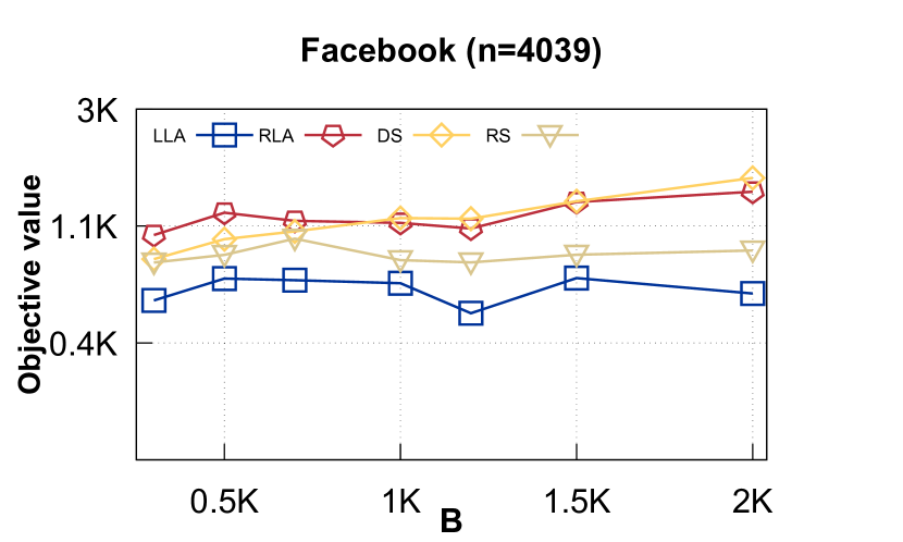
(a)

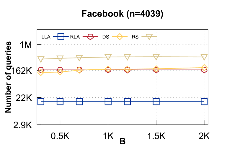
(b)

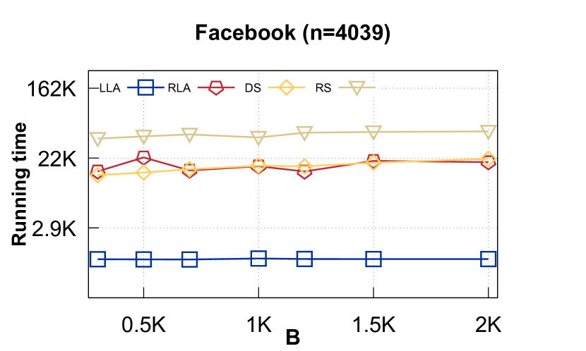
(c)

Figure 1: Algorithm results for kIMK on Facebook: (a) The objective values, (b) The number of queries, (c) Time consumption

Second, Figure 1(b)(c) displays the amounts of queries called and the time needed to run these algorithms. LAA shows an advantage over others in terms of query complexity. It is sharply from several to dozens of times lower than the remaining. Besides, the number of queries of RLA is equivalent to DS and lower than RS, respectively. Significantly, these lines explicitly determine and linear over $B$ milestones. Overall, the number of queries of RS is the highest, followed by the group of RLA-DS and LAA, respectively. The experiment indicates the quantities of queries of our algorithms outperform the others.

As the query complexity directly influences the running time, the representation of the time graph in Figure 1(c) looks quite similar to the representation of the query graph in Figure 1(b) in which LAA line was drawn typically lowest. It shows the running time of LAA is several to dozens of times faster than the others. RLA runs considerably faster than RS and equivalently to DS.

The above figures show the trade-off between our proposed algorithms’ solution qualities and the query complexities. LAA tries to target the near-optimal value by dividing the ground into two subsets according to the cost values of elements and reduces query complexity by the filtering condition of the algorithm 1. Hence, the query complexity is significantly low. Nevertheless, the performance of LAA regarding solution quality is not high. RLA enhance LAA by using LAA as an input and the decreasing constant threshold. As a result, the objective of RLA is better than LAA while the number of queries is higher but still deterministic. RLA use the threshold $\tau_{v}$ to upgrade the performance. It leads to the objective value increasing, yet the number of queries also increases. Moreover, when the ground set and $B$ value grow, the solution quality improves while running time and query complexity are linear. This is extremely important when working with big data.

Regarding kSPK.

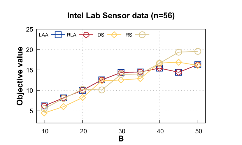
(a)

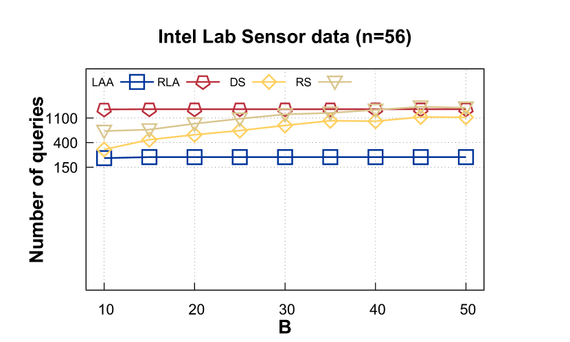
(b)

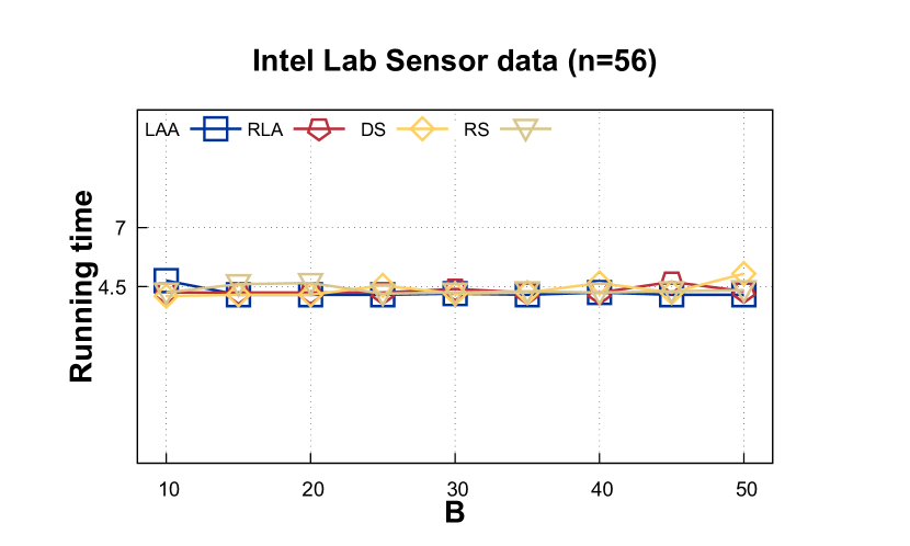
(c)

Figure 2: Algorithm results for kSPK on Intel Lab: (a) The information gained, (b) the number of queries, (c) the running time

As can be seen in 2(a) the discrimination between objective values of experimented algorithms is not large. LAA and RLA seem to overlap while DS and RS fluctuate a bit. When $B$ increases, the gap between these lines becomes larger in which RS states the highest, followed by DS and the group of LAA-RLA, respectively. However, due to the number of nodes being small, on the whole, information gained from these algorithms is almost no different.

Second, the gap between the number of queries of LAA and the others in Figure 2(b) is significantly large. With the large number of $B$, lines of RLA, DS, and RS tend convergent in which RLA lies on the remaining, followed by RS and DS, respectively. Regarding Figure 2(c), these lines seem to overlap. Moreover, query lines and timelines of the above algorithms are almost horizontal over $B$’s milestones. This result illustrates the query complexity of our algorithms is linear and equivalent to other ones.

From two actual uses of kIMK, and kSPK, our solutions are better or equivalent to existing ones while the number of queries reduces, especially when $n$ and $B$ grow. The steady of the proposed linear deterministic ones becomes vital when the data increases. The experiment showed was consistent with the theory. It also indicated the trade-off between our proposed algorithms’ solution qualities and the query complexities. Overall, our proposed algorithms are described to outperform or be comparable to the state-of-the-art.

VI Conclusion

This paper works with the problem of maximizing a $k$-submodular function under a knapsack constraint for the non-monotone case. We propose two deterministic algorithms that take just $O(kn)$ query complexity. The core of our algorithms is to keep which elements are over a given appropriate threshold and then choose among them the last elements so that the total cost does not exceed a given budget, $B>0$.

To investigate the performance of our algorithms in practice, we conducted some experiments on two applications of Influence Maximization and Sensor Placement. Experimental results have shown that our algorithms not only return acceptably reasonable solutions regarding quality requirements but also take a smaller number of queries than state-of-the-art algorithms. However, there are still some open questions, such as how to improve the approximate ratio or the linear query complexity for the $\mathsf{\mbox{non-monotone }kSMK}$ problem, that will motivate us in the future.

Appendix

VI-A The proofs of Lemmas and Theorems

Proof of Lemma 1.

Due to $f$ might be non-monotone, recap that $(e_{j},i_{j})$ is the $j$-tuple added into the candidate set x after the loop of Algorithm 1. We have 2 sub-cases:

• If $e_{j}\notin supp({\textbf{o}}_{2})$, define an integer number $l\in[k]$ that $l\neq i_{j}$ and ${\textbf{o}}^{j}_{l}$ a $k$-set such that ${\textbf{o}}^{j}_{l}(e)={\textbf{o}}^{j}_{2}(e),\forall e\in V_{2}\setminus\{e_{j}\}$ and ${\textbf{o}}^{j}_{l}(e_{j})=l$, we have:

  $$f({\textbf{o}}_{2}^{j-1})-f({\textbf{o}}_{2}^{j}) =f({\textbf{o}}^{j}_{l})-f({\textbf{o}}_{2}^{j-1})$$

  $$-(f({\textbf{o}}_{2}^{j})+f({\textbf{o}}^{j}_{l})-2f({\textbf{o}}_{2}^{j-1}))$$ (9)

  $$\leq f({\textbf{o}}^{j}_{l})-f({\textbf{o}}_{2}^{j-1})$$ (10)

  $$\leq f({\textbf{x}}^{j}_{l})-f({\textbf{x}}^{j-1})$$ (11)

  $$\leq f({\textbf{x}}^{j})-f({\textbf{x}}^{j-1})$$ (12)

  where the inequality (10) is due to the pairwise-monotoncity of $f$, the inequality (11) is due to the $k$-submodularity of $f$, and the inequality (12) is due to the selection rule of the algorithm. The proof is completed.

• If $e_{j}\in supp({\textbf{o}}_{2})$. In this case, if ${\textbf{o}}_{2}^{j-1}(e_{j})=i_{j}$. Due to the pairwise-monotone property of $f$, there exists $i^{\prime}\in[k]$ that $f({\textbf{x}}^{j-1}\sqcup(e_{j},i^{\prime}))\geq 0$. Therefore,

  $$f({\textbf{o}}_{2}^{j})-f({\textbf{o}}_{2}^{j-1})=0\leq f({\textbf{x}}^{j})-f({\textbf{x}}^{j-1})$$

  If ${\textbf{o}}_{2}^{j-1}(e_{j})\neq i_{j}$, we obtain:

  $$f({\textbf{o}}^{j-1})-f({\textbf{o}}^{j}) =2f({\textbf{o}}^{j-1})-2f({\textbf{o}}^{j-1/2})$$

  $$-(f({\textbf{o}}^{j-1})+f({\textbf{o}}^{j})-2f({\textbf{o}}^{j-1/2}))$$

  $$\leq 2f({\textbf{o}}^{j-1})-2f({\textbf{o}}^{j-1/2})$$

  $$\leq 2f({\textbf{x}}^{j})-2f({\textbf{x}}^{j-1})$$

The last inequality is due to the $k$-submodularity. Overall, we have $f({\textbf{o}}_{2}^{j-1})-f({\textbf{o}}_{2}^{j})\leq 2f({\textbf{x}}^{j})-2f({\textbf{x}}^{j-1})$. Therefore,

$$f({\textbf{o}}_{2})-f({\textbf{o}}_{2}^{t}) =\sum_{j=1}^{t}(f({\textbf{o}}^{j-1})-f({\textbf{o}}^{j}))$$

$$\leq 2\sum_{j=1}^{t}(f({\textbf{x}}^{j})-f({\textbf{x}}^{j-1}))\leq 2f({\textbf{x}}^{t})$$

The proof is completed. ∎

Proof of Lemma 2.

Recap ${\textbf{x}}={\textbf{x}}^{t}$. If $c({\textbf{x}}^{t})\leq B$, ${\textbf{x}}^{\prime}={\textbf{x}}^{t}$ and the Lemma holds. Therefore, we must consider the case $c({\textbf{x}}^{t})>B$. We get:

$$f({\textbf{x}}^{t})-f({\textbf{x}}^{Q}) =\sum_{j=Q+1}^{T}\Delta_{(e_{j},i_{j})}f({\textbf{x}}^{j-1})$$ (13)

$$\geq\sum_{j=Q+1}^{T}c(e_{j})\frac{f({\textbf{x}}^{j-1})}{B}$$ (14)

$$\geq\sum_{j=Q+1}^{T}c(e_{j})\frac{f({\textbf{x}}^{Q})}{B}$$ (15)

$$\geq c({\textbf{x}}^{\prime})\frac{f({\textbf{x}}^{Q})}{B}$$ (16)

where the inequality (14) is due to the selection rule of a tuple $(e,i_{j})$ into x according to the condition at Line 1 of Algorithm 1. The inequality (15) is due to $f(\cdot)\geq 0$.

Since ${\textbf{x}}^{\prime}$ is chosen from x so that its total cost is closest to $B$ and each element $e\in supp({\textbf{x}})$ has the cost at most $B/2$, thus:

$$c({\textbf{x}}^{\prime})>B-\frac{B}{2}\geq\frac{B}{2}$$

It implies that $f({\textbf{x}}^{t})-f({\textbf{x}}^{Q})\geq f({\textbf{x}}^{Q})/2$. Hence $f({\textbf{x}}^{Q})\leq 2f({\textbf{x}}^{t})/3$. In the other hand, due to the $k$-submodularity of $f$ we have $f({\textbf{x}}^{t})\leq f({\textbf{x}}^{Q})+f({\textbf{x}}^{\prime})$. Thus,

$$f({\textbf{x}}^{\prime})\geq f({\textbf{x}}^{t})-f({\textbf{x}}^{Q})\geq\frac{f({\textbf{x}}^{t})}{3}$$ (17)

The proof is completed. ∎

Proof of Lemma 3.

We have:

$$f({\textbf{o}}_{2})-f({\textbf{x}}^{t}) =f({\textbf{o}}_{2})-f({\textbf{o}}_{2}^{t})+f({\textbf{o}}_{2}^{t})-f({\textbf{x}}^{t})$$ (18)

$$\leq 2f({\textbf{x}}^{t})+f({\textbf{o}}_{2}^{t})-f({\textbf{x}}^{t})\ \ \ (\mbox{Due to Lemma~{}\ref{lem:1}})$$ (19)

$$\leq 2f({\textbf{x}}^{t})+\sum_{e\in supp({\textbf{o}}_{2}^{t})\setminus supp({\textbf{x}}^{t})}\Delta_{(e,i_{j}),\forall i\in[k]}f({\textbf{x}}^{t})$$ (20)

$$\leq 2f({\textbf{x}}^{t})+\sum_{e\in supp({\textbf{o}}_{2}^{t})\setminus supp({\textbf{x}}^{t})}\frac{c(e)f({\textbf{x}}^{t})}{B}$$ (21)

$$\leq 2f({\textbf{x}}^{t})+\frac{Bf({\textbf{x}}^{t})}{B}=3f({\textbf{x}}^{t})$$ (22)

where the inequality (20) is due to the $k$-submodularity of $f$, the inequality (21) is due to the selection of the algorithm. Thus, we have: $f({\textbf{o}}^{t}_{2})\leq 4f({\textbf{x}}^{t})$ or $f({\textbf{o}}^{t}_{2})\leq 4f({\textbf{x}})$. The proof is completed. ∎

Proof of Lemma 4.

Applying the Lemmas 1 and 3, with $j=t$, we have:

$$f({\textbf{o}}_{2})-f({\textbf{x}}^{t}) =f({\textbf{o}}_{2})-f({\textbf{o}}_{2}^{t})+f({\textbf{o}}_{2}^{t})-f({\textbf{x}}^{t})$$

$$\leq 2f({\textbf{x}}^{t})+f({\textbf{o}}_{2}^{t})-f({\textbf{x}}^{t})$$

$$\leq 5f({\textbf{x}}^{t})$$

Thus $f({\textbf{x}}^{t})\geq f({\textbf{o}}_{2})/6$. Combine the above implication with the Lemma 2, we have $f({\textbf{x}}^{\prime})\geq f({\textbf{x}}^{t})/3\geq f({\textbf{o}}_{2})/18$. ∎

Proof of Theorem 1.

The algorithm scans only once over the ground set, and each element $e$ has $k$ queries to find the position $i_{e}$. Therefore the number of queries is $nk$. We now prove the approximation ratio of the algorithm. By the selection of $(e_{m},i_{m})$ and the ${\textbf{o}}_{1}$ contains at most one element so $f({\textbf{o}}_{1})\leq f((e_{m},i_{m}))$. By the definition of ${\textbf{o}}_{1}^{\prime},{\textbf{o}}_{2}^{\prime}$ and the $k$-submodularity of $f$, we obtain:

$$f({\textbf{o}}) \leq f({\textbf{o}}^{\prime}_{1})+f({\textbf{o}}^{\prime}_{2})$$ (23)

$$\leq f({\textbf{o}}_{1})+f({\textbf{o}}_{2})$$ (24)

$$\leq f((e_{m},i_{m}))+18f({\textbf{x}}^{\prime})\leq 19f({\textbf{s}})$$ (25)

The proof was completed. ∎

Proof of Lemma 5.

Due to the same selection rule between $(e,i_{v})$ of Algorithm 2 and $(e,i_{e})$ of Algorithm 1, we have the same result with Lemma 1, i.e., $f({\textbf{o}})-f({\textbf{o}}^{q})\leq 2f({\textbf{s}}_{v})$. Thus:

$$f({\textbf{o}})-f({\textbf{s}}_{v}) =f({\textbf{o}})-f({\textbf{o}}^{q})+f({\textbf{o}}^{q})-f({\textbf{s}}_{v})$$ (26)

$$\leq 2f({\textbf{s}}_{v})+\sum_{j=1}^{r}(f({\textbf{u}}_{j})-f({\textbf{u}}_{j-1}))$$ (27)

$$\leq 2f({\textbf{s}}_{v})+\sum_{j=1}^{r}\Delta_{(u_{j},i_{j})}f({\textbf{s}}_{v}^{<{u_{j}}})$$ (28)

$$\leq 2f({\textbf{s}}_{v})+\sum_{j=1}^{r}c(u_{j})\tau_{v}$$ (29)

$$\leq 2f({\textbf{s}}_{v})+c({\textbf{o}})\tau_{v}$$ (30)

where the inequality (28) is due to the $k$-submodularity, the inequality (29) is due to the definition of ${\textbf{s}}_{v}^{<o}$, and the inequality (30) is due to the definition of u and o. Thus, the proof is completed.

∎

Proof of Theorem 2.

The algorithm needs $nk$ queries to call LAA and uses only 1-pass over the ground set for finishing the outer loop (Line 3-11). For each incoming element, it takes at most $k\cdot\lceil\log_{(1+\epsilon)}(19)\rceil$ queries for updating ${\textbf{s}}_{v},v\in A$. Combine all tasks, the required number of queries at most:

$$nk+nk\lceil\log_{(1+\epsilon)}(19)\rceil \leq nk+nk(1+\log_{(1+\epsilon)}(19))$$

$$=2nk+nk\frac{\ln(19)}{\ln(1+\epsilon)}$$

$$\leq 2nk+nk\frac{\ln(19)}{\ln\frac{1}{1-\frac{\epsilon}{2}}}$$

$$=2nk-nk\frac{\ln(19)}{\ln(1-\frac{\epsilon}{2})}$$

$$\leq 2nk+\frac{2}{\epsilon}nk\ln(19)=O(\frac{nk}{\epsilon})$$

We now show the approximation ratio of the algorithm. By Theorem 1, we have $\Gamma\leq{\mathsf{opt}}\leq 19.\Gamma$. Therefore, there exists an integer number $v\in A$ so that ${\mathsf{opt}}/(1+\epsilon)\leq v\leq{\mathsf{opt}}$. We have:

$$f({\textbf{s}}^{j}_{v})=\sum_{i=1}^{j}(f({\textbf{s}}^{i}_{v})-f({\textbf{s}}^{i-1}_{v}))\geq\sum_{i=1}^{j}c(e_{i})\theta_{v}=c({\textbf{s}}^{j}_{v})\theta_{v}$$ (31)

We consider the following cases:
Case 1. There exists an element $o\in supp({\textbf{o}})\setminus supp({\textbf{s}}_{v})$ so that $\Delta_{(o,{\textbf{o}}(o))}f({\textbf{s}}_{v}^{<o})\geq\tau_{v}$ and $c({\textbf{s}}_{v}^{<o})+c(o)>B$. Recall $(e_{m},i_{m})=\arg\max_{e\in V,i\in[k]}f((e,i))$, we have:

$$f({\textbf{s}}_{final}) \geq\max\{f({\textbf{s}}_{v}),f((e_{m},i_{m}))\}$$ (32)

$$\geq\max\{f({\textbf{s}}_{v}^{<o}),f((o,{\textbf{o}}(o)))\}$$ (33)

$$\geq\frac{f({\textbf{s}}_{v}^{<o})+f((o,{\textbf{o}}(o)))}{2}$$ (34)

$$\geq\frac{f({\textbf{s}}_{v}^{<o}\sqcup(o,{\textbf{o}}(o))}{2}$$ (35)

$$=\frac{\Delta_{(o,{\textbf{o}}(o))}f({\textbf{s}}_{v}^{<o})+f({\textbf{s}}^{<o}_{v})}{2}$$ (36)

$$\geq\frac{\tau_{v}c(o)+\tau_{v}c({\textbf{s}}^{o}_{v})}{2}\geq\frac{B\tau_{v}}{2}=\frac{v}{5}$$ (37)

$$\geq\frac{{\mathsf{opt}}}{5(1+\epsilon)}$$ (38)

$$\geq(\frac{1}{5}-\epsilon){\mathsf{opt}}$$ (39)

Case 2. There is no such an element $o$ like Case 1. By the Lemma 5, $c({\textbf{o}})\leq B$, $\tau_{v}=2v/(5B)$, and $f({\textbf{o}})={\mathsf{opt}}\geq v$ we have:

$$f({\textbf{o}}) \leq 3f({\textbf{s}}_{v})+B\tau_{v}\leq 3f({\textbf{s}}_{v})+2Bv/(5B)$$ (40)

$$\leq 3f({\textbf{s}}_{v})+2{\mathsf{opt}}/5$$ (41)

It implies: ${\mathsf{opt}}\leq 3f({\textbf{s}}_{v})+2{\mathsf{opt}}/5$, thus ${\mathsf{opt}}\leq 5f({\textbf{s}}_{v})$. Finally, $f({\textbf{s}}_{final})\geq f({\textbf{s}}_{v})\geq{\mathsf{opt}}/5$. By combining the two above cases, we obtain the proof. ∎

References

- [1] L. Lovász, “Submodular functions and convexity,” in Mathematical Programming The State of the Art, XIth International Symposium on Mathematical Programming, Bonn, Germany, August 23-27, 1982, A. Bachem, B. Korte, and M. Grötschel, Eds. Springer, 1982, pp. 235–257.
- [2] A. P. Singh, A. Guillory, and J. A. Bilmes, “On bisubmodular maximization,” in In Proc. of the International Conference on Artificial Intelligence and Statistics (AISTATS), 2012, pp. 1055–1063.
- [3] J. Ward and S. Zivný, “Maximizing bisubmodular and k-submodular functions,” in In Proc. of Symposium on Discrete Algorithms (SODA), 2014, pp. 1468–1481.
- [4] Y. Zhang, M. Li, D. Yang, and G. Xue, “A budget feasible mechanism for k-topic influence maximization in social networks,” in In Proc. of IEEE Global Communications Conference (GLOBECOM), 2019, pp. 1–6.
- [5] N. Ohsaka and Y. Yoshida, “Monotone k-submodular function maximization with size constraints,” in In Proc. of Annual Conference on Neural Information Processing Systems (NIPS), 2015, pp. 694–702.
- [6] A. Rafiey and Y. Yoshida, “Fast and private submodular and k-submodular functions maximization with matroid constraints,” in In Proc. of the International Conference on Machine Learning (ICML), 2020, pp. 7887–7897.
- [7] C. Qian, J. Shi, K. Tang, and Z. Zhou, “Constrained monotone k-submodular function maximization using multiobjective evolutionary algorithms with theoretical guarantee,” IEEE Trans. Evol. Comput., vol. 22, no. 4, pp. 595–608, 2018.
- [8] L. Nguyen and M. Thai, “Streaming k-submodular maximization under noise subject to size constraint,” in In Proc. of the International Conference on Machine Learning (ICML), 2020, pp. 7338–7347.
- [9] Z. Wang, E. Chen, Q. Liu, Y. Yang, Y. Ge, and B. Chang, “Maximizing the coverage of information propagation in social networks,” in Proceedings of the Twenty-Fourth International Joint Conference on Artificial Intelligence, IJCAI 2015, Buenos Aires, Argentina, July 25-31, 2015, Q. Yang and M. J. Wooldridge, Eds. AAAI Press, 2015, pp. 2104–2110.
- [10] C. Qian, J. Shi, K. Tang, and Z. Zhou, “Constrained monotone k-submodular function maximization using multiobjective evolutionary algorithms with theoretical guarantee,” IEEE Trans. Evol. Comput., vol. 22, no. 4, pp. 595–608, 2018.
- [11] C. V. Pham, D. T. Ha, H. X. Hoang, and T. D. Tran, “Fast streaming algorithms for -submodular maximization under a knapsack constraint,” in The 9th IEEE International Conference on Data Science and Advanced Analytics, 2022.
- [12] D. Kempe, J. M. Kleinberg, and É. Tardos, “Maximizing the spread of influence through a social network,” in In Proc. of the International Conference on Knowledge Discovery and Data Mining (KDD), 2003, pp. 137–146.
- [13] “On maximizing a monotone k-submodular function under a knapsack constraint,” Operations Research Letters, vol. 50, no. 1, pp. 28–31, 2022.
- [14] B. Wang and H. Zhou, “Multilinear extension of k-submodular functions,” CoRR, vol. abs/2107.07103, 2021. [Online]. Available: https://arxiv.org/abs/2107.07103
- [15] U. Feige, V. S. Mirrokni, and J. Vondrák, “Maximizing non-monotone submodular functions,” SIAM J. Comput., vol. 40, no. 4, pp. 1133–1153, 2011.
- [16] N. Buchbinder, M. Feldman, and R. Schwartz, “Comparing apples and oranges: Query tradeoff in submodular maximization,” in Proceedings of the Twenty-Sixth Annual ACM-SIAM Symposium on Discrete Algorithms, SODA 2015, San Diego, CA, USA, January 4-6, 2015, P. Indyk, Ed. SIAM, 2015, pp. 1149–1168.
- [17] B. Mirzasoleiman, A. Badanidiyuru, and A. Karbasi, “Fast constrained submodular maximization: Personalized data summarization,” in In Proc. of the International Conference on Machine Learning (ICML), vol. 48, 2016, pp. 1358–1367.
- [18] C. V. Pham, Q. C. Vu, D. K. Ha, T. T. Nguyen, and N. D. Le, “Maximizing k-submodular functions under budget constraint: applications and streaming algorithms,” J. Comb. Optim., vol. 44, no. 1, pp. 723–751, 2022.
- [19] S. Iwata, S. Tanigawa, and Y. Yoshida, “Improved approximation algorithms for k-submodular function maximization,” in Proceedings of the Twenty-Seventh Annual ACM-SIAM Symposium on Discrete Algorithms, SODA 2016, R. Krauthgamer, Ed. SIAM, 2016, pp. 404–413.
- [20] H. Oshima, “Derandomization for k-submodular maximization,” in In Proc. of International Workshop Combinatorial Algorithms (IWOCA), L. Brankovic, J. Ryan, and W. F. Smyth, Eds., 2017, pp. 88–99.
- [21] S. Sakaue, “On maximizing a monotone k-submodular function subject to a matroid constraint,” Discret. Optim., vol. 23, pp. 105–113, 2017.
- [22] A. Rafiey and Y. Yoshida, “Fast and private submodular and k-submodular functions maximization with matroid constraints,” in In Proc. of International Conference on Machine Learning (ICML), 2020, pp. 7887–7897.
- [23] T. Soma, “No-regret algorithms for online k-submodular maximization,” in In Proc. of International Conference on Artificial Intelligence and Statistics (AISTATS), 2019, pp. 1205–1214.
- [24] A. Ene and H. L. Nguyen, “Streaming algorithm for monotone k-submodular maximization with cardinality constraints,” in ICML 2022, ser. Proc. of MLR, vol. 162. PMLR, 2022, pp. 5944–5967.
- [25] E. Balkanski, S. Qian, and Y. Singer, “Instance specific approximations for submodular maximization,” in Proc. of the 38th ICML 2021, ser. Proceedings of Machine Learning Research, vol. 139. PMLR, 2021, pp. 609–618.
- [26] M. Sviridenko, “A note on maximizing a submodular set function subject to a knapsack constraint,” Oper. Res. Lett., vol. 32, no. 1, pp. 41–43, 2004.
- [27] J. Leskovec and Krevl, “A. snap datasets: Stanford large network dataset collection,” 2014. [Online]. Available: http://snap. stanford.edu/data
- [28] P. Bodik, W. Hong, C. Guestrin, S. Madden, M. Paskin, and R. Thibaux, “Intel lab,” 2004. [Online]. Available: http://db.csail.mit.edu/labdata/labdata.html
- [29] W. Chen, Y. Yuan, and L. Zhang, “Scalable influence maximization in social networks under the linear threshold model,” in In Proc. of IEEE International Conference on Data Mining (ICDM), 2010, pp. 88–97.
- [30] C. Borgs, M. Brautbar, J. T. Chayes, and B. Lucier, “Maximizing social influence in nearly optimal time,” in In Proc. of Symposium on Discrete Algorithms (SODA), 2014, pp. 946–957.