Singular Control in a Cash Management Model with Ambiguity

Abstract

We consider a singular control model of cash reserve management, driven by a diffusion under ambiguity. The manager is assumed to have maxmin preferences over a set of priors characterized by $\kappa$-ignorance. A verification theorem is established to determine the firm’s cost function and the optimal cash policy; the latter taking the form of a control barrier policy. In a model driven by arithmetic Brownian motion, we numerically show that an increase in ambiguity leads to higher expected costs under the worst-case prior and a narrower inaction region. The latter effect can be used to provide an ambiguity-driven explanation for observed cash management behavior.

Keywords: Singular control, Ambiguity, Inventory models

1 Introduction

An important question in corporate finance is that of optimal cash management. On the one hand, firms require cash to finance the firm as a going concern. On the other hand, shareholders require dividend payouts as a reward for providing capital. The seminal contribution by Jeanblanc-Picqué and Shiryaev, (1995) uses a stochastic storage models à la Harrison and Taksar, (1978) to find the optimal size of a firm’s cash hoard in the face of stochastically evolving net cash flows. In this paper, we are interested in optimal cash management under ambiguity, i.e., a situation where the manager is not able to reduce the uncertainty over future net cash flows into a single probability measure. We are interested in the interplay between traditional concerns over risk (as measured by, e.g., confidence intervals provided by a given probability measure) and ambiguity (as measured by the “size” of the set of probability measures considered by the manager) under the assumption that the manager is ambiguity averse.

Our motivation for including ambiguity in a model of optimal cash holding is the finding from the recent literature that shows that decision makers’ beliefs influence corporate cash holdings. In particular, Deshmukh et al., (2021) show that “relative to rational CEOs, optimistic CEOs hold 24% less cash.” In a standard Bayesian setting this can only be explained if different CEOs use different probability measures. This then almost inevitably leads to one CEO being “more rational” than another. From a theoretical perspective this is unsatisfactory. For example, in Deshmukh et al., (2021) there is a “true” probability measure which then gets distorted by non-rational optimistic or pessimistic CEOs. We propose to use a framework in which all managers may use the same reference prior over future cash flows, but they may differ in their level of ambiguity over the true probability measure, e.g., due to differing levels of experience in their industry.

The distinction between uncertainty resulting from randomness governed by a distribution (“known unknowns”) and uncertainty over the correct distribution (“unknown unknowns”) goes back to Knight, (1921). In his seminal work he refers to the former as risk and the latter as uncertainty or ambiguity.

The effect of ambiguity on decision making has been studied extensively, most famously by Ellsberg, (1961). The overwhelming conclusion of the experimental literature is that decision makers are ambiguity averse. In the classical Ellsberg experiment, a DM has to place bets on one of two urns, both with 100 red or blue balls. For the first urn it is known that half the balls are red. For the second urn no such information is available. Since most people are observed to choose bets on the first urn over bets on the second urn, Savage’s “sure thing principle” is being violated.

Note that the Ellsberg paradox is not really a paradox, because it does not result from a cognitive bias or irrationality. Rather, observed behaviour is driven by a lack of information. It is perfectly possible for DMs to make consistent decisions under ambiguity. This has been shown by Gilboa and Schmeidler, (1989), who incorporate an ambiguity aversion axiom into the subjective expected utility framework. They then show that a rational decision maker acts as if she maximizes expected utility over the worst–case prior within a (subjectively chosen) set of priors. This approach has been successfully used in many applications in economics, finance, and OR.

Our contribution is to apply the maxmin multiple prior model to a singular control model of optimal storage inventory, with an application to a firm’s cash management. On a regular basis, firms are faced with operational costs (e.g. rent, capital stock, labour’s wage, etc.) that have to be settled promptly with reserved cash. The fact that this cash generates no (or low) return means holding it results in an opportunity loss, which can be interpreted as a holding cost as it could potentially be used for income-generating activities, such as investments or paying out dividends. Therefore, excessive cash holding is undesirable. On the other hand, having a shortage of cash reserves results in a delay of cost settlement, which often incurs a penalty fee. Therefore, the firm has an incentive to inject some amount of cash into the system. This could, for example, be done by selling some assets or issuing bonds. These two circumstances create a trade-off that suggests the existence of target level of cash. In a model where cash adjustments are costly, we show that there exists an optimal control band policy, where the firm keeps its cash hoard between an upper and lower bound. While this is no different from a standard model under risk, ambiguity does bring some new aspects to the comparative statics of the optimal policy. For example, as in the standard model without ambiguity, the higher the risk, the higher the long-term discounted cost of cash. Ambiguity amplifies this effect, even though an increase in the degree of ambiguity leads to manager to exert control earlier. This is in contrast to the risk-only model, where an increase in risk leads the manager to exert control later. The reason for this result is that a more ambiguous DM expects the cash level to increase (when positive) or decrease (when negative) more rapidly (in expectation) than a less ambiguous DM. Since holding costs are increasing in the absolute value of the cash hoard, a more ambiguous DM will, thus, exert control sooner. This can provide an explanation for the empirically observed behaviour in Deshmukh et al., (2021) that “more optimistic” CEOs have bigger cash hoards. In our model, this behaviour is not due to irrationality, but an aspect of the uncertain environment that the manager faces.

The cash reserve problem was first addressed in the literature by Baumol, (1952) and Tobin, (1956), who studied the cash balance problem under the assumption that demand is deterministic, which is far from realistic. The stochastic treatment was later established under a discrete-time (Markov chain) framework by e.g. Eppen and Fama, (1969). A more general approach for storage systems in continuous time, in particular, with demand driven by Brownian motion, has been developed over the past decades. Bather, (1966), Vial, (1972), Constantinides, (1976), Harrison, (1978), Harrison and Taksar, (1983) and many others are among the notable authors. To get an overview of the related papers, we refer the reader to Harrison, (2013).

One of the first papers to axiomatize ambiguity is Gilboa and Schmeidler, (1989). They model ambiguity as a set of priors, among which the DM (subjectively) selects the one that maximises the DM’s expected utility. Under an axiom of ambiguity aversion, the prior that is chosen is called the worse-case prior, which captures the intuition that an ambiguity-averse DM is cautious about their beliefs and heavily weighs the possibility of undesirable consequences of their decision. The Gilboa – Schmeidler criterion has become known as maxmin utility. However, the Gilboa – Schmeidler framework is a static one and is, thus, insufficient for dealing with situations where the worst-case prior might change over time. An inter-temporal version was proposed by Epstein and Wang, (1994) in discrete time and by Chen and Epstein, (2002) in continuous time. In these models, the worst-case prior is updated in a Bellman principle-like one-step-ahead procedure. In order to make this work, attention is restricted to sets of priors that are called strongly rectangular. We use the Chen and Epstein, (2002) approach to modeling multiple priors.

In fact, we use a stronger assumption, also introduced in Chen and Epstein, (2002), and assume that ambiguity takes form of $\kappa$-ignorance. That is to say, the DM has a reference probability, which is distorted through a density generator. The density generator is assumed to take values in an interval $[-\kappa,\kappa]$, so that the reference prior together with the parameter $\kappa$ determines the set of priors that is considered by the DM. While restrictive, an advantage of this approach is that the degree of ambiguity can be seen to be measured by $\kappa$.

Importantly, in our model the worst-case prior is not constant but varies over time, depending on the evolution of the actual amount of cash currently held. This unusual feature has been observed by Cheng and Riedel, (2013) in the context of pricing a straddle option and Hellmann and Thijssen, (2018). The latter paper models a timing game between two firms contemplating an investment opportunity under ambiguity and show that ambiguity aversion has two effects: ambiguity over future demand (fear of the market), as in the standard literature, but also ambiguity over the other firm’s investment decision (fear of the competitor). These have opposite effects on what constitutes the worst-case prior. It turns out there is a threshold to distinguish which type of ambiguity dominates through time. Our model has a similar feature in that control costs are incurred whether at the upper or lower barrier. The worst-case priors at each of these barriers are opposite and this leads, in turn, to the existence of a threshold somewhere in the inaction region (endogenously determined) that separates two regions where different measures constitute the worst-case prior.

The most closely contribution to our work is Chakraborty et al., (2021) in which a one-side singular control of a firm’s dividend payout policy is considered under ambiguity. They assume, in addition to the classical singular control, that there is a penalty cost associated with a change of measure, which is determined by the Kullback-Leibler divergence. The use of Kullback-Leibler divergence as a model for multiple priors is well-established in the literature on robust control; see, e.g., Hansen et al., (2006); Hansen and Sargent, (2010, 2011); Hansen and Miao, (2018, 2022); Ferrari et al., (2022) and references therein. The more behavioral approach that motivates $\kappa$-ignorance is, in fact, closely related to the robust control approach. In both cases, the solution to the control problem takes the form of a control band policy. However, it is important to note that in a robust control framework, the DM chooses a probability measure, while acknowledging the possibility of mis-specification. As a result, the DM assigns a higher weight to the cost function using an uncertainty equivalent expectation. In our work, on the other hand, the worst-case prior follows from the chosen control policy.

The structure of this paper is as follows: In Section 2 we construct a general formulation for singular control of the Brownian cash reserve under ambiguity. We provide a verification theorem for the optimal control band policy and the existence of the ambiguity trigger in Section 3. In Section 4 we provide a simplification of the verification theorem for the case where the present value of the (uncontrolled) expected holding costs is affine in the current value of the cash holdings. This includes, e.g., the case where the uncontrolled cash process follows an arithmetic Brownian motion, or a mean-reverting Ornstein-Uhlenbeck process. A numerical illustration for the arithmetic Brownian motion case is given in Section 5.

2 Simple Cash-Management Model with Drift Ambiguity

Let $E\subseteq\mathds{R}$ be a connected state space endowed with the Euclidean topology and such that $0\in E$. Given $(\Omega,{\mathscr{F}})$ a measurable space on which we define, for all $x\in E$, a probability measure $\textsf{P}_{x}$ with associated expectation operator $\textsf{E}_{x}$. On $(\Omega,{\mathscr{F}},\textsf{P}_{x})$, we assume that $\alpha:E\to\mathds{R}$ and $\sigma:E\to\mathds{R}$ are continuously differentiable functions such that

$$|\alpha(x)|+|\sigma(x)| \leq C(1+|x|)\;\;\text{for all }x\in E$$ (1)

for some $C\in\mathds{R}$. Then a time-homogeneous diffusion, $X\triangleq\left(X_{t}\right)_{t\geq 0}$, taking values in $E$, is the unique strong solution to the stochastic differential equation (SDE),

$$\mathrm{d}X_{t}=\alpha(X_{t})\mathrm{d}t+\sigma(X_{t})\mathrm{d}B_{t},\quad X_{0}=x,\quad\textsf{P}_{x}-\text{a.s.},$$ (2)

where $B\triangleq\left(B_{t}\right)_{t\geq 0}$ is a standard Brownian motion. Dynamic revelation of information is modeled by the natural filtration ${\mathbf{F}}=\left({\mathscr{F}}_{t}\right)_{t\geq 0}$ generated by $X$. We assume that the end points of $E$ are $\textsf{P}_{x}$-a.s. unattainable.

A control policy is a pair of processes $(L,U)$, where $L$ and $U$ are adapted, non-decreasing, and non-negative. These processes are associated with increases and decreases, respectively, of $X$ at times at which control is exerted. With the policy $(L,U)$ we associate the controlled process $X^{L,U}$ and we say that a control policy $(L,U)$ is feasible if for all $x\in E$, there exists a unique $X^{L,U}$ that strongly solves

$$\mathrm{d}X^{L,U}_{t}=\alpha(X^{L,U}_{t})\mathrm{d}t+\sigma(X^{L,U}_{t})\mathrm{d}B_{t}+\mathrm{d}L_{t}-\mathrm{d}U_{t}\quad X_{0}=x,\quad\textsf{P}_{x}-\text{a.s.},$$ (3)

and if there exist $A>0$ and $B<0$, such that

$$\textsf{P}_{x}\left(\sup_{t\geq 0}X^{L,U}_{t}<A,\inf_{t\geq 0}X^{L,U}_{t}>B\right) =1$$ (4)

The set of feasible control policies is denoted by ${\mathscr{D}}$, while we denote by $X^{0}$, the uncontrolled process; that is, $X^{0}\triangleq X^{0,0}$.

The instantaneous holding costs are given by an almost everywhere differentiable function $c:\mathds{R}\to\mathds{R}_{+}$. For simplicity we will assume that

$$c(x)=\begin{cases}\hat{c}|x|&\text{if $x\geq 0$}\\ \check{c}|x|&\text{if $x<0$.}\end{cases}$$ (5)

for some $\hat{c},\check{c}>0$. The instantaneous and proportional costs of lower and upper control are denoted by $\ell>0$ and $u>0$, respectively. Our results can easily be extended to more general convex holding costs with $c(0)=0$, albeit at the cost of more cumbersome notation. In a cash management setting, one could think of 0 as the target level of cash. When $x>0$, the firm has excess cash while if $x<0$ the firm needs to access cash on the markets. When the cash reserves get too low the firm may need to issue new equity, which incurs costs $\ell$, whereas when $x$ gets too large, the firm may wish to pay out dividends, which incurs a cost $u$.

The decision-maker (DM) discounts costs at the constant rate $\rho>0$. We, furthermore, assume that

$$\textsf{E}_{x}\left[\int_{0}^{\infty}e^{-\rho t}|X^{0}_{t}|\mathrm{d}t\right]<\infty,\;\;\;x\in E.$$

A typical process that satisfies all the assumptions made so far is the arithmetic Brownian motion, defined on the state space $E=\mathds{R}$, being the strong solution of the SDE

$$\mathrm{d}X^{0}_{t}=\alpha\mathrm{d}t+\sigma\mathrm{d}B_{t},$$ (6)

with constant drift $\alpha\in\mathds{R}$ and standard deviation $\sigma>0$. For this specification the uncontrolled cash process is

$$X^{0}_{t}=x+\alpha t+\sigma B_{t},$$

whereas for any feasible control policy $(L,U)\in{\mathscr{D}}$, the controlled cash process satisfies

$$X^{L,U}_{t}=x+\alpha t+\sigma B_{t}+L_{t}-U_{t}.$$

Another process that can be used is the mean-reverting Ornstein-Uhlenbeck process

$$\mathrm{d}X^{0}_{t}=-\eta X^{0}_{t}\mathrm{d}t+\sigma\mathrm{d}B_{t},$$

where $\eta>0$ is the speed of mean-reversion. In this case

$$X^{0}_{t}=xe^{-\eta t}+\int_{0}^{t}e^{-\eta(t-s)}\mathrm{d}B_{s}.$$

It is assumed that the DM is ambiguous about the measure $\textsf{P}_{x}$ and, consequently, considers a set of priors $\mathscr{P}^{\Theta}$. Each of these priors is constructed from the reference measure $\textsf{P}_{x}$ by means of a density generator $\theta\in\Theta$. A process $\theta=\left(\theta_{t}\right)_{t\geq 0}$ is a density generator if the process $\left(M^{\theta}_{t}\right)_{t\geq 0}$, with

$$\frac{\mathrm{d}M_{t}^{\theta}}{M_{t}^{\theta}}=-\theta_{t}\mathrm{d}B_{t},\quad M_{0}^{\theta}=1,$$ (7)

is a $\textsf{P}_{x}$–martingale. Such a process $\theta$ generates a new measure $\textsf{P}_{x}^{\theta}$ on $(\Omega,{\mathscr{F}}^{B})$ via the Radon–Nikodym derivative $\mathrm{d}\textsf{P}_{x}^{\theta}/\mathrm{d}\textsf{P}_{x}\big{|}_{{\mathscr{F}}^{B}_{T}}=M^{\theta}_{T}$ for any $T>0$. Here, ${\mathscr{F}}^{B}\triangleq{\mathscr{F}}^{B}_{\infty}$, where ${\mathbf{F}}^{B}\triangleq\left({\mathscr{F}}^{B}_{t}\right)_{t\geq 0}$ is the (uncompleted) filtration generated by $B$. Indeed, if $\theta\in\Theta$, then it follows from Girsanov’s theorem (see, Corollary 5.2 in Chapter 3.5 of Karatzas and Shreve,, 1991) that under the measure $\textsf{P}_{x}^{\theta}$ the process $B^{\theta}\triangleq\left(B^{\theta}_{t}\right)_{t\geq 0}$, defined by

$$B^{\theta}_{t}\triangleq B_{t}+\int_{0}^{t}\theta_{s}\mathrm{d}s,$$

is a Brownian motion on $(\Omega,{\mathscr{F}}^{B},{\mathbf{F}}^{B},\textsf{P}^{\theta}_{x})$ and that, under $\textsf{P}_{x}^{\theta}$, the process $X^{L,U}$ is the unique strong solution to the SDE

$$\mathrm{d}X^{L,U}_{t}=\big{(}\alpha(X^{L,U}_{t})-\sigma(X^{L,U}_{t})\theta_{t}\big{)}\mathrm{d}t+\sigma(X^{L,U}_{t})\mathrm{d}B^{\theta}_{t}+\mathrm{d}L_{t}-\mathrm{d}U_{t},\quad\textsf{P}_{x}^{\theta}(X^{L,U}_{0}=x)=1.$$

In the remainder we restrict attention to so-called $\kappa$-ignorance, i.e. we only use density generators $\theta$ for which $\theta_{t}\in[-\kappa,+\kappa]$ for all $t\geq 0$ and some $\kappa\geq 0$. Note that $\mathscr{P}^{\Theta}=\{\textsf{P}_{x}\}$ if $\kappa=0$.

To model ambiguity aversion, it is assumed that the DM uses maxmin utility à la Gilboa and Schmeidler, (1989). That is, the worst-case cost function associated with the feasible policy $(L,U)\in{\mathscr{D}}$ is given by $J^{L,U}:E\to\mathds{R}$, where

$$J^{L,U}(x)\triangleq\sup_{\theta\in\Theta}\textsf{E}^{\theta}_{x}\left[\int_{0}^{\infty}e^{-\rho t}\left(c(X^{L,U}_{t})\mathrm{d}t+\ell\mathrm{d}L_{t}+u\mathrm{d}U_{t}\right)\right].$$ (8)

The DM’s objective is to find the feasible policy that minimizes the worst-case expected costs over the set of priors ${\mathscr{P}}^{\Theta}$. The firm’s minimal cost function is

$$J^{\ast}(x)\triangleq\inf_{(L,U)\in{\mathscr{D}}}J^{L,U}(x).$$ (9)

From Chen and Epstein, (2002, Theorem 2.1) it follows that there exists an upper-rim generator $\theta^{\ast}\in\Theta$ so that

$$J^{L,U}(x)=\textsf{E}^{\theta^{\ast}}_{x}\left[\int_{0}^{\infty}e^{-\rho t}\left\{c\left(X^{L,U}_{t}\right)\mathrm{d}t+\ell\mathrm{d}L_{t}+u\mathrm{d}U_{t}\right\}\right].$$ (10)

Furthermore, from Chen and Epstein, (2002, Section 3.3) it follows that under $\kappa$-ignorance it holds that $\theta^{\ast}_{t}\in\{-\kappa,\kappa\}$ for all $t\geq 0$.

Finally, in many cases the optimal policy consists of exerting control only when the process $X$ exits an interval $({\underline{x}},{\overline{x}})$. Therefore, with each pair $({\underline{x}},{\overline{x}})\in E\times E$, ${\underline{x}}<{\overline{x}}$, we associate the control band policy $(L,U)\in{\mathscr{D}}$ for which ${\underline{x}}$ is an (upward) reflecting barrier for $L$ and ${\overline{x}}$ is a (downward) reflecting barrier for $U$. For such policies it holds that

1. $X^{L,U}_{t}\in[{\underline{x}},{\overline{x}}]$, $\textsf{P}_{x}$-a.s. for all $t\geq 0$, and

2. $\int_{0}^{\infty}1_{({\underline{x}},{\overline{x}})}(X^{L,U}_{t})\mathrm{d}(L_{t}+U_{t})=0$, $\textsf{P}_{x}$-a.s.

Following Tanaka, (1979), our assumptions on $X$ are sufficient to guarantee the existence of control band policies.

3 A General Verification Theorem

Let ${\mathscr{L}}$ denote the characteristic operator on $C^{2}(E)$ of the killed process $\big{(}e^{-\rho t}X_{t}\big{)}_{t\geq 0}$ under $\textsf{P}_{x}$, i.e.

$${\mathscr{L}}\varphi(x)=\frac{1}{2}\sigma^{2}(x)\varphi^{\prime\prime}(x)+\alpha(x)\varphi^{\prime}(x)-\rho\varphi(x).$$ (11)

On $C^{1}(E)$ we also define the density generator,

$$\theta^{\varphi}\triangleq\theta^{\varphi}(x)\triangleq\begin{cases}-\kappa&\text{if $\varphi^{\prime}(x)\geq 0$}\\ +\kappa&\text{if $\varphi^{\prime}(x)<0$.}\end{cases}$$

We get the following verification theorem.

Theorem 1.

Suppose there exists a pair $({\underline{x}},{\overline{x}})\in E\times E$, ${\underline{x}}<0<{\overline{x}}$, and a non-negative, convex, and $C^{2}$-function $\varphi$ on $({\underline{x}},{\overline{x}})$ such that

1. $\theta^{\varphi}(x)\sigma(x)\varphi^{\prime}(x)-{\mathscr{L}}\varphi(x)=c(x)$ on $({\underline{x}},{\overline{x}})$,

2. $\varphi^{\prime}({\underline{x}}+)=-\ell$, $\varphi^{\prime}({\overline{x}}-)=u$,

3. $\varphi^{\prime\prime}({\underline{x}}+)=\varphi^{\prime\prime}({\overline{x}}-)=0$,

4. $\check{c}|x-{\underline{x}}|\geq\ell\big{[}\rho|{\underline{x}}-x|-\big{(}\alpha(x)-\alpha({\underline{x}})\big{)}-\kappa\big{(}\sigma(x)-\sigma({\underline{x}})\big{)}\big{]}$, for all $x<{\underline{x}}$,

5. $\hat{c}|x-{\overline{x}}|\geq u\big{[}\rho|{\overline{x}}-x|-\big{(}\alpha({\overline{x}})-\alpha(x)\big{)}+\kappa\big{(}\sigma({\overline{x}})-\sigma(x)\big{)}\big{]}$, for all $x>{\overline{x}}$, and

6. $\lim_{T\to\infty}e^{-\rho T}\textsf{E}_{x}^{\theta^{\varphi}}\left[\varphi\big{(}X_{s}^{L,U}\big{)}\right]=0$, for all $(L,U)\in{\mathscr{D}}$.

Then the optimal policy $(L^{\ast},U^{\ast})$ is the control band policy associated with $({\underline{x}},{\overline{x}})$ and the minimal cost function is

$$J^{\ast}(x)=\begin{cases}\ell|{\underline{x}}-x|+\varphi({\underline{x}}+)&\text{if $x\leq{\underline{x}}$}\\ \varphi(x)&\text{if ${\underline{x}}<x<{\overline{x}}$}\\ u|x-{\overline{x}}|+\varphi({\overline{x}}-)&\text{if $x\geq{\overline{x}}$}\end{cases}.$$

Remark 1.

Conditions 4 and 5 guarantee existence of a feasible policy under ambiguity. For the case of an uncontrolled arithmetic Brownian motion,

$$\mathrm{d}X^{0}=\alpha\mathrm{d}t+\sigma\mathrm{d}B_{t},$$

these conditions reduce to

$$\check{c}\geq\rho\ell,\quad\text{and}\quad\hat{c}\geq\rho u.$$

That is, the discounted perpetual holding costs of positive (negative) cash balances should exceed the control costs of reducing (increasing) the cash balance. As another example, for the case of an uncontrolled mean-reverting Ornstein-Uhlenbeck process,

$$\mathrm{d}X^{0}=\eta(\tilde{x}-X^{0}_{t})\mathrm{d}t+\sigma\mathrm{d}B_{t},$$

where $\tilde{x}$ is the long-run mean and $\eta$ is the speed of mean reversion, conditions 4 and 5 reduce to

$$\check{c}\geq(\rho+\eta)\ell,\quad\text{and}\quad\hat{c}\geq(\rho+\eta)u.$$

Proof. Let $\varphi$ and ${\underline{x}}<0<{\overline{x}}$ satisfy conditions 1–6. Extend $\varphi$ to $E$, in a twice-continuously differentiable way, as follows:

$$\varphi(x)=\begin{cases}\ell|{\underline{x}}-x|+\varphi({\underline{x}}+)&\text{if $x\leq{\underline{x}}$}\\ \varphi(x)&\text{if ${\underline{x}}<x<{\overline{x}}$}\\ u|x-{\overline{x}}|+\varphi({\overline{x}}-)&\text{if $x\geq{\overline{x}}$}\end{cases}.$$

Let $(L^{\ast},U^{\ast})$ be the control band policy associated with $({\underline{x}},{\overline{x}})$. The proof proceeds in two steps. First we prove that $J^{L^{\ast},U^{\ast}}=\varphi$. Then we show that for any other feasible policy $(L,U)$ it holds that $J^{L,U}\geq J^{L^{\ast},U^{\ast}}$, so that $J^{\ast}=J^{L^{\ast},U^{\ast}}$. Note that

$$\theta^{\varphi}(x)={\arg\min}_{\theta\in[-\kappa,+\kappa]}\big{(}\theta\sigma(x)\text{sign}(\varphi^{\prime}(x))\big{)},$$ (12)

so that the worst-case prior is generated by

$$\theta^{\ast}_{t}(\omega)=\theta^{\varphi}\big{(}X_{t}(\omega)\big{)}.$$ (13)

1. Fix $T>0$, $x\in E$, $\theta\in\Theta$ and set $\theta^{\varphi}_{t}\triangleq\theta^{\varphi}(X^{L^{\ast},U^{\ast}}_{t})$. From Itō’s lemma it then follows that

$$\textsf{E}^{\theta}_{x}\left[e^{-\rho T}\varphi\big{(}X^{L^{\ast},U^{\ast}}_{T}\big{)}\right]= \varphi(x)+\textsf{E}^{\theta}_{x}\left[\int_{0}^{T}e^{-\rho s}\varphi^{\prime}\big{(}X^{L^{\ast},U^{\ast}}_{s}\big{)}\mathrm{d}\left(L^{\ast}_{s}+U^{\ast}_{s}\right)\right]$$

$$+\textsf{E}^{\theta}_{x}\left[\int_{0}^{T}e^{-\rho s}\left\{{\mathscr{L}}\varphi\big{(}X^{L^{\ast},U^{\ast}}_{s}\big{)}-\theta_{s}\sigma\big{(}X^{L^{\ast},U^{\ast}}_{s}\big{)}\varphi^{\prime}\big{(}X^{L^{\ast},U^{\ast}}_{s}\big{)}\right\}\mathrm{d}s\right]$$

$$\leq \varphi(x)+\textsf{E}^{\theta}_{x}\left[\int_{0}^{T}e^{-\rho s}\varphi^{\prime}\big{(}X^{L^{\ast},U^{\ast}}_{s}\big{)}\mathrm{d}\left(L^{\ast}_{s}+U^{\ast}_{s}\right)\right]$$

$$+\textsf{E}^{\theta}_{x}\left[\int_{0}^{T}e^{-\rho s}\left\{{\mathscr{L}}\varphi\big{(}X^{L^{\ast},U^{\ast}}_{s}\big{)}-\theta^{\varphi}_{s}\sigma\big{(}X^{L^{\ast},U^{\ast}}_{s}\big{)}\varphi^{\prime}\big{(}X^{L^{\ast},U^{\ast}}_{s}\big{)}\right\}\mathrm{d}s\right]$$

$$= \varphi(x)-\textsf{E}_{x}^{\theta}\left[\int_{0}^{T}e^{-\rho s}c\left(X_{s}^{L^{\ast},U^{\ast}}\right)\mathrm{d}s+\int_{0}^{T}e^{-\rho s}\left(u\mathrm{d}U^{\ast}_{s}+\ell\mathrm{d}L^{\ast}_{s}\right)\right],$$

where the inequality follows from  (12) and  (13), and the final equality follows from conditions 1 and 2.

Sending $T\to\infty$ and exploiting the non-negativity of $\varphi$, $c$, $u$, and $\ell$, we find that

$$\varphi(x) \geq\textsf{E}_{x}^{\theta}\left[\int_{0}^{\infty}e^{-\rho s}c\left(X_{s}^{L^{\ast},U^{\ast}}\right)\mathrm{d}s+\int_{0}^{\infty}e^{-\rho s}\left(u\mathrm{d}U^{\ast}_{s}+\ell\mathrm{d}L^{\ast}_{s}\right)\right].$$

Since $\theta\in\Theta$ was chosen arbitrarily, this implies that

$$\varphi(x) \geq\inf_{(L,U)\in{\mathscr{D}}}\sup_{\theta\in\Theta}\textsf{E}_{x}^{\theta}\left[\int_{0}^{\infty}e^{-\rho s}c\left(X_{s}^{L,U}\right)\mathrm{d}s+\int_{0}^{\infty}e^{-\rho s}\left(u\mathrm{d}U_{s}+\ell\mathrm{d}L_{s}\right)\right].$$

2. Next, note that Conditions 4 and 5 ensure that

$$\theta^{\varphi}({\underline{x}})\sigma(x)\varphi^{\prime}(x)-{\mathscr{L}}\varphi(x)\leq c(x),\quad\text{on $E$.}$$ (14)

On $({\underline{x}},{\overline{x}})$ this holds by construction. To see that it holds for $x\leq{\underline{x}}$, note that condition 4 implies that

$$c(x)\geq \rho\ell|{\underline{x}}-x|+c({\underline{x}})-\ell\big{\{}\big{(}\alpha(x)-\alpha({\underline{x}})\big{)}-\kappa\big{(}\sigma(x)-\sigma({\underline{x}})\big{)}\big{\}}$$

$$= \rho\ell|{\underline{x}}-x|+\ell\theta^{\varphi}({\underline{x}})\sigma({\underline{x}})-{\mathscr{L}}\varphi({\underline{x}})-\ell\big{\{}\big{(}\alpha(x)-\alpha({\underline{x}})\big{)}-\kappa\big{(}\sigma(x)-\sigma({\underline{x}})\big{)}\big{\}}$$

$$= \rho\ell|{\underline{x}}-x|+\ell\big{(}\theta^{\varphi}({\underline{x}})\sigma(x)-\alpha(x)\big{)}+\rho\varphi({\underline{x}})$$

$$= \ell\theta^{\varphi}({\underline{x}})\sigma(x)+\rho\varphi(x)-\ell\alpha(x)$$

$$= \theta^{\varphi}({\underline{x}})\sigma(x)\varphi^{\prime}(x)-{\mathscr{L}}\varphi(x).$$

Similarly, Condition 5 ensures that the results holds for $x\geq{\overline{x}}$. Then, from convexity it follows that

$$-\ell\leq\varphi^{\prime}(x)\leq u,\quad\text{on $E$.}$$ (15)

3. Let $(\bar{L},\bar{U})$ be a feasible control policy. Fix $T>0$. An application of Itō’s lemma now gives that

$$\textsf{E}_{x}^{\theta^{\varphi}}\Big{[}\int_{0}^{T} e^{-\rho s}\Big{\{}c(X^{\bar{L},\bar{U}}_{s})\mathrm{d}s+u\mathrm{d}\bar{U}_{s}+\ell\mathrm{d}\bar{L}_{s}\Big{\}}\Big{]}$$

$$\underset{\eqref{eq:deriv_bounds}}{\geq} \textsf{E}_{x}^{\theta^{\varphi}}\Big{[}\int_{0}^{T}e^{-\rho s}\Big{\{}\theta^{\varphi}\big{(}X_{s}^{\bar{L},\bar{U}}\big{)}\sigma\big{(}X_{s}^{\bar{L},\bar{U}}\big{)}\varphi^{\prime}\big{(}X_{s}^{\bar{L},\bar{U}}\big{)}-{\mathscr{L}}\varphi\big{(}X_{s}^{\bar{L},\bar{U}}\big{)}\Big{\}}$$

$$-\int_{0}^{T}e^{-\rho s}\varphi^{\prime}\big{(}X_{s}^{\bar{L},\bar{U}}\big{)}\big{(}\mathrm{d}\bar{L}_{s}-\mathrm{d}\bar{U}_{s}\big{)}\Big{]}$$

$$= \varphi(x)-\textsf{E}_{x}^{\theta^{\varphi}}\left[e^{-\rho T}\varphi\big{(}X_{s}^{\bar{L},\bar{U}}\big{)}\right].$$

Therefore,

$$\varphi(x) \leq\textsf{E}_{x}^{\theta^{\varphi}}\Big{[}\int_{0}^{T}e^{-\rho s}\Big{\{}c(X^{\bar{L},\bar{U}}_{s})\mathrm{d}s+u\mathrm{d}\bar{U}_{s}+\ell\mathrm{d}\bar{L}_{s}\Big{\}}\Big{]}$$

$$\;\;\;+\textsf{E}_{x}^{\theta^{\varphi}}\left[e^{-\rho T}\varphi\big{(}X_{s}^{\bar{L},\bar{U}}\big{)}\right].$$

Sending $T\to\infty$ and by exploiting Condition 6, the monotone convergence theorem gives

$$\varphi(x) \leq\textsf{E}_{x}^{\theta^{\varphi}}\Big{[}\int_{0}^{\infty}e^{-\rho s}\Big{\{}c(X^{\bar{L},\bar{U}}_{s})\mathrm{d}s+u\mathrm{d}\bar{U}_{s}+\ell\mathrm{d}\bar{L}_{s}\Big{\}}\Big{]}.$$

By arbitrariness of $(\bar{L},\bar{U})$, it then follows that

$$\varphi(x)\leq\sup_{\theta\in\Theta}\inf_{(L,U)\in{\mathscr{D}}}\textsf{E}_{x}^{\theta}\Big{[}\int_{0}^{\infty}e^{-\rho s}\Big{\{}c(X^{L,U}_{s})\mathrm{d}s+u\mathrm{d}U_{s}+\ell\mathrm{d}L_{s}\Big{\}}\Big{]}.$$

4. Combining the results from Steps 1 and 3 gives that

$$\varphi(x) =\inf_{L,U{\mathscr{D}}}\sup_{\theta\in\Theta}\textsf{E}^{\theta}_{x}\left[\int_{0}^{\infty}e^{-\rho s}\Big{\{}c(X^{L,U}_{s})\mathrm{d}s+u\mathrm{d}U_{s}+\ell\mathrm{d}L_{s}\Big{\}}\right]$$

$$=\sup_{\theta\in\Theta}\inf_{L,U\in{\mathscr{D}}}\textsf{E}^{\theta}_{x}\left[\int_{0}^{\infty}e^{-\rho s}\Big{\{}c(X^{L,U}_{s})\mathrm{d}s+u\mathrm{d}U_{s}+\ell\mathrm{d}L_{s}\Big{\}}\right]$$

and that $(\theta^{\varphi},(L^{\ast},U^{\ast}))$ realise a saddle-point.   

4 Affine Perpetual Holding Costs

Under some additional assumptions, it is often possible to write down conditions that are easier to check under which a solution to the problem can be found. In order to pursue this program, we first derive an expression for the perpetual holding costs of the uncontrolled process. First we let $\hat{\varphi}_{\pm\kappa}$ and $\check{\varphi}_{\pm\kappa}$ denote the increasing and decreasing solutions to the ordinary differential equation (ODE)

$${\mathscr{L}}\varphi(x)-\theta^{\pm\kappa}(x)\sigma(x)\varphi^{\prime}(x)=0,\quad\text{on $E$,}$$

respectively. Here $\theta^{\pm\kappa}$ is the density generator $\theta^{\pm\kappa}(x)=\pm\kappa$, all $x\in E$. The measure generated by $\theta^{\pm\kappa}$ is denoted by $\textsf{P}^{\pm\kappa}$. We normalize $\hat{\varphi}_{\pm\kappa}(0)=\check{\varphi}_{\pm\kappa}(0)=1$, and denote

$$f_{\pm\kappa}(x)\triangleq\textsf{E}_{x}^{\theta^{\pm\kappa}}\left[\int_{0}^{\infty}e^{-\rho t}X^{0}_{t}\mathrm{d}t\right],$$

where we assume that $f_{\pm\kappa}$ is affine in $x$. We summarize our assumptions on $X^{0}$ for future reference.

Assumption 1.

The process $X^{0}$ is such that

1. the present value of its expected evolution is affine in its current state, i.e.

   $$f_{\pm\kappa}(x)=\textsf{E}_{x}^{\theta^{\pm\kappa}}\left[\int_{0}^{\infty}e^{-\rho t}X^{0}_{t}\mathrm{d}t\right]=ax+b,\quad(a\neq 0),$$ (16)

2. the increasing and decreasing solutions, $\hat{\varphi}$ and $\check{\varphi}$, to ${\mathscr{L}}\varphi(x)-\theta^{\pm\kappa}(x)\sigma(x)\varphi^{\prime}(x)=0$ are convex (see Alvarez,, 2003 for sufficient conditions) and such that

   $$\hat{\varphi}(0)=\check{\varphi}(0)=1,$$ (17)

   and

3. the holding costs $\check{c}$ and $\hat{c}$ are such that

   $$\ell\leq\check{c}f^{\prime}_{-\kappa}(x),\quad\text{and}\quad u\leq\hat{c}f^{\prime}_{+\kappa}(x).$$ (18)

For example, if $X^{0}$ follows an ABM, then

$$f_{\pm\kappa}(x)=\frac{x}{\rho}+\frac{\alpha\pm\kappa\sigma}{\rho^{2}}.$$

Moreover,

$$\hat{\varphi}_{\pm\kappa}(x)=e^{\beta_{\pm\kappa}x},\quad\text{and}\quad\check{\varphi}_{\pm\kappa}(x)=e^{\gamma_{\pm\kappa}x},$$

where $\beta_{\pm\kappa}>0$ and $\gamma_{\pm\kappa}<0$ are the roots of the quadratic equation

$${\mathscr{Q}}_{\pm\kappa}(\chi)\equiv\frac{1}{2}\sigma^{2}\chi^{2}+(\alpha\pm\kappa\sigma)\chi-\rho=0.$$

Condition (18) now reduces to

$$\ell\leq\check{c}/\rho,\quad\text{and}\quad u\leq\hat{c}/\rho.$$

If, on the other hand, $X^{0}$ follows the mean-reverting process

$$\mathrm{d}X^{0}_{t}=-\eta X^{0}_{t}\mathrm{d}t+\sigma\mathrm{d}B_{t},\quad(\eta>0),$$

under P, then under $\textsf{P}^{\pm\kappa}$ it holds that,

$$\mathrm{d}X^{0}_{t}=(-\eta X^{0}_{t}\pm\kappa\sigma)\mathrm{d}t+\sigma\mathrm{d}B^{\pm\kappa}_{t},$$

where $B^{\pm\kappa}$ is a $\textsf{P}^{\pm\kappa}$-Brownian motion. This process can be seen as an Ornstein-Uhlenbeck process with long-run mean $\tilde{x}_{\pm\kappa}$, i.e.

$$\mathrm{d}X^{0}_{t}=\eta(\tilde{x}_{\pm\kappa}-X^{0}_{t})\mathrm{d}t+\sigma\mathrm{d}B^{\pm\kappa}_{t},\quad\text{where}\quad\tilde{x}_{\pm\kappa}=\pm\kappa\sigma/\eta.$$

Therefore,

$$f_{\pm\kappa}(x)=\frac{x-\tilde{x}_{\pm\kappa}}{\rho+\eta}+\frac{\tilde{x}_{\pm\kappa}}{\rho}.$$

Condition (18) now reduces to

$$\ell\leq\check{c}/(\rho+\eta),\quad\text{and}\quad u\leq\hat{c}/(\rho+\eta).$$

The perpetual holding costs of the uncontrolled process can be found using the Feynman-Kac formula in the standard way:

$$R_{\pm\kappa}(x) \triangleq\textsf{E}_{x}^{\theta^{\pm\kappa}}\left[\int_{0}^{\infty}e^{-\rho t}c(X^{0}_{t})\mathrm{d}t\right]$$

$$=\begin{cases}-\check{c}f_{\pm\kappa}(x)+\hat{E}_{\pm\kappa}\hat{\varphi}_{\pm\kappa}(x)&\text{if $x<0$}\\ +\hat{c}f_{\pm\kappa}(x)+\check{E}_{\pm\kappa}\check{\varphi}_{\pm\kappa}(x)&\text{if $x\geq 0$.}\end{cases}$$

Here, $\hat{E}_{\pm\kappa}$ and $\check{E}_{\pm\kappa}$ are constants that are determined by “value-matching” and “smooth-pasting” conditions at 0, i.e.,

$$R_{\pm\kappa}(0-)=R_{\pm\kappa}(0+),\quad\text{and}\quad R^{\prime}_{\pm\kappa}(0-)=R^{\prime}_{\pm\kappa}(0+),$$

respectively. This gives

$$\hat{E}_{\pm\kappa}=(\hat{c}+\check{c})\frac{f^{\prime}_{\pm\kappa}(0)-f_{\pm\kappa}(0)\check{\varphi}^{\prime}_{\pm\kappa}(0)}{\hat{\varphi}^{\prime}_{\pm\kappa}(0)-\check{\varphi}^{\prime}_{\pm\kappa}(0)},\quad\text{and}\quad\check{E}_{\pm\kappa}=(\hat{c}+\check{c})\frac{f^{\prime}_{\pm\kappa}(0)-f_{\pm\kappa}(0)\hat{\varphi}^{\prime}_{\pm\kappa}(0)}{\hat{\varphi}^{\prime}_{\pm\kappa}(0)-\check{\varphi}^{\prime}_{\pm\kappa}(0)},$$

so that

$$R_{\pm\kappa}(x)=\begin{cases}-\check{c}f_{\pm\kappa}(x)+(\hat{c}+\check{c})\frac{f^{\prime}_{\pm\kappa}(0)-f_{\pm\kappa}(0)\check{\varphi}^{\prime}_{\pm\kappa}(0)}{\hat{\varphi}^{\prime}_{\pm\kappa}(0)-\check{\varphi}^{\prime}_{\pm\kappa}(0)}\hat{\varphi}_{\pm\kappa}(x)&\text{if $x<0$}\\ +\hat{c}f_{\pm\kappa}(x)+(\hat{c}+\check{c})\frac{f^{\prime}_{\pm\kappa}(0)-f_{\pm\kappa}(0)\hat{\varphi}^{\prime}_{\pm\kappa}(0)}{\hat{\varphi}^{\prime}_{\pm\kappa}(0)-\check{\varphi}^{\prime}_{\pm\kappa}(0)}\check{\varphi}_{\pm\kappa}(x)&\text{if $x\geq 0$.}\end{cases}$$

Without ambiguity ($\kappa=0$), in order to construct the function $\varphi$ of Theorem 1, one would now find constants $A$ and $B$, and control barriers ${\underline{x}}$ and ${\overline{x}}$ such that the following value-matching and smooth-pasting conditions hold:

$$R^{\prime}_{0}({\underline{x}})+A\hat{\varphi}^{\prime}_{0}({\underline{x}})+B\check{\varphi}^{\prime}_{0}({\underline{x}}) =-\ell$$

$$R^{\prime}_{0}({\overline{x}})+A\hat{\varphi}^{\prime}_{0}({\overline{x}})+B\check{\varphi}^{\prime}_{0}({\overline{x}}) =u$$

$$R^{\prime\prime}_{0}({\underline{x}})+A\hat{\varphi}^{\prime\prime}_{0}({\underline{x}})+B\check{\varphi}^{\prime\prime}_{0}({\underline{x}}) =0$$

$$R^{\prime\prime}_{0}({\overline{x}})+A\hat{\varphi}^{\prime\prime}_{0}({\overline{x}})+B\check{\varphi}^{\prime\prime}_{0}({\overline{x}}) =0.$$

One then proceeds by showing that the resulting function,

$$\varphi(x)=R_{0}(x)+A\varphi_{0}(x)+B\varphi_{0}(x),\quad\text{on $({\underline{x}},{\overline{x}})$,}$$

and the constants ${\underline{x}}<0<{\overline{x}}$ satisfy the conditions of the verification Theorem 1.

Under ambiguity ($\kappa>0$) matters are a bit more complicated. Intuitively speaking, the main issue is that the “worst–case drift” is different at ${\underline{x}}$ and ${\overline{x}}$. In particular, at the lower control bound the worst case drift is $\alpha({\underline{x}})-\kappa\sigma({\underline{x}})$, because the worst that can happen is that the cash hoard depletes even more and, thus, increases the control costs. Similarly, at the upper control bound the worst case drift is $\alpha({\overline{x}})+\kappa\sigma({\overline{x}})$, because the worst that can happen is that the cash hoard increases even more and, thus, increases the control costs.

So, at ${\underline{x}}$ and ${\overline{x}}$ we need to work with functions $R$, $\hat{\varphi}$, and $\check{\varphi}$ under $-\kappa$ and $+\kappa$, respectively. That is, we will look for constants $A$, $B$, $C$, and $D$, as well as control bounds ${\underline{x}}$ and ${\overline{x}}$ such that the following value-matching and smooth-pasting conditions hold:

$$R^{\prime}_{-\kappa}({\underline{x}})+A\hat{\varphi}^{\prime}_{-\kappa}({\underline{x}})+B\check{\varphi}^{\prime}_{-\kappa}({\underline{x}}) =-\ell$$ (19)

$$R^{\prime\prime}_{-\kappa}({\underline{x}})+A\hat{\varphi}^{\prime\prime}_{-\kappa}({\underline{x}})+B\check{\varphi}^{\prime\prime}_{-\kappa}({\underline{x}}) =0$$ (20)

$$R^{\prime}_{+\kappa}({\overline{x}})+C\hat{\varphi}^{\prime}_{+\kappa}({\overline{x}})+D\check{\varphi}^{\prime}_{+\kappa}({\overline{x}}) =u$$ (21)

$$R^{\prime\prime}_{+\kappa}({\overline{x}})+C\hat{\varphi}^{\prime\prime}_{+\kappa}({\overline{x}})+D\check{\varphi}^{\prime\prime}_{+\kappa}({\overline{x}}) =0.$$ (22)

Now, of course, we have too few equations to determine all the constants. The “missing” constraints come from the fact that there is a point $x^{\ast}$ where the worst-case drift changes. This is the point where the firm’s cost function changes from being decreasing to increasing. At this point we also impose a value-matching and smooth-pasting condition, i.e., we find $x^{\ast}\in({\underline{x}},{\overline{x}})$ such that

$$R^{\prime}_{-\kappa}(x^{\ast}-)+A\hat{\varphi}^{\prime}_{-\kappa}(x^{\ast}-)+B\check{\varphi}^{\prime}_{-\kappa}(x^{\ast}-) =0$$ (23)

$$R^{\prime}_{+\kappa}(x^{\ast}+)+C\hat{\varphi}^{\prime}_{+\kappa}(x^{\ast}+)+D\check{\varphi}^{\prime}_{+\kappa}(x^{\ast}+) =0$$ (24)

$$R^{\prime\prime}_{-\kappa}(x^{\ast}-)+A\hat{\varphi}^{\prime\prime}_{-\kappa}(x^{\ast}-)+B\check{\varphi}^{\prime\prime}_{-\kappa}(x^{\ast}-) =R^{\prime\prime}_{+\kappa}(x^{\ast}+)+C\hat{\varphi}^{\prime\prime}_{+\kappa}(x^{\ast}+)+D\check{\varphi}^{\prime\prime}_{+\kappa}(x^{\ast}+).$$ (25)

We show below that if this system of 7 equations in 7 unknowns has a solution, then a function $\varphi$ can be constructed on $({\underline{x}},{\overline{x}})$ so that the conditions of verification Theorem 1 are satisfied. A similar approach has also been used by Cheng and Riedel, (2013) to price a straddle option under ambiguity and by Hellmann and Thijssen, (2018) to analyse preemptive investment behavior in a duopoly under ambiguity.

Theorem 2.

Suppose that the system of equations (19)–(25) admits a solution $(A,B,C,D,{\underline{x}},{\overline{x}},x^{\ast})$ with ${\underline{x}}<x^{\ast}<{\overline{x}}$. Then the optimal policy $(L^{\ast},U^{\ast})$ is the control band policy associated with $({\underline{x}},{\overline{x}})$ and the firm’s cost function is

$$J^{\ast}(x)=\begin{cases}\ell|{\underline{x}}-x|+R_{-\kappa}({\underline{x}}+)+A{\hat{\varphi}}_{-\kappa}({\underline{x}}+)+B{\check{\varphi}}_{-\kappa}({\underline{x}}+)&\text{if $x\leq{\underline{x}}$}\\ R_{-\kappa}(x)+A{\hat{\varphi}}_{-\kappa}(x)+B{\check{\varphi}}_{-\kappa}(x)&\text{if ${\underline{x}}<x<x^{\ast}$}\\ R_{+\kappa}(x)+C{\hat{\varphi}}_{+\kappa}(x)+D{\check{\varphi}}_{+\kappa}(x)&\text{if $x^{\ast}\leq x<{\overline{x}}$}\\ u|x-{\overline{x}}|+R_{+\kappa}({\overline{x}}-)+C{\hat{\varphi}}_{+\kappa}({\overline{x}}-)+D{\check{\varphi}}_{+\kappa}({\overline{x}}-)&\text{if $x\geq{\overline{x}}$.}\end{cases}$$ (26)

Proof. First note that the constants $A$ and $B$ depend on ${\underline{x}}$, whereas the constants $C$ and $D$ depend on ${\overline{x}}$. In what follows we will make this dependence explicit by writing, say, the constant $A$, as a mapping ${\underline{x}}\mapsto A({\underline{x}})$. In fact, for given ${\underline{x}}$ and ${\overline{x}}$, the systems of linear equations

$$\begin{bmatrix}{\hat{\varphi}}^{\prime}_{-\kappa}({\underline{x}}+)&{\check{\varphi}}^{\prime}_{-\kappa}({\underline{x}}+)\\ {\hat{\varphi}}^{\prime\prime}_{-\kappa}({\underline{x}}+)&{\check{\varphi}}^{\prime\prime}_{-\kappa}({\underline{x}}+)\end{bmatrix}\begin{bmatrix}A({\underline{x}})\\ B({\underline{x}})\end{bmatrix}=\begin{bmatrix}-\ell-R_{-\kappa}^{\prime}({\underline{x}})\\ -R_{-\kappa}^{\prime\prime}({\underline{x}})\end{bmatrix},$$ (27)

and

$$\begin{bmatrix}{\hat{\varphi}}^{\prime}_{+\kappa}({\overline{x}}-)&{\check{\varphi}}^{\prime}_{+\kappa}({\overline{x}}-)\\ {\hat{\varphi}}^{\prime\prime}_{+\kappa}({\overline{x}}-)&{\check{\varphi}}^{\prime\prime}_{+\kappa}({\overline{x}}-)\end{bmatrix}\begin{bmatrix}C({\overline{x}})\\ D({\overline{x}})\end{bmatrix}=\begin{bmatrix}u-R_{+\kappa}^{\prime}({\overline{x}})\\ -R_{+\kappa}^{\prime\prime}({\overline{x}})\end{bmatrix},$$ (28)

have unique solutions:

$$A({\underline{x}}) =\frac{{\check{\varphi}}^{\prime\prime}_{-\kappa}({\underline{x}}+)(-\ell-R^{\prime}_{-\kappa}({\underline{x}}))+{\check{\varphi}}^{\prime}_{-\kappa}({\underline{x}}+)R^{\prime\prime}_{-\kappa}({\underline{x}})}{{\check{\varphi}}^{\prime\prime}_{-\kappa}({\underline{x}}+){\hat{\varphi}}^{\prime}_{-\kappa}({\underline{x}}+)-{\check{\varphi}}^{\prime}_{-\kappa}({\underline{x}}+){\hat{\varphi}}^{\prime\prime}_{-\kappa}({\underline{x}}+)},$$ (29)

$$B({\underline{x}}) =\frac{-{\hat{\varphi}}^{\prime\prime}_{-\kappa}({\underline{x}}+)(-\ell-R^{\prime}_{-\kappa}({\underline{x}}))-{\hat{\varphi}}^{\prime}_{-\kappa}({\underline{x}}+)R^{\prime\prime}_{-\kappa}({\underline{x}})}{{\check{\varphi}}^{\prime\prime}_{-\kappa}({\underline{x}}+){\hat{\varphi}}^{\prime}_{-\kappa}({\underline{x}}+)-{\check{\varphi}}^{\prime}_{-\kappa}({\underline{x}}+){\hat{\varphi}}^{\prime\prime}_{-\kappa}({\underline{x}}+)},$$ (30)

$$C({\overline{x}}) =\frac{{\check{\varphi}}^{\prime\prime}_{+\kappa}({\overline{x}}-)(u-R^{\prime}_{+\kappa}({\overline{x}}))+{\check{\varphi}}^{\prime}_{+\kappa}({\overline{x}}-)R^{\prime\prime}_{+\kappa}({\overline{x}})}{{\check{\varphi}}^{\prime\prime}_{+\kappa}({\overline{x}}-){\hat{\varphi}}^{\prime}_{+\kappa}({\overline{x}}-)-{\check{\varphi}}^{\prime}_{+\kappa}({\overline{x}}-){\hat{\varphi}}^{\prime\prime}_{+\kappa}({\overline{x}}-)},$$ (31)

$$D({\overline{x}}) =\frac{-{\hat{\varphi}}^{\prime\prime}_{+\kappa}({\overline{x}}-)(u-R^{\prime}_{+\kappa}({\overline{x}}))-{\hat{\varphi}}^{\prime}_{+\kappa}({\overline{x}}-)R^{\prime\prime}_{+\kappa}({\overline{x}})}{{\check{\varphi}}^{\prime\prime}_{+\kappa}({\overline{x}}-){\hat{\varphi}}^{\prime}_{+\kappa}({\overline{x}}-)-{\check{\varphi}}^{\prime}_{+\kappa}({\overline{x}}-){\hat{\varphi}}^{\prime\prime}_{+\kappa}({\overline{x}}-)}.$$ (32)

Define the function $\varphi$ on $({\underline{x}},{\overline{x}})$ as follows:

$$\varphi(x)=\begin{cases}R_{-\kappa}(x)+A({\underline{x}}){\hat{\varphi}}_{-\kappa}(x)+B({\underline{x}}){\check{\varphi}}_{-\kappa}(x)&\text{if ${\underline{x}}<x<x^{\ast}$}\\ R_{+\kappa}(x)+C({\overline{x}}){\hat{\varphi}}_{+\kappa}(x)+D({\overline{x}}){\check{\varphi}}_{+\kappa}(x)&\text{if $x^{\ast}\leq x<{\overline{x}}$.}\end{cases}$$ (33)

We establish that $\varphi$ is convex on $({\underline{x}},{\overline{x}})$.

First, suppose that $x\in(\underline{x},x^{*})$ and that $x^{*}<0$. It then holds that

$$\varphi^{\prime\prime}(x) =R^{\prime\prime}_{-\kappa}(x)+A(\underline{x}){\hat{\varphi}}^{\prime\prime}_{-\kappa}(x)+B(\underline{x}){\check{\varphi}}^{\prime\prime}_{-\kappa}(x)$$

$$=R^{\prime\prime}_{-\kappa}(x)+\frac{{\check{\varphi}}^{\prime\prime}_{-\kappa}(\underline{x}+)(-\ell-R^{\prime}_{-\kappa}(\underline{x}))+{\check{\varphi}}^{\prime}_{-\kappa}(\underline{x}+)R^{\prime\prime}_{-\kappa}(\underline{x})}{{\check{\varphi}}^{\prime\prime}_{-\kappa}(\underline{x}+){\hat{\varphi}}^{\prime}_{-\kappa}(\underline{x}+)-{\check{\varphi}}^{\prime}_{-\kappa}(\underline{x}+){\hat{\varphi}}^{\prime\prime}_{-\kappa}(\underline{x}+)}{\hat{\varphi}}^{\prime\prime}_{-\kappa}(x)$$

$$\qquad+\frac{-{\hat{\varphi}}^{\prime\prime}_{-\kappa}(\underline{x}+)(-\ell-R^{\prime}_{-\kappa}(\underline{x}))-{\hat{\varphi}}^{\prime}_{-\kappa}(\underline{x}+)R^{\prime\prime}_{-\kappa}(\underline{x})}{{\check{\varphi}}^{\prime\prime}_{-\kappa}(\underline{x}+){\hat{\varphi}}^{\prime}_{-\kappa}(\underline{x}+)-{\check{\varphi}}^{\prime}_{-\kappa}(\underline{x}+){\hat{\varphi}}^{\prime\prime}_{-\kappa}(\underline{x}+)}{\check{\varphi}}^{\prime\prime}_{-\kappa}(x)$$

$$=\check{c}f_{-\kappa}^{\prime\prime}(x)+\hat{E}_{-\kappa}{\hat{\varphi}}^{\prime\prime}_{-\kappa}(x)$$

$$\qquad+\frac{{\check{\varphi}}^{\prime\prime}_{-\kappa}(\underline{x}+)(-\ell-\check{c}f^{\prime}_{-\kappa}(x)(\underline{x})-\hat{E}_{-\kappa}{\hat{\varphi}}^{\prime}_{-\kappa}(\underline{x}+))+{\check{\varphi}}^{\prime}_{-\kappa}(\underline{x}+)(\check{c}f^{\prime\prime}_{-\kappa}(x)(\underline{x})+\hat{E}_{-\kappa}{\hat{\varphi}}^{\prime\prime}_{-\kappa}(\underline{x}+))}{{\check{\varphi}}^{\prime\prime}_{-\kappa}(\underline{x}+){\hat{\varphi}}^{\prime}_{-\kappa}(\underline{x}+)-{\check{\varphi}}^{\prime}_{-\kappa}(\underline{x}+){\hat{\varphi}}^{\prime\prime}_{-\kappa}(\underline{x}+)}{\hat{\varphi}}^{\prime\prime}_{-\kappa}(x)$$

$$\qquad-\frac{{\hat{\varphi}}^{\prime\prime}_{-\kappa}(\underline{x}+)(-\ell-f_{-\kappa}^{\prime}(\underline{x})-\hat{E}_{-\kappa}{\hat{\varphi}}^{\prime}_{-\kappa}(\underline{x}+))+{\hat{\varphi}}^{\prime}_{-\kappa}(\underline{x}+)(\check{c}f^{\prime\prime}_{-\kappa}(x)(\underline{x})+\hat{E}_{-\kappa}{\hat{\varphi}}^{\prime\prime}_{-\kappa}(\underline{x}+))}{{\check{\varphi}}^{\prime\prime}_{-\kappa}(\underline{x}+){\hat{\varphi}}^{\prime}_{-\kappa}(\underline{x}+)-{\check{\varphi}}^{\prime}_{-\kappa}(\underline{x}+){\hat{\varphi}}^{\prime\prime}_{-\kappa}(\underline{x}+)}{\check{\varphi}}^{\prime\prime}_{-\kappa}(x)$$

$$=\left[\frac{{\check{\varphi}}^{\prime\prime}_{-\kappa}(\underline{x}+)(-\ell-\check{c}f^{\prime}_{-\kappa}(x)(\underline{x}))}{{\check{\varphi}}^{\prime\prime}_{-\kappa}(\underline{x}+){\hat{\varphi}}^{\prime}_{-\kappa}(\underline{x}+)-{\check{\varphi}}^{\prime}_{-\kappa}(\underline{x}+){\hat{\varphi}}^{\prime\prime}_{-\kappa}(\underline{x}+)}\right]{\hat{\varphi}}^{\prime\prime}_{-\kappa}(x)$$

$$\qquad-\left[\frac{{\hat{\varphi}}^{\prime\prime}_{-\kappa}(\underline{x}+)(-\ell-\check{c}f^{\prime}_{-\kappa}(x)(\underline{x}))}{{\check{\varphi}}^{\prime\prime}_{-\kappa}(\underline{x}+){\hat{\varphi}}^{\prime}_{-\kappa}(\underline{x}+)-{\check{\varphi}}^{\prime}_{-\kappa}(\underline{x}+){\hat{\varphi}}^{\prime\prime}_{-\kappa}(\underline{x}+)}\right]{\check{\varphi}}^{\prime\prime}_{-\kappa}(x)$$

$$=\left[\frac{(-\ell-\check{c}f^{\prime}_{-\kappa}(x)^{\prime}(\underline{x}))}{{\check{\varphi}}^{\prime\prime}_{-\kappa}(\underline{x}+){\hat{\varphi}}^{\prime}_{-\kappa}(\underline{x}+)-{\check{\varphi}}^{\prime}_{-\kappa}(\underline{x}+){\hat{\varphi}}^{\prime\prime}_{-\kappa}(\underline{x}+)}\right]({\check{\varphi}}^{\prime\prime}_{-\kappa}(\underline{x}+){\hat{\varphi}}^{\prime\prime}_{-\kappa}(x)-{\hat{\varphi}}^{\prime\prime}_{-\kappa}(\underline{x}+){\check{\varphi}}^{\prime\prime}_{-\kappa}(x))$$

$$\geq 0.$$

Here, the last inequality holds due to (i) assumption (18), (ii) the fact that ${\check{\varphi}}^{\prime\prime}_{-\kappa}(\underline{x}+){\hat{\varphi}}^{\prime}_{-\kappa}(\underline{x}+)-{\check{\varphi}}^{\prime}_{-\kappa}(\underline{x}+){\hat{\varphi}}^{\prime\prime}_{-\kappa}(\underline{x}+)>0$, and (iii) non-negativity of the term ${\check{\varphi}}^{\prime\prime}_{-\kappa}(\underline{x}+){\hat{\varphi}}^{\prime\prime}_{-\kappa}(x)-{\hat{\varphi}}^{\prime\prime}_{-\kappa}(\underline{x}+){\check{\varphi}}^{\prime\prime}_{-\kappa}(x)$ on $(\underline{x},x^{*})$. This last part can be seen as follows; the term is zero at $\underline{x}+$, and is increasing in $x$ on $({\underline{x}},x^{\ast})$.

When ${x^{\ast}}\geq 0$, the same result holds on $({\underline{x}},0)$, so in that case we only need to prove that $\varphi$ is convex on $[0,{x^{\ast}})$. Unlike the previous proof that the sign of $A({\underline{x}})$ does not affect the convexity of $\varphi$, it does matter in this case. Since $B({\underline{x}})$ is always non-positive, we thus separate the proof into two cases: $A({\underline{x}})\geq 0$ and $A({\underline{x}})<0$. In what follows, we use the fact that on $[0,x^{\ast})$ it holds that $R_{-\kappa}(x)=\hat{c}f_{-\kappa}(x)+\check{E}{\check{\varphi}}_{-\kappa}(x)$.

Case 1: when $A({\underline{x}})\geq 0$, it holds that

$$\varphi^{\prime\prime}(x) =R^{\prime\prime}_{-\kappa}(x)+A({\underline{x}}){\hat{\varphi}}^{\prime\prime}_{-\kappa}(x)+B({\underline{x}}){\check{\varphi}}^{\prime\prime}_{-\kappa}(x)$$

$$=\hat{c}f^{\prime\prime}_{-\kappa}(x)+\check{E}_{-\kappa}{\check{\varphi}}^{\prime\prime}_{-\kappa}(x)+A({\underline{x}}){\hat{\varphi}}^{\prime\prime}_{-\kappa}(0)\frac{{\hat{\varphi}}^{\prime\prime}_{-\kappa}(x)}{{\hat{\varphi}}^{\prime\prime}_{-\kappa}(0)}+B({\underline{x}}){\check{\varphi}}^{\prime\prime}_{-\kappa}(0)\frac{{\check{\varphi}}^{\prime\prime}_{-\kappa}(x)}{{\check{\varphi}}^{\prime\prime}_{-\kappa}(0)}$$

$$\geq\check{E}_{-\kappa}{\check{\varphi}}^{\prime\prime}_{-\kappa}(0)\frac{{\check{\varphi}}^{\prime\prime}_{-\kappa}(x)}{{\check{\varphi}}^{\prime\prime}_{-\kappa}(0)}+A({\underline{x}}){\hat{\varphi}}^{\prime\prime}_{-\kappa}(0)\frac{{\check{\varphi}}^{\prime\prime}_{-\kappa}(x)}{{\check{\varphi}}^{\prime\prime}_{-\kappa}(0)}+B({\underline{x}}){\check{\varphi}}^{\prime\prime}_{-\kappa}(0)\frac{{\check{\varphi}}^{\prime\prime}_{-\kappa}(x)}{{\check{\varphi}}^{\prime\prime}_{-\kappa}(0)}$$

$$=\hat{E}_{-\kappa}{\hat{\varphi}}^{\prime\prime}_{-\kappa}(0)\frac{{\check{\varphi}}^{\prime\prime}_{-\kappa}(x)}{{\check{\varphi}}^{\prime\prime}_{-\kappa}(0)}$$

$$\qquad+\frac{{\check{\varphi}}^{\prime\prime}_{-\kappa}({\underline{x}}+)(\ell-\check{c}f^{\prime}_{-\kappa}({\underline{x}})-\hat{E}_{-\kappa}{\hat{\varphi}}^{\prime}_{-\kappa}({\underline{x}}+))+{\check{\varphi}}^{\prime}_{-\kappa}({\underline{x}}+)\hat{E}_{-\kappa}{\hat{\varphi}}^{\prime\prime}_{-\kappa}({\underline{x}}+)}{{\check{\varphi}}^{\prime\prime}_{-\kappa}({\underline{x}}+){\hat{\varphi}}^{\prime}_{-\kappa}({\underline{x}}+)-{\check{\varphi}}^{\prime}_{-\kappa}({\underline{x}}+){\hat{\varphi}}^{\prime\prime}_{-\kappa}({\underline{x}}+)}{\hat{\varphi}}^{\prime\prime}_{-\kappa}(0)\frac{{\check{\varphi}}^{\prime\prime}_{-\kappa}(x)}{{\check{\varphi}}^{\prime\prime}_{-\kappa}(0)}$$

$$\qquad-\frac{{\hat{\varphi}}^{\prime\prime}_{-\kappa}({\underline{x}}+)(\ell-\check{c}f^{\prime}_{-\kappa}({\underline{x}})-\hat{E}_{-\kappa}{\hat{\varphi}}^{\prime}_{-\kappa}({\underline{x}}+))+{\hat{\varphi}}^{\prime}_{-\kappa}({\underline{x}}+)\hat{E}_{-\kappa}{\hat{\varphi}}^{\prime\prime}_{-\kappa}({\underline{x}}+)}{{\check{\varphi}}^{\prime\prime}_{-\kappa}({\underline{x}}+){\hat{\varphi}}^{\prime}_{-\kappa}({\underline{x}}+)-{\check{\varphi}}^{\prime}_{-\kappa}({\underline{x}}+){\hat{\varphi}}^{\prime\prime}_{-\kappa}({\underline{x}}+)}{\check{\varphi}}^{\prime\prime}_{-\kappa}(0)\frac{{\check{\varphi}}^{\prime\prime}_{-\kappa}(x)}{{\check{\varphi}}^{\prime\prime}_{-\kappa}(0)}$$

$$=\hat{E}_{-\kappa}{\hat{\varphi}}^{\prime\prime}_{-\kappa}(0)\frac{{\check{\varphi}}^{\prime\prime}_{-\kappa}(x)}{{\check{\varphi}}^{\prime\prime}_{-\kappa}(0)}$$

$$\qquad+\left[\frac{{\check{\varphi}}^{\prime\prime}_{-\kappa}({\underline{x}}+){\hat{\varphi}}^{\prime\prime}_{-\kappa}(0)(\ell-\check{c}f^{\prime}_{-\kappa}({\underline{x}}))}{{\check{\varphi}}^{\prime\prime}_{-\kappa}({\underline{x}}+){\hat{\varphi}}^{\prime}_{-\kappa}({\underline{x}}+)-{\check{\varphi}}^{\prime}_{-\kappa}({\underline{x}}+){\hat{\varphi}}^{\prime\prime}_{-\kappa}({\underline{x}}+)}-\hat{E}_{-\kappa}{\hat{\varphi}}^{\prime\prime}_{-\kappa}(0)\right]\frac{{\check{\varphi}}^{\prime\prime}_{-\kappa}(x)}{{\check{\varphi}}^{\prime\prime}_{-\kappa}(0)}$$

$$\qquad-\left[\frac{{\hat{\varphi}}^{\prime\prime}_{-\kappa}({\underline{x}}+){\check{\varphi}}^{\prime\prime}_{-\kappa}(0)(\ell-\check{c}f^{\prime}_{-\kappa}({\underline{x}}))}{{\check{\varphi}}^{\prime\prime}_{-\kappa}({\underline{x}}+){\hat{\varphi}}^{\prime}_{-\kappa}({\underline{x}}+)-{\check{\varphi}}^{\prime}_{-\kappa}({\underline{x}}+){\hat{\varphi}}^{\prime\prime}_{-\kappa}({\underline{x}}+)}\right]\frac{{\check{\varphi}}^{\prime\prime}_{-\kappa}(x)}{{\check{\varphi}}^{\prime\prime}_{-\kappa}(0)}$$

$$=\left[\frac{{\check{\varphi}}^{\prime\prime}_{-\kappa}({\underline{x}}+){\hat{\varphi}}^{\prime\prime}_{-\kappa}(0)-{\hat{\varphi}}^{\prime\prime}_{-\kappa}({\underline{x}}+){\check{\varphi}}^{\prime\prime}_{-\kappa}(0)}{{\check{\varphi}}^{\prime\prime}_{-\kappa}({\underline{x}}+){\hat{\varphi}}^{\prime}_{-\kappa}({\underline{x}}+)-{\check{\varphi}}^{\prime}_{-\kappa}({\underline{x}}+){\hat{\varphi}}^{\prime\prime}_{-\kappa}({\underline{x}}+)}(\ell-\check{c}f^{\prime}_{-\kappa}({\underline{x}}))\right]\frac{{\check{\varphi}}^{\prime\prime}_{-\kappa}(x)}{{\check{\varphi}}^{\prime\prime}_{-\kappa}(0)}$$

$$\geq 0.$$

The first inequality holds since $\frac{{\hat{\varphi}}^{\prime\prime}_{-\kappa}(x)}{{\hat{\varphi}}^{\prime\prime}_{-\kappa}(0)}\geq\frac{{\check{\varphi}}^{\prime\prime}_{-\kappa}(x)}{{\check{\varphi}}^{\prime\prime}_{-\kappa}(0)}$ for all $x\geq 0$. The last equality obtains from the the fact that $f^{\prime}_{-\kappa}$ is constant, together with (18), i.e. $\hat{E}_{-\kappa}{\hat{\varphi}}^{\prime\prime}_{-\kappa}(0)=\check{E}_{-\kappa}{\check{\varphi}}^{\prime\prime}_{-\kappa}(0)$. Condition (18) and the fact that ${\check{\varphi}}^{\prime\prime}_{-\kappa}({\underline{x}}+){\hat{\varphi}}^{\prime\prime}_{-\kappa}(0)-{\hat{\varphi}}^{\prime\prime}_{-\kappa}({\underline{x}}+){\check{\varphi}}^{\prime\prime}_{-\kappa}(0)\geq 0$ give the last inequality.

Case 2: when $A({\underline{x}})<0$, it holds that

$$\varphi^{\prime\prime}(x) =R^{\prime\prime}_{-\kappa}(x)+A({\underline{x}}){\hat{\varphi}}^{\prime\prime}_{-\kappa}(x)+B({\underline{x}}){\check{\varphi}}^{\prime\prime}_{-\kappa}(x)$$

$$=\hat{c}f_{-\kappa}^{\prime\prime}(x)+\check{E}_{-\kappa}{\check{\varphi}}^{\prime\prime}_{-\kappa}(x)+A({\underline{x}}){\hat{\varphi}}^{\prime\prime}_{-\kappa}({x^{\ast}})\frac{{\hat{\varphi}}^{\prime\prime}_{-\kappa}(x)}{{\hat{\varphi}}^{\prime\prime}_{-\kappa}({x^{\ast}})}+B({\underline{x}}){\check{\varphi}}^{\prime\prime}_{-\kappa}({x^{\ast}})\frac{{\check{\varphi}}^{\prime\prime}_{-\kappa}(x)}{{\check{\varphi}}^{\prime\prime}_{-\kappa}({x^{\ast}})}$$

$$\geq\check{E}_{-\kappa}{\check{\varphi}}^{\prime\prime}_{-\kappa}({x^{\ast}})\frac{{\check{\varphi}}^{\prime\prime}_{-\kappa}(x)}{{\check{\varphi}}^{\prime\prime}_{-\kappa}({x^{\ast}})}+A({\underline{x}}){\hat{\varphi}}^{\prime\prime}_{-\kappa}({x^{\ast}})\frac{{\check{\varphi}}^{\prime\prime}_{-\kappa}(x)}{{\check{\varphi}}^{\prime\prime}_{-\kappa}({x^{\ast}})}+B({\underline{x}}){\check{\varphi}}^{\prime\prime}_{-\kappa}({x^{\ast}})\frac{{\check{\varphi}}^{\prime\prime}_{-\kappa}(x)}{{\check{\varphi}}^{\prime\prime}_{-\kappa}({x^{\ast}})}$$

$$=\left(\check{E}_{-\kappa}{\check{\varphi}}^{\prime\prime}_{-\kappa}({x^{\ast}})+A({\underline{x}}){\hat{\varphi}}^{\prime\prime}_{-\kappa}({x^{\ast}})+B({\overline{x}}){\check{\varphi}}^{\prime\prime}_{-\kappa}({x^{\ast}})\right)\frac{{\check{\varphi}}^{\prime\prime}_{-\kappa}(x)}{{\check{\varphi}}^{\prime\prime}_{-\kappa}({x^{\ast}})}$$

$$=\left(\check{E}_{+\kappa}{\check{\varphi}}^{\prime\prime}_{+\kappa}({x^{\ast}})+C({\overline{x}}){\hat{\varphi}}^{\prime\prime}_{+\kappa}({x^{\ast}})+D({\overline{x}}){\check{\varphi}}^{\prime\prime}_{+\kappa}({x^{\ast}})\right)\frac{{\check{\varphi}}^{\prime\prime}_{-\kappa}(x)}{{\check{\varphi}}^{\prime\prime}_{-\kappa}({x^{\ast}})}$$

$$=\Bigg{[}\check{E}_{+\kappa}{\check{\varphi}}^{\prime\prime}_{+\kappa}({x^{\ast}})+\frac{{\check{\varphi}}^{\prime\prime}_{+\kappa}({\overline{x}}-)(u-\hat{c}f^{\prime}_{+\kappa}({\overline{x}})-\check{E}_{+\kappa}{\check{\varphi}}^{\prime}_{+\kappa}({\overline{x}}))+{\check{\varphi}}^{\prime}_{+\kappa}({\overline{x}}-)\check{E}_{+\kappa}{\check{\varphi}}^{\prime\prime}_{+\kappa}({\overline{x}})}{{\check{\varphi}}^{\prime\prime}_{+\kappa}({\overline{x}}-){\hat{\varphi}}^{\prime}_{+\kappa}({\overline{x}}-)-{\check{\varphi}}^{\prime}_{+\kappa}({\overline{x}}-){\hat{\varphi}}^{\prime\prime}_{+\kappa}({\overline{x}}-)}{\hat{\varphi}}^{\prime\prime}_{+\kappa}({x^{\ast}})$$

$$\qquad-\frac{{\hat{\varphi}}^{\prime\prime}_{+\kappa}({\overline{x}}-)(u-\hat{c}f^{\prime}_{+\kappa}({\overline{x}})-\check{E}_{+\kappa}{\check{\varphi}}^{\prime}_{+\kappa}({\overline{x}}))+{\hat{\varphi}}^{\prime}_{+\kappa}({\overline{x}}-)\check{E}_{+\kappa}{\check{\varphi}}^{\prime\prime}_{+\kappa}({\overline{x}})}{{\check{\varphi}}^{\prime\prime}_{+\kappa}({\overline{x}}-){\hat{\varphi}}^{\prime}_{+\kappa}({\overline{x}}-)-{\check{\varphi}}^{\prime}_{+\kappa}({\overline{x}}-){\hat{\varphi}}^{\prime\prime}_{+\kappa}({\overline{x}}-)}{\check{\varphi}}^{\prime\prime}_{+\kappa}({x^{\ast}})\Bigg{]}\frac{{\check{\varphi}}^{\prime\prime}_{-\kappa}(x)}{{\check{\varphi}}^{\prime\prime}_{-\kappa}({x^{\ast}})}$$

$$=\Bigg{[}\check{E}_{+\kappa}{\check{\varphi}}^{\prime\prime}_{+\kappa}({x^{\ast}})+\frac{{\check{\varphi}}^{\prime\prime}_{+\kappa}({\overline{x}}-)(u-\hat{c}f^{\prime}_{+\kappa}({\overline{x}}))}{{\check{\varphi}}^{\prime\prime}_{+\kappa}({\overline{x}}-){\hat{\varphi}}^{\prime}_{+\kappa}({\overline{x}}-)-{\check{\varphi}}^{\prime}_{+\kappa}({\overline{x}}-){\hat{\varphi}}^{\prime\prime}_{+\kappa}({\overline{x}}-)}{\hat{\varphi}}^{\prime\prime}_{+\kappa}({x^{\ast}})$$

$$\qquad-\left(\frac{{\hat{\varphi}}^{\prime\prime}_{+\kappa}({\overline{x}}-)(u-\hat{c}f^{\prime}_{+\kappa}({\overline{x}}))}{{\check{\varphi}}^{\prime\prime}_{+\kappa}({\overline{x}}-){\hat{\varphi}}^{\prime}_{+\kappa}({\overline{x}}-)-{\check{\varphi}}^{\prime}_{+\kappa}({\overline{x}}-){\hat{\varphi}}^{\prime\prime}_{+\kappa}({\overline{x}}-)}+\check{E}_{+\kappa}\right){\check{\varphi}}^{\prime\prime}_{+\kappa}({x^{\ast}})\Bigg{]}\frac{{\check{\varphi}}^{\prime\prime}_{-\kappa}(x)}{{\check{\varphi}}^{\prime\prime}_{-\kappa}({x^{\ast}})}$$

$$=\Bigg{[}\frac{{\check{\varphi}}^{\prime\prime}_{+\kappa}({\overline{x}}-){\hat{\varphi}}^{\prime\prime}_{+\kappa}({x^{\ast}})-{\hat{\varphi}}^{\prime\prime}_{+\kappa}({\overline{x}}-){\check{\varphi}}^{\prime\prime}_{+\kappa}({x^{\ast}})}{{\check{\varphi}}^{\prime\prime}_{+\kappa}({\overline{x}}-){\hat{\varphi}}^{\prime}_{+\kappa}({\overline{x}}-)-{\check{\varphi}}^{\prime}_{+\kappa}({\overline{x}}-){\hat{\varphi}}^{\prime\prime}_{+\kappa}({\overline{x}}-)}(u-\hat{c}f^{\prime}_{+\kappa}({\overline{x}}))\Bigg{]}\frac{{\check{\varphi}}^{\prime\prime}_{-\kappa}(x)}{{\check{\varphi}}^{\prime\prime}_{-\kappa}({x^{\ast}})}$$

$$\geq 0.$$

Here, the first inequality follows from the fact that $\frac{{\hat{\varphi}}^{\prime\prime}_{-\kappa}(x)}{{\hat{\varphi}}^{\prime\prime}_{-\kappa}({x^{\ast}})}\leq\frac{{\check{\varphi}}^{\prime\prime}_{-\kappa}(x)}{{\check{\varphi}}^{\prime\prime}_{-\kappa}({x^{\ast}})}$ for all $x\geq 0$. The fourth equality follows from (25). From ${\check{\varphi}}^{\prime\prime}_{+\kappa}({\overline{x}}-){\hat{\varphi}}^{\prime\prime}_{+\kappa}({x^{\ast}})-{\hat{\varphi}}^{\prime\prime}_{+\kappa}({\overline{x}}-){\check{\varphi}}^{\prime\prime}_{+\kappa}({x^{\ast}})\geq 0$, together with (18), we obtain that $\varphi^{\prime\prime}$ is non-negative in this case too.

Hence, we conclude that $\varphi$ is convex on $({\underline{x}},{x^{\ast}})$. By a similar argument, it can be shown that $\varphi$ is convex on $[{x^{\ast}},{\overline{x}})$. This establishes convexity of $\varphi$ on $({\underline{x}},{\overline{x}})$.

It, therefore, holds that $\varphi$ is decreasing on $({\underline{x}},x^{\ast})$ and increasing on $(x^{\ast},{\overline{x}})$. Direct verification then shows that Condition 1 of Proposition 1 is satisfied. The second condition is satisfied by assumption. The third condition is satisfied by the choice of $A({\underline{x}}),B({\underline{x}}),C({\overline{x}}),D({\overline{x}})$, as given by eqs. (27) and (28), respectively. Conditions 4 and 5 are satisfied due to (18) and transversality (condition 6) is also trivially satisfied given requirement (4). Hence, all assumptions of Proposition 1 are satisfied and the conclusion follows.   

5 Illustration with Arithmetic Brownian Motion

Suppose that the uncontrolled cash inventory $X^{0}$ follows, under $\textsf{P}_{x}$, the ABM

$$X^{0}_{t}=x+\alpha t+\sigma B_{t},$$ (34)

so that

$${\hat{\varphi}}_{\pm\kappa}(x)=e^{\beta_{\pm\kappa}x},\quad\text{and}\quad{\check{\varphi}}_{\pm\kappa}(x)=e^{\gamma_{\pm\kappa}x},$$ (35)

where $\beta_{\pm\kappa}>0$ and $\gamma_{\pm\kappa}<0$ are the positive and negative roots, respectively, of the quadratic equation

$${\mathscr{Q}}_{\pm\kappa}(\chi)\equiv\frac{1}{2}\sigma^{2}\chi^{2}+\left(\alpha\pm\kappa\sigma\right)\chi-\rho=0.$$ (36)

Recall that the holding costs of cash are given by

$$c(x)=\hat{c}x\cdot 1_{[0,\infty)}(x)-\check{c}x\cdot 1_{(-\infty,0)}(x),$$ (37)

for some $\hat{c},\check{c}>0$. As mentioned before, if ${\underline{x}}<0<{\overline{x}}$, then Conditions 4 and 5 in Theorem 1 reduce to

$$\check{c}\geq\rho\ell,\quad\text{and}\quad\hat{c}\geq\rho u,$$

i.e. the control costs must not exceed the expected discounted uncontrolled holding costs; otherwise, it would never be optimal to exercise control.

The expected discounted uncontrolled holding costs in this case are given by

$$R_{\pm\kappa}(x)=\begin{cases}-\frac{\check{c}}{\rho}\left[x+\frac{\alpha\pm\kappa\sigma}{\rho}\right]+\hat{E}_{\pm\kappa}e^{\beta_{\pm\kappa}x}&\text{if $x<0$}\\ +\frac{\hat{c}}{\rho}\left[x+\frac{\alpha\pm\kappa\sigma}{\rho}\right]+\check{E}_{\pm\kappa}e^{\gamma_{\pm\kappa}x}&\text{if $x\geq 0$}\end{cases},$$

where

$$\hat{E}_{\pm\kappa}=\frac{\hat{c}+\check{c}}{\rho^{2}}\frac{\rho-\gamma_{\pm\kappa}(\alpha\pm\sigma\kappa)}{\beta_{\pm\kappa}-\gamma_{\pm\kappa}},\quad\text{and}\quad\check{E}_{\pm\kappa}=\frac{\hat{c}+\check{c}}{\rho^{2}}\frac{\rho-\beta_{\pm\kappa}(\alpha\pm\sigma\kappa)}{\beta_{\pm\kappa}-\gamma_{\pm\kappa}}.$$

Since

$${\mathscr{Q}}_{\pm\kappa}(\beta_{\pm\kappa})={\mathscr{Q}}_{\pm\kappa}(\gamma_{\pm\kappa})=0,$$

the constants $\hat{E}$ and $\check{E}$ can be written as

$$\hat{E}=\frac{\hat{c}+\check{c}}{2\rho^{2}}\frac{\sigma^{2}\gamma_{\pm\kappa}^{2}}{\beta_{\pm\kappa}-\gamma_{\pm\kappa}}>0,\quad\text{and}\quad\check{E}=\frac{\hat{c}+\check{c}}{2\rho^{2}}\frac{\sigma^{2}\beta_{\pm\kappa}^{2}}{\beta_{\pm\kappa}-\gamma_{\pm\kappa}}>0,$$

respectively. That is, the expected discounted holding costs of uncontrolled cash inventory equals

$$R_{\pm\kappa}(x)=\begin{cases}\frac{-\check{c}}{\rho}\left[x+\frac{\alpha\pm\kappa\sigma}{\rho}\right]+\frac{(\hat{c}+\check{c})\sigma^{2}\gamma^{2}_{\pm\kappa}}{2\rho^{2}(\beta_{\pm\kappa}-\gamma_{\pm\kappa})}e^{\beta_{\pm\kappa}x}&\text{if $x<0$}\\ \frac{+\hat{c}}{\rho}\left[x+\frac{\alpha\pm\kappa\sigma}{\rho}\right]+\frac{(\hat{c}+\check{c})\sigma^{2}\beta^{2}_{\pm\kappa}}{2\rho^{2}(\beta_{\pm\kappa}-\gamma_{\pm\kappa})}e^{\gamma_{\pm\kappa}x}&\text{if $x\geq 0$}\end{cases}.$$ (38)

As a numerical example, we take $\rho=0.1$, $\alpha\in\{-2,1,0,1,2\}$, $\check{c},\hat{c}\in\{1,2,3,6\}$, $\ell,u\in\{2,4,6\}$, $\kappa\in\{0,0.5,1\}$, and $\sigma\in[1,10]$. For $\alpha=0$, $\ell=4$, $u=2$ and $\check{c}=\hat{c}=1$ we obtain the function $J^{L^{\ast},U^{\ast}}$ for $\kappa=0.5$ and $\sigma=5.4$ corresponding to the various values for $\sigma$ and $\kappa$, respectively, as depicted in Figure 1. Not surprisingly, apart from the familiar result that more risk increases the firm’s cost function, so does ambiguity. That is, a manager with maxmin utility assigns a higher expected cost to cash management. In the remainder of this section, we present numerical results of the optimal control barriers different different levels of risk, after which we study how ambiguity affects these results.

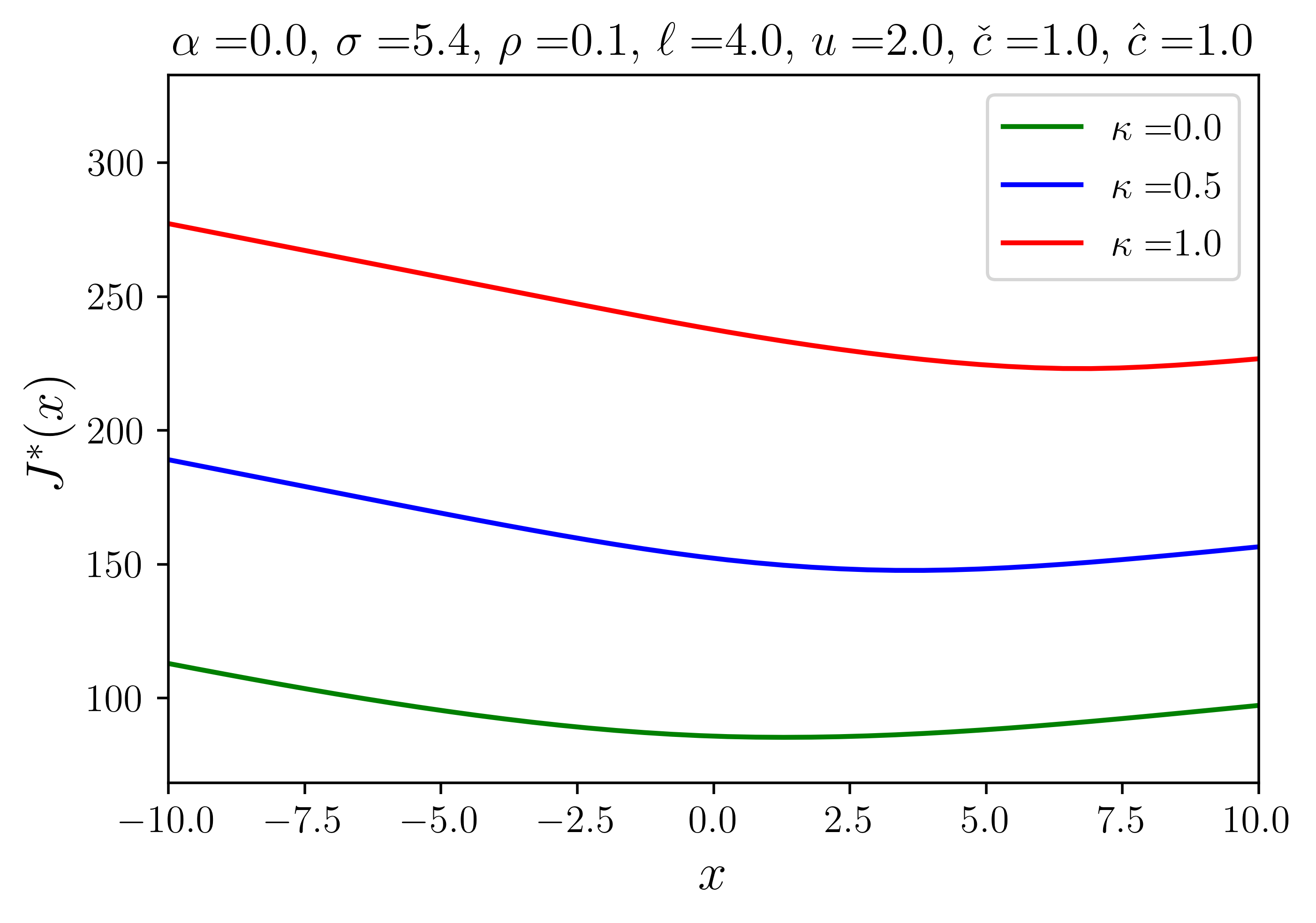
(a) varying $\kappa$ with $\sigma=5.4$

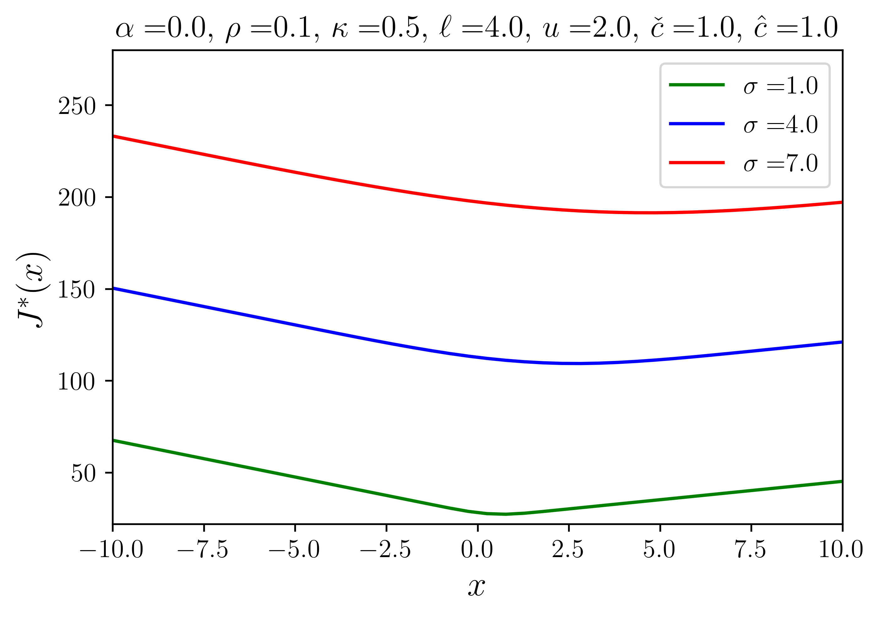
(b) varying $\sigma$ with $\kappa=0.5$

Figure 1: Cost functions for the parameter values $\rho=0.1$, $\alpha=0$, $\check{c}=\hat{c}=1$, $u=2$, and $\ell=4$.

Comparative statics of risk

As is common in the literature, we identify risk with the standard deviation of the cash process, $\sigma$, while we identify ambiguity with the set of density generators as parameterized by $\kappa$. First we explore the comparative statics of $\sigma$. As can be seen in Figure 2, the inaction region $({\underline{x}},xU)$ expands as $\sigma$ increases. That is, an increase in risk normally leads to a delay in taking action. However, note that in the symmetric case ($\alpha=0$), the inaction region expands less as $\kappa$ increases. This means that higher levels of ambiguity enforce earlier actions, which inevitably comes with higher costs. It highlights the pessimistic mindset of managers when they lack complete confidence in the drift of the cash flow process.

It is worth noting that these characteristics of risk and ambiguity not only persist in cases where the symmetry of the continuation region is violated, but also give rise to interesting features that are not commonly found in the standard literature on singular control. In the following numerical examples, we focus on the following asymmetries: (i) non-zero reference drift, (ii) inequality between the upper and lower control costs, and (iii) distinct holding costs for positive and negative cash balances.

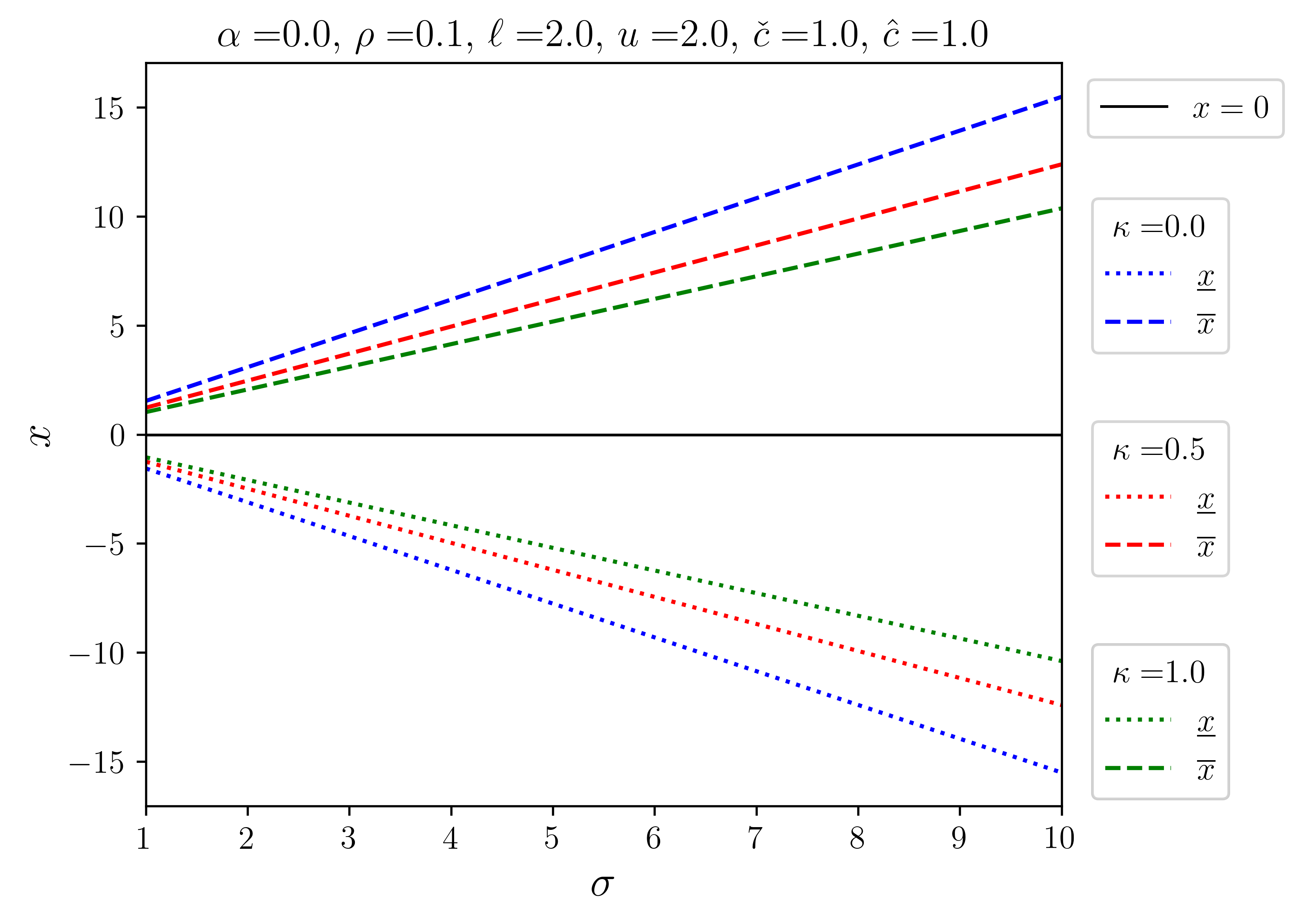
Figure 2: Control barriers for various $\kappa$ as a function of $\sigma$, with $\ell=u=2$, $\rho=0.1$, $\alpha=0$ and $\check{c}=\hat{c}=1$.

(a) increasing $\alpha$ with $\kappa=0$

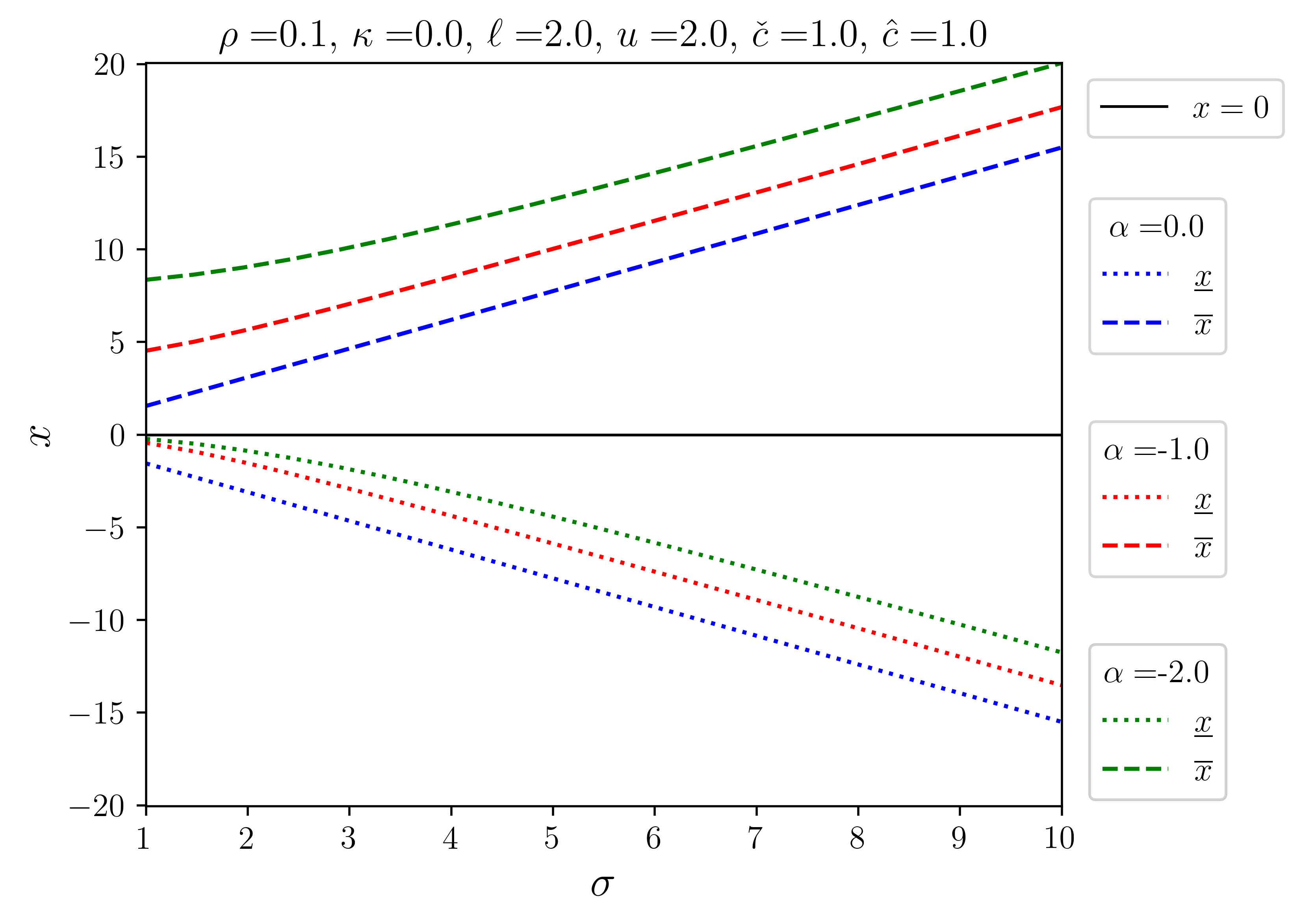
(b) decreasing $\alpha$ with $\kappa=0$

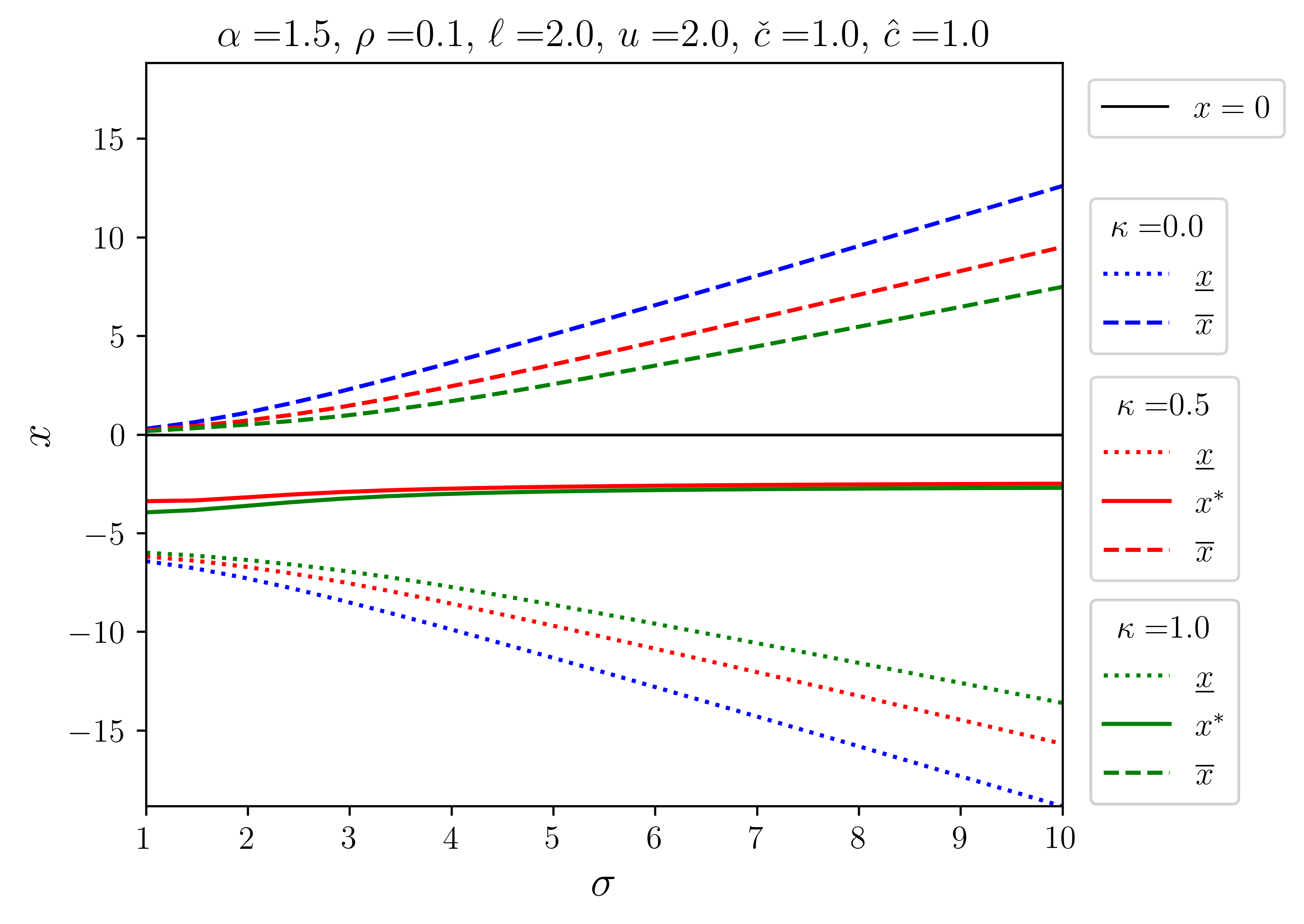
(c) increasing $\kappa$ with $\alpha>0$

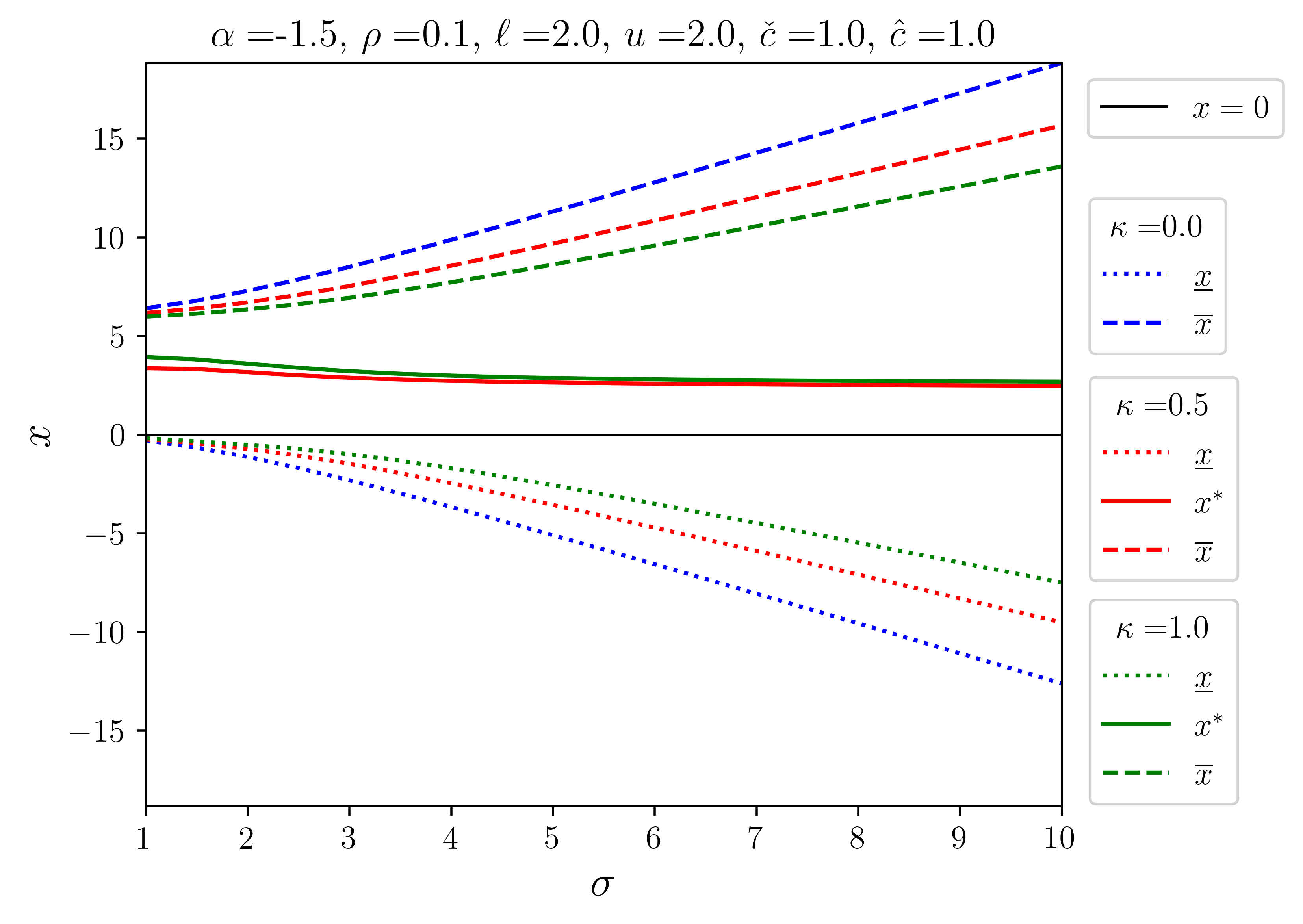
(d) increasing $\kappa$ with $\alpha<0$

Figure 3: Control barriers for varying $\alpha$ and $\kappa$ as a function of $\sigma$, with $\ell=u=2$, $\rho=0.1$, $\alpha=0$ and $\check{c}=\hat{c}=1$.

Comparative statics of drift

First, we look at the effect of changing the drift $\alpha$ under the reference prior. Figure 3(a) shows that for $\alpha>0$ the upper control barrier approaches the target level while the lower control barrier decreases. The inaction region undergoes a symmetric translation with an increase in $\alpha$. Conversely, Figure 3(b) shows the opposite effect when $\alpha<0$. This phenomenon can be intuitively understood as follows. The positive (negative) drift tends to increase (decrease) the cash level, on average, faster. This leads to an increase in the holding cost for positive (negative) cash balances. As a result, it becomes more (less) attractive to exert control for positive cash hoards and less (more) attractive to exert control for negative cash hoards.

To examine the impact of ambiguity on the control barriers, we select values of $\alpha$ from the set $\{-1.5,1.5\}$ and compare the results for different levels of $\kappa$ from the set $\{0.0,0.5,1.0\}$. For the case of $\alpha=1.5$, we observe that as the ambiguity level increases, the inaction regions shrinks as expected. Also note that the point where the worst-case drift changes, $x^{\ast}$, shifts downwards, which shows that ambiguity amplifies the positive drift; see Figure 3(c). A similar effect is observed in the opposite direction for $\alpha=-1.5$; see Figure 3(d). These findings suggest that a manager facing ambiguity should anticipate keeping their cash balance in the upper (lower) region for a longer time, incurring higher costs due to an increased likelihood of exercising the upper (lower) control. Meanwhile, the probability of having their cash hoard in the lower (higher) region decreases, resulting in, on average, a less expensive intervention.

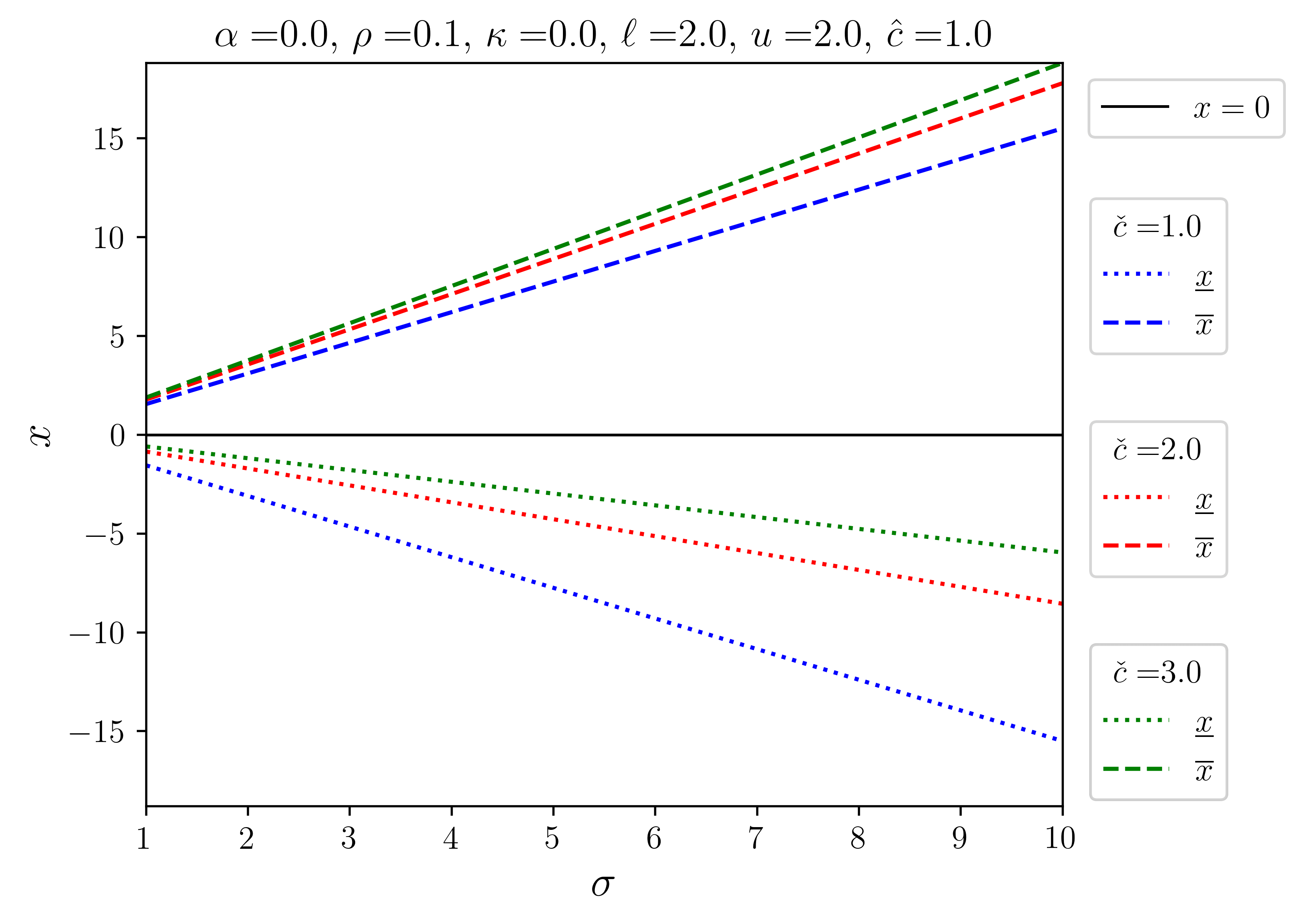
(a) increasing $\check{c}$ with fixed $\hat{c}$ and $\kappa=0$

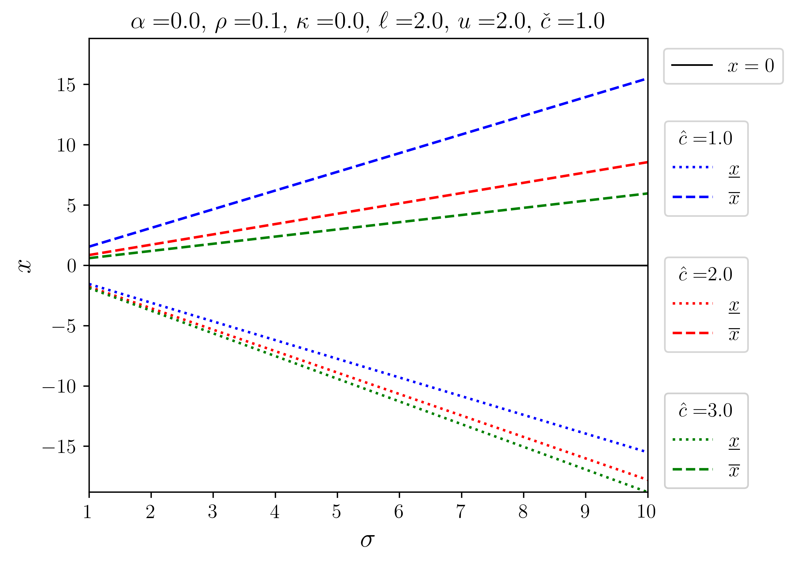
(b) increasing $\hat{c}$ with fixed $\check{c}$ and $\kappa=0$

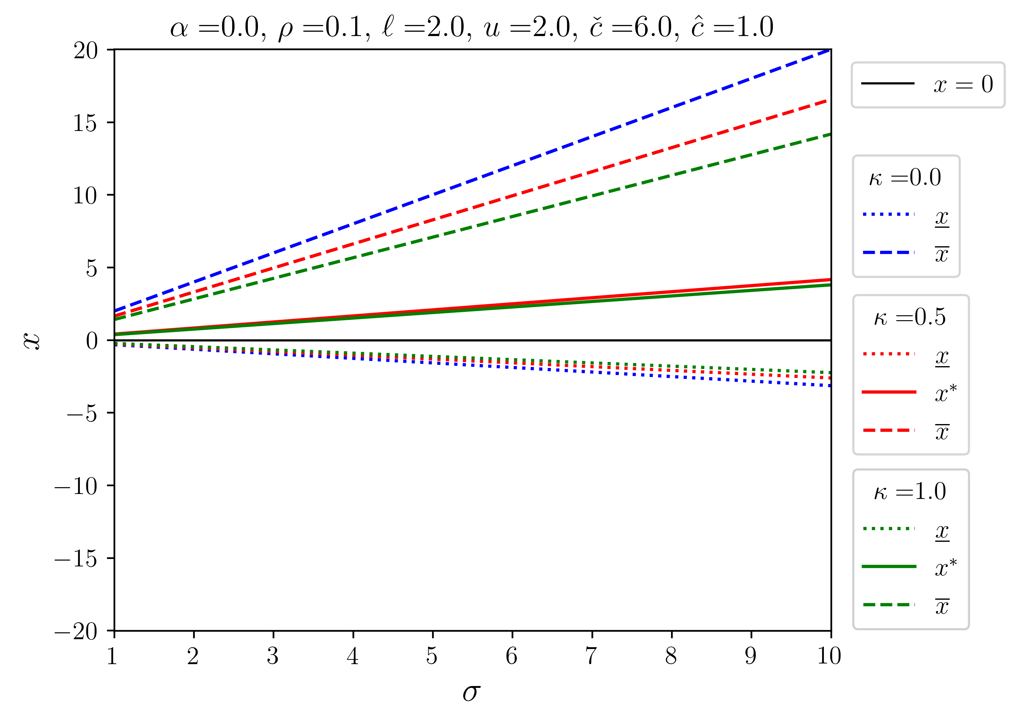
(c) increasing $\kappa$ with $\check{c}\geq\hat{c}$

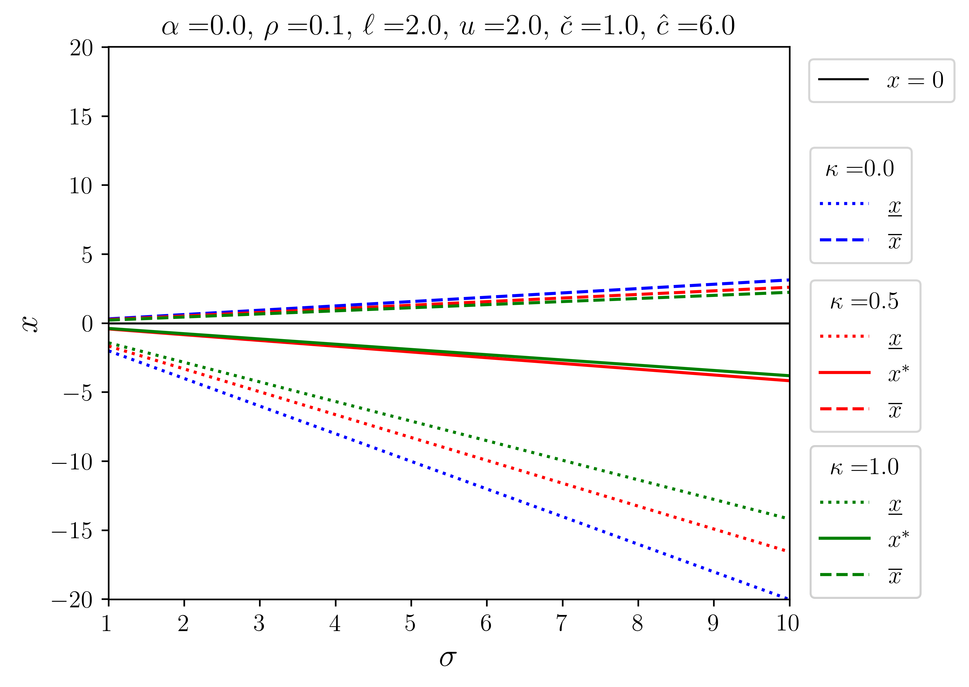
(d) increasing $\kappa$ with $\check{c}\leq\hat{c}$

Figure 4: Control barriers for varying $\hat{c}$, $\check{c}$ and $\kappa$ as a function of $\sigma$, with $\alpha=0$, $\rho=0.1$ and $u=\ell=2$.

Comparative statics of holding costs

We now consider the influence of the proportional holding costs of negative and positive cash balances on the control barriers. To examine this, we set $\check{c},\hat{c}\in\{1.0,2.0,3.0\}$ while all other parameters as in the base case. Figures 4(a) and 4(b) show that the difference between $\check{c}$ and $\hat{c}$ plays a role similar to that of the drift, $\alpha$, in determining the control barriers. Specifically, when $\hat{c}$ is greater (lower) than $\check{c}$, the inaction region rotates in a clockwise (counter-clockwise) direction. This phenomenon can be explained by two factors. Firstly, the optimal control policy leads to the upper (lower) barrier moving closer to the target level when $\check{c}<(>)\hat{c}$. This prompts the DM to exercise control sooner in order to prevent an increase in the holding cost. Simultaneously, it decreases (increases) the lower (upper) barrier, allowing the cash hoard to remain longer in the lower (upper) inaction region and thereby reducing the cost of holding cash. Secondly, when $\check{c}<(>)\hat{c}$ the cost function becomes more (less) convex where the cost function is increasing (decreasing). This creates an asymmetry between positive and negative cash balances and contrasts with the previous scenario where the “upper” and “lower” inaction regions were equivalent. These two factors together contribute to the observed rotation of the inaction region.

When we fix $\check{c}-\hat{c}$ and increase levels of ambiguity, we observe an amplification of the familiar “shrinking” of the control barriers, as depicted in the lower panel of Figure 4. An interesting interplay arises between the optimal control policy and maxmin utility. As $\kappa$ increases, the inaction region with a narrower width (corresponding to a higher instantaneous holding cost) shrinks even further, leading to a counter-intuitive effect of ambiguity. Since the previous result implies that it is costlier to remain in a narrower inaction region, the additional shrinkage induced by the optimal control policy encourages the cash balance to stay in the other region for a longer duration to mitigate against the holding cost. This represents a trade-off between maxmin utility and the optimal control policy. Importantly, the optimal control policy not only determines the control barriers but also influences the point at which the worst-case scenario changes.

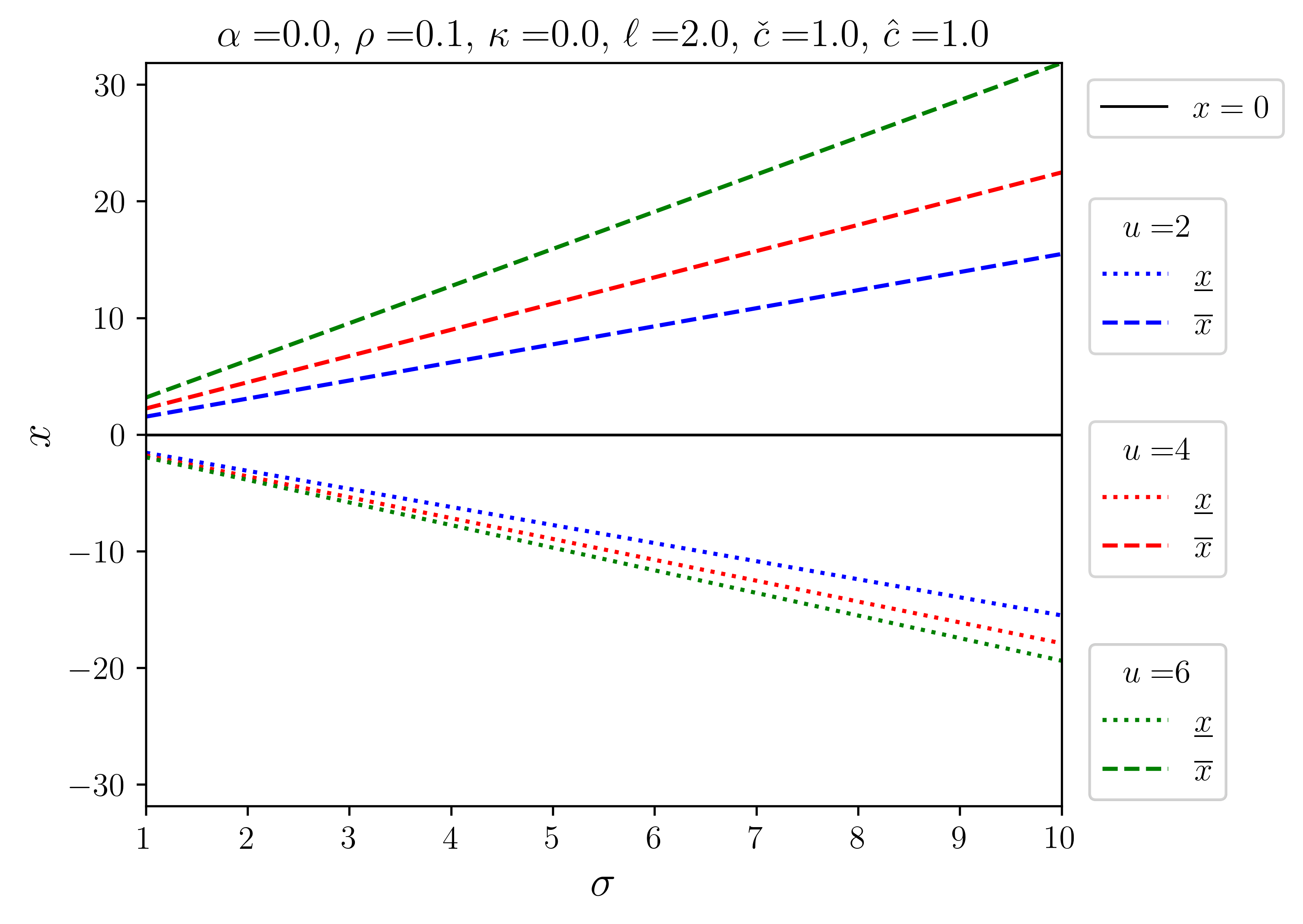
(a) increasing $u$ with fixed $\ell$ and $\kappa=0$

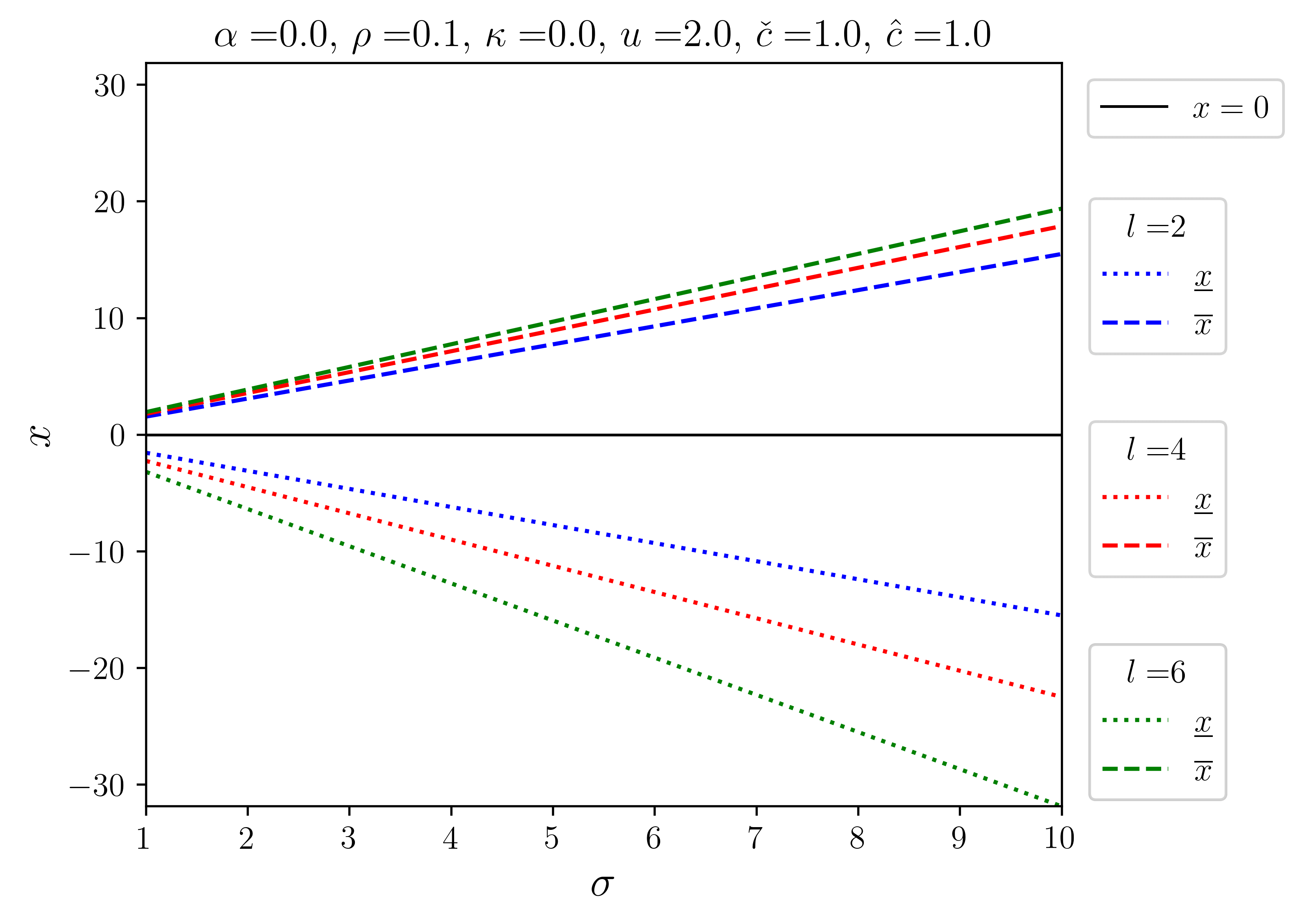
(b) increasing $\ell$ with fixed $u$ and $\kappa=0$

(c) increasing $\kappa$ with $u\geq\ell$

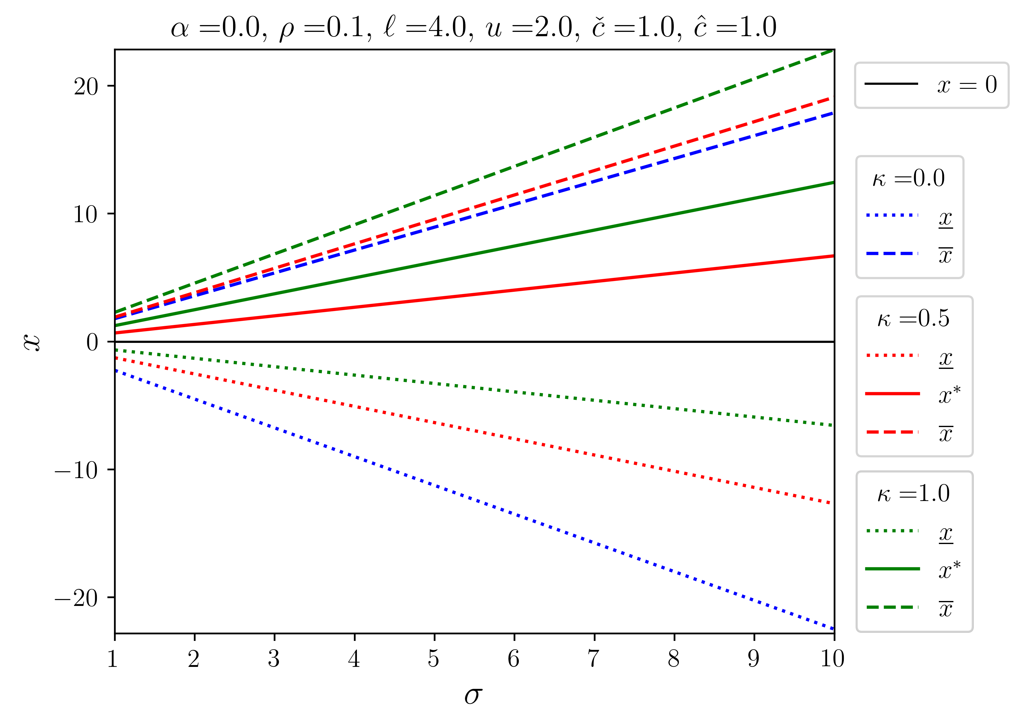
(d) increasing $\kappa$ with $u\leq\ell$

Figure 5: Control barriers for varying $u$, $\ell$ and $\kappa$ as a function of $\sigma$, with $\alpha=0$, $\rho=0.1$ and $\check{c}=\hat{c}=1$.

Comparative statics of control costs

We now examine the shape of control bands when there is an asymmetry in the instantaneous cost of control, i.e., when $\ell\neq u$. As previously, all other parameters are taken as in the base case. When examining the impact of the difference between $\ell$ and $u$ on control barriers, we observe in the upper panel of Figure 5 that increasing either value expands the entire inaction region. This expansion not only pushes the corresponding control barrier further away from the target level but also affects the other barrier. The reason behind this is clear: when $\ell<(>)u$, the cost of exercising the upper (lower) control becomes higher, prompting the manager to hold cash for a longer period rather than exercising control to minimize long-term cash holding costs. As the cost of controlling the cash balance at the opposite barrier decreases, the optimal control policy deviates from this barrier towards the target value, reducing the likelihood of the sample path reaching the more expensive side. This asymmetry is manifested in the shape of the value functions, which become more convex as the interval increases (decreases) when $\ell<(>)u$.

As $\kappa$ increases, all the previously mentioned characteristics persist, including the familiar shrinking effect illustrated in the lower panel of Figure 5. Additionally, there is a rotation of the inaction region, which represents another consequence of ambiguity and its interaction with the optimal control policy. Since it is more costly to exercise the upper (lower) control, an ambiguous manager anticipates that when the cash reserve is within the upper (lower) inaction region, it is more likely to approach the upper (lower) barrier, leading to even more expensive interventions in the long run. However, under the optimal control policy, the lower (upper) control barriers rotate in the same direction, enabling the manager to keep the cash balance in this region for a longer time, thereby mitigating the impact of ambiguity.

Comparative statics of ambiguity

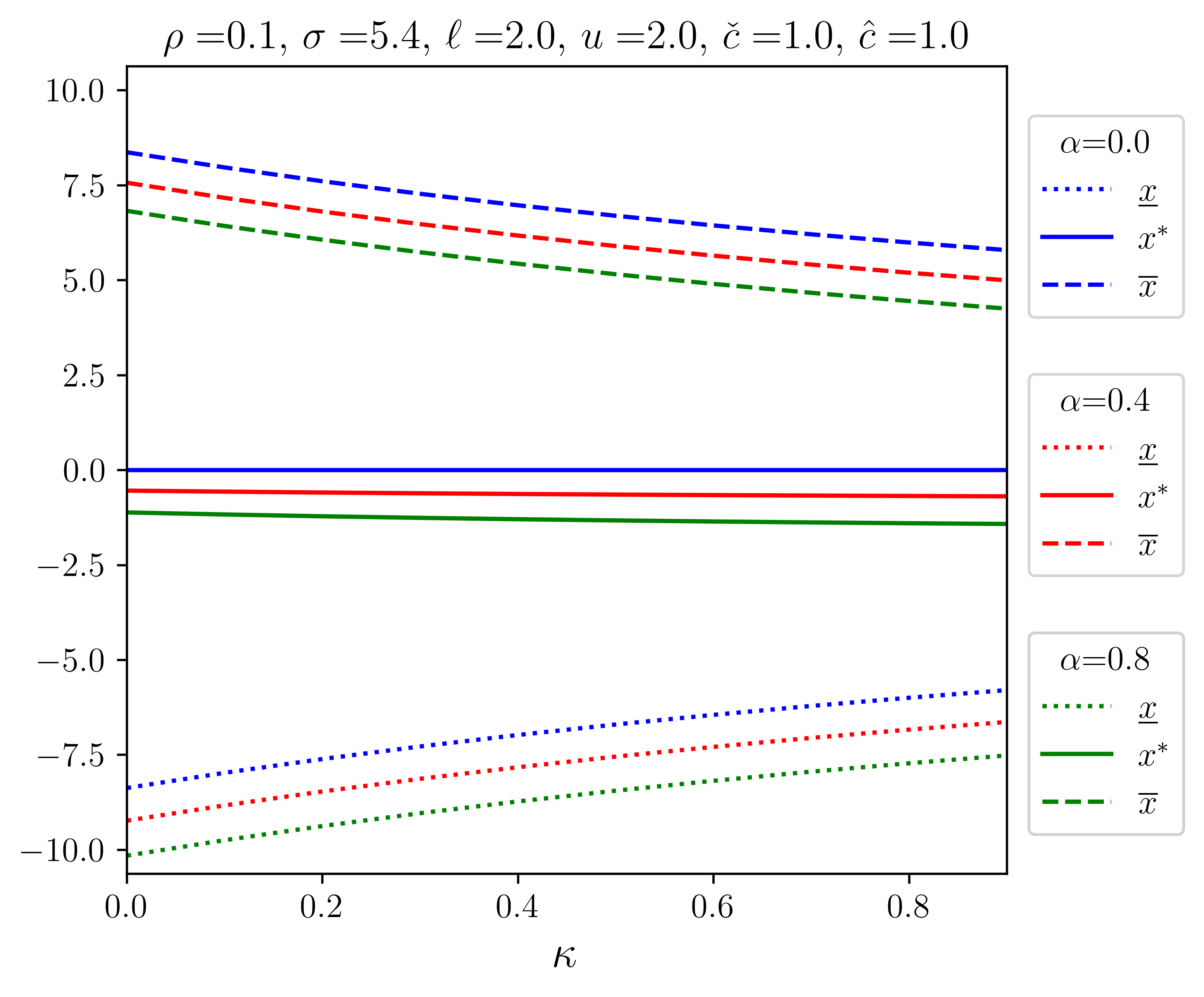
Figure 6: Control barriers with varying $\alpha$ as a function of $\kappa$.

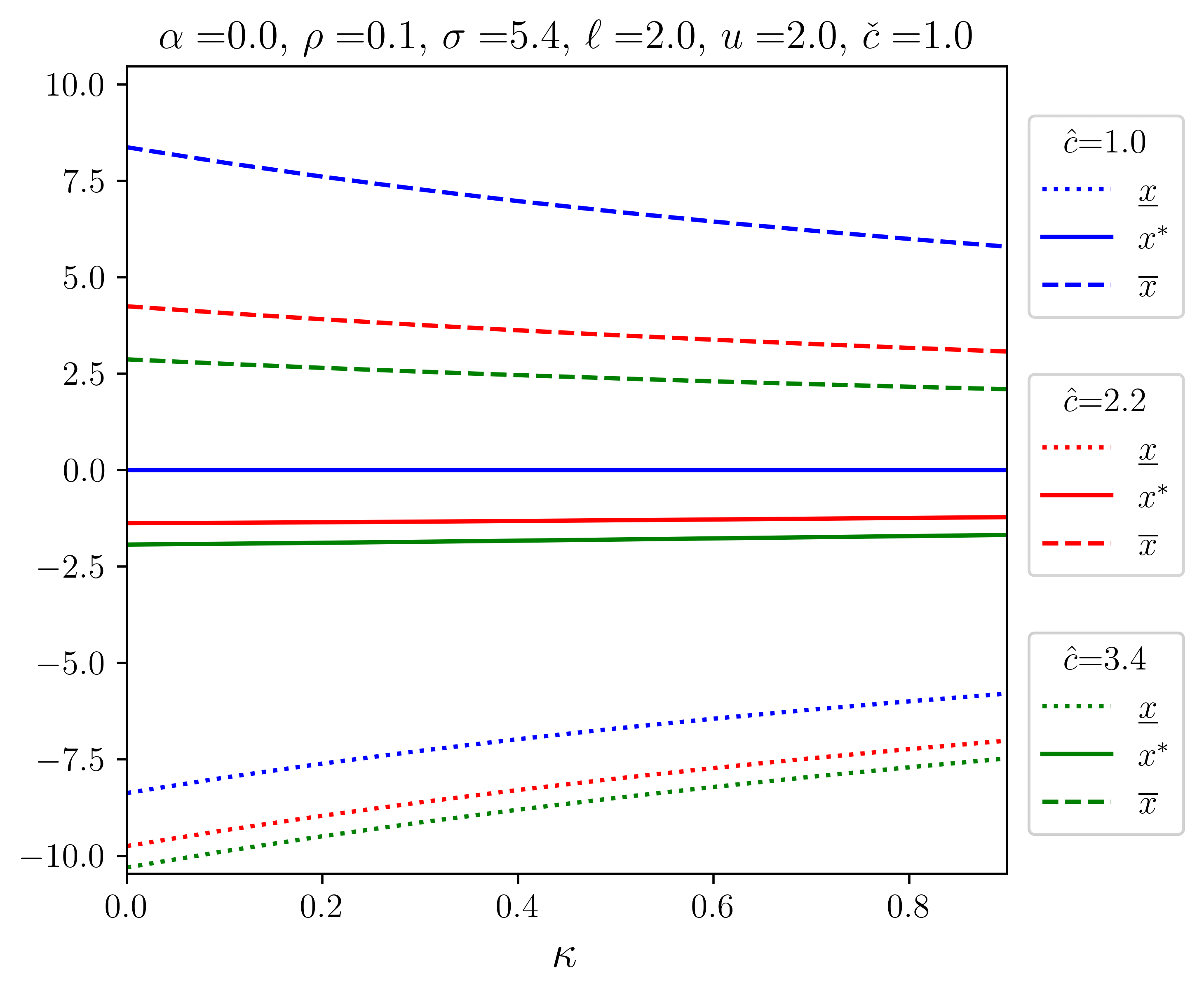
Figure 7: Control barriers with varying $\hat{c}$ as a function of $\kappa$.

Finally, we turn attention to the comparative statics of ambiguity, as measured by the parameter $\kappa$. As usual, we take the other parameters as in the base case. As we have seen throughout, the control barriers move closer to the target as $\kappa$ increases. That is, ambiguity accelerates control. We find that this effect holds both when the we vary $\alpha$ or $\check{c}-\hat{c}$. The effect is non-monotonic when control costs $\ell$ and $u$ are varied, because there is a point beyond which ambiguity delays control.

To illustrate these effects, let us first consider the typical cases when all parameters are fixed except $\alpha$ and $\check{c}-\hat{c}$. As we can see from Figures 6 and 7, the control barriers shrink as $\kappa$ increases. We also see the familiar downward translation when $\alpha$ and $\hat{c}$ increase (with fixed $\check{c}$). This is because increasing $\alpha$ elevates the upward drift of the controlled process (under the reference prior). A higher value of $\hat{c}$ leads to higher holding costs of positive cash balances, so that optimal control policy responds by translating the control barriers downward to minimise the cost function.

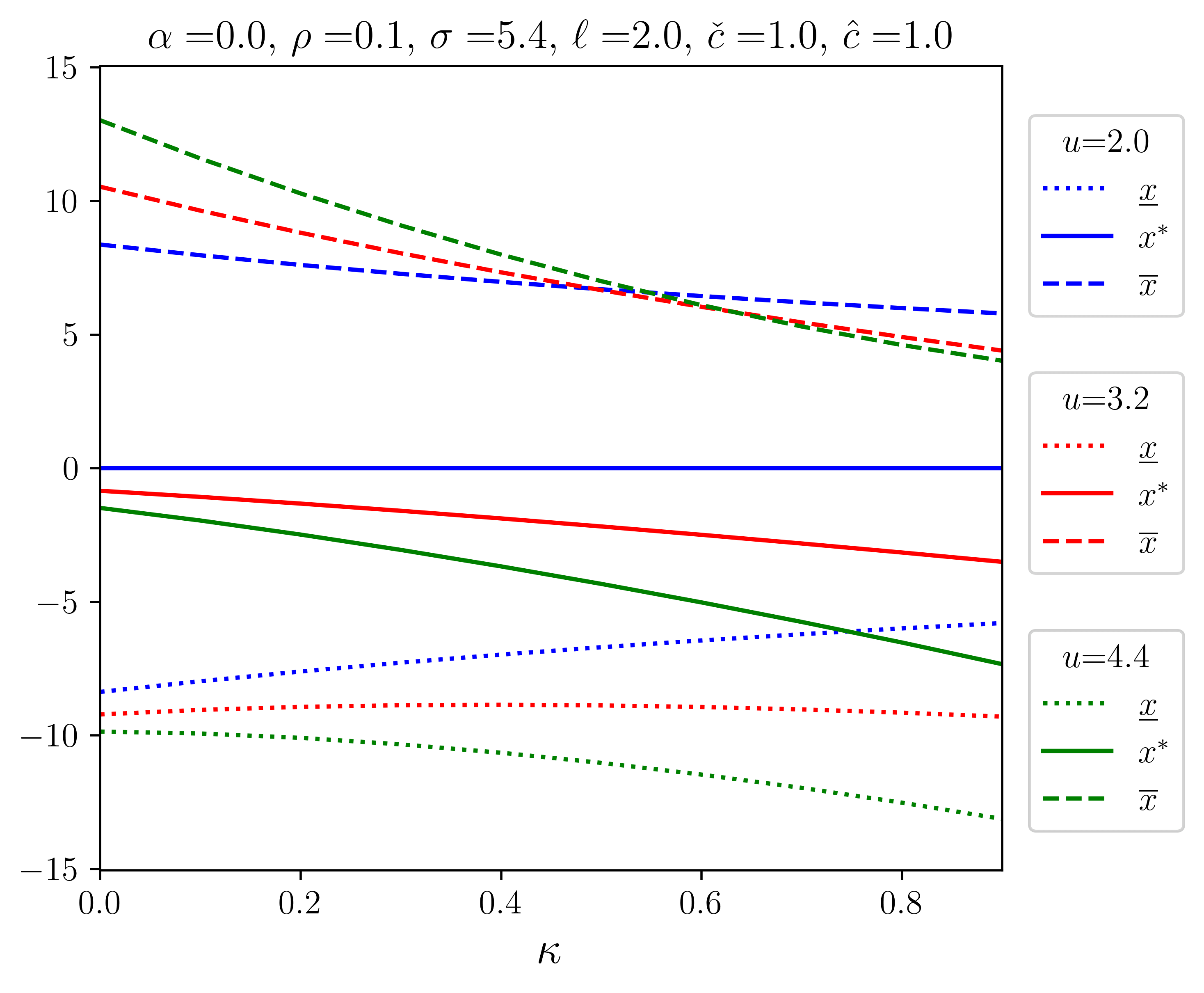
Figure 8: Control barriers with varying $u$ as a function of $\kappa$.

This effect no longer holds when considering variations in the control costs. Revisiting the results from the previous subsection, when $u>\ell$ and $\kappa$, the cost of exercising the upper control becomes relatively higher. Consequently, the optimal control policy is to delay control at the upper barrier. To achieve this, control at the lower control barrier is also postponed in an effort to keep the controlled process away from the upper control region. However, this relationship no longer holds in the presence of ambiguity. As shown in Figure 8, there exists a region where control of positive cash balances is activated earlier than without ambiguity. Furthermore, while an increase in ambiguity brings the upper barrier closer to the target level as expected, there is also a downward move of the lower control barrier. So, an ambiguity-averse manager is willing to pay a higher cost, because a higher level of ambiguity encourages more frequent exercise of the more expensive control. Meanwhile, the optimal control policy appears to mitigate against this extra cost by adjusting the lower barrier downward, with the resulting expectation that the controlled process will spend more time in the lower inaction. This effect reduces the overall expected discounted cost of cash holdings. These opposing effects result in an unconventional shape of the control barriers, which not only amplifies the impact of ambiguity but also highlights the interplay between ambiguity and the optimal control policy.

6 Conclusion

In this paper, we revisit the classical problem of two-sided singular control in the optimal cash reserve problem where the net cash position evolves according to an Itō diffusion. We extend this model to allow for managerial ambiguity use the maxmin expected utility framework $\kappa$-ignorance. We establish a verification theorem and use a numerical example to explore the effects of ambiguity on the optimal control of cash holdings.

From a managerial perspective, the most important observation we make is that ambiguity increases the frequency with which control is exerted. This is due to the fact that under the worst-case prior the manager expects higher holding costs, which makes exerting control relatively cheaper. This results, on average, in a smaller cash inventory, which is the opposite effect to an increase in risk. If risk, as measured by the variance of the random walk that affects the net cash flow, increases then the standard “option value of waiting” (cf., Dixit and Pindyck,, 1994) increases which implies that, typically, control is exerted later. This results in a larger cash inventory, on average.

There are several avenenues for future research. First, one of the assumptions of our model is that the manager does not learn. It is as if the manager is confronted with a new Ellsberg urn at every point in time. In many real-world situations it may be more realistic to assume that the manager is confronted with the same Ellsberg urn at every point in time. This then opens up the possibility of managerial learning. Secondly, our model of $\kappa$-ambiguity describes a fairly extreme version of cautious behavior. A more realistic version of the model would allow the manager to average over multiple priors. That would naturally lead to the smooth ambiguity model of Klibanoff et al., (2005).

References

Alvarez, (2003)
Alvarez, L. (2003).
On the properties of -excessive mappings for a class of
diffusions.
Annals of Applied Probability, 13:1517–1533.
Bather, (1966)
Bather, J. A. (1966).
A continuous time inventory model.
J. Appl. Probab., 3(2):538–549.
Baumol, (1952)
Baumol, W. J. (1952).
The transactions demand for cash: An inventory theoretic approach.
Q. J. Econ., 66(4):545–556.
Chakraborty et al., (2021)
Chakraborty, P., Cohen, A., and Young, V. R. (2021).
Optimal dividends under model uncertainty.
arXiv preprint arXiv:2109.09137.
Chen and Epstein, (2002)
Chen, Z. and Epstein, L. (2002).
Ambiguity, risk, and asset returns in continuous time.
Econometrica, 70(4):1403–1443.
Cheng and Riedel, (2013)
Cheng, X. and Riedel, F. (2013).
Optimal stopping under ambiguity in continuous time.
Math. Financ. Econ., 7(1):29–68.
Constantinides, (1976)
Constantinides, G. M. (1976).
Stochastic cash management with fixed and proportional transaction
costs.
Manage. Sci., 22(12):1320–1331.
Deshmukh et al., (2021)
Deshmukh, S., Goel, A., and Howe, K. (2021).
Do CEO beliefs affect corporate cash holdings?
Journal of Corporate Finance, 67:101886.
Dixit and Pindyck, (1994)
Dixit, A. K. and Pindyck, R. S. (1994).
Investment under uncertainty.
Princeton Univ. Press, Princeton, NJ.
Ellsberg, (1961)
Ellsberg, D. (1961).
Risk, ambiguity, and the savage axioms.
The Quarterly Journal of Economics, 75:643–669.
Eppen and Fama, (1969)
Eppen, G. D. and Fama, E. F. (1969).
Cash balance and simple dynamic portfolio problems with proportional
costs.
Int. Econ. Rev., 10(2):119–133.
Epstein and Ji, (2013)
Epstein, L. G. and Ji, S. (2013).
Ambiguous volatility and asset pricing in continuous time.
Rev. Financ. Stud., 26(7):1740–1786.
Epstein and Wang, (1994)
Epstein, L. G. and Wang, T. (1994).
Intertemporal asset pricing under knightian uncertainty.
Econometrica, 62(2):283–322.
Ferrari et al., (2022)
Ferrari, G., Li, H., and Riedel, F. (2022).
A knightian irreversible investment problem.
J. Math. Anal. Appl., 507(1):125744.
Fouque et al., (2016)
Fouque, J.-P., Pun, C. S., and Wong, H. Y. (2016).
Portfolio optimization with ambiguous correlation and stochastic
volatilities.
SIAM Journal on Control and Optimization, 54(5):2309–2338.
Gilboa and Schmeidler, (1989)
Gilboa, I. and Schmeidler, D. (1989).
Maxmin expected utility with non-unique prior.
Journal of Mathematical Economics, 18(2):141–153.
Hansen and Miao, (2018)
Hansen, L. P. and Miao, J. (2018).
Aversion to ambiguity and model misspecification in dynamic
stochastic environments.
Proc. Natl. Acad. Sci. U. S. A., 115(37):9163–9168.
Hansen and Miao, (2022)
Hansen, L. P. and Miao, J. (2022).
Asset pricing under smooth ambiguity in continuous time.
Econom. Theory, 74(2):335–371.
Hansen and Sargent, (2010)
Hansen, L. P. and Sargent, T. J. (2010).
Fragile beliefs and the price of uncertainty.
Quant. Econom., 1(1):129–162.
Hansen and Sargent, (2011)
Hansen, L. P. and Sargent, T. J. (2011).
Robustness and ambiguity in continuous time.
J. Econ. Theory, 146(3):1195–1223.
Hansen et al., (2006)
Hansen, L. P., Sargent, T. J., Turmuhambetova, G., and Williams, N. (2006).
Robust control and model misspecification.
J. Econ. Theory, 128(1):45–90.
Harrison and Taksar, (1978)
Harrison, J. and Taksar, M. (1978).
Instantaneous control of Brownian motion.
Mathematics of Operations Research, 8:439–453.
Harrison, (1978)
Harrison, M. (1978).
Optimal control of brownian storage system.
Stochastic Processes and Their Applications, 6:179–194.
Harrison, (2013)
Harrison, M. J. (2013).
Brownian Models of Performance and Control.
Cambridge University Press.
Harrison and Taksar, (1983)
Harrison, M. J. and Taksar, M. I. (1983).
Instantaneous control of brownian motion.
Hellmann and Thijssen, (2018)
Hellmann, T. and Thijssen, J. J. J. (2018).
Fear of the market or fear of the competitor? ambiguity in a real
options game.
Oper. Res., 66(6):1744–1759.
Jeanblanc-Picqué and Shiryaev, (1995)
Jeanblanc-Picqué, M. and Shiryaev, A. N. (1995).
Optimization of the flow of dividends.
Russian Mathematical Surveys, 50(2):257–277.
Jin and Yu Zhou, (2015)
Jin, H. and Yu Zhou, X. (2015).
Continuous-time portfolio selection under ambiguity.
Math. Control Relat. Fields, 5(3):475–488.
Karatzas and Shreve, (1991)
Karatzas, I. and Shreve, S. (1991).
Brownian motion and stochastic calculus, volume 113.
Springer Science & Business Media.
Klibanoff et al., (2005)
Klibanoff, P., Marinacci, M., and Mukerji, S. (2005).
A smooth model of decision making under ambiguity.
Econometrica, 73(6):1849–1892.
Knight, (1921)
Knight, F. H. (1921).
Risk, uncertainty and profit, volume 31.
Houghton Mifflin.
Lin and Riedel, (2014)
Lin, Q. and Riedel, F. (2014).
Optimal consumption and portfolio choice with ambiguity.
arXiv preprint arXiv:1401.1639.
Lin and Riedel, (2021)
Lin, Q. and Riedel, F. (2021).
Optimal consumption and portfolio choice with ambiguous interest
rates and volatility.
Econom. Theory, 71(3):1189–1202.
Nishimura and Ozaki, (2007)
Nishimura, K. G. and Ozaki, H. (2007).
Irreversible investment and knightian uncertainty.
J. Econ. Theory, 136(1):668–694.
Sarkar, (2000)
Sarkar, S. (2000).
On the investment–uncertainty relationship in a real options model.
Journal of Economic Dynamics and Control, 24:219–225.
Tanaka, (1979)
Tanaka, H. (1979).
Stochastic differential equations with reflecting.
Stochastic Processes: Selected Papers of Hiroshi Tanaka, 9:157.
Thijssen, (2011)
Thijssen, J. J. J. (2011).
Incomplete markets, ambiguity, and irreversible investment.
J. Econ. Dyn. Control, 35(6):909–921.
Tobin, (1956)
Tobin, J. (1956).
The Interest-Elasticity of transactions demand for cash.
Rev. Econ. Stat., 38(3):241–247.
Trojanowska and Kort, (2010)
Trojanowska, M. and Kort, P. M. (2010).
The worst case for real options.
J. Optim. Theory Appl., 146(3):709–734.
Vial, (1972)
Vial, J.-P. (1972).
A continuous time model for the cash balance problem.
LIDAM Reprints CORE.