Inferring Capabilities from Task Performance with Bayesian Triangulation

Abstract

As machine learning models become more general, we need to characterise them in richer, more meaningful ways. We describe a method to infer the cognitive profile of a system from diverse experimental data. To do so, we introduce measurement layouts that model how task-instance features interact with system capabilities to affect performance. These features must be triangulated in complex ways to be able to infer capabilities from non-populational data – a challenge for traditional psychometric and inferential tools. Using the Bayesian probabilistic programming library PyMC, we infer different cognitive profiles for agents in two scenarios: 68 actual contestants in the AnimalAI Olympics and 30 synthetic agents for O-PIAAGETS, an object permanence battery. We showcase the potential for capability-oriented evaluation.

1 Introduction

What does success or failure tell us about a system’s capabilities? In isolation, performance results are hard to interpret: most interesting tasks require several different abilities to be successfully combined. instances. For example, an agent exploring a 3D environment to find a reward needs to understand that the reward still exists when occluded (object permanence). It must then remember where it is, and successfully navigate to it. If the agent fails, we cannot know the cause: lack of object permanence, limited memory or navigation skills. This leads to poor predictability about the performance of the agent for new tasks, in or out of the training distribution.

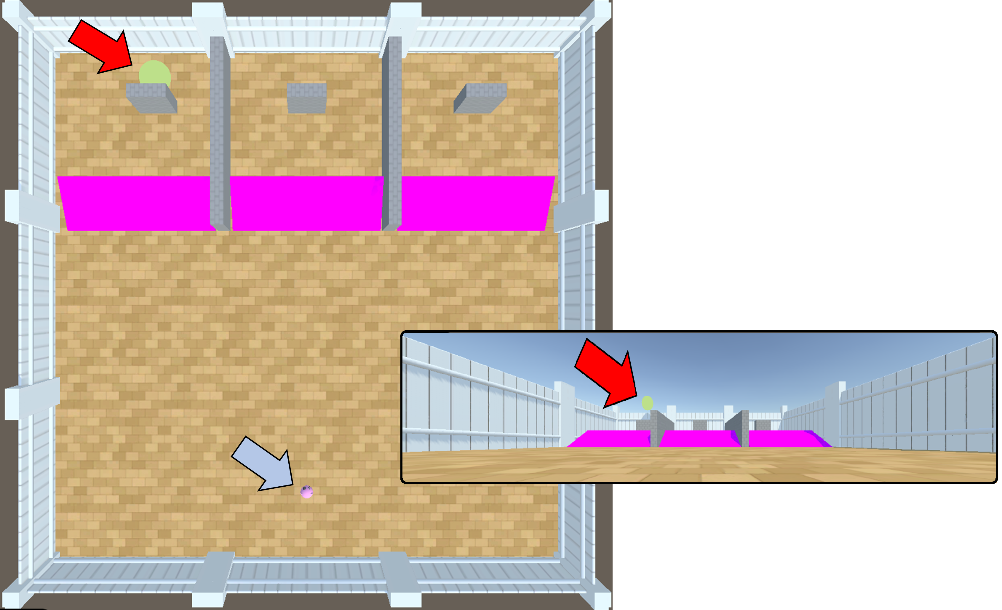
Figure 1: This task instance requires the agent to: (a) understand that the reward still exists when occluded (object permanence), (b) remember which of the three walls it is occluded behind while it navigates towards it (memory), and (c) reach it over ramps and around the wall (navigation).

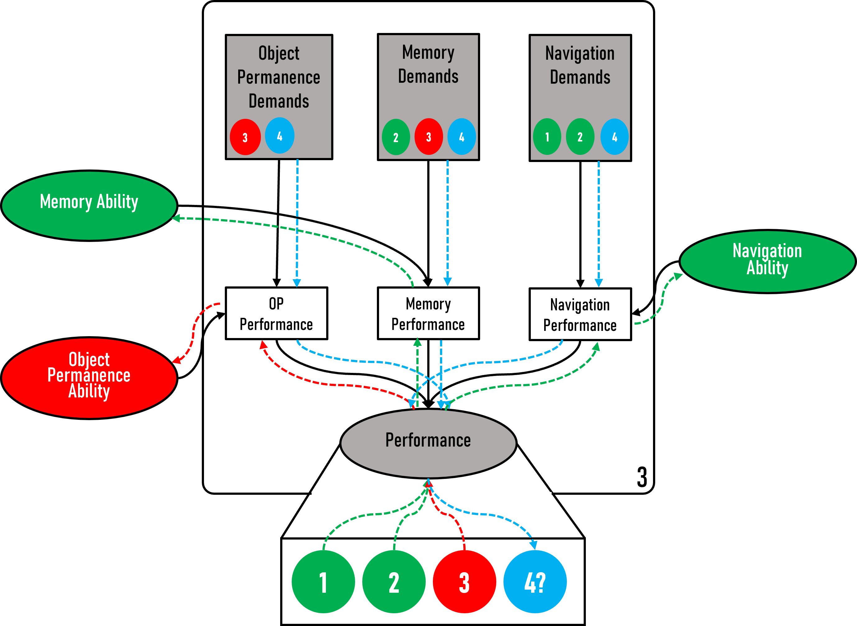
Figure 2: Triangulation in the measurement layouts using results from task instances like this one. Bottom-up inference from three tasks (in green and red for success and failure respectively) leading to the cognitive profile. Top-down inference (in blue) predicting failure for the fourth task.

However, suppose we also knew that the agent performs well on tasks that involve complex navigation, and the same for tasks involving memory. We could now infer that the system’s failure is likely a failure of object permanence by triangulation, a robust inferential method in formal epistemology (Heesen, Bright, and Zucker 2019) and causal (Bayesian) reasoning.

This bottom-up inference is illustrated in green and red in Fig. 2. We can use this information to draw conclusions about where the system is safe to deploy, and to direct efforts to improve it. We can also predict behaviour in new scenarios: for example, the agent will likely fail at a new task with high object permanence demands, as illustrated in blue in Fig. 2.

This example demonstrates that we can leverage the fact that different tasks—and their constituent instances—have different demands to help us extract conclusions about system capabilities from patterns of task performance. However, these conclusions require an analytical approach that facilitates complex inferences. If we were to examine each task or instance in isolation or to simply aggregate performance across all tasks, this triangulation of abilities would not be possible. To address this, we propose a novel Bayesian approach to evaluation that enables simultaneous inferences about multiple abilities from patterns of task performance. This approach has a series of principles facilitating a capability-oriented approach to the evaluation of machine learning models:

1. We do not simply break out performance by ‘categories’. Related work employs a ‘taxonomy of tasks’ (see e.g., Table 1 in (Liang et al. 2022)), each placed into one or more categories. This limits the inferential capacity and predictability of these category aggregates for new tasks. Instead, we evaluate based on instance demands.

2. Unlike psychometric approaches such as factor analysis (FA), structural equation modelling (SEM) or item response theory (IRT), we do not rely on populational data (Gustafsson and Undheim 1996). Instead, we infer the cognitive profile of a single subject from their performance data alone.

3. We do not ‘reify’ extracted latent variables as capabilities, which has been done hierarchically elsewhere, (e.g., the Cattell-Horn-Carroll model (Keith and Reynolds 2010)).

Instead, we identify general linking functions that help derive the requisite capabilities from the demands of the tasks.

4. Probabilistic models currently used in cognitive modelling (Lee 2011) are often simple at the level of the individual and cannot convey the required probabilistic expressions connecting individual performance, capabilities and task features. Instead, complex interactions allow for Bayesian triangulation which we use for informative evaluation. In this paper we find an operational solution to these inferential challenges in the form of Measurement Layouts: specialised and semantically-rich hierarchical Bayesian networks. Using the inference power of the No U-Turn Sampler (Hoffman and Gelman 2014) in PyMC (Salvatier, Wiecki, and Fonnesbeck 2016), a probabilistic programming engine, we can triangulate from performance and the task’s cognitive demands to the capability and bias levels for each subject (their cognitive profile). Then, performance can be inferred downstream for new tasks.

We derive the cognitive profiles in two scenarios: the contestants in the AnimalAI Olympics (Crosby et al. 2020) and several synthetic agents for O-PIAAGETS (Voudouris et al. 2022), an object permanence battery. We show how systems with similar overall performance can have very different capability levels and biases.

2 Background

AI systems are often evaluated on one or more standard benchmarks. Because of the remarkably broad capabilities of modern systems, benchmarks are becoming larger and more diverse. For instance, BIG-bench (Srivastava et al. 2022) contains over 200 tasks for evaluating language models. Aggregating many tasks into a single score does not allow for nuanced conclusions about where or why a system fails (Burnell et al. 2023), and has little value for predicting system performance a specific unseen task.

Analysing 200 tasks separately would lead to an unwieldy and hard to interpret set of results. One option is the categorisation of tasks across several dimensions, providing a moderate level of insight into where a model succeeds or fails (Osband et al. 2019; Ilievski et al. 2021; Crosby et al. 2020; Liang et al. 2022). However, conclusions are highly dependent on how instances are assigned to categories, and predictive value is limited inside and across categories.

An widely-used approach that does not require any taxonomy of capabilities is to extract and reify them from the data. Given experimental data for many tasks and subjects, we can use Factor Analysis (FA) to infer those factors that best explain the observed variance in the population. Some structure can be inferred from FA, as in the classical hierarchical models (Cattell-Horn-Carroll model (Keith and Reynolds 2010)), but today it is common to use more powerful techniques such as Structural Equation Modelling (SEM) (Ullman and Bentler 2012). However, SEM assumes linear relationships between variables and that dependent variables have normally distributed sample means. These assumptions are unlikely in the real world. Further, SEM is a populational technique requiring a large sample of individuals in order to confirm structural relationships.

A more granular approach is to identify the difficulty of each task instance and the ability of each system based on the relationship between task difficulty and the system’s performance. This idea is the cornerstone of Item Response Theory (IRT) (Embretson and Reise 2000; De Ayala 2009).

When several abilities exist, we must rely on multidimensional IRT(Reckase 2009) However, IRT is also populational, and derives abilities and difficulties relative to population averages, therefore the parameters of the same item can change if we add new items, or the abilities of a system may change if we add more systems. This poses a problem for AI evaluation, where the population of individual systems is constantly changing and advancing.

Still, with FA, SEM, IRT or other techniques, patterns of performance are mapped to capabilities, making up a multi-dimensional characterisation of the subject that is sometimes called a cognitive profile (Letteri 1980). Cognitive profiles make it possible to identify differences that might go unnoticed in aggregated scores, make predictions about future performance, and gain insights into the relationships between different abilities (e.g., deficits in mental rotation are one cause of poor spatial navigation).

Most psychological assessment is populational. Exceptions can mostly be found in developmental psychology and animal cognition (Moran et al. 2017; Bergman and Andersson 2015; Shaw and Schmelz 2017). The scarcity of subjects and the difficulty of experiments results in an emphasis on carefully designed tasks that ensure a systematic coverage of the relevant features and possible distractors. On the other hand, if the cognitive mechanisms for solving the task are accurate and enough variation is introduced, as in the example of Fig. 2, the results can be sufficient to estimate the capabilities of a single individual, independently of the other evaluated individuals. This is the type of approach that we need to evaluate ML models and AI systems.

Fortunately, there is recent movement towards producing training and test variations, augmented examples or corruptions to test systems, through adversarial learning (Zellers et al. 2018; Nie et al. 2019; Rozen et al. 2019; Kiela et al. 2021), procedural content generation (Risi and Togelius 2020) and other domain-specific techniques (Sugawara, Stenetorp, and Aizawa 2020). These variations have also been inspired by software testing, such as (Marijan and Gotlieb 2020) and (Ribeiro et al. 2020). Some of this effort results in annotated datasets, especially for reinforcement learning — from the inspiration behind the AnimalAI Olympics (Crosby et al. 2020) to the fully-systematic O-PIAAGETS (Voudouris et al. 2022). However, the next step of using these annotated data for capability-oriented evaluation has not been taken yet.

Not using populational data has to be compensated by a larger number of varied instances. When many dimensions of variation are introduced, the inference problem becomes complex. Traditional Bayesian Networks (BN) (Ben-Gal 2008) can be used for arbitrarily sophisticated probability distributions. For complex networks, though, performing the inference calculation is computationally intractable (Cooper 1990). Approximation techniques for Bayesian inference (BI) have been introduced, including the Markov Chain Monte Carlo family (Andrieu et al. 2003), allowing for the inference of latent values in more complex BNs, particularly those with multiple levels of dependency and complex relations between variables. Taking advantage of these recent advances in Bayesian approximation, evaluation procedures, and computing power allows us to extend the benefits of capability-oriented evaluation to machine learning for the first time, enabling more robust, thorough, and principled evaluations of ML systems.

3 Measurement Layouts

Performance can be understood as a function of task demands and capability levels. The precise relation between the two depends on the task features and the tested capabilities. For instance, in a memory problem, the number of objects to remember in a particular task demands a memory capability level at least as high as the number of objects. However, the difference between task demands and capability levels is likely not sufficient to account for all variance in observed performance. Cognitive biases, such as a preference or aversion to apparently irrelevant features like colour, can also affect performance. Finally, AI systems can exhibit a lack of robustness caused by some unaccounted factors or noise. Cognitive profiles need to include all of these. Let us define more precisely a task characterisation and the corresponding cognitive profile. We will then detail how they are connected by the measurement layouts.

Definition 3.1.

A task characterisation is a set of observable, usually constructed, meta-features $X$, expressing cognitive demands and other high-level properties of the task.

For instance, in an image classification problem, the level of blur of the image or the level of clutter of the background could constitute perceptual demands. Many other properties may also, in practice, affect performance.

Definition 3.2.

The cognitive profile of a system is a tuple $\langle C,B,R\rangle$. Where $C$, $B$, and $R$ are vectors of capability levels, bias, and robustness values respectively.

Capability levels represent what the system can do, bias values represent some other preferences or limitations that may impact performance in a less monotonic way, and robustness levels account for reliability issues, unexplained or random effects (noise) on either the agent or environment.

Definition 3.3.

A measurement layout is a directed acyclic graph that connects, through linking functions, the meta-features of a task characterisation with the cognitive profile of a system, in order to predict observed performance.

We define measurement layouts as Hierarchical Bayesian Networks (HBN) (Murphy 2023) with the following characteristics: Within the measurement layout we include a node for every meta-feature in every task instance and a node for each element of the system’s cognitive profile. All of them are roots of the graph. A connection $A\rightarrow B$ denotes that $B$ is conditionally dependent on $A$. Linking functions are used to formally define relationships between dependent nodes.

All nodes within the HBN define a probability distribution. We can classify nodes into three categories depending on the provenance of their summary statistics:

Metafeatures: These come from the task characterisation and are fixed, observable values. They are represented as a fixed Dirac-delta distribution.

Cognitive Profile Nodes: These are elements of the cognitive profile relevant to assessed task’s demands. This includes required capabilities and likely biasses. These often combine with meta-features and feed in to derived nodes. The range and distribution of these elements derives from the task characteristics. To make our inferences as data-driven as possible these begin with uninformative priors.

Derived Nodes: These are instance-level inferences. They are combinations of meta-features and/or cognitive profile elements that have their parameters derived from dependent nodes. Information to compute these values is encoded in the linking function for the node, the output of which is used as the summary statistics of the node’s distribution.

One derived node is the observable performance for the task—the only leaf node—but most are Intermediate Non-Observable Nodes (INON), which represent intermediate performances or effects. All three node types were seen in Fig. 2 (right). The connective structure can be enriched by domain knowledge determining which cognitive profile elements and meta-features are expected to affect the values of instance-level inference nodes. These relationships can be higher-order and complex, with certain INON nodes requiring the nuanced confluence of many cognitive profile elements and meta-features. Complex connective structure (and the requirement for increased levels of domain knowledge) can arise from the need to accurately distinguish between success, failure, and the multitude of confounding behaviour that a carefully designed benchmark must account for.

By a linking function, we refer to any mathematical expression that maps values from the outputs of one node’s probability distribution to the input of another.

For instance, it could be a sigmoid function of the difference between capabilities and demands. It could also be a product of (non-compensatory) capabilities, representing a quantitative and differentiable expression for a logical ‘and’. Alternatively, it could be some additive linear equation, representing a quantitative expression of a logical ‘or’, when some preceding nodes are compensatory—or a generalised mean in between. The functions can scale the incoming nodes, so that we adjust the ranges for capabilities, biases and noise. The possibilities are endless; in practice we use only a few kinds of linking functions. We give the specific equations for the linking functions that we used used in this work in Tables 3 and 5 in the appendix. These are used in the two scenarios that follow.

A key conceptual difference between our measurement layouts and typical use cases for HBNs is that our approach is trying to capture a hierarchical dependency relation on capabilities and demands, rather than encoding information on hyper-priors. The linking functions between nodes are often non-linear, conceived from domain knowledge of the task and applying ideas from cognitive modelling.

For instance, one of the key decisions is to determine when some capabilities are independent, and if so, whether they are compensatory or not, being realised with additive or multiplicative expressions respectively. If they are not independent, then an arrow has to connect them with a linking function expressing this dependency mathematically.

Given the cognitive profile of a system, and the characterisation of a new task, we can use the measurement layout to anticipate performance by forward (top-down) inference. But before that we need to infer the cognitive profile from the observed performance of other tasks by backward (bottom-up) Bayesian inference. For this, we utilise PyMC’s inference engine and the No U-Turn Sampler (Hoffman and Gelman 2014) approach to BI (see Appendix A for a detailed description). For this to accurately predict a system’s cognitive profile, the test battery

requires instances to jointly control for alternative explanations permitting performance results to ‘triangulate’ latent capabilities.

4 Cognitive Profiles for the AAI Olympics

To illustrate how a measurement layout identifies cognitive profiles, we first select a domain with simple task characterisations that can be straightforwardly related to cognitive profiles to predict performance.

The Animal-AI Olympics (AAIO) (Crosby et al. 2020) meets all these requirements. The AAIO was an open competition evaluating AI agents in a 3D environment, where agents had to get a reward by locating it and navigating in an arena.

Participants were asked to build systems (usually reinforcement learning agents) and train them on their own custom-built tasks in the AAI Environment. Screenshots for two tasks are shown in Fig. 7 located in Appendix B along with more information about AAIO and the environment. We select 69 tasks from the competition test set that evaluate simple goal-directed behaviour. We include 68 participant agents for which we know nothing about their design.

4.1 Measurement Layout

In this domain, following the analysis performed in (Burnell et al. 2022), the set of meta-features $X$ of the instances that characterise task instances are rewardSize, rewardDistance, Xpos and rewardBehind. These represent the reward’s size, distance, and if it is left, right, in front, or behind the agent.

The cognitive profile is composed of two capabilities, navigationAbility and visualAbility, respectively representing the skill to move around purposefully and the visual acuity of the agent, one bias rightLeftBias, representing any preference for left or right movements, and one robustness level noiseLevel, accounting for any unexplained variability.

We then compare the profile of the agent to the demands of the task to derive performance. This is our measurement layout, as can be seen in Fig. 4 (left). The metafeatures $X$ appear as observed (shaded) nodes in the model, appearing within the plate, with 69 instances. The elements of the cognitive profile appear as external latent (unshaded) variables.

The derived nodes lie at the intersection of the meta-features and the external cognitive profile nodes.

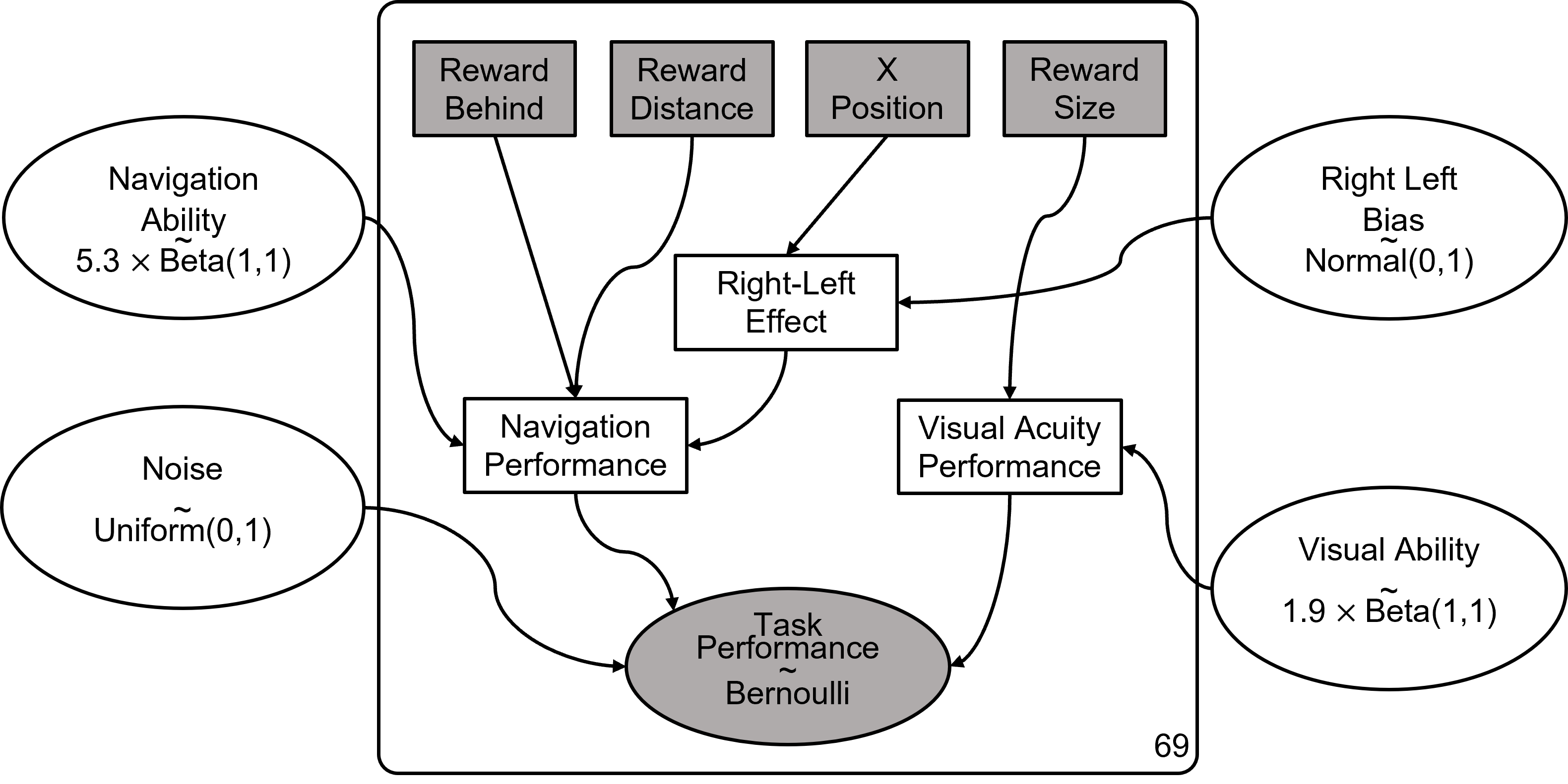
Figure 3: Measurement layout for the Animal AI Olympics.

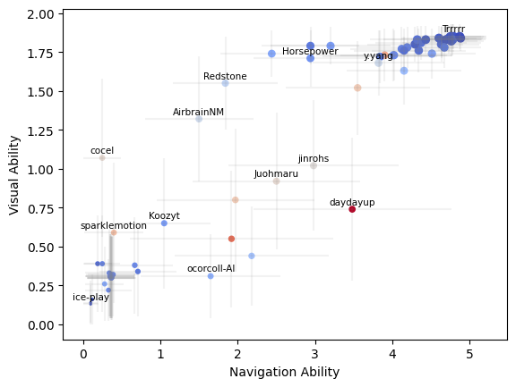
Figure 4: Cognitive profiles of the 68 agents in AAIO, with names shown for some of them. The $x$-axis and $y$-axis show the inferred means for navigationAbility and visualAbility respectively, with their standard deviations as error bars in grey. The radius of each point represents the average performance, while the colour represents the noiseLevel, with red representing higher noise than blue.

Not visible in the figure are the linking functions associated with each arrow. The variable rightLeftEffect is calculated as the product between rightLeftBias and XPos, since left/right bias and XPos are represented with negative and positive values respectively, so the product gives a positive result when both go in the same direction. This rightLeftEffect, jointly with rewardBehind and rewardDistance affect navigationPerformance, a non-observable intermediate performance variable. The exact formulation of how these three variables are integrated can be found in Appendix C.2,

but broadly the linking function subtracts the effects of reward distance and position relative to the agent’s viewpoint (e.g., behind) from the navigation ability and adds the right-left bias to this. The linking function then applies a logistic function to this margin to give a value between 0 and 1 for navigationPerformance. The process to derive visualPerformance is similar, simply subtracting rewardSize ( inverted so the higher the smaller) from visualAbility.

Note that the ranges of these two abilities are given by the ranges of the task metafeatures, with navigationAbility in $[0,5.3]$ and with visualAbility in $[0,1.9]$ respectively, representing how distant and how big a reward—with their corresponding distance and size units—the agent can obtain. Finally, taskPerformance is Bernoulli-distributed on a product of navigationPerformance and visualPerformance adding the noiseLevel. We use the product because navigation and visual acuity are non-compensatory (i.e., navigation skills are of no use if the agent cannot see, and vice versa).

4.2 Inference and Analysis

Using the measurement layout and the 69 instances, we can use PyMC to infer a very simple cognitive profile for each of the 68 entrants of the competition. We run the NUTS inference algorithm with two sampling chains of size 1000 each, finding no inference divergences.

Fig. 4 (right) summarises the inferred capabilities and noise levels. We see the two main capabilities are correlated for this population, going from low performance in the bottom left area (e.g., ‘ice-play’ with 4% accuracy) to high performance in the top right area (e.g., ‘Trrrr’ with 99% accuracy). In these extremes, capabilities are nonexistent (close to 0) or saturated (to the maximum 5.3 and 1.9 respectively), as expected. But in the middle range, there are agents that have noticeable differences between their capabilities (e.g., ‘cocel’). Some have strong biases, such as ‘Thursday’ and ‘KoozytHiperdyne’ with left-right bias values of $1.14$ and $-0.78$ respectively (not shown on the plot). This can have an effect on navigation ability but not on visual ability.

The standard deviations of the abilities, shown as error bars, and the level of noise are useful to explain situations both when behaviour is conformant or not with the task characteristics. For instance, ‘Juohmaru’, with 54% accuracy, is a very conformant agent: performance decreases as rewards get smaller and further away, and when they are initially located behind from the agent. We see that navigation ability is $2.50\pm 1.08$ and visual ability is $0.92\pm 0.44$, with a medium level of noise $0.26\pm 0.17$. But ‘sparklemotion’, with 36% accuracy, is very non-conformant, with abilities $0.40\pm 0.38$ and $0.59\pm 0.45$, and higher noise $0.31\pm 0.13$. Appendix C contains full characteristic grids of these two agents in Fig. 8 (demonstrating the conformant / non-conformant behaviour) and all inferred results in Fig. 9.

Note that we have inferred two different capabilities for each agent as well reliability measure of these estimates: how well they can predict performance (depending on the quality of the estimates, biases and remaining noise) for each particular instance given its meta-features. We do this without having different sub-batteries for each capability.

Our model can also predict performance on unseen tasks instances. To evaluate this, we randomly held out 20% of the task instances from the backwards inference stage and evaluated the predicted probabilities of success on them. Due to the small size of the dataset, we repeated this process 15 times and took the mean Brier score for each agent. Fig. 6(a) summarises these scores, which are lower than predictions based on aggregate performance for agents with success rates in the range $[0.2,0.7]$, exactly where there is variability to explain. Full results and discussion in Appendix E.

5 Cognitive Profiles for Object Permanence

Our analysis of the AAI Olympics used a relatively simple scenario as a proof of concept. But one limitation of this analysis is that we do not know the ”ground truth” of the agents’ abilities, so it is difficult to determine precisely how effective our approach was. It also remains unclear how well our approach works in complex scenarios with many abilities and metafeatures. Therefore, we next sought to demonstrate the scalability of our approach by analysing data from a more complex scenario—a rich test battery for evaluating Object Permanence. To ensure that we knew the ground truth abilities of the agents, we created a synthetic dataset by simulating the performance of 30 hypothetical agents based on specified cognitive profiles . This scenario tests whether our methods can recover complex cognitive profiles from performance data of agents for which we know the ground truth.

To do so, the authors of this paper were divided into two teams, Team A and Team B. Team A generated the synthetic dataset, while Team B defined the measurement layout and attempted to recover the cognitive profiles of the synthetic agents. Both teams were familiar with O-PIAAGETS and the general abilities, bias and elements that are combined in the battery. This two team approach allowed us to generate synthetic agents while keeping Team B blind to their profiles, removing the potential for bias and making the modelling effort more akin to a real-world scenario.

5.1 The Testbed and Synthetic Agents

We applied our measurement methodology to the Object-Permanence In Animal-AI: Generalisable Test Suites (O-PIAAGETS, (Voudouris et al. 2022)). Object Permanence (OP) is the understanding that objects continue to exist when they go out of view. Behaviourally, an agent has object permanence if they behave as though objects continue to exist even when they cannot directly perceive them. It is a key component of physical common-sense (Shanahan et al. 2020; Lake et al. 2017; Baillargeon et al. 2011), allowing biological agents to more successfully predict and interact with their environment. Object permanence is well studied in cognitive science, where several experimental designs are used to detect its presence in human and non-human animals (Scholl 2007; Flombaum and Scholl 2006; Hare and Tomasello 2005; Chiandetti and Vallortigara 2011). Many of these paradigms are represented in O-PIAAGETS, which contains over 13,000 instances. We selected three paradigms that test for allocentric object permanence, where objects are occluded independently of the observer’s actions. We also include basic control tasks within the test-suite to evaluate the agent’s non-OP capabilities and make the inference process more robust. Details about the test-bed design criteria, the included tasks, and why object permanence is difficult to identify are given in the appendix in D.1 and D.2.

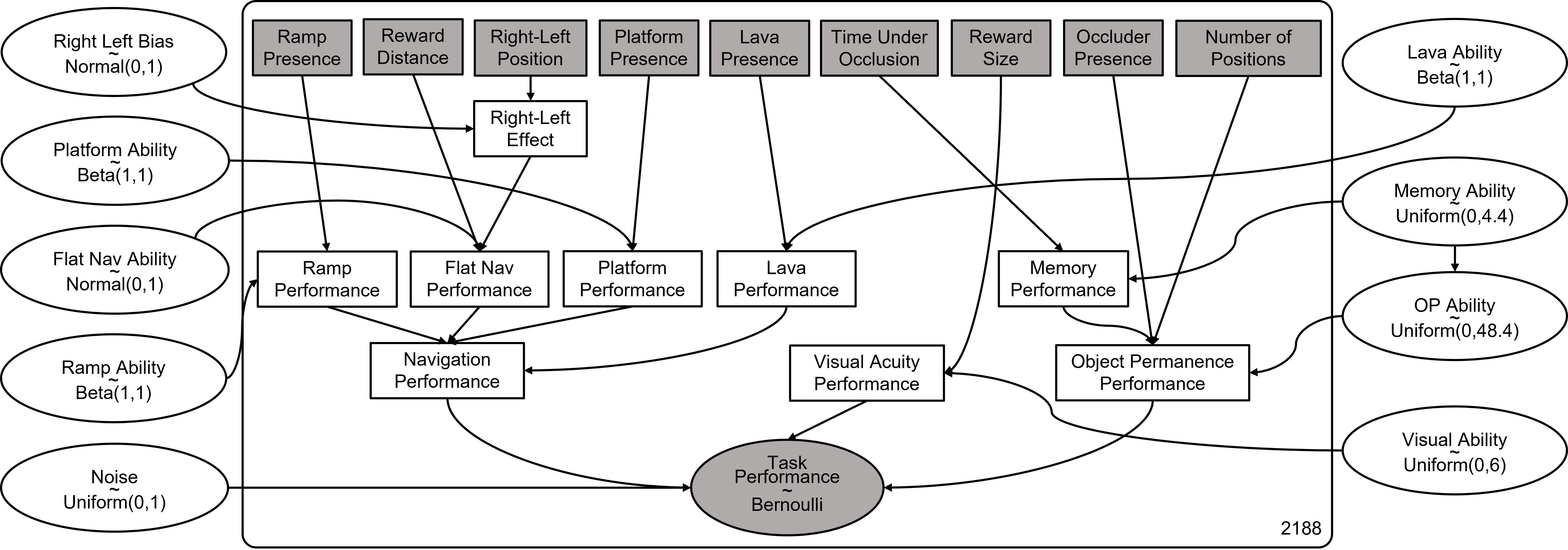
Figure 5: Visual representation of the measurement layout for the object permanence task.

Team A generated 30 synthetic agents of four different types to ensure a diversity of behaviour. Reference Agents act as reference points, e.g., a perfect agent, an agent with $x$% success, etc.

Achilles Heel Agents have low ability on some dimension, but otherwise perform well and can be said to have object permanence.

Context-Specific Agents have mixed OP performance, doing well in some specific tests/contexts but not others.

Fraudster Agents behave in a sophisticated manner that might look like object permanence, but actually is not (Uzgiris and Hunt 1975). Tables  6 and  7 in appendix D.4 show the specifics of each agent. This information was not disclosed to Team B.

5.2 Measurement Layout

Object permanence is a difficult capability to evaluate—combined with the need to visually identify goals, navigate to the goal, avoid hazards, and to remember the location of the object; there are many possible factors influencing overall performance that need to be disambiguated.

We present the measurement layout for the OP tasks in Fig. 5. The same broad structure as for the AAIO measurement layout is expanded upon. In the OP task-suite, there are additional challenges to navigation in the form of ramps, platforms, and lava. Subsequently, nodes for the agent’s capability (and instance-level performance) at handling each of these must be added to the layout. Meta-features for the presence of each of these challenges are needed. To represent object permanence specifically, we add extra meta-features: Occluder Presence, Time Under Occlusion, and Number of Positions (denoting the number of search-location choices available to the agent in forced choice instances). We further add capability nodes for Object Permanence and Memory Ability (each with an associated Performance node). Memory Performance, Occluder Presence and Number of Positions all feed into object permanence performance. The linking function for OP performance is the non-complementary product of Memory Performance and the logistic of the OP margin. The OP margin is the difference between Object Permanence and the product of Number of Positions and Time Under Occlusion. If no occluder was present the linking function for Object Permanence Performance returns $1$.

5.3 Inference and Analysis

Team B took the synthetic agent results and inferred the cognitive profiles using the PyMC implementation of the measurement layout. Overall, our model was successful at inferring system capabilities from patterns of performance. We evaluated the model in three ways. The first was a qualitative comparison of the cognitive profile descriptions generated by Team B with the criteria used to generate the agents. The model facilitated a correct description of the agent in around 75% of cases. For the “Achilles Heel” agents in particular, which had object permanence abilities but a specific weakness, the model was highly successful at identifying the cause of failure. It was, however unable to spot “fraudsters” making use of strategies (such as “go to the last seen location of the reward”) to mimic OP capability. Appendix D.4 contains a detailed breakdown of inferred parameters of the cognitive profiles of each agent, more information on the experimental set up, and the full qualitative analysis comparing inferred capabilities to the ground truth capabilities of the agents designed by Team A.

Capability	OP	FlatNav	Visual	Lava	Platform	Ramp	Memory
Overall RMSE	0.28	0.18	0.16	0.2	0.28	0.38	0.15
Included RMSE	0.13	0.11	0.24	0.17	0.134	0.27	0.16

Table 1: RMSE between the ground truth cognitive profile for Team A’s synthetic agents and the inferred values by Team B’s measurement layout. Overall: All 30 agents. Included: 13 agents generated using only the features included in the model.

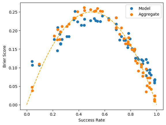
(a) AAIO Tasks

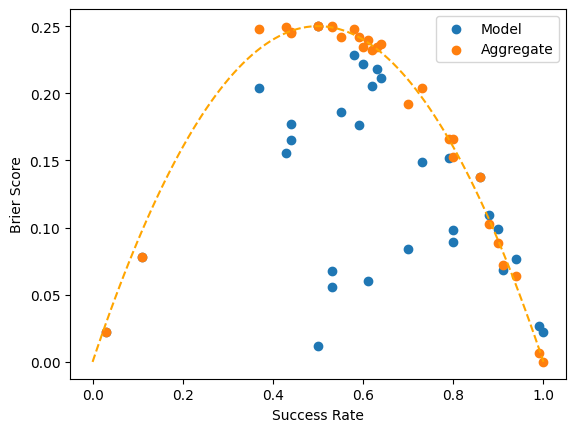
(b) O-PIAAGETS tasks.

Figure 6: Brier score of model predictions against agent success rates.

The second validation involved calculating the RMSE of the model for each ability (normalised to be in $[0,1]$), relative to the ground truth generated by Team A. Given in Table 1, model errors were modest across most abilities. Understandably, the model struggled most with agents that were created using features not captured by the model. For example, agent 23 was generated to have robust object permanence only in cup tasks (passing only 10% of other types). As our model did not include task type as a meta-feature, it erroneously took the non-cup task failures as evidence the agent lacks OP as well as struggling with platforms. However, given that the cup tasks are the only OP tasks without platforms, this is not an unreasonable assessment. By contrast, as the bottom row of the table shows, the model was accurate for agents generated using only features included in the model. This highlights the importance of having a measurement layout capturing the important meta-features that most affect performance, and also of designing test-batteries that allow confounding factors to be disentangled.

For our third validation, we show that our model can be used for accurate prediction of agent success on unseen task instances. Taking instance meta-features and applying forward inference with our model yields a probability of success. We compare this to the probability predicted by aggregate success using a Brier score. The full results are given in Appendix E, but a summary is given in Figure 6(b). The model is consistently a better predictor of success than relying on the aggregate measure. We see better prediction performance for agents with less certain success rates. These are the agents for which we are more interested in improving prediction as there is more capacity to reduce uncertainty.

6 Discussion

Increasingly more machine learning systems are (pre-)trained once and deployed for a range of tasks, Task-oriented evaluation based on aggregated performance cannot robustly evaluate these systems across the many situations in which they might be deployed, nor predict behaviour for new tasks and changing distributions. However, we can often identify abstract capabilities that are not directly measurable, such as ‘object permanence’ in agents or ‘handling negation’ in language models. In the behavioural sciences this is a common approach, but many techniques are populational. Triangulation for single individuals by contrasting against the task demands is common in animal cognition research, but it is unusual to see complex inferences from thousands of items, as is common in machine learning. In this paper we have integrated several elements to make this inferential exercise possible and shown it can identify the capabilities and biases of each model—its cognitive profile—independently.

This unleashes a new way of evaluating general-purpose systems, by identifying areas of weakness or reasons for task failure. This is especially useful for hierarchical capabilities with multiple levels of dependency. We can speed up the debugging process by isolating skill-gaps or biases responsible for failure, and improve confidence in predictions of performance on new tasks. Instead of hoping that the average performance will hold on new tasks, our approach enables the use of task demands and the inferred cognitive profile to determine whether system deployment is safe and worthwhile.

There are several limitations of this work. If many parameters must be inferred simultaneously then many evaluation instances are needed. We advocate incremental approaches, where each capability is inferred with subsets of tasks before moving to tasks with more complex dependencies. Nonetheless, we have shown that even a posteriori, as in the AAIO, inferences can be achieved simultaneously. Here we covered only the domain of agentic systems, but the same ideas can be extrapolated to language, vision and other domains. Ultimately, the biggest challenge for the construction of measurement layouts is the need for detailed domain knowledge and robust evaluation batteries. Both can be costly, but are urgently needed to improve AI evaluation. Currently, evaluation is focused on advancing SOTA performance on an increasingly small selection of benchmarks that often lack construct validity and are limited in scope (Koch et al. 2021; Raji et al. 2021).

Our approach also highlights the need for a clear distinction between training datasets, which can be massive, unannotated, and built in an adversarial way (Kiela et al. 2021) (Jia and Liang 2017; Zellers et al. 2019), and evaluation batteries, which should be devised carefully with systematic variation across the elements that might affect performance. Our vision is that, from well-constructed batteries such as O-PIAAGETS, building measurement layouts and triangulating with them should become routine.

Appendices

Here we include some supplementary material to the paper. First we include more details about PyMC, the Bayesian inference engine we are using and the decisions made for the estimation algorithm, and then we give more details and results for the two scenarios; first, the Animal AI Olympics and second, O-PIAAGETS.

Appendix A PyMC

PyMC (Salvatier, Wiecki, and Fonnesbeck 2016) is a probabilistic programming language for building Bayesian models and fitting them with Markov Chain Monte Carlo (MCMC) methods (Andrieu et al. 2003). Complex Bayesian models often require solving intractable integrals for inference such as the normalisation constant in Bayes’ theorem,

$$p(\theta|x)=\frac{p(\theta)p(x|\theta)}{\int p(\theta^{\prime})p(x|\theta^{\prime})d\theta^{\prime}}$$

among others. Monte Carlo (MC) Integration provides a method to approximate these intractable integrals using random sampling.

In order to evaluate

$$I=\int_{\Omega}f(x)dx$$

we can rewrite it as an expectation

$$I=\int_{\Omega}\frac{f(x)p(x)}{p(x)}dx\\ =\mathbb{E}\left[\frac{f(x)}{p(x)}\right]$$

for any density function $p$ such that $p(x)>0$.

MC Integration takes a random sample $X=\{x_{i}\}_{i=1}^{N}\in\Omega$ with distribution $p(x)$ and uses the Law of Large Numbers to approximate the integral as:

$$I\approx\frac{1}{N}\sum_{i=1}^{N}\frac{f(x_{i})}{p(x_{i})}$$

MC Integration is reliant on being able to sample efficiently from $\Omega$ according to $p(x)$. MCMC algorithms aim to do this, scaling to complex, hierarchical models by building a Markov Chain with equilibrium distributions approximating the desired probability density function $p$. Sampling from the Markov Chain can then be used as a stand-in for sampling $p(x)$. The prototypical example of an MCMC algorithm is the Metropolis Hastings algorithm (Hastings 1970). Hamiltonian Monte Carlo methods (Betancourt and Girolami 2013) improve on typical MCMC algorithms by replacing the random-walk element exploring the Markov Chain state-space with Hamiltonian Mechanics.

PyMC requires all expressions to be differentiable, which means that functions such as maximum and minimum are implemented as generalised means, and logical operators are implemented with products and sums.

A.1 Measurement Layouts in PyMC

In our work, we utilise the No U-Turn Sampler (Hoffman and Gelman 2014) built into PyMC, an extension to Hamiltonian MC methods which eliminates the need to set particular hyper-parameters.

With the NUTS sampler we use 2 sampling chains, tuned for $1000$ samples that are discarded in order to optimise the step-size within NUTS, and then draw $1000$ samples to estimate the posterior.

We define the model once for each scenario and then we estimate the parameters of the cognitive profile and some other INON elements for each system being evaluated independently.

As mentioned in the introduction, data and code will become available upon publication.

Appendix B Animal AI Environment and Competition

Animal-AI is an environment for training and testing AI systems. It is built in the Unity engine (Juliani et al. 2018). Animal-AI provides a first-person perspective in a 3D environment. The environment can contain a number of pre-specified objects, representing rewards, obstacles, tools, or dangers. Tasks can be defined using a domain-specific language to procedurally generate a large number of tasks instances. The agent’s interaction with the world is limited to moving around in the 3D space, though it can exploit physics interactions to exert more influence over the environment. Fig. 7 shows two screenshots from separate task instances.

In the Animal-AI Olympics (Crosby et al. 2020), an example arena containing the possible objects was provided to contestants. They were instructed that their agents would be evaluated on a variety of problems constructed from the objects in the example arena. The contestants then needed to build an agent—using any method of their choosing—that they believed would succeed at a wide variety of tasks. The tasks that ultimately made up the evaluation suite were based on adaptations of tasks from comparative and developmental literature. More information can be found at (http://animalai.org/AAI/).

For our work with the AAIO data-set we utilised a subset of tasks instances that were solvable with simple goal-directed behaviour. The specific task instances we utilised were:

[1-1-1, 1-1-2, 1-1-3, 1-2-1, 1-2-2, 1-2-3, 1-3-1, 1-3-2, 1-3-3, 1-4-1, 1-4-2, 1-4-3, 1-5-1, 1-5-2, 1-5-3, 1-6-1, 1-6-2, 1-6-3, 1-7-1, 1-7-2, 1-7-3, 1-8-1, 1-8-2, 1-8-3, 1-9-1, 1-9-2, 1-9-3, 1-10-1, 1-10-2, 1-10-3, 1-11-1, 1-11-2, 1-11-3, 1-12-1, 1-12-2, 1-12-3, 1-13-1, 1-13-2, 1-13-3, 1-14-1, 1-14-2, 1-14-3, 1-15-1, 1-15-2, 1-15-3, 1-16-1, 1-16-2, 1-16-3, 1-17-1, 1-17-2, 1-17-3, 7-1-1, 7-1-2, 7-1-3, 7-2-1, 7-2-2, 7-2-3, 7-3-1, 7-3-2, 7-3-3, 7-4-1, 7-4-2, 7-4-3, 7-5-1, 7-5-2, 7-5-3, 7-6-1, 7-6-2, 7-6-3]

The types of arenas that these instances correspond to can be found at (http://animalai.org/AAI/testbed).

Figure 7: Screenshots from two different instances in the Animal AI Olympics that we include in our analysis.

Appendix C AAIO Agent Results

This section gives more details for the first domain we examined in Section 4, the Animal-AI Olympics competition dataset. We also give more detail about the specifics of the measurement layouts.

C.1 Patterns of Performance

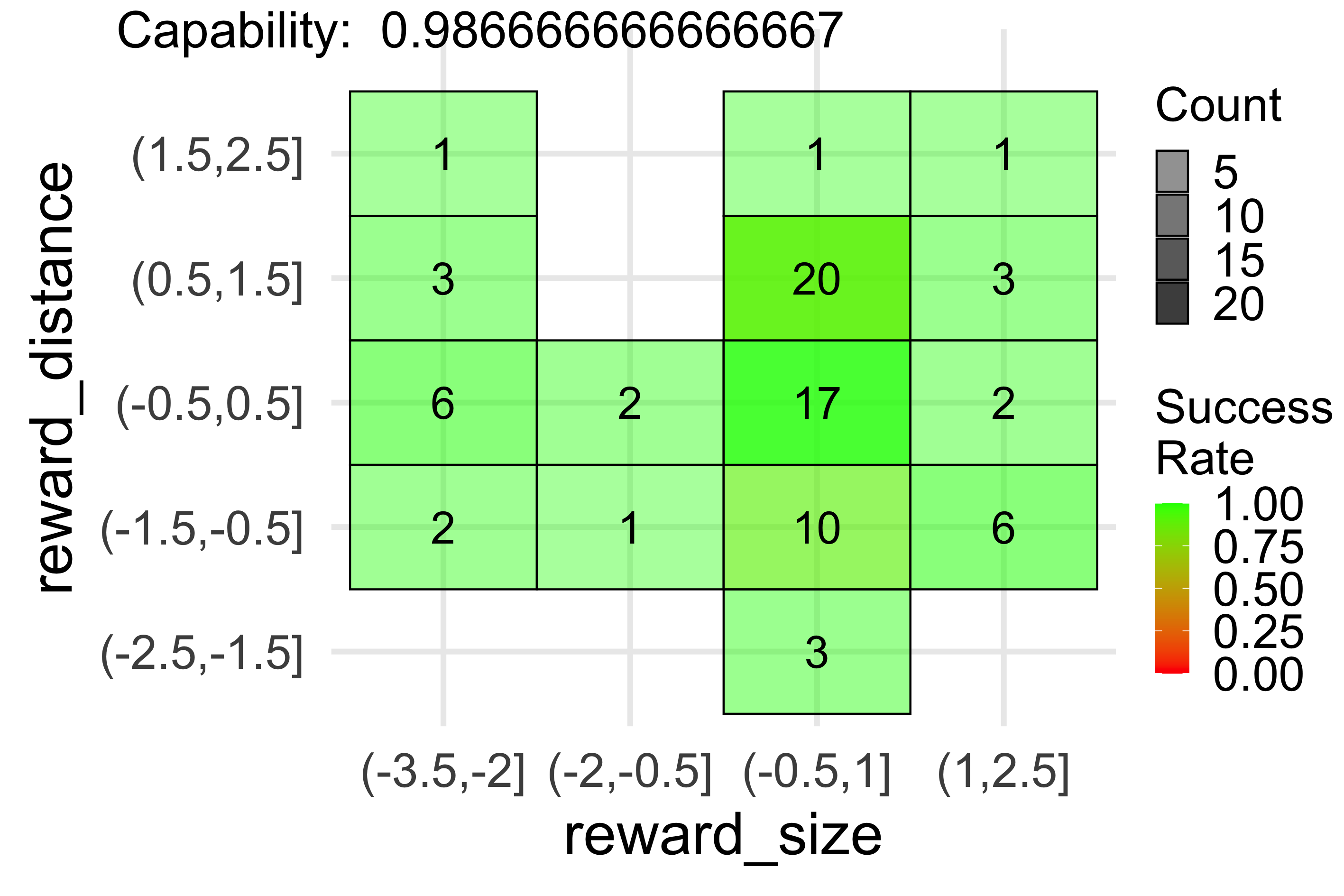
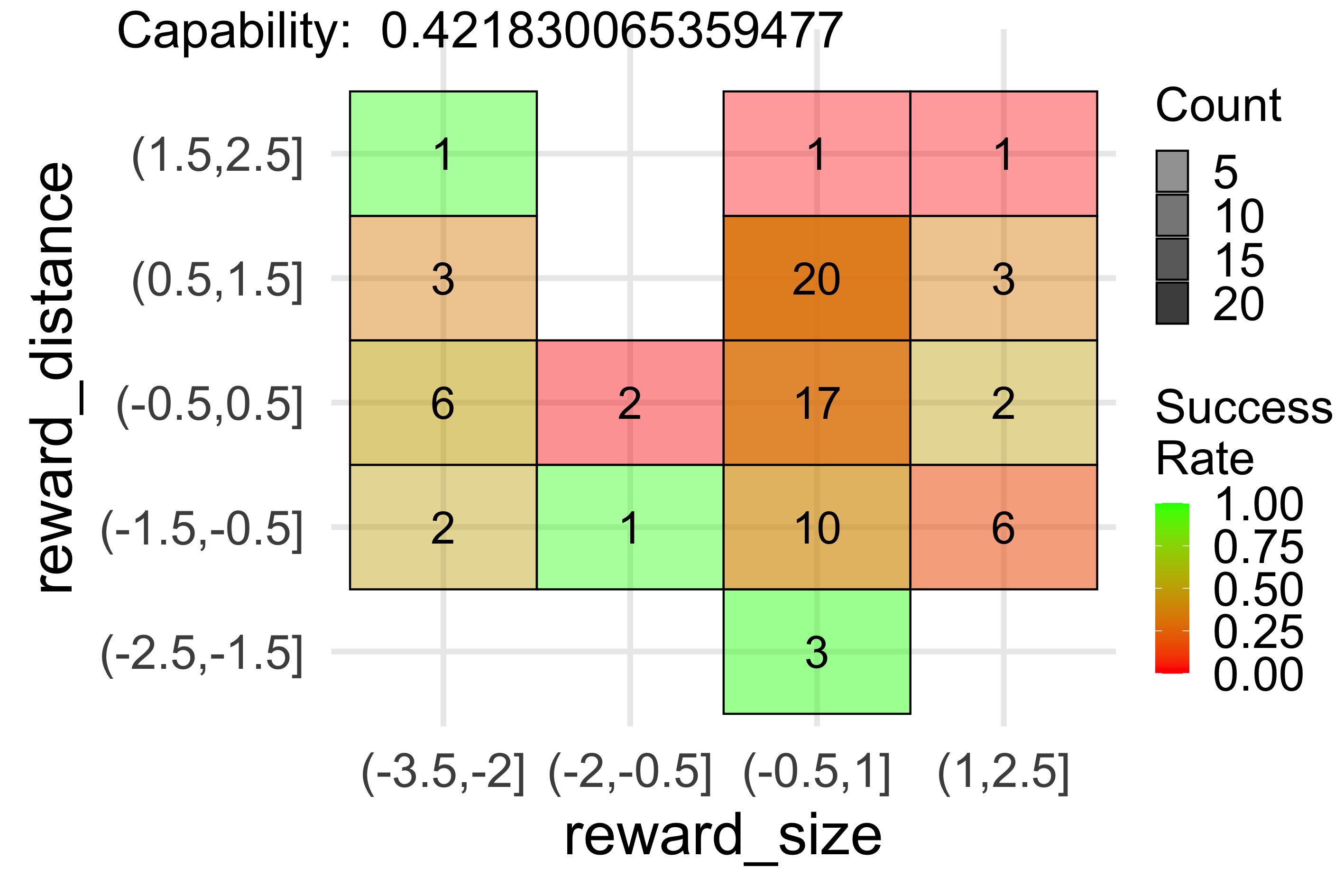
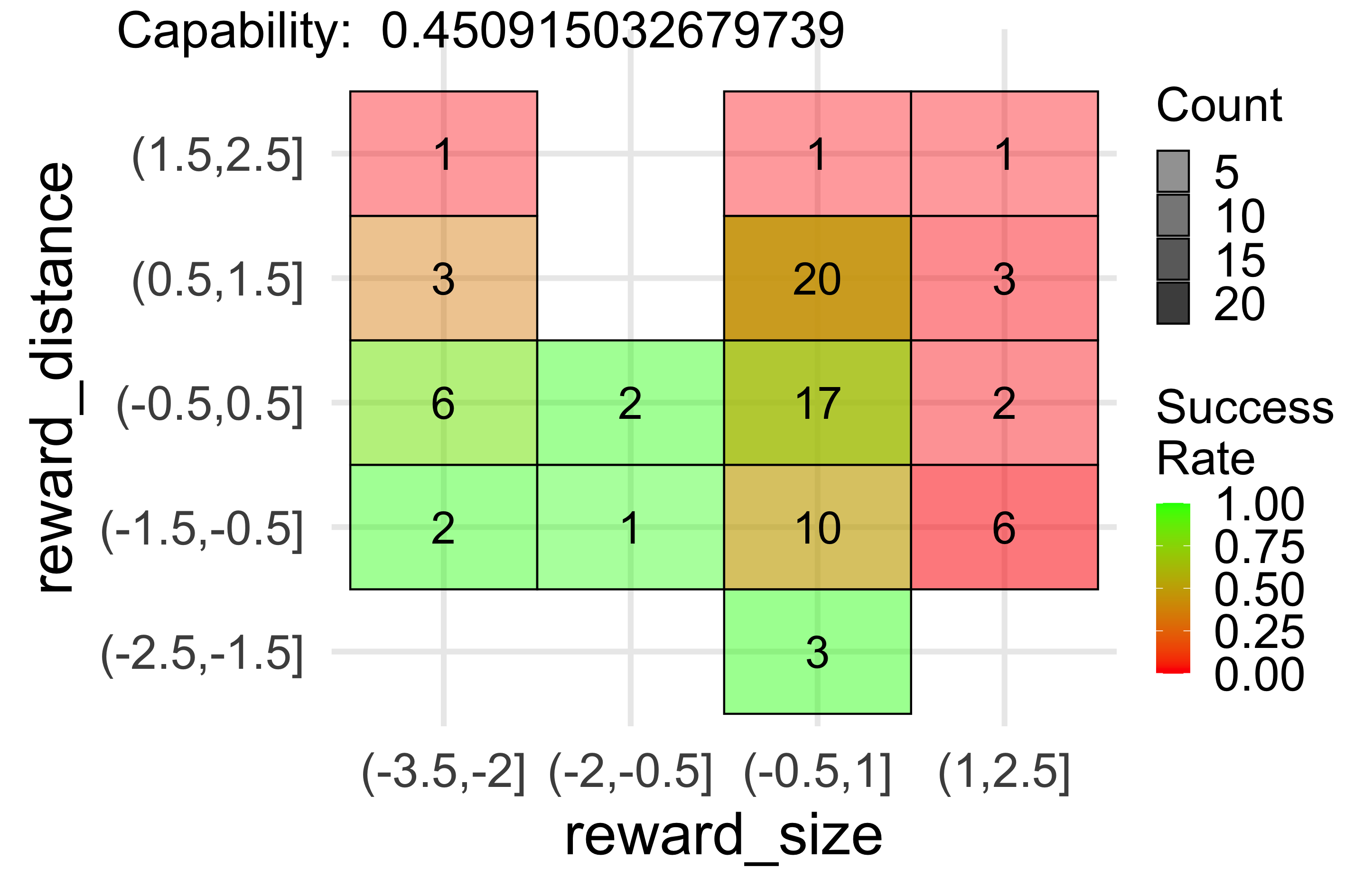
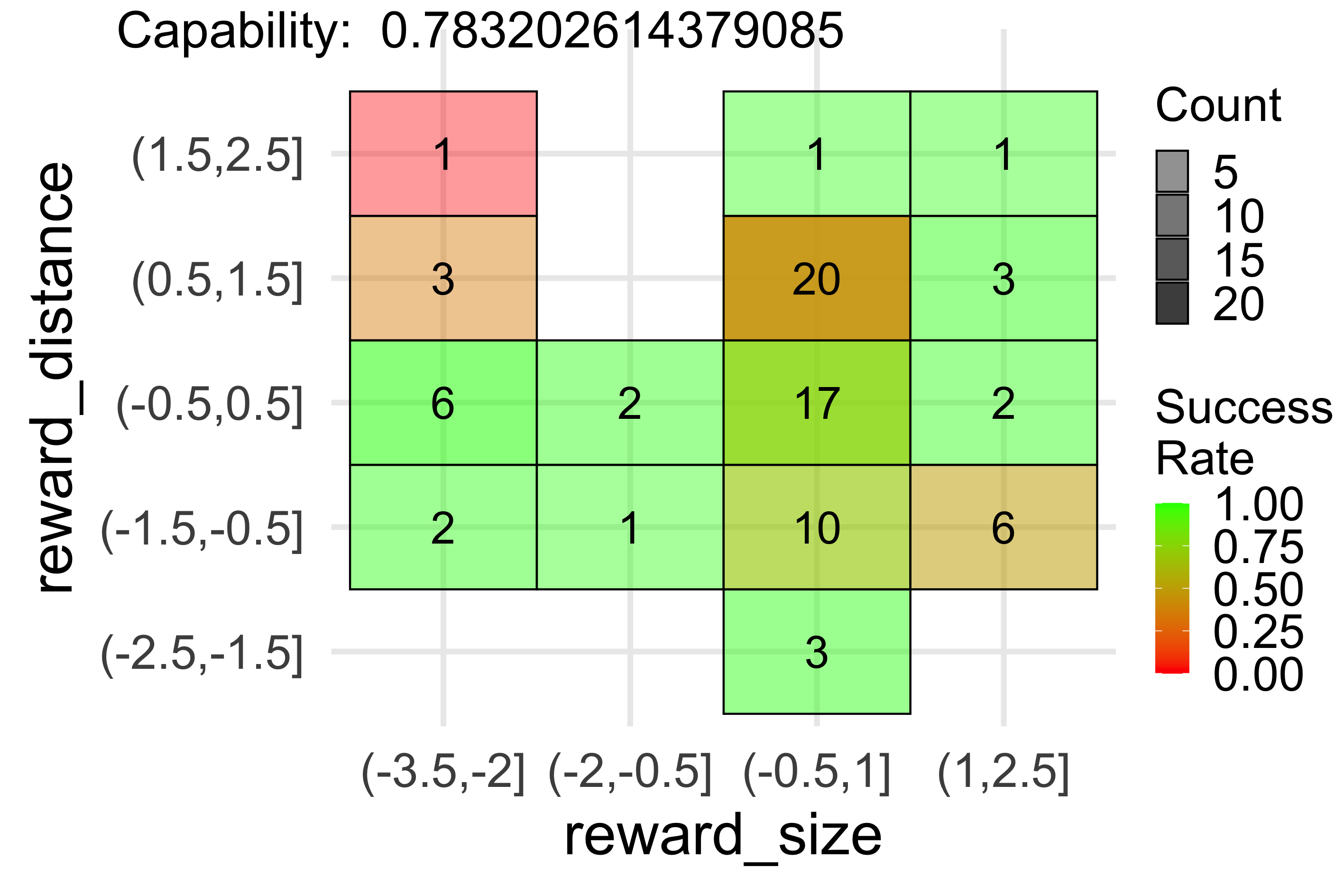
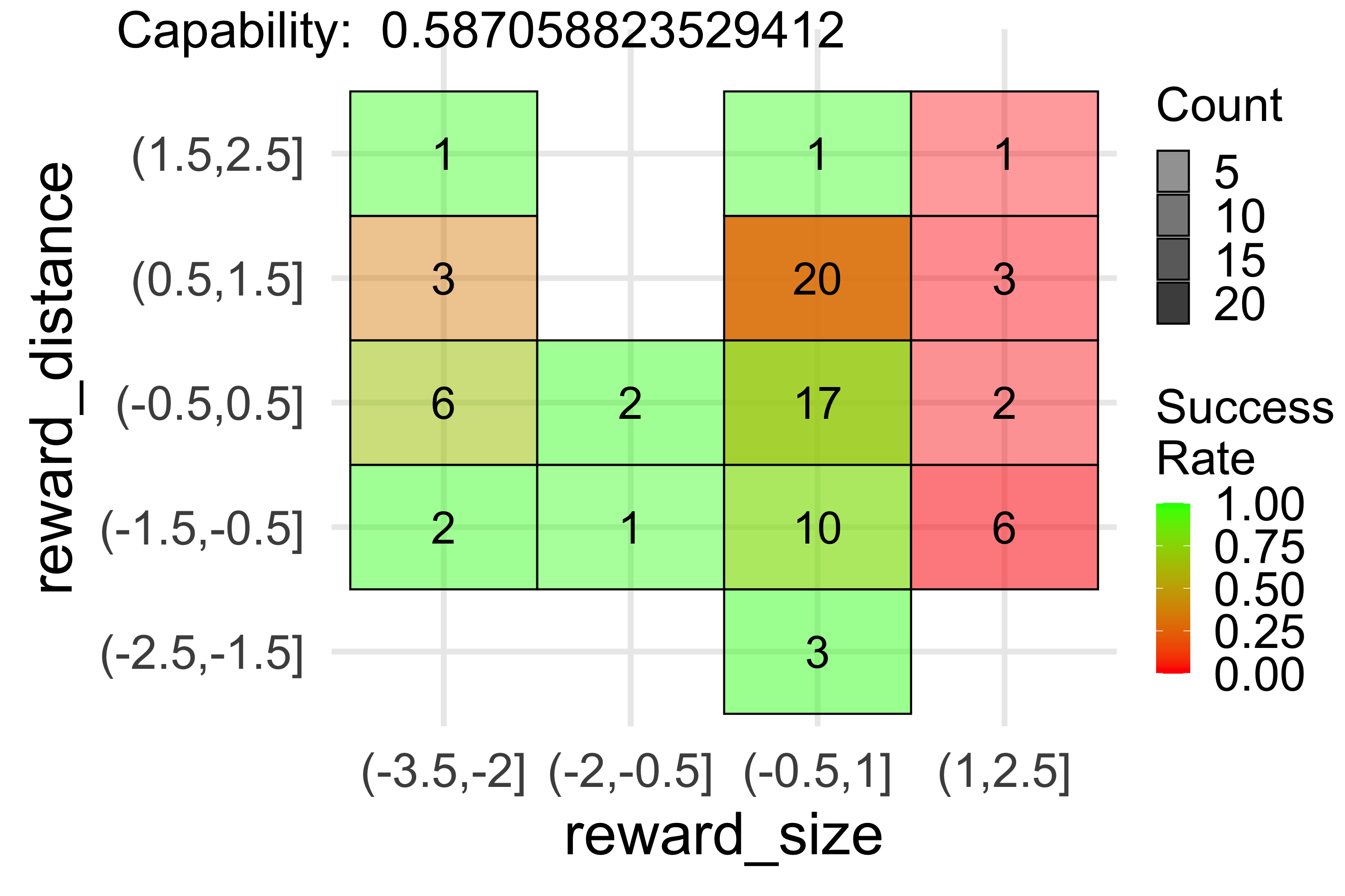
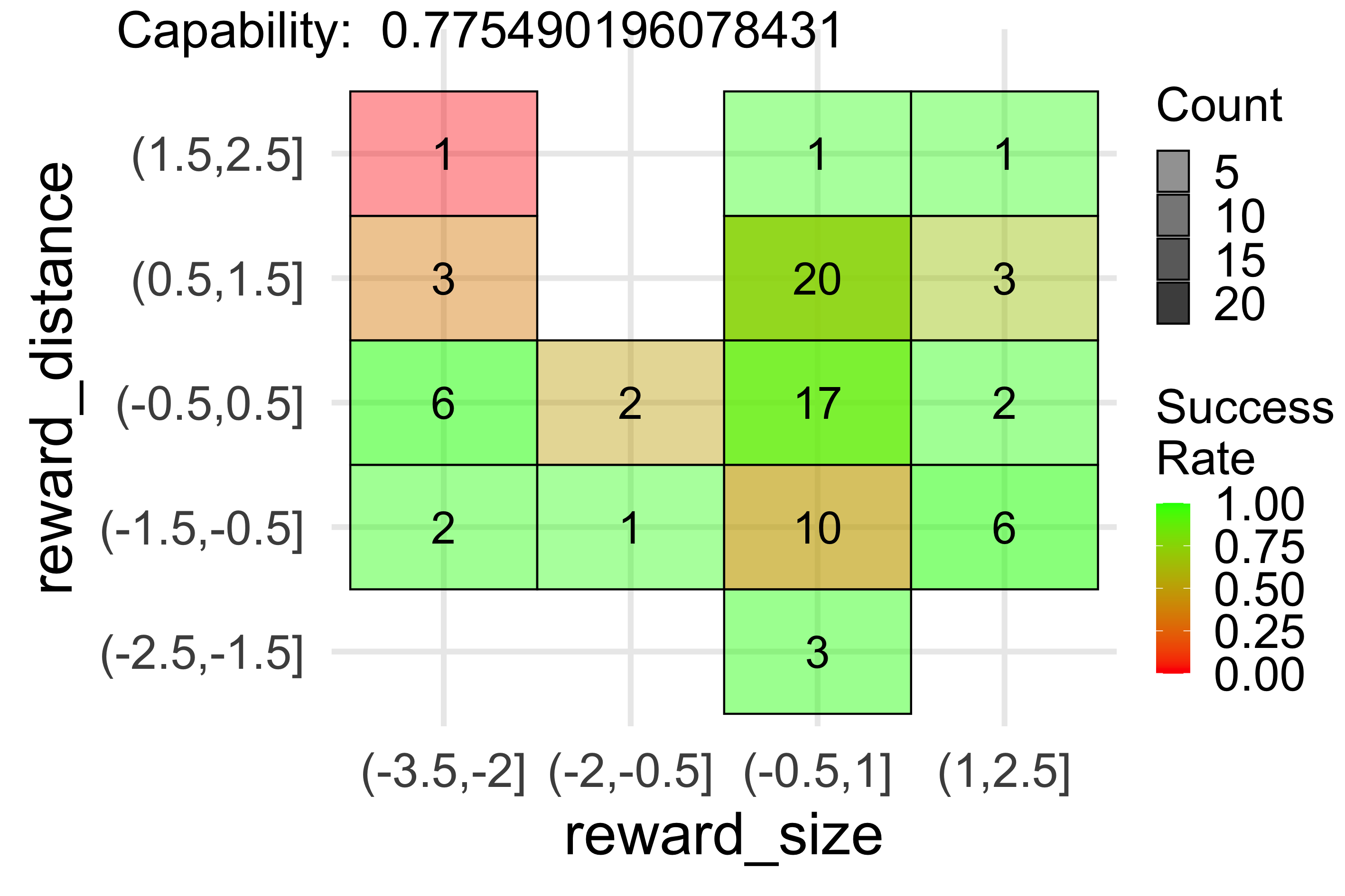
Figure 8: Agent characteristic grid displaying results for some selected agents. Top row, from left to right: ‘ironbar’, ‘sparklemotion’, ‘Juohmaru’. Bottom row, from left to right: ‘y.yang’, ‘daydayup’, ‘41Animals’. Note that the scales of the $x$-axis and $y$-axis are normalised and not the same as in the main body of text.

To show the patterns of performance of several agents, we use a simple visualisation known as agent characteristic grids, as described in (Burnell et al. 2022). The plots place each feature as a dimension and the success rate represented in colours from green (success) to red (failure). Values are grouped into bins of appropriate width in the desired dimensions for analysis. Each cell also shows the number of observed instances in that bin. Fig. 8 shows some of the agents discussed in the paper, as well as some other agents that will serve us to illustrate a few points.

For instance, ‘ironbar’ has 99% accuracy (the grid is mostly green everywhere) for this set of tasks (like ‘Trrrr’, the winner of the competition) and is identified as saturating both capabilities in Fig. 4. The next one, ‘sparklemotion’, with 36% accuracy, is very non-conformant, with navigationAbility $0.40\pm 0.38$ and visualAbility $0.59\pm 0.45$, and high noise $0.31\pm 0.13$. Proportionally, navigationAbility is worse as the grid looks even less conformant on the distance of the reward than the reward size. The rightmost on the top row is ‘Juohmaru’, with 54% accuracy, which is a very conformant agent, with red concentrating on the top and right of the grid (the objectively most difficult instances). Its navigation ability is $2.50\pm 1.08$ and visual ability is $0.92\pm 0.44$, and medium noise: $0.26\pm 0.17$.

We have specifically chosen some particular agents in the second row for which the extracted cognitive profile does not capture the whole performance patterns completely.

Leftmost on the second row, ‘y-yang’ has 70% accuracy and a very strange grid, with red cells in a diagonal, indicating a very non-conformant agent. This translates into navigationAbility $3.82\pm 0.45$ and visualAbility $1.68\pm 0.21$, but medium noise $0.22\pm 0.17$. This is so because overall the agent has high accuracy, so a bit of noise can explain the few anomalies on the top right of the grid.

In the middle of the second row is ‘daydayup’ with 52% accuracy. This agent shows a higher navigation ability than visual ability, as can be seen in the grid, where the size of the reward is the predictive feature and reward distance is less relevant. This translates into navigationAbility $3.48\pm 1.28$ (high than average but with uncertainty) and visualAbility $0.92\pm 0.44$ (low), with some a high level of random noise affecting performance $0.48\pm 0.20$.

Finally, ‘41Animals’ with 87% accuracy, shows relatively high values and low deviations for both navigationAbility $4.37\pm 0.59$ and visualAbility $1.81\pm 0.11$, with very little noise $0.05\pm 0.04$ despite having some non-conformant behaviour in the diagonal. In this case the left-right bias is higher ($0.45\pm 0.91$) and may account for this.

In general, for those agents where accuracy is too low or too high, the differences are more subtle. Of course, the interesting part of Fig. 9 is the agents in the middle. This suggests that estimating capabilities can benefit from a more focused analysis of instances around the demand thresholds. For ’Juohmaru’, this would amount to selecting instances by difficulty, instead of simply selecting all instances for analysis.

C.2 Animal AI Olympics Measurement Layout

Table 2 provides more information about the task meta-features that we utilised to construct the measurement layouts. Note that these ranges determine the ranges of the capabilities, so that we have units. For instance, if distance to the reward were measured in metres then the navigation capability would have metres as a unit. Let the navigation capability of an agent be, say, 20 metres. Since it is defined with a logistic function of distance, that means that the agent can achieve excellent performance when well below 20, performing at chance around the 20 metre mark, and failing every instance when the reward is well beyond 20 metres away.

Dimension	Description	Range/Values
Reward Size	The size of the reward (the sign is modified so lower is larger)	$[0,1.9]$
Reward Distance	Euclidean distance from the agent’s start position to the reward	$[0,5.3]$
Reward Behind	Whether the reward originates behind (1), left or right (0.5) or in front (0) of the agent	$\{0,0.5,1\}$
XPos	Whether the reward is to the left ($-1$), the right (1) or is centred (0) relative to the agent’s start position	$\{-1,0,1\}$

Table 2: AAIO Task Characterisation details. The dimensions on which instances vary in our measurement layouts.

Name	Type	Range/Values	Prior / Linking Function
rewardSize	Meta-Feature	$[0,1.9]$
rewardDistance	Meta-Feature	$[0,5.3]$
rewardBehind	Meta-Feature	$\{0,0.5,1\}$
XPos	Meta-Feature	$\{-1,0,1\}$
navigationAbility	Capability	$[0,5.3]$	$ScaledBeta(1,1,0,5.3)$
visualAbility	Capability	$[0,1.9]$	$ScaledBeta(1,1,0,1.9)$
rightleftBias	Bias	$[-\infty,\infty]$	$\mathcal{N}(0,1)$
noiseLevel	Robustness	$[0,1]$	$Uniform(0,1)$
rightleftEffect	INON	$[-1,1]$	${\sf rightleftBias}\times{\sf XPos}$
navigationPerformance	INON	$[0,1]$	$\sigma({\sf NavigationAbility}-{\sf rewardDistance}\times(\frac{1}{2}{\sf rewardBehind}+1)+{\sf rightleftEffect})$
visualPerformance	INON	$[0,1]$	$\sigma({\sf visualAbility}-{\sf rewardSize})$
taskPerformance	Observed	$[0,1]$	$p\sim Bernoulli(\omega[{\sf noiseLevel}]({\sf navigationPerformance}\times{\sf visualPerformance},\nu))$

Table 3: Nodes in the Animal AI Measurement Layout, including range/values, priors and linking function.

The measurement layout for this suite of tasks consists of two capability nodes (navigation and visual acuity), one bias node (whether the goal is initially on the left or the right of the agent), and one robustness node (stochastic noise on success/failure). Each of the capability and bias nodes has an associated instance-performance node, its intermediate non-observable node (INON). The noise is applied at the end.

In Table 3 we have complete details of all the nodes in the measurement layout. The function $\sigma$ represents the standard logistic function:

$$\sigma(x)=\frac{1}{1+e^{-x}}$$

while $\omega$ represents a weighting:

$$\omega[\alpha](b,c)=(1-\alpha)\cdot b+\alpha\cdot c$$

The value $\nu$ represents a noise prior that represents a constant model set to 1 $-$ average performance. Finally, $ScaledBeta$ represents a scaled beta distribution to an interval different from $[0,1]$. Note that a beta distribution has two parameters that need to be estimated.

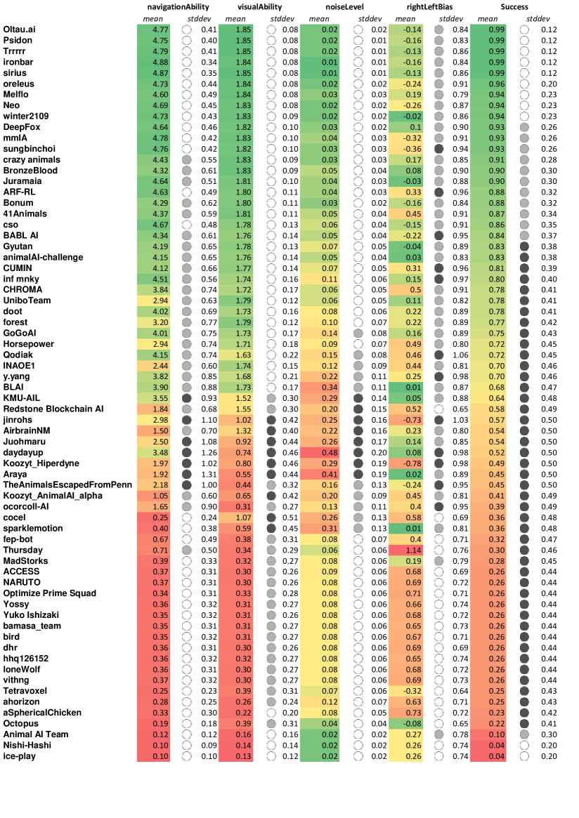
Figure 9: Inferred cognitive profile elements, along with the success rate, for the 68 agents in the AAIO. The gradient colour red-yellow-green denotes how high the means are (green is highest) while the gradient circles white-grey-black denote how high the standard deviations are (black is highest).

Finally, Fig. 9 shows the complete inference results for the 68 agents in the AAIO. The agents are ordered by the aggregate success rate at the collection of task instances. We see that, for the agents in the middle of the table in particular, our approach is able to decompose agent capabilities at this task into the constituent navigation and visual abilities. Bias has a more diverse behaviour throughout the table, with strong biases for extremely low scoring agents too, such as with agents ‘ahorizon’ and ‘Octopus’.

Equally, we can see that the detected bias can account for poor performance. Compare ‘Thursday’ and ‘MadStorks’ which share a similar overall success rate (0.30 vs. 0.28) despite the fact that ‘Thursday’ has much more navigation ability than ‘MadStorks’ and they have similar visual abilities. This is explained by ‘Thursday”s much larger bias towards moving to the right (0.73 vs 0.4) even if the reward is to the left.

Appendix D O-PIAAGETS Battery

Now we look at the object permanence test battery in more detail. We look at the overall design criteria for the test-bed, the types of tasks involved, and how the tasks are characterised. We also give full details for the measurement layout devised for this task and an extended view of the results inferred by our approach.

D.1 Design Criteria

Object Permanence (OP), and similar cognitive capabilities such as episodic memory and theory of mind, are difficult to robustly identify in AI systems because there are often several competing alternative explanations for why an agent is succeeding or failing at a particular task. We offer Bayesian triangulation as a solution to this problem.

Imagine a simple task where a reward is observed to roll leftwards behind an occluder, and go fully out of sight. An agent with OP ought to pass this task, since it: (a) wants to obtain the reward, (b) understands that the reward continues to exist despite not being able to see it, and (c) is able to infer the location of the occluded reward based on its previously observed trajectory. However, an agent with OP might fail this task, if for instance it is bad at navigating, and takes a very circuitous route to its goal and runs out of time before it can reach the reward. Conversely, an agent lacking OP might pass this task, simply because it has been rewarded previously for going forwards some number of steps and then turning left. This is the problem of the underdetermination of theory by behaviour (Stanford 2006), in which an observed behaviour can be explained in multiple ways. The use of well-informed measurement layouts based on internally valid test batteries allows us to more robustly eliminate incorrect alternative explanations and triangulate on the underlying causal explanations of AI system behaviour.

There are many competing desiderata to consider when designing a test-suite for the evaluation of OP in AI systems.

1. Cognitive capabilities such as OP can be difficult to place on an ordinal scale. This is because it is often not clear what affects behavioural performance in humans and other animals, and to what extent certain instance dimensions are relevant to good performance.

2. The relationships between cognitive capabilities can be complex and heterarchical, with single instances testing multiple cognitive capabilities with complex interactions. A carefully thought-out measurement layout is required, informed by cognitive science.

3. Instances may not be defined on all dimensions, introducing the possibility of missing data.

4. Instances are not necessarily evenly distributed across the levels of a dimension, leading to the potential for sampling biases.

These considerations were used as design criteria for the test-bed presented in the next subsection.

D.2 Object Permanence Tasks

The tasks that we use in our OP test-bed are based on a subset of the O-PIAAGETS object permanence test battery introduced in (Voudouris et al. 2022). The battery in its entirety is vast (including over 13,000 task instances requiring object permanence and over 250,000 basic task instances that don’t require OP, but help control for other potential explanations. Here, we adapt the following three separate task types from O-PIAAGETS.

Primate Cognition Test Battery Cup Tasks

Herrmann et al. developed the Primate Cognition Test Battery (PCTB) for testing aspects of physical and psychological common-sense in primates (Herrmann et al. 2007). One task in this battery was designed to assess OP. The participant is presented with three identical inverted cups, under which the experimenter hides a reward. Once the reward has been occluded, the participant is invited to lift a cup. If they fail to locate the reward, the trial ends. The reasoning here is that if the participant correctly locates the reward without any evidence of trial-and-error, there is evidence that they have OP, understanding that the reward continues to exist even when it is out of view.

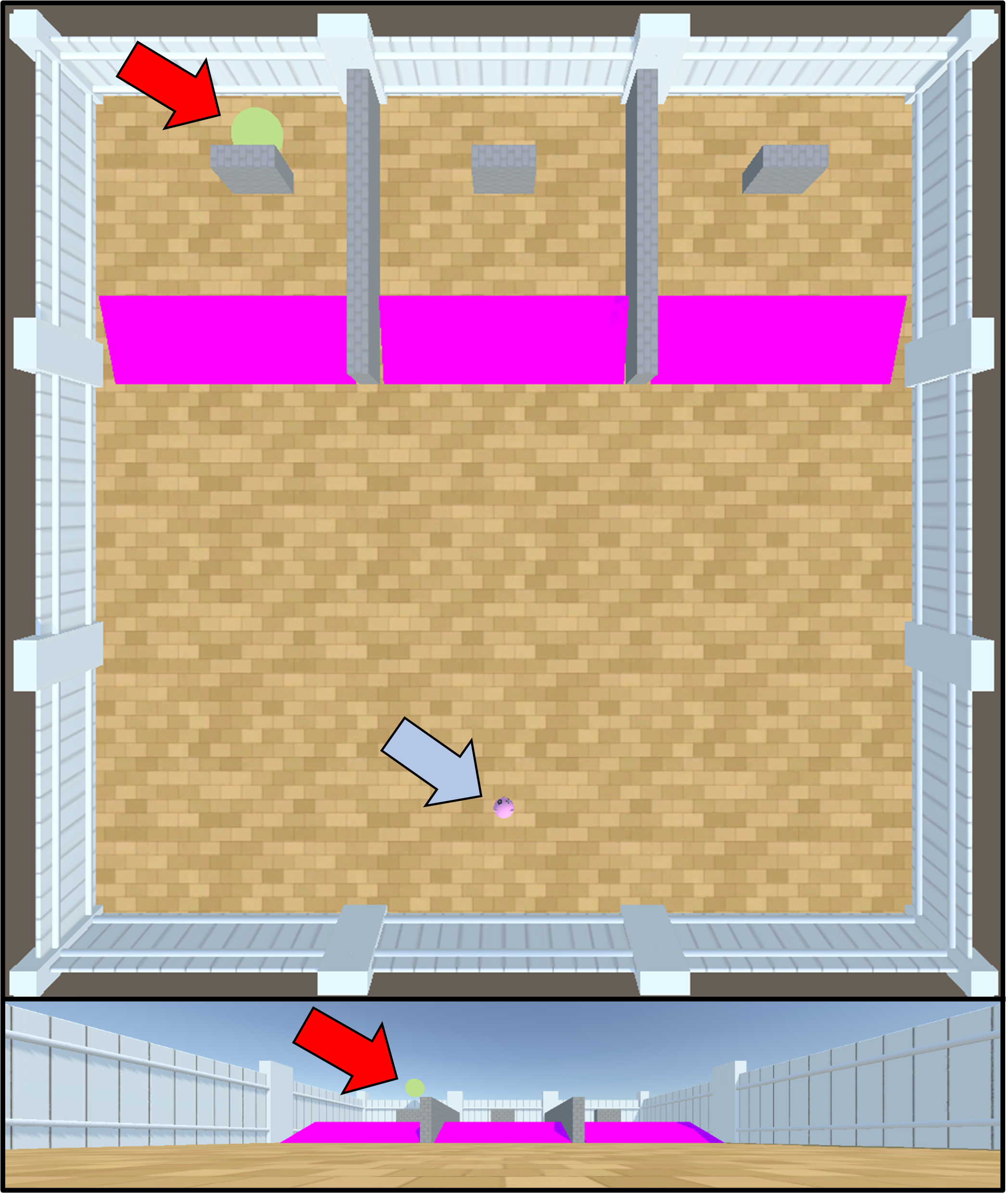
Figure 10: Primate Cognition Test Battery 3-Cup (’Cup’) Task. Top: Top-down view; bottom: Agent-view. Red arrow indicate reward location, grey arrows indicate agent location.

O-PIAAGETS has a battery of 598 instances based on this experimental set-up, including 359 that require object permanence to be solved and 239 that do not. In the OP tests, the agent observes a green reward drop from a height behind an occluder. They must traverse a ramp, sometimes avoiding lava, to obtain it. If they traverse the wrong ramp, they cannot return, and they will fail the instance, making this a forced choice test. See Fig. 10. In the instances that do not require OP, the reward is always visible, either through transparent objects or due to the lack of occluders. These instances serve as controls, so that we can evaluate whether poor performance on tasks requiring OP can be explained not by a lack of object permanence per se, but rather by poor performance traversing ramps, avoiding lava, or navigating towards rewards.

Primate Cognition Test Battery Grid Tasks

Extending the general structure for testing OP, Crosby et al. developed a task where rewards can be occluded in one of up to 12 different positions, through holes in the floor (Crosby et al. 2020). O-PIAAGETS contains 430 instances based on this design, with 4, 8, or 12 holes (see Fig. 11). 191 instances require OP to be solved, with the remaining 239 not requiring OP, where the holes are not deep enough to occlude the goal. These latter instances serve as controls.

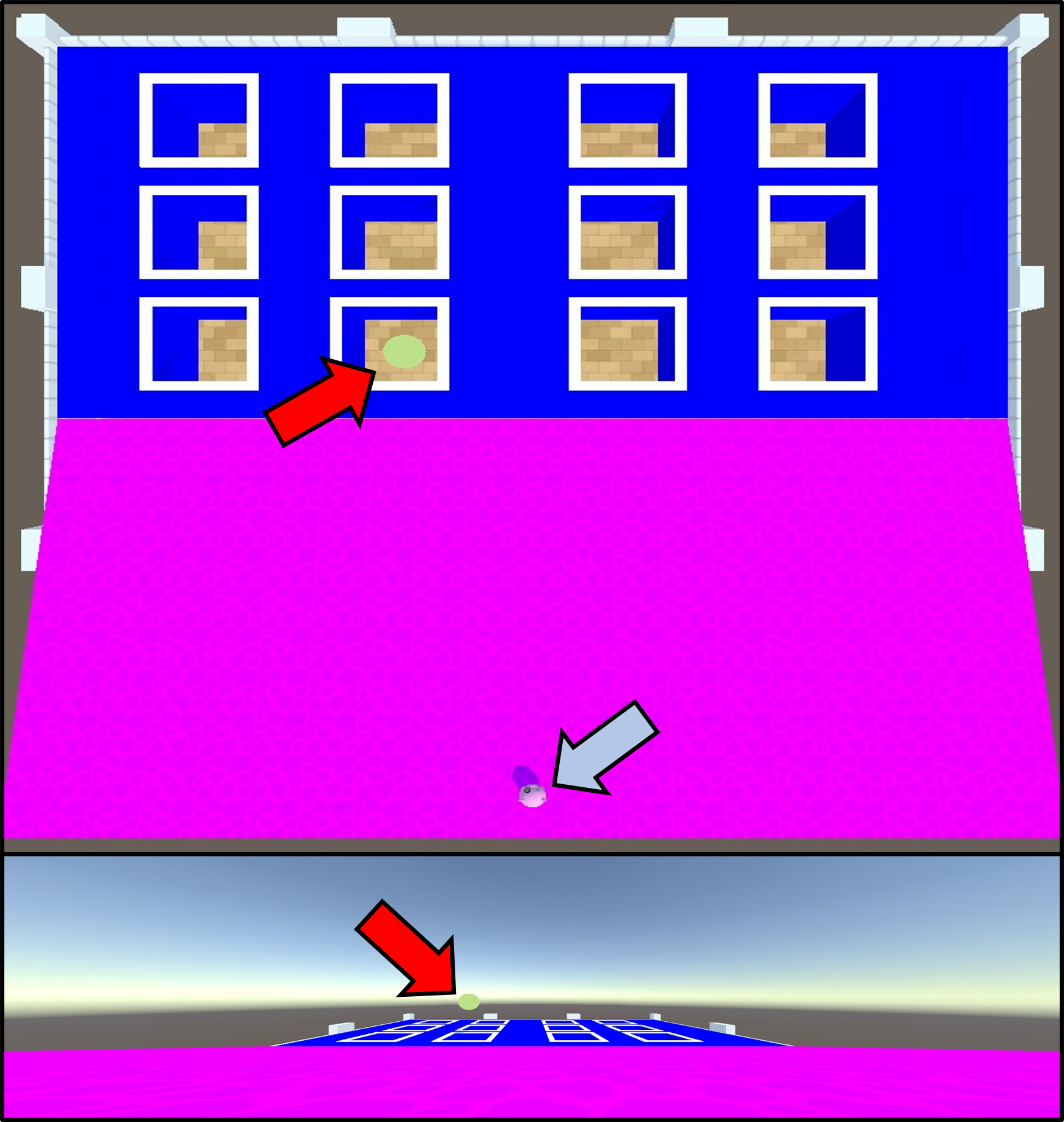
Figure 11: Primate Cognition Test Battery Grid (’Grid’) tasks. Top: Top-down view; bottom: Agent-view. Red arrow indicate reward location, grey arrows indicate agent location. Reproduced from Voudouris et al., 2022.

Chiandetti & Vallortigara Chick Tasks

Chiandetti and Vallortigara developed a series of tests for investigating physical common-sense in day-old chicks (Chiandetti and Vallortigara 2011), which Crosby et al. developed for use in the Animal-AI Environment (Crosby et al. 2020). In the example in Fig. 12, the agent observes a reward rolling away (panel A). Then the lights go out, blocking all visual input for several time steps (panel B). During this lights out period, the reward is deflected either left and rolls behind the occluder. When the lights turn on, the reward is fully occluded (panel C). If the agent understands that the reward continues to exist even when it is out of view, they ought to reason that it is behind the occluder on the left, as there is nowhere it could be hiding on the right.

Figure 12: Chiandetti and Vallortigara (’CV’) Task. Top: Reward Rolling away; middle: ”Lights out” period; bottom: Reward occluded. Reproduced from Voudouris et al., 2022

We used 36 instances from O-PIAAGETS that tested OP in this way, and included 1195 further tasks that did not require OP to be solved, to serve as controls.

Basic Tasks

All of these tasks require an agent to be able to navigate towards green goals, around obstacles, while traversing platforms and ramps, and avoiding lava. When testing for OP in biological agents such as primates or chicks, it is often safe to assume that they understand the value of rewards such as food or that they are able to navigate or search for rewarding objects. This is not a safe assumption when evaluating artificial agents, particularly those trained purely with techniques from machine learning. Therefore, the testbed must include instances that test for these basic skills. We included a further 521 instances testing basic abilities to navigate towards reward, avoid lava, and use ramps. These are extensions and variations of the tests used in section  4.

In total, we included 2188 unique instances from O-PIAAGETS, varying along the 12 dimensions outlined in Table  4. Note the asterisks in the table, denoting that a particular feature was not used in the measurement layouts used for evaluation in this paper. This occurred because Team B either didn’t realise the feature was present in the environment or because it was missed as a possible source of bias or capability. Nevertheless, this actually highlights a strength of our evaluation framework; imperfect measurement layouts can still be useful for both inferring agent capabilities and predicting future agent performance.

Dimension	Description	Range/Values
Reward Visibility*	Is the reward visible at the choice point?	${0,1}$
Time Under Occlusion	Time reward is occluded	$[0,4]$
Positions	Number of alternative reward places	$[1,11]$
Reward Distance	Manhattan distance to the goal	$[0,56]$
Right/left Position	Is reward left, right or straight from the agent?	$\{-1,0,1\}$
Reward Size	How large is the reward?	$[0.5,4]$
Occluder Presence	Are there any occluders hiding the rewards?	$\{0,1\}$
Lava Presence	Is there any lava in the arena?	${0,1}$
Platform Presence	Are there any platforms in the arena?	${0,1}$
Ramp Presence	Are there any ramps in the arena?	${0,1}$
Transparent Walls	Are there any transparent walls in the arena?	${0,1}$
Occluder Redness*	What is the R value of occluders in the arena?	$[0,255]$
Occluder Greenness*	What is the G value of occluders in the arena?	$[0,255]$
Occluder Blueness*	What is the B value of occluders in the arena?	$[0,255]$

Table 4: Object Permanence Task Characterisation details. The dimensions that instances vary on. The dimensions with an asterisk are not included in the measurement layout presented in this paper.

This test-bed satisfies our criteria for capturing and evaluating OP that we outlined above:

1. Object permanence is difficult to place on an ordinal scale. In cognitive science, it is usually discussed in terms of its presence or absence.

2. Object permanence relies on working memory capacity and spatial cognition, and successful performance on tests of OP often require good navigational skills. The dimensions defining each task vary on their relevance to OP and these precursor abilities (working memory, spatial cognition, navigational ability). There is therefore a complex interaction between latent capabilities and task dimensions.

3. Instances were not defined on all dimensions, introducing missingness. For example, in many instances, there were no occluders, so Occluder Colour is undefined.

4. Due to the structure of Animal-AI and O-PIAAGETS, some instance-types are represented more than others. For example, we have 36 Chiandetti & Vallortigara Chick Tasks testing OP, compared to 359 Primate Cognition Test Battery Cup Tasks, almost 10 times more.

D.3 Object Permanence Measurement Layout

This section extends the information about the measurement layout in section 5.2 and Fig. 5. The measurement layout for OP consists of seven capability nodes, one bias node, and one robustness node (stochastic noise on success/failure). As in the AAIO case, each of the capability and bias nodes has an associated instance-performance node, an intermediate non-observable node (INON). The noise is applied at the end to the final performance probability.

Name	Type	Range/Values	Prior/Linking Function
rampPresence	Meta-feature	$\{0,1\}$
lavaPresence	Meta-feature	$\{0,1\}$
platformPresence	Meta-feature	$\{0,1\}$
goalDistance	Meta-feature	$[0,56]$
goalSize	Meta-feature	$[0.4,5]$
rightleftPosition	Meta-feature	$\{-1,0,1\}$
occluderPresence	Meta-feature	$\{0,1\}$
timeUnderOcc	Meta-feature	$[0,4]$
mumberOfPositions	Meta-feature	$[1,11]$
OPAbility	Capability	$[0,48.4]$	$Uniform(0,48.4)$
memoryAbility	Capability	$[0,4.4]$	$Uniform(0,4.4)$
visualAbility	Capability	$[0,6]$	$Uniform(0,6)$
rampAbility	Capability	$[0,1]$	$Beta(1,1)$
lavaAbility	Capability	$[0,1]$	$Beta(1,1)$
platformAbility	Capability	$[0,1]$	$Beta(1,1)$
flatNavAbility	Capability	$[0,56]$	$\mathcal{N}(0,1)$
rightleftBias	Bias	$[-\infty,\infty]$	$\mathcal{N}(0,1)$
noiseLevel	Robustness	$[0,1]$	$Uniform(0,1)$
rampPerformance	INON	$[0,1]$	$\mu({\sf rampAbility},{\sf rampPresence})$
platformPerformance	INON	$[0,1]$	$\mu({\sf platformAbility},{\sf platformPresence})$
lavaPerformance	INON	$[0,1]$	$\mu({\sf lavaAbility},{\sf lavaPresence})$
flatnavPerformance	INON	$[0,1]$	$\sigma({\sf flatNavAbility}-{\sf goalDistance}+{\sf rightLeftEffect})$
navigationPerformance	INON	$[0,1]$	${\sf rampPerformance}\times{\sf platformPerformance}\times{\sf lavaPerformance}\times{\sf flatnavPerformance}$
memoryPerformance	INON	$[0,1]$	$\sigma({\sf memoryAbility}-{\sf timeUnderOcc})$
OPPerformance	INON	$[0,1]$	${\sf memoryPerformance}\times\sigma(48.4-((48.4-({\sf OPAbility}-{\sf 4}\times{\sf numPositions}))\times{\sf occluderPresence}))$
visualAcuityPerformance	INON	$[0,1]$	$\sigma({\sf visualAbility}-({\sf 5}-{\sf goalSize}))$
rightleftEffect	INON	$[-\infty,\infty]$	${\sf rightLeftBias}\times{\sf rightLeftPosition}$
taskPerformance	Observed	$[0,1]$	$p\sim Bernoulli(\omega[{\sf noiseLevel}]({\sf OPPerformance}\times{\sf navigationPerformance}\times{\sf visualAcuityPerformance},\nu))$

Table 5: Nodes in the Object Permanence Measurement Layout, including priors and linking function.

Table 5 gives the complete details, broken down by node type. As in the AAIO case, the function $\sigma$ is the standard logistic function while $\omega$ is a parameterised weighting function, where the value $\nu$ represents a noise prior that represents a constant model set to 1 $-$ average performance. The function $\mu$ is a margin, defined as

$$\mu(a,b)=1-((1-a)\cdot b)$$

where $a$ is an ability and $b$ a binary feature. This means that when the binary feature is 0 then the margin represents $p(success)=1$. If the binary feature = 1 then $p(success)=a$. The units of some of the abilities derive from the meta-features, like the memory ability, which is seconds, as it comes from the opposing metafeature timeUnderOcc. Similarly, visualAbility has the same units as goalSize, and flatNavAbility has the same units as goalDistance. OPAbility comes from a product between timeUnderOcc and numPositions so its unit is seconds times positions. Clearly, the most complicated linking function is the one for OPPerformance, which basically is opposed to (subtracted by) the maximum time under occlusion (4) times the number of positions. This is subtracted from the maximum OPAbility (48.4) and multiplied by the occluderPresence which is subtracted again from the maximum OPAbility (48.4). A logistic function is applied as usual but then this is multiplied by memoryPerformance, representing the dependency between object permanence and memory.

D.4 Synthetic Agents and Comparison

The synthetic agents Team A designed can be found in Table  6 and Table  7.

Name	Agent Class	Agent Description
Agent 1	Reference	Passes every instance.
Agent 2	Reference	Passes each instance with a probability of 0.5.
Agent 3	Reference	Passes each instance with a probability of 0.1.
Agent 4	Reference	Approximates a random walker. Passes a small proportion of instances. It is more likely to pass ’safe’ instances that don’t have lots of dangerous holes to fall down or lava to run into.
Agent 5	Reference	Passes each instance with a probability of 0.9. This is a more human-like failure rate than agent 1.
Agent 6	Achilles Heel	Has OP, passing an instance with a probability of 0.95 unless there is lava present, in which case it passes with a probability of 0.1.
Agent 7	Achilles Heel	Has OP, passing an instance with a probability of 0.95 unless there is lava or an occluder with a ‘redness‘ over 200 present, in which case it passes with a probability of 0.1.
Agent 8	Achilles Heel	Has OP, passing an instance with a probability of 0.95 unless there is an occluder with a ‘greenness‘ over 200 present, in which case it passes with a probability of 0.1.
Agent 9	Achilles Heel	Has OP, passing an instance with a probability of 0.95 unless there is a ramp present, in which case it passes with a probability of 0.1.
Agent 10	Achilles Heel	Has OP but lacks fine control of actions. If there is lava present, it only passes those instances with a probability of 0.5. It often falls into the wrong holes on its way to the further holes, so as distance to goal increases, the probability of passing Grid instances increases from 0.6 in increments of 0.1. This is only for the OP tasks. For the non-OP instances and the remaining instances, it solves an instance with a probability of 0.8.
Agent 11	Achilles Heel	Has OP but poor visual acuity. If goals are 0.5 or smaller, they only pass the instance with a probability of 0.1. For goals of size 1, the probability is 0.3, it is 0.5 for size 1.5, 0.7 for size 2, 0.8 for size 2.5, and 0.9 for a goal size 3 or larger.
Agent 12	Achilles Heel	Has OP but is biased to the right. Probability of passing a task is 0.95 when the goal is to the right, 0.3 when it is to the left, and 0.6 when it is centrally located.
Agent 13	Achilles Heel	Has OP but is biased to the left. Probability of passing a task is 0.95 when the goal is to the left, 0.3 when it is to the right, and 0.6 when it is centrally located.
Agent 14	Achilles Heel	Has OP, but is easily confused when there are several positions that are similar looking (either identical or mirror images of each other).
Agent 15	Fraudster	Does not have OP, but goes to where they last saw the reward. Deterministically passes all instances where this policy works (all tasks except some of CV Chick tasks), and fails the rest.
Agent 16	Fraudster	Does not have OP, but goes to where they last saw the reward. Passes all instances where this policy works with probability of 0.95 (all tasks except some of CV Chick tasks), and passes the rest with probability 0.25.

Table 6: The agents Team A designed and synthesised performances for.

Name	Agent Class	Agent Description
Agent 17	Achilles Heel	Has OP, but has low memory, so struggles when the goal is occluded for longer.
Agent 18	Achilles Heel	Has OP, but is easily confused when there are more positions that the goal could be occluded in. Passes instances with more than 10 other positions available with probability of 0.3. Between 5 and 10, probability of 0.6. Between 3 and 5, probability of 0.75. Less than 3, passes with probability of 0.95.
Agent 19	Context-Specific	Non-robust OP. It can solve the navigation tasks and all the CV tasks, but fails the other instances.
Agent 20	Context-Specific	Non-robust OP. It solves the navigation tasks and all the CV tasks with a probability of 0.75, fails the other paradigms with probability of 0.1.
Agent 21	Context-Specific	Non-robust OP. It can solve the navigation tasks and all the Grid tasks, but fails the other instances.
Agent 22	Context-Specific	Non-robust OP. It can solve the navigation tasks and all the Grid tasks with a probability of 0.75, fails the other paradigms with probability of 0.1.
Agent 23	Context-Specific	Non-robust OP. It can solve the navigation tasks and all the 3 cup tasks, but fails the other instances.
Agent 24	Context-Specific	Non-robust OP. It can solve the navigation tasks and all the 3 cup tasks with a probability of 0.75, fails the other paradigms with probability of 0.1.
Agent 25	Context-Specific	Non-robust OP. It can solve the navigation tasks and all the CV and grid tasks, but fails the other instances.
Agent 26	Cognitive Pathology	Non-robust OP. It can solve the navigation tasks and all the CV and grid tasks with a probability of 0.75, fails the other paradigms with probability of 0.1.
Agent 27	Cognitive Pathology	Non-robust OP. It can solve the navigation tasks and all the 3 Cup and grid tasks, but fails the other instances.
Agent 28	Cognitive Pathology	Non-robust OP. It can solve the navigation tasks and all the 3 cup and grid tasks with a probability of 0.75, fails the other paradigms with probability of 0.1.
Agent 29	Cognitive Pathology	Non-robust OP. It can solve the navigation tasks and all the CV and 3 cup tasks, but fails the other instances.
Agent 30	Cognitive Pathology	Non-robust OP. It can solve the navigation tasks and all the CV and 3 cup tasks with a probability of 0.75, fails the other paradigms with probability of 0.1.

Table 7: The agents Team A designed and synthesised performances for (continued).

Figs. 13 and 14 show the models inferred values for each element of the cognitive profile. Fig 13 gives the mean of the inferred distribution and Fig .14 the standard deviation. These values were used by Team B to infer the qualitative type of agent being evaluated. Multiple aspects of the values inferred by the model need to be considered to make a proper assessment of each agent—particularly since Team B did not know a priori the exact types of agents that would exist. For example, Agent 2 has relatively low scores for most abilities, a high standard deviation for most abilities, and a value of $0.5$ for the mean and s.d of overall success. This led Team B to believe that this agent was succeeding the tasks at random with 50% probability. Equally, when looking at Agents 13 and 14, the right-left bias was high (with low standard deviation) leading Team B to believe that these agents were massively favouring movement in particular directions.

In Fig. 15 we perform a qualitative comparison of the ground truth for the designed agents and the inferred profiles. The left side of the figure shows the ground truth characteristics of the agents generated by Team A. The right side of the figure shows Team B’s conclusions about the characteristics of the agents based on the outputs of the model. The colours denote how well Team B’s conclusions align with the ground truth, with green being more accurate and red being less accurate.

Using the measurement layout, Team B were able to recover all reference agents accurately. Team B were also able to recover the majority of the ‘Achilles Heel’ agents with high accuracy. Notable failures are the identification of a slight weakness with Lava for Agent 8 and a slight weakness with ramps for Agent 14. Agent 8 had a 90% probability of failing a task containing an occluder with a greenness value over 200, which has no bearing on the presence or absence of lava. It is possible that this small bias towards passing tasks without lava is a spurious result derived from the random values sampled to generate the performances. Agent 14 struggles with similar looking locations for reward locations, of which there are more for the grid tasks and the cup tasks, which both contain ramps by necessity, potentially explaining this ramp bias.

Team B were able to recover the cognitive profiles of Agents 17 and 18 to some degree. Team B inferred that Agent 17 struggled with memory, but because OP ability requires memory in the measurement layout, low memory ability was conflated with slightly lower OP. Agent 18 had worse performance when the reward could be hidden in more places. Similarly, the measurement layout stipulates that OP ability is required to track objects in multiple locations, so poorer performance on tasks with more hiding places was interpreted as a lower OP ability, a plausible inference.

Team B were able to partially recover the cognitive profiles of the context-specific agents. The relatively lower accuracy here was because task type was not included in the measurement layout. Therefore, many of the biases recovered by Team B reflect the particular construction of the paradigms used by Team A (see legend of Fig.  15).

Team B did not accurately recover the cognitive profiles of the ‘fraudster’ agents. Both Agents 15 and 16 follow the policy of going to where the goal was last seen. This results in generally good performance in all tasks except the Chiandetti & Vallortigara tasks, where this policy would result in falling into lava. Therefore, the performance distributions look similar to a high performing object permanence agent. To successfully discriminate these sophisticated agents, we would need to weight the importance of certain sub-groups of instances, such that, for example, Chiandetti & Vallortigara tasks are of most inferential importance in the case where there is good performance on the remaining paradigms. This requires targeted inference and diligent use and application of measurement layouts.

Overall, however, Team B was able to extract a lot of information about a the majority of the synthetic agents—despite an imperfectly designed measurement layout. Also noteworthy is that when the measurement provides correct inferences, they tend to be consistent across that particular agent. That is, if the measurement layout identifies a particular weakness in an agent, it won’t also pick a second, nonexistent weakness also.

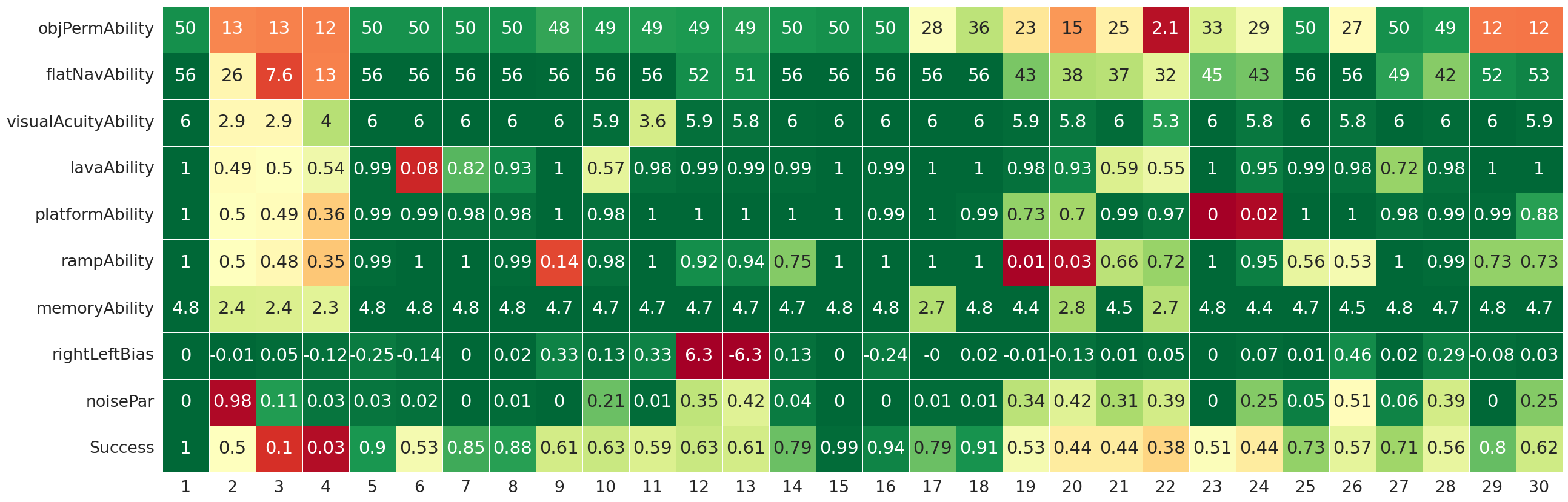
Figure 13: Mean inference results for the cognitive profile elements, along with the mean success rate, for the 30 synthetic agents in the OP task.

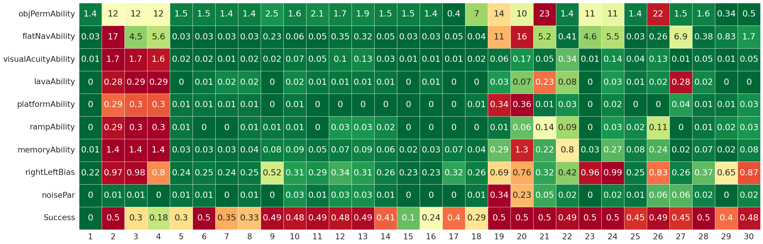
Figure 14: Standard Deviations of inferred cognitive profile elements, along with the standard deviation of the success rate, for the 30 synthetic agents in the OP task.

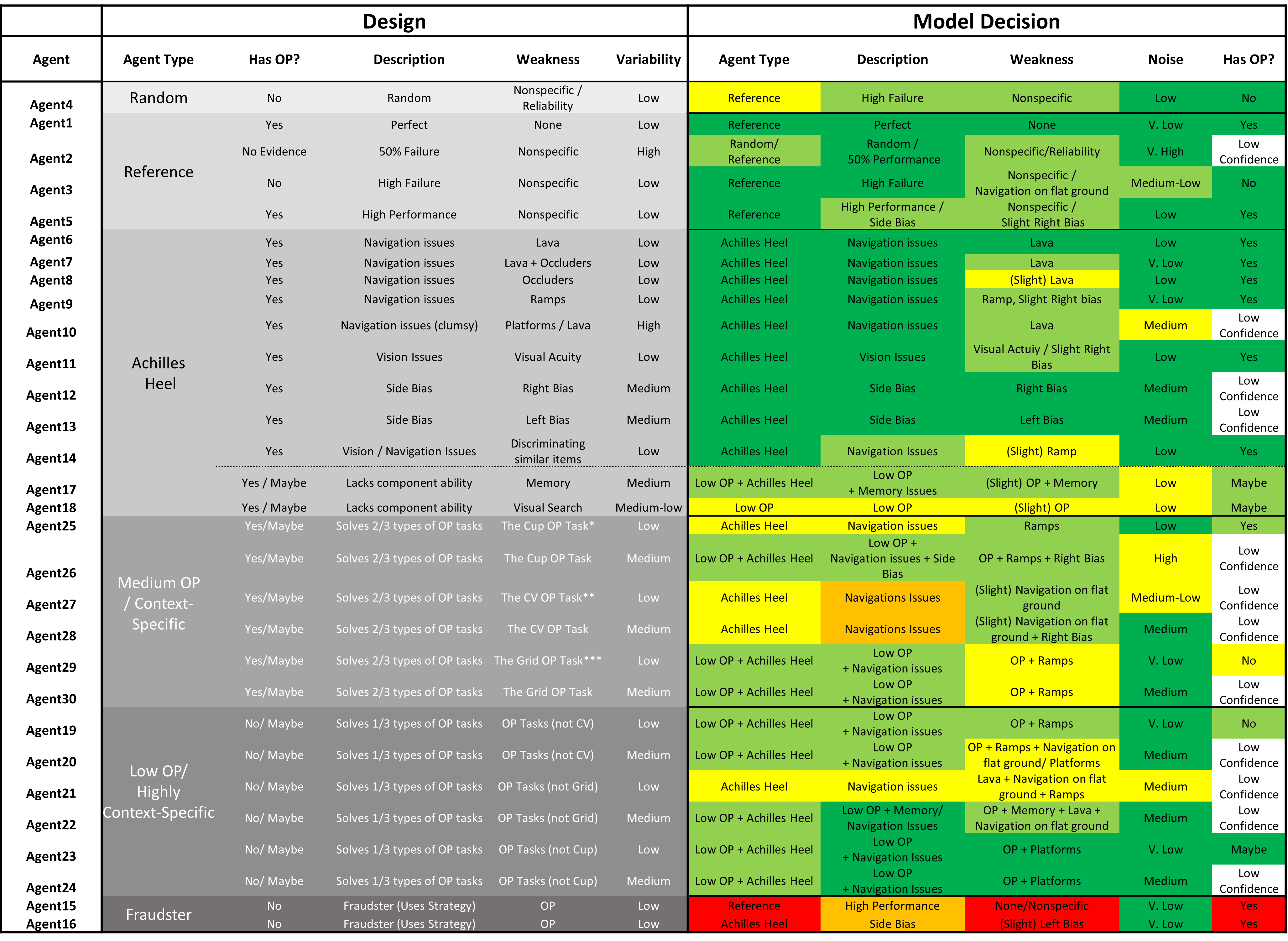
Figure 15: Qualitative analysis of the 30 synthetic agents, comparing the characteristics as they were designed with the cognitive profile that we have identified with our model decision for the measurement layout. In a gradient from green-yellow-red, with green representing a successful identification and red an unsuccessful one.

Appendix E Prediction Results

This section gives the full results for prediction on unseen instances. The synthetic data set was partitioned into an 80/20 train-test split. The measurement layout models (one for each agent) were trained on the same training partition. For each instance from the test-set we apply forward inference to yield a success probability.

We evaluate these probabilities using a Brier score (Brier 1950), also making use of the decomposition into Calibration and Refinement (Murphy 1973). These scores are given in Table 8, with the better performing approach for prediction in bold for each agent. As expected, the aggregate predictions have no refinement at all, and the values are close to 0.25 for balanced cases (the lower numbers only appear when the proportion of right/wrong performance is more imbalanced). The results from the measurement layout are much better here, as this method can give refined results per instance. When we look at calibration, however, we see aggregate predictions are almost perfect, since train and test come from the same distribution. But the calibration from the measurement layout is also quite good, and overall there are many more wins for the measurement layouts approach. Moreover, it is important to emphasise that unlike this table, train and test do not have to come from the same distribution. For instance, if we removed the easy instances for many of the tasks, we would get similar results for the measurement layout prediction approach (calibration and refinement should not change dramatically), but the results for the aggregate prediction approach would be much worse, since the calibration would be completely lost.

Looking at the particular agent properties that cause the measurement layouts to be more or less capable at prediction can provide some insight into the strengths and weaknesses of our approach. Agent 1 was designated as the perfect agent that will always pass every instance. It is no surprise then that predictions using the aggregate success rate were very successful, achieving the best possible Brier score. Our model’s predictions were still highly accurate (Brier score of 0.022), but the model lacked the extreme certainty of the aggregate measure—likely because using Bayes’ rule, beginning with an uninformed prior it’s impossible to update the posterior to exclude one of the outcomes.

Agent 5 is another case where the aggregate is better at prediction than our measurement layouts. Agent 5 passed all instances with probability 0.9. We believe our model struggled to perform as well as the aggregate here due to there not being sufficiently many instances to move the initial prior (uniform distribution) to the more extreme distribution predicting success at a rate of 0.9. Our model was able to cope with other fixed pass rates (such as with Agent 2, 3, and 4), so this may just be a matter of degree. It’s worth noting that for any fixed pass rate Agent, it’s actually impossible to predict more accurately than the aggregate in expectation. Hence For these types of agents the Aggregate Brier score is minimised, and for many fixed pass rate agents, our measurement layouts matched the aggregate’s Brier score.

Agents 7 and 8 were predicted equally or better by the Aggregate measure than our model. These agents passed all instances with probability 0.95, unless the object was occluded by an object with a lot of red or green present in its RGB colour value (red for 7, green for 8). Given that the measurement layout did not include colour values, it’s easy to see why they would struggle to predict this complex behaviour accurately. On the other hand, they did not do much worse than the aggregate prediction, with Brier scores of 0.138 vs 0.138 and 0.109 vs 0.103 respectively.

The only other agents that our measurement layouts were worse at predicting than the aggregate were agents 15 and 16. These two agents were designed as ‘Fraudster’ agents that mimic object permanence by going to the last position where they saw the reward. This is sufficient to solve many object permanence tasks except for some of the CV chick tasks. When this ‘Fraudster’ policy would be successful, these agents succeed with a probability of 0.95, if the policy would not be applicable, the agents succeeds with probability $0$ (for agent 15) or $0.25$ (for agent 16). We believe it is the high overall success rate that causes our model to be less predictive here, similar to Agent 5 (and to a lesser extent Agent 7 and 8), again because it takes more task instances to move an uninformative policy to extremes such as predicting success with a probability greater than $0.9$.

Agent	ML BS	Agg. BS	ML Cal.	Agg. Cal.	ML Ref.	Agg. Ref.
1	0.022	0.000	0.022	0.000	0.000	0.000
2	0.250	0.250	0.000	0.000	0.250	0.250
3	0.078	0.078	0.001	0.001	0.077	0.077
4	0.022	0.022	0.000	0.000	0.022	0.022
5	0.099	0.089	0.011	0.000	0.087	0.089
6	0.067	0.250	0.011	0.000	0.056	0.250
7	0.138	0.138	0.012	0.000	0.125	0.137
8	0.109	0.103	0.008	0.000	0.101	0.103
9	0.060	0.240	0.005	0.000	0.055	0.239
10	0.211	0.237	0.002	0.000	0.209	0.236
11	0.176	0.242	0.012	0.000	0.164	0.242
12	0.218	0.235	0.003	0.000	0.215	0.235
13	0.222	0.234	0.004	0.001	0.218	0.234
14	0.152	0.166	0.008	0.000	0.145	0.166
15	0.026	0.007	0.020	0.000	0.007	0.007
16	0.077	0.064	0.012	0.000	0.063	0.064
17	0.090	0.166	0.022	0.000	0.068	0.166
18	0.069	0.072	0.008	0.000	0.061	0.072
19	0.056	0.249	0.004	0.000	0.051	0.249
20	0.177	0.246	0.016	0.000	0.162	0.246
21	0.156	0.249	0.023	0.001	0.132	0.248
22	0.204	0.248	0.013	0.004	0.191	0.245
23	0.012	0.250	0.011	0.003	0.000	0.247
24	0.165	0.245	0.005	0.000	0.159	0.245
25	0.149	0.204	0.023	0.000	0.125	0.204
26	0.229	0.248	0.012	0.001	0.217	0.247
27	0.084	0.192	0.034	0.002	0.048	0.190
28	0.186	0.242	0.028	0.003	0.158	0.239
29	0.098	0.152	0.056	0.000	0.040	0.152
30	0.205	0.232	0.013	0.000	0.191	0.232

Table 8: Brier Scores (BS) and the breakdown into calibration (Cal.) and refinement (Ref.) for the Measurement Layouts (ML) and aggregate predictions (Agg.)

Appendix F Methodology for Designing Measurement Layouts

For complex, multifaceted tasks measurement layouts have the potential to grow and become large and complex themselves. It’s therefore important that to apply them to other domains (and reap the benefits of the additional evaluation information they provide) to have a general methodology for constructing the appropriate measurement layout structure. To this end, we developed a methodology for constructing measurement layouts that we wish to explicate here more clearly.

As stated in the main paper, the core of our approach is to identify the demands of a task, and to compare these against the capabilities of the system being evaluated. Tasks are composed of multiple instances that vary in the degree of demands. In our methodology we tie demands with meta-features in order to give the demands values that are tied to objective properties of the task. For each demand in a task, a system will have varying levels of performance at dealing with the demand based on its capability. we model this as a probability of the system successfully handling the aspect of the task with its meta-feature value. This is where the linking function comes into play. We often leveraged the sigmoid function $\sigma(capabiltiy-demand)$. This approach is beneficial because it ties capabilities to probabilistic performance based on the demand. This also causes the capabilities to have the same unit as the demand, and allows us to interpret a capability with value $x$ as consistently succeeding on the demand with meta-feature $x$ in $50\%$ of instances.

Certain demands also require that other demands have been met. This requires a dependency understanding of the demands of the task. Performances for dependent task demands can be incorporated into the sigmoid margin calculation or can have an effect on the resulting performance value. The exact approach for combining demand performances will depend on the task itself, and whether the demands are compensatory—whether performance can be achieved with one capability compensating for lacking another. Our environments were non-compensatory, so we often opted for taking the product of probabilities. However, more complex relations such as taking the minimum or maximum of a set of probabilities is available by utilising a generalised mean. The other major aspect that we need to identify to construct the measurement layout is the sources of possible bias. In principle, this is similar to creating the structure for capabilities: We still identify meta-features that may affect performance, however, now we are looking for those that are not necessary for the task. We still include a bias ”performance” for each instance (how present was the bias in this instance, and in which direction was it directed?) , but this is now included in the sigmoid function for the relevant capability it may affect: $\sigma(capability-demand+bias)$. Once all of the demands and biases are accounted for, a final combination can give an output for overall task performance.

Breaking a complex task down into demands and possible biases is not always straightforward. Care, and domain knowledge of what constitutes success in the task, needs to be utilised to identify the core broad capabilities required, and how these break down to identifiable meta-features. We recommend an iterative approach: If a particular measurement layout cannot explain system behaviour reliably (with a low standard deviation on the resulting posterior distributions), then there is either too few evaluation instances, or the measurement layout is missing an important capability or bias.

When evaluating Artificial Intelligence systems, and for that matter non-human Biological Intelligences, we need to be careful to avoid anthropomorphising the system. We do not want to mistakenly ascribe capabilities or explain behaviours based on a crude facsimile of human behaviour. AI systems, in particular, have the potential to solve tasks using incredibly different internal methods and skills. We have been careful to avoid this mistake in our work by focusing on the required demands for a task rather than any model for how the system internally processes meta-features.

Appendix G Computation Code, and Datasets

Our experiments did not require a large amount of compute, We ran all of our experiments on Google Colaboratory (Google 2017) using the free tier of service without utilising the GPU. All corresponding code, datasets and raw results will be released on publication to ensure ease of replication.

References

- Andrieu et al. (2003) Andrieu, C.; de Freitas, N.; Doucet, A.; and Jordan, M. I. 2003. An Introduction to MCMC for Machine Learning. Machine Learning, 50(1-2): 5–43.
- Baillargeon et al. (2011) Baillargeon, R.; Li, J.; Gertner, Y.; and Wu, D. 2011. How do infants reason about physical events?
- Ben-Gal (2008) Ben-Gal, I. 2008. Bayesian Networks. John Wiley & Sons, Ltd. ISBN 9780470061572.
- Bergman and Andersson (2015) Bergman, L. R.; and Andersson, H. 2015. The person and the variable in developmental psychology. Zeitschrift für Psychologie/Journal of Psychology.
- Betancourt and Girolami (2013) Betancourt, M.; and Girolami, M. 2013. Hamiltonian Monte Carlo for Hierarchical Models. arXiv 1312.0906.
- Brier (1950) Brier, G. W. 1950. Verification of Forecasts Expressed in Terms of Probability. Monthly Weather Review, 78(1): 1.
- Burnell et al. (2022) Burnell, R.; Burden, J.; Rutar, D.; Voudouris, K.; Cheke, L.; and Hernández-Orallo, J. 2022. Not a Number: Identifying Instance Features for Capability-Oriented Evaluation. IJCAI.
- Burnell et al. (2023) Burnell, R.; Schellaert, W.; Burden, J.; Ullman, T. D.; Martinez-Plumed, F.; Tenenbaum, J. B.; Rutar, D.; Cheke, L. G.; Sohl-Dickstein, J.; Mitchell, M.; Kiela, D.; Shanahan, M.; Voorhees, E. M.; Cohn, A. G.; Leibo, J. Z.; and Hernandez-Orallo, J. 2023. Rethink reporting of evaluation results in AI. Science, 380(6641): 136–138.