A structure-preserving finite element method for the multi-phase Mullins-Sekerka problem with triple junctions

Abstract

We consider a sharp interface formulation for the multi-phase Mullins-Sekerka flow. The flow is characterized by a network of curves evolving such that the total surface energy of the curves is reduced, while the areas of the enclosed phases are conserved. Making use of a variational formulation, we introduce a fully discrete finite element method. Our discretization features a parametric approximation of the moving interfaces that is independent of the discretization used for the equations in the bulk. The scheme can be shown to be unconditionally stable and to satisfy an exact volume conservation property. Moreover, an inherent tangential velocity for the vertices on the discrete curves leads to asymptotically equidistributed vertices, meaning no remeshing is necessary in practice. Several numerical examples, including a convergence experiment for the three-phase Mullins-Sekerka flow, demonstrate the capabilities of the introduced method.

Keywords - Mullins-Sekerka, multi-phase, parametric finite element method, unconditional stability, area preservation

1 Introduction

In this paper, we consider the problem of networks of curves moving under the multi-phase Mullins-Sekerka flow, see e.g. [13]. These networks feature triple junctions, at which certain balance laws need to hold. The network depicted in Figure 1 consists of three time dependent curves $\Gamma_{i}(t)$, $i=1,2,3$, that meet at two triple junction points $\mathcal{T}_{1}(t)$ and $\mathcal{T}_{2}(t)$. We assume that the curve network $\Gamma(t):=\cup_{i=1}^{3}\Gamma_{i}(t)$ lies in a domain $\Omega\subset\mathbb{R}^{2}$, and it partitions $\Omega$ into the three subdomains $\Omega_{j}(t)$, $j=1,2,3$. The three domains correspond to different phases in the multi-component system. The evolution of the interfaces $\Gamma_{1}(t),\Gamma_{2}(t),$ and $\Gamma_{3}(t)$ is driven by diffusion. As in [13], given a time $T>0$ and the hyperplane $T\Sigma:=\{\mbox{\boldmath{$u$}}\in\mathbb{R}^{3}\mid\sum_{j=1}^{3}u_{j}=0\}$, we introduce a vector of chemical potentials $\mbox{\boldmath{$w$}}:(0,T)\times\Omega\to T\Sigma$ which fulfills the quasi-static diffusion equation for $j=1,2,3$ and $t\in(0,T)$,

$$\Delta\mbox{\boldmath{$w$}}={\bf 0}\ \ \mbox{in}\ \ \Omega_{j}(t)$$ (1.1a)

together with

$$\partial_{\vec{\nu}_{\Omega}}\mbox{\boldmath{$w$}}={\bf 0}\ \ \mbox{on}\ \ \partial\Omega,$$ (1.1b)

where $$\vec{\nu}_{\Omega} \partial\Omega$$ denotes the outer unit normal vector to .

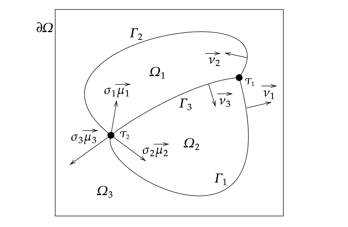
Figure 1: Three open curves with two triple junctions.

To close the system, we need boundary conditions on $\Gamma(t)$ and on $\mathcal{T}_{1}(t)$ and $\mathcal{T}_{2}(t)$. These boundary conditions are given by a Stefan-type kinetic condition and the Gibbs-Thomson law on the moving interfaces, and Young’s law at the triple junctions, see [13]. The kinetic condition reads

$$[\nabla\mbox{\boldmath{$w$}}]\vec{\nu}=-V[\mbox{\boldmath{$\chi$}}]\ \ \mbox{on}\ \ \Gamma(t),$$ (1.1c)

where $\mbox{\boldmath{$\chi$}}=(\chi_{1},\chi_{2},\chi_{3})^{T}$ denotes the vector which consists of the characteristic functions $\chi_{j}=\mathrm{\mathcal{X}}_{\Omega_{j}(t)}$ of $\Omega_{j}(t)$, $\vec{\nu}$ is the unit normal vector on $\Gamma(t)$, and $V$ is the velocity of $\Gamma(t)$ in the direction of $\vec{\nu}$. We write e.g. $\vec{\nu}=\sum_{i=1}^{3}\vec{\nu}_{i}\mathrm{\mathcal{X}}_{\Gamma_{i}(t)}$ and use this convention for quantities defined on $\Gamma(t)$ throughout the paper. The orientation of the three normal vectors is shown in Figure 1. In addition, the quantity $[q]$ represents the jump of $q$ across $\Gamma(t)$ in the direction of $\vec{\nu}$ defined by $[q](\vec{x}):=\lim_{\varepsilon\searrow 0}\{q(\vec{x}+\varepsilon\vec{\nu})-q(\vec{x}-\varepsilon\vec{\nu})\}$. Furthermore, the Gibbs-Thomson equations can be written as

$$\mbox{\boldmath{$w$}}\cdot[\mbox{\boldmath{$\chi$}}]=\sigma\varkappa\ \ \mbox{on}\ \ \Gamma(t),$$ (1.1d)

where $\varkappa$ denotes the curvature of $\Gamma(t)$ (well-defined on the interiors of $\Gamma_{i}(t)$), and $\sigma=\sum_{i=1}^{3}\sigma_{i}\mathrm{\mathcal{X}}_{\Gamma_{i}(t)}$ is a surface tension coefficient on $\Gamma(t)$. Our sign convention is such that unit circles have curvature $\varkappa=-1$, which is different to the one used in [13]. Finally, denoting by $\vec{\mu}_{i}$, the outer unit co-normal to $\Gamma_{i}(t)$, we further require Young’s law, which is a balance of force condition at the triple junction as follows:

$$\sum_{i=1}^{3}\sigma_{i}\vec{\mu}_{i}=\vec{0}\ \ \mbox{on}\ \ \partial\Gamma_{1}(t)\cap\partial\Gamma_{2}(t)\cap\partial\Gamma_{3}(t).$$ (1.1e)

In order to be able to fulfill this condition, we require $\sigma_{1}\leq\sigma_{2}+\sigma_{3}$, $\sigma_{2}\leq\sigma_{1}+\sigma_{3}$ and $\sigma_{3}\leq\sigma_{1}+\sigma_{2}$. It can be shown that solutions to (1.1) reduce the weighted length $\sum_{i=1}^{3}\sigma_{i}|\Gamma_{i}(t)$ of the curve network, while conserving the areas of the subdomains $\Omega_{1}(t)$ and $\Omega_{2}(t)$ (and hence trivially also of $\Omega_{3}(t)$), see Section 2 for the precise details. Our aim in this paper is to introduce a numerical method that preserves these two properties on the discrete level.

Prescribing an initial condition $\Gamma(0)=\Gamma^{0}$ for the interface, we altogether obtain the following system:

$$\begin{cases}\Delta\mbox{\boldmath{$w$}}={\bf 0}\ \ \mbox{in}\ \ (0,T]\times(\Omega\backslash\Gamma(t)),\\ \mbox{\boldmath{$w$}}\cdot[\mbox{\boldmath{$\chi$}}]=\sigma\varkappa\ \ \mbox{on}\ \ \Gamma(t),\ t\in[0,T],\\ [\nabla\mbox{\boldmath{$w$}}]\,\vec{\nu}=-V[\mbox{\boldmath{$\chi$}}]\ \ \mbox{on}\ \ \Gamma(t),\ t\in[0,T],\\ \partial_{\vec{\nu}_{\Omega}}\mbox{\boldmath{$w$}}={\bf 0}\ \ \mbox{on}\ \ \partial\Omega,\\ \sum_{i=1}^{3}\sigma_{i}\vec{\mu}_{i}=\vec{0}\ \ \mbox{on}\ \ \partial\Gamma_{1}(t)\cap\partial\Gamma_{2}(t)\cap\partial\Gamma_{3}(t),\ t\in[0,T],\\ \Gamma(0)=\Gamma^{0}.\end{cases}$$ (1.2)

The system (1.2) at present is written for the setup from Figure 1, i.e. a network of three curves, meeting at two triple junctions and partitioning $\Omega$ into three phases. We will later generalize this to an arbitrary network of curves. The simplest case is given by a single closed curve that partitions the domain into two phases. Then we obtain the classical two phase Mullins-Sekerka problem. Indeed, let $(\mbox{\boldmath{$w$}},\{\Gamma(t)\}_{0\leq t\leq T})$, with $\mbox{\boldmath{$w$}}=(w_{1},w_{2})^{T}$, be a solution to the corresponding problem (1.2) with $\sigma=1$, and let $\vec{\nu}$ point into $\Omega_{2}(t)$, the interior domain of $\Gamma(t)$. Then we have $[\mbox{\boldmath{$\chi$}}]={\color[rgb]{0,0,0}(-1,1)}^{T}$ on $\Gamma(t)$, and it holds that $w={\color[rgb]{0,0,0}w_{2}-w_{1}}$ is a solution to the system

$$\begin{cases}\Delta w=0\ \ \mbox{in}\ \ [0,T]\times(\Omega\backslash\Gamma(t)),\\ w=\varkappa\ \ \mbox{on}\ \ \Gamma(t),\ \ t\in[0,T],\\ \frac{1}{2}[\nabla w]\cdot\vec{\nu}=-V\ \ \mbox{on}\ \ \Gamma(t),\ \ t\in[0,T],\\ \partial_{\vec{\nu}_{\Omega}}w=0\ \ \mbox{on}\ \ \partial\Omega.\end{cases}$$ (1.3)

The multi-phase Mullins-Sekerka problem (1.2) arises naturally as the sharp interface limit of a nondegenerate multi-component Cahn-Hilliard equation. Let $\Sigma:=\{\mbox{\boldmath{$u$}}\in\mathbb{R}^{3}\mid\sum_{j=1}^{3}u_{j}=1\}$ and let $T\widetilde{\Sigma}$ be the family of all functions $\mbox{\boldmath{$w$}}:\Omega\to\mathbb{R}^{3}$ such that $\operatorname{Im}{(\mbox{\boldmath{$w$}})}\subset T\Sigma$. Let $\psi:\mathbb{R}^{3}\to\mathbb{R}$ be a potential whose restriction to $\Sigma$ has exactly three distinct and strict global minima, say $\mbox{\boldmath{$p$}}_{i}\in\Sigma$, $i=1,2,3$, with $\psi(\mbox{\boldmath{$p$}}_{1})=\psi(\mbox{\boldmath{$p$}}_{2})=\psi(\mbox{\boldmath{$p$}}_{3})$. Let $F:\mathbb{R}^{3}\to\mathbb{R}^{3}$ be the projection of $\nabla\psi$ onto $T\widetilde{\Sigma}$. According to [13, §2, Formal asymptotics], the system $\eqref{eq:StrongForm}$ is derived as the limit with $\varepsilon\to 0$ of a chemical system consisting of three species governed by the vector-valued Cahn-Hilliard equation whose form reads as:

$$\begin{cases}\partial_{t}\mbox{\boldmath{$u$}}=\Delta\mbox{\boldmath{$w$}}\ \ \mbox{in}\ \ \Omega\times(0,T],\\ \mbox{\boldmath{$w$}}=-\varepsilon\Delta\mbox{\boldmath{$u$}}+\frac{1}{\varepsilon}F(\mbox{\boldmath{$u$}})\ \ \mbox{in}\ \ \Omega\times(0,T],\\ \partial_{\vec{\nu}_{\Omega}}\mbox{\boldmath{$u$}}=\partial_{\vec{\nu}_{\Omega}}\mbox{\boldmath{$w$}}=0\ \ \partial\Omega\times[0,T],\\ \mbox{\boldmath{$u$}}(0,\cdot)=\mbox{\boldmath{$u$}}_{0}\ \ \mbox{in}\ \ \Omega,\end{cases}$$ (1.4)

where $\mbox{\boldmath{$u$}}_{0}:\Omega\to\Sigma$ denotes the initial distribution of each component and $\mbox{\boldmath{$u$}}:\Omega\times[0,T]\to\Sigma$ and $\mbox{\boldmath{$w$}}:\Omega\times[0,T]\to T\Sigma$ indicate the concentration and the chemical potential of each component in time, respectively. A distributional solution concept to $\eqref{eq:StrongForm}$ was proposed, and its existence was established via an implicit time discretization and under the assumption that no interfacial energy is lost in the limit in the time discretization (see [13, Definition 4.1, Theorem 5.8]). See [25] for a related work which treated the case without triple junctions and with a driving force.

Compared to the multi-phase Mullins-Sekerka problem, the binary case, namely the two-phase case, has been well studied so far. For classical solutions, Chen et al. [16] showed the existence of a classical solution to the Mullins-Sekerka problem local-in-time in the two-dimensional case, whereas Escher and Simonett [19] gave a similar result in the general dimensional case. When it comes to the notion of weak solutions, Luckhaus and Sturzenhecker [29] established the existence of weak solutions to $\eqref{eq:StrongForm}$ in a distributional sense. Therein, the weak solution was obtained as a limit of a sequence of time discrete approximate solutions under the no mass loss assumption. The time implicit scheme is the basis of the approach in [13]. After that, Röger [33] removed the technical assumption of no mass loss in the case when the Dirichlet-Neumann boundary condition is imposed by using geometric measure theory. Recently, researches which treat the boundary contact case gradually appear. Garcke and Rauchecker [24] considered a stability analysis in a curved domain in $\mathbb{R}^{2}$ via a linearization approach. Hensel and Stinson [26] proposed a varifold solution to $\eqref{eq:StrongForm}$ by starting from the energy dissipation property. For a gradient flow aspect of the Mullins-Sekerka flow, see e.g. [35, §3.2].

The numerical scheme that we propose in this paper is based on the BGN method, a parametric finite element method that allows the variational treatment of triple junctions and was first introduced by Barrett, Garcke, and Nürnberg in [5, 6]. We also refer to the review article [8] for more details on the BGN method, including in the context of the standard Mullins–Sekerka problem (1.3).

Let us briefly review numerical methods being available in the literature for the Mullins-Sekerka problem and for its diffuse interface model, the multi-component Cahn-Hilliard equation (1.4). To the best of our knowledge, there are presently no sharp interface methods for the numerical approximation of the multi-phase Mullins-Sekerka problem. For the boundary integral method for the two-phase case, we refer the reader to [9, 10, 14, 30, 36]. A level set formulation of moving boundaries together with the finite difference method was proposed in [15]. For an implementation of the method of fundamental solutions for the Mullins-Sekerka problem in $2$D, see [20]. For the parametric finite element method in general dimensions, see [32]. Numerical analysis of the scalar Cahn-Hilliard equation is dealt with in the works [2, 3, 12, 18]. Feng and Prohl [22] proposed a mixed fully discrete finite element method for the Cahn-Hilliard equation and provided error estimates between the solution of the Mullins-Sekerka problem and the approximate solution of the Cahn-Hilliard equation which are computed by their scheme. The established error bounds yielded a convergence result in [23]. Aside from the sharp interface model, the Cahn-Hilliard equation for the multi-component case has been computed in several works, see [4, 11, 21, 27, 31]. The multi-component Cahn-Hilliard equation on surfaces has recently been considered in [28].

This paper is organized as follows. In the first part, we focus on the three-phase case, as outlined in the introduction. In Section 2, we show a curve-shortening property and an area-preserving property of strong solutions to the system. In Section 3, we introduce a weak formulation of the system, which in Section 4 will then be approximated with the help of an unfitted parametric finite element method. The scheme, which is linear, can be shown to be unconditionally stable. Section 5 is devoted to discussing solution methods for the linear systems that arise at each time level. In Section 6, we adapt our approximation to allow for an exact area-preservation property on the fully discrete level, leading to a nonlinear scheme. Section 7 is devoted to generalizations of the problem formulation and our numerical approximation to the general multi-phase case. Finally, we will show several results of numerical computation in Section 8, including convergence experiments for a constructed solution in the three-phase case.

2 Mathematical properties

In this section, we shall present two important properties of strong solutions to $\eqref{eq:StrongForm}$.

Proposition 2.1 (Curve shortening property of strong solutions).

Assume that $(\mbox{\boldmath{$w$}},\{\Gamma(t)$$\}_{0\leq t\leq T})$ is a solution to $\eqref{eq:StrongForm}$. Then it holds that

$$\frac{\rm d}{{\rm d}t}|\Gamma(t)|_{\sigma}+\int_{\Omega}|\nabla\mbox{\boldmath{$w$}}|^{2}\,\mathrm{d}\mathcal{L}^{2}=0,$$

where we have defined the weighted length $|\Gamma(t)|_{\sigma}=\sum_{i=1}^{3}\sigma_{i}|\Gamma_{i}(t)|$.

Proof.

Since the curvature is the first variation of the curves’ length in the normal direction, we deduce, on recalling (1.1d) and (1.1c), that

$$\frac{\rm d}{{\rm d}t}\sum_{i=1}^{3}\sigma_{i}|\Gamma_{i}(t)| =-\sum_{i=1}^{3}\sigma_{i}\int_{\Gamma_{i}(t)}\varkappa_{i}V_{i}\,\mathrm{d}\mathcal{H}^{1}=-\int_{\Gamma(t)}\sigma\varkappa V\,\mathrm{d}\mathcal{H}^{1}=-\int_{\Gamma(t)}\mbox{\boldmath{$w$}}\cdot[\mbox{\boldmath{$\chi$}}]V\,\mathrm{d}\mathcal{H}^{1}$$

$$=\int_{\Gamma(t)}\mbox{\boldmath{$w$}}\cdot[\nabla\mbox{\boldmath{$w$}}]\vec{\nu}\,\mathrm{d}\mathcal{H}^{1}=\sum_{j=1}^{3}\int_{\Gamma(t)}w_{j}\,[\nabla w_{j}]\cdot\vec{\nu}\,\mathrm{d}\mathcal{H}^{1}.$$ (2.1)

Now for each $1\leq j\leq 3$ it follows from integration by parts, (1.1a) and (1.1b) that

$$\int_{\Omega}|\nabla w_{j}|^{2}\,\mathrm{d}\mathcal{L}^{2}=\sum_{k=1}^{3}\int_{\Omega_{k}(t)}|\nabla w_{j}|^{2}\,\mathrm{d}\mathcal{L}^{2}=-\int_{\Gamma(t)}w_{j}\,[\nabla w_{j}]\cdot\vec{\nu}\,\mathrm{d}\mathcal{H}^{1}.$$ (2.2)

Summing (2.2) for $j=1,2,3$ and combining with (2) yields the desired result. ∎

Proposition 2.2 (Area preserving property of strong solutions).

Let $\Omega_{1}(t),\Omega_{2}(t),$ and $\Omega_{3}(t)$ be the domains bounded by $\Gamma_{2}(t)\cup\Gamma_{3}(t)$, $\Gamma_{1}(t)\cup\Gamma_{3}(t)$, and $\Gamma_{1}(t)\cup\Gamma_{2}(t)\cup\partial\Omega$, respectively, see Figure 1. Then for any solution to $\eqref{eq:StrongForm}$, it holds that

$$\frac{\rm d}{{\rm d}t}|\Omega_{j}(t)|=0\,,\qquad j=1,2,3.$$

Proof.

We first deduce from the motion law $\eqref{eq:StrongForm_MotionLaw}$ that

$$\begin{split}\frac{\rm d}{{\rm d}t}|\Omega_{1}(t)|&=\int_{\Gamma_{2}(t)}V_{2}\,\mathrm{d}\mathcal{H}^{1}+\int_{\Gamma_{3}(t)}-V_{3}\,\mathrm{d}\mathcal{H}^{1}\\ &=\int_{\Gamma_{2}(t)}-\left[{\chi_{1}}\right]\left[{\nabla w_{1}}\right]\cdot\vec{\nu}\,\mathrm{d}\mathcal{H}^{1}+\int_{\Gamma_{3}(t)}\left[{\chi_{1}}\right]\left[{\nabla w_{1}}\right]\cdot\vec{\nu}\,\mathrm{d}\mathcal{H}^{1}\\ &=\int_{\Gamma_{2}(t)}-\left[{\nabla w_{1}}\right]\cdot\vec{\nu}\,\mathrm{d}\mathcal{H}^{1}+\int_{\Gamma_{3}(t)}-\left[{\nabla w_{1}}\right]\cdot\vec{\nu}\,\mathrm{d}\mathcal{H}^{1}\\ &=\int_{\partial\Omega_{1}(t)\cap\Gamma(t)}-\left[{\nabla w_{1}}\right]\cdot\vec{\nu}\,\mathrm{d}\mathcal{H}^{1}=\int_{\Gamma(t)}-\left[{\nabla w_{1}}\right]\cdot\vec{\nu}\,\mathrm{d}\mathcal{H}^{1}.\end{split}$$ (2.3)

Here, we note that $\nabla w_{1}$ does not jump over $\Gamma_{1}(t)$ to derive the last equality. Meanwhile, integration by parts with $\eqref{eq:StrongForm_LaplaceEq}$ and $\eqref{eq:StrongForm_Neumann}$ shows

$$0=\int_{\Omega(t)}\Delta w_{1}\,\mathrm{d}\mathcal{L}^{2}=\int_{\Omega_{1}(t)}\Delta w_{1}\,\mathrm{d}\mathcal{L}^{2}+\int_{\Omega\backslash\overline{\Omega_{1}(t)}}\Delta w_{1}\,\mathrm{d}\mathcal{L}^{2}=\int_{\Gamma(t)}-\left[{\nabla w_{1}}\right]\cdot\vec{\nu}\,\mathrm{d}\mathcal{H}^{1}.$$ (2.4)

Combining $\eqref{eq:APProp_1}$ and $\eqref{eq:APProp_2}$ gives the assertion. The cases for $j=2,3$ can be shown in the same manner. ∎

3 Weak formulation

Let us derive a weak formulation for $\eqref{eq:StrongForm}$. In the sequel, we often abbreviate $\Omega_{j}(t)$ and $\Gamma_{i}(t)$ as $\Omega_{j}$ and $\Gamma_{i}$, for simplicity. Now $1\leq j\leq 3$. Then, testing the first equation of $\eqref{eq:StrongForm}$ with $\varphi\in H^{1}(\Omega)$, we deduce similarly to $\eqref{eq:APProp_2}$ that

$$0=\int_{\Omega}\Delta w_{j}\varphi\,\mathrm{d}\mathcal{L}^{2}=\sum_{k=1}^{3}\int_{\Omega_{k}}\Delta w_{j}\varphi\,\mathrm{d}\mathcal{L}^{2}=\sum_{k=1}^{3}\int_{\Gamma(t)}-\left[{\nabla w_{j}}\right]\cdot\vec{\nu}\varphi\,\mathrm{d}\mathcal{H}^{1}-\int_{\Omega}\nabla w_{j}\cdot\nabla\varphi\,\mathrm{d}\mathcal{L}^{2}.$$

Then, we obtain from the second equality of $\eqref{eq:APProp_1}$ that

$$\begin{cases}\int_{\Gamma_{2}}V_{2}\varphi\,\mathrm{d}\mathcal{H}^{1}+\int_{\Gamma_{3}}-V_{3}\varphi\,\mathrm{d}\mathcal{H}^{1}-\int_{\Omega}\nabla w_{1}\cdot\nabla\varphi\,\mathrm{d}\mathcal{L}^{2}=0,\\ \int_{\Gamma_{3}}V_{3}\varphi\,\mathrm{d}\mathcal{H}^{1}+\int_{\Gamma_{1}}-V_{1}\varphi\,\mathrm{d}\mathcal{H}^{1}-\int_{\Omega}\nabla w_{2}\cdot\nabla\varphi\,\mathrm{d}\mathcal{L}^{2}=0,\\ \int_{\Gamma_{1}}V_{1}\varphi\,\mathrm{d}\mathcal{H}^{1}+\int_{\Gamma_{2}}-V_{2}\varphi\,\mathrm{d}\mathcal{H}^{1}-\int_{\Omega}\nabla w_{3}\cdot\nabla\varphi\,\mathrm{d}\mathcal{L}^{2}=0.\end{cases}$$ (3.1)

Hence, $\mbox{\boldmath{$w$}}\in T\widetilde{\Sigma}\cap[H^{1}(\Omega)]^{3}$ is such that

$$\int_{\Omega}\nabla\mbox{\boldmath{$w$}}:\nabla\mbox{\boldmath{$\varphi$}}-\sum_{(i,j,k)\in\Lambda}\int_{\Gamma_{i}}V_{i}(\varphi_{j}-\varphi_{k})\,\mathrm{d}\mathcal{H}^{1}=0\qquad\forall\ \mbox{\boldmath{$\varphi$}}\in T\widetilde{\Sigma}\cap[H^{1}(\Omega)]^{3},$$ (3.2)

where

$$\Lambda:=\{(1,3,2),(2,1,3),(3,2,1)\}.$$ (3.3)

The Gibbs-Thomson relation $\eqref{eq:StrongForm_GibbsThomsonLaw}$ is encoded as follows:

$$\begin{cases}\int_{\Gamma_{1}}(w_{2}-w_{3}+\sigma_{1}\varkappa_{1})\xi\,\mathrm{d}\mathcal{H}^{1}=0\ \ \forall\xi\in L^{2}(\Gamma_{1}),\\ \int_{\Gamma_{2}}(w_{3}-w_{1}+\sigma_{2}\varkappa_{2})\xi\,\mathrm{d}\mathcal{H}^{1}=0\ \ \forall\xi\in L^{2}(\Gamma_{2}),\\ \int_{\Gamma_{3}}(w_{1}-w_{2}+\sigma_{3}\varkappa_{3})\xi\,\mathrm{d}\mathcal{H}^{1}=0\ \ \forall\xi\in L^{2}(\Gamma_{3}).\end{cases}$$ (3.4)

Finally, we give a weak formulation of the weighted curvature vector $\varkappa_{\sigma}:=\sigma\varkappa$, which means that $\varkappa_{\sigma}=\sigma_{i}\varkappa_{i}$ on $\Gamma_{i}(t)$ for $i=1,2,3$. Let $\vec{\operatorname{Id}}$ denote the identity map in $\mathbb{R}^{2}$. Then, it holds that $\sigma\Delta_{s}\vec{\operatorname{Id}}=\varkappa_{\sigma}\vec{\nu}$ on $\Gamma$. Take a test function $\vec{\eta}\in H^{1}(\Gamma;\mathbb{R}^{2})$ with $\vec{\eta}\lfloor_{\Gamma_{1}}=\vec{\eta}\lfloor_{\Gamma_{2}}=\vec{\eta}\lfloor_{\Gamma_{3}}$ on $\partial\Gamma_{1}\cap\partial\Gamma_{2}\cap\partial\Gamma_{3}$. Then applying integration by parts gives

$$\int_{\Gamma}\varkappa_{\sigma}\vec{\nu}\cdot\vec{\eta}\,\mathrm{d}\mathcal{H}^{1} =\int_{\Gamma}\sigma\Delta_{s}\vec{\operatorname{Id}}\cdot\vec{\eta}\,\mathrm{d}\mathcal{H}^{1}=\sum_{i=1}^{3}\int_{\Gamma_{i}}\sigma_{i}\Delta_{s}\vec{\operatorname{Id}}\cdot\vec{\eta}\,\mathrm{d}\mathcal{H}^{1}$$

$$=\sum_{i=1}^{3}\left(\sigma_{i}\int_{\partial\Gamma_{i}}(\nabla_{s}\vec{\operatorname{Id}}\ \vec{\eta})\cdot\vec{\mu}_{i}\,\mathrm{d}\mathcal{H}^{0}-\sigma_{i}\int_{\Gamma_{i}}\nabla_{s}\vec{\operatorname{Id}}\cdot\nabla_{s}\vec{\eta}\,\mathrm{d}\mathcal{H}^{1}\right)$$

$$=\sum_{j=1}^{2}\left\{\left(\sum_{i=1}^{3}\sigma_{i}\vec{\mu}_{i}\right)\cdot(\nabla_{s}\vec{\operatorname{Id}}\ \vec{\eta})\right\}\lfloor_{\mathcal{T}_{j}}-\sum_{i=1}^{3}\sigma_{i}\int_{\Gamma_{i}}\nabla_{s}\vec{\operatorname{Id}}\cdot\nabla_{s}\vec{\eta}\,\mathrm{d}\mathcal{H}^{1}$$

$$=-\int_{\Gamma}\sigma\nabla_{s}\vec{\operatorname{Id}}\cdot\nabla_{s}\vec{\eta}\,\mathrm{d}\mathcal{H}^{1}.$$ (3.5)

Here, we have used Young’s law $\eqref{eq:YoungLaw}$ to get the last equality. For later use, we define inner products on $\Gamma$ and $\Omega$ as follows:

$$\left<u,v\right>_{\Omega}:=\int_{\Omega}u\,v\,\mathrm{d}\mathcal{L}^{2}\ \ \mbox{for}\ \ u,v\in L^{2}(\Omega),\qquad\left<u,v\right>_{\Gamma}:=\int_{\Gamma}u\,v\,\mathrm{d}\mathcal{H}^{1}\ \ \mbox{for}\ \ u,v\in L^{2}(\Gamma).$$

Let us summarize the weak formulation of the system $\eqref{eq:StrongForm}$ as follows, where we recall (3.3).

[Motion law] For all $$\mbox{\boldmath{$\varphi$}}\in T\widetilde{\Sigma}\cap[H^{1}(\Omega)]^{3}$$,

$$\left<\nabla\mbox{\boldmath{$w$}},\nabla\mbox{\boldmath{$\varphi$}}\right>_{\Omega}-\sum_{(i,j,k)\in\Lambda}\left<V_{i},\varphi_{j}-\varphi_{k}\right>_{\Gamma_{i}}=0.$$ (3.6a)

[Gibbs-Thomson law] For all $$\xi\in L^{2}(\Gamma)$$,

$$\left<\varkappa_{\sigma},\xi\right>_{\Gamma}-\sum_{(i,j,k)\in\Lambda}\left<w_{j}-w_{k},\xi_{i}\right>_{\Gamma_{i}}=0.$$ (3.6b)

[Curvature vector] For all $$\vec{\eta}\in H^{1}(\Gamma;\mathbb{R}^{2}) \vec{\eta}_{1}=\vec{\eta}_{2}=\vec{\eta}_{3} \partial\Gamma_{1}\cap\partial\Gamma_{2}\cap\partial\Gamma_{3}$$ with on ,

$$\left<\varkappa_{\sigma}\vec{\nu},\vec{\eta}\right>_{\Gamma}+\left<\sigma\nabla_{s}\vec{\operatorname{Id}},\nabla_{s}\vec{\eta}\right>_{\Gamma}=0.$$ (3.6c)

4 Finite element approximation

To approximate the weak solution $(\mbox{\boldmath{$w$}},V,\varkappa_{\sigma})$ of $\eqref{eq:StrongForm}$, we use ideas from [5, Eq.(2.30a-b)] and [32, §3]. Let the time interval $[0,T]$ be split into $M$ sub-intervals $[t_{m-1},t_{m}]$ for each $m=1,\cdots,M$ whose length are equal to $\tau_{m}$. Then, given a triplet of polygonal curves $\Gamma^{0}=(\Gamma^{0}_{1},\Gamma^{0}_{2},\Gamma^{0}_{3})$, our aim is to find time discrete triplets $\Gamma^{1},\cdots,\Gamma^{M}$ governed by discrete analogues of $\eqref{eq:WeakForm1},\eqref{eq:WeakForm2}$ and $\eqref{eq:WeakForm3}$. For each $m\geq 0$ and $1\leq i\leq 3$, $\Gamma^{m}_{i}=\vec{X}^{m}_{i}(I)$ is parameterized by $I=[0,1]\ni\rho\mapsto\vec{X}^{m}_{i}(\rho)\in\mathbb{R}^{2}$ and $I$ is split into sub-intervals as $I=\cup_{j=1}^{N_{i}}[q_{i,j-1},q_{i,j}]$, where $N_{i}\in\mathbb{N}_{\geq 2}$. Then, we note that

$$\left<u,v\right>_{\Gamma^{m}_{i}}=\int_{I}u\,v\,|(\vec{X}^{m}_{i})_{s}|\,\mathrm{d}\mathcal{L}^{1}.$$

Set $\vec{q}^{m}_{i,j}:=\vec{X}^{m}_{i}(q_{i,j})$. Let $\mathfrak{T}^{m}$ be a sequence of triangulations of $\overline{\Omega}$ and let ${S}^{m}$ be the associated scalar- and vector-valued finite element spaces, namely

$${S}^{m}:=\left\{v\in C(\overline{\Omega})\mid v\lfloor_{o}\ \ \mbox{is affine}\ \ \forall o\in\mathfrak{T}^{m}\right\},\quad\mbox{\boldmath{$S$}}^{m}:=[{S}^{m}]^{3}\quad\text{and}\quad\mbox{\boldmath{$S$}}^{m}_{\Sigma}:=\mbox{\boldmath{$S$}}^{m}\cap T\widetilde{\Sigma}.$$

Let ${\color[rgb]{0,0,0}V^{h}_{i}}$ be the set of all piecewise continuous functions on $I$ which are affine on each sub-interval $[q_{i,j-1},q_{i,j}]$, and let $\pi^{{\color[rgb]{0,0,0}h}}_{i}:C({\color[rgb]{0,0,0}I})\to{\color[rgb]{0,0,0}V^{h}_{i}}$ be the associated standard interpolation operators for $1\leq i\leq 3$. Similarly, ${\color[rgb]{0,0,0}\underline{V}^{h}_{i}}$ denotes the set of all vector valued functions such that each element belongs to ${\color[rgb]{0,0,0}V^{h}_{i}}$. Let $\{{\color[rgb]{0,0,0}\Phi_{{i},{j}}}\}_{j=1}^{N_{i}}$ be the standard basis of ${\color[rgb]{0,0,0}V^{h}_{i}}$ for $1\leq i\leq 3$, namely ${\color[rgb]{0,0,0}\Phi_{{i},{j}}}{\color[rgb]{0,0,0}(q_{i,k})}={\color[rgb]{0,0,0}\delta_{jk}}$ holds. We set $V(\Gamma^{m}):=\bigotimes_{i=1}^{3}{\color[rgb]{0,0,0}V^{h}_{i}}$ and

$$\underline{V}(\Gamma^{m}):=\left\{(\vec{X}^{m}_{1},\vec{X}^{m}_{2},\vec{X}^{m}_{3})\in\bigotimes_{i=1}^{3}{\color[rgb]{0,0,0}\underline{V}^{h}_{i}}\mid\vec{X}^{m}_{1}=\vec{X}^{m}_{2}=\vec{X}^{m}_{3}\ \mbox{on}\ \partial I\right\}.$$

Let $\sigma^{m}_{i,j}$ denote the edge $[\vec{q}^{m}_{i,j-1},\vec{q}^{m}_{i,j}]:=\{(1-s)\vec{q}^{m}_{i,j-1}+s\vec{q}^{m}_{i,j}\mid 0\leq s\leq 1\}$. We define the normal vector to each edge of $\Gamma^{m}_{i}$ by

$$\vec{\nu}^{m}_{i,j-\frac{1}{2}}:=\frac{(\vec{q}^{m}_{i,j}-\vec{q}^{m}_{i,j-1})^{\perp}}{|\sigma^{m}_{i,j}|}\ \ \mbox{for}\ \ 1\leq j\leq N_{i},$$

where $\binom{a}{b}^{\perp}=\binom{-b}{a}$ denotes the anti-clockwise rotation of $\vec{p}$ through $\frac{\pi}{2}$ and $|\sigma^{m}_{i,j}|$ is the length of the interval $\sigma^{m}_{i,j}$. Let $\vec{\nu}^{m}_{i}$ be the normal vector field on $\Gamma^{m}_{i}$ which is equal to $\vec{\nu}^{m}_{i,j-\frac{1}{2}}$ on each edge $\sigma^{m}_{i,j}\ (1\leq j\leq N_{i})$.

For two piecewise continuous functions on $I$, which may jump across the points ${\color[rgb]{0,0,0}q_{i,j}}\ (1\leq j\leq N_{i})$, we define the mass lumped inner product

$$\left<u,v\right>^{h}_{\Gamma^{m}_{i}}:=\frac{1}{2}\sum_{j=1}^{N_{i}}|\sigma^{m}_{i,j}|((u\,v)({\color[rgb]{0,0,0}q^{-}_{i,j}})+(u\,v)({\color[rgb]{0,0,0}q^{+}_{i,j-1}})),$$

where $u({\color[rgb]{0,0,0}q^{-}_{i,j}}):=\lim_{{\color[rgb]{0,0,0}[q_{i,j-1},q_{i,j}]}\ni y\to{\color[rgb]{0,0,0}q_{i,j}}}u(y)$ and $u({\color[rgb]{0,0,0}q^{+}_{i,j}}):=\lim_{{\color[rgb]{0,0,0}[q_{i,j},q_{i,j+1}]}\ni y\to{\color[rgb]{0,0,0}q_{i,j}}}u(y)$ for each $1\leq i\leq 3$. We extend these definitions to vector- and tensor-valued functions. Moreover, we define

$$\left<u,v\right>^{(h)}_{\Gamma^{m}}:=\sum_{i=1}^{3}\left<u\lfloor_{\Gamma^{m}_{i}},v\lfloor_{\Gamma^{m}_{i}}\right>^{(h)}_{\Gamma^{m}_{i}},$$

where here and throughout, the notation $\cdot^{(h)}$ means an expression with or without the superscript $h$. The vertex normals $\vec{\omega}^{m}_{i}\in{\color[rgb]{0,0,0}\underline{V}^{h}_{i}}$ on $\Gamma^{m}_{i}$ are defined through the lumped $L^{2}$ projection

$$\left<\vec{\omega}^{m}_{i},\vec{\xi}\right>^{h}_{\Gamma^{m}_{i}}=\left<\vec{\nu}^{m}_{i},\vec{\xi}\right>_{\Gamma^{m}_{i}}\ \ \mbox{for}\ \ \forall{\color[rgb]{0,0,0}\vec{\xi}}\in{\color[rgb]{0,0,0}{\color[rgb]{0,0,0}\underline{V}^{h}_{i}}},$$ (4.1)

see [8].

We make an assumption on the discrete vertex normals $\vec{\omega}^{m}$, following [5, Assumption $\mathcal{A}$] and [8, Assumption 108], which will guarantee well-posedness of the system of linear equations:

Assumption 1.

Assume that $\operatorname{span}{\{\vec{\omega}^{m}_{i,j}\}_{1\leq j\leq N_{i}-1}}\not=\{\vec{0}\}$ for $1\leq i\leq 3$ and

$$\operatorname{span}\left\{\sum_{(i,j,k)\in\Lambda}\left<\vec{\omega}^{m}_{i},\varphi_{j}-\varphi_{k}\right>^{(h)}_{\Gamma^{m}_{i}}\mid\ \mbox{\boldmath{$\varphi$}}\in\mbox{\boldmath{$S$}}^{m}_{\Sigma}\right\}={\mathbb{R}}^{2}.$$

Here, for $\vec{\xi}\in{\color[rgb]{0,0,0}\underline{V}^{h}_{i}}$ and $\varphi\in S^{m}$, we use the slight abuses of notation $\left<\vec{\xi},\varphi\right>_{\Gamma^{m}_{i}}=\int_{\Gamma^{m}_{i}}\vec{\xi}\varphi\,\mathrm{d}\mathcal{H}^{1}$ and $\left<\vec{\xi},\varphi\right>^{h}_{\Gamma^{m}_{i}}=\int_{\Gamma^{m}_{i}}\pi^{h}[\vec{\xi}\varphi]\,\mathrm{d}\mathcal{H}^{1}$.

We remark that the first condition basically means that each of the three curves has at least one nonzero inner vertex normal, something that can only be violated in very pathological cases. The proof of Theorem 4.1 shows that it is actually sufficient to require this for just two out of the three curves, but for simplicity we prefer to state the stronger assumption. The second condition in Assumption 1, on the other hand, is a very mild constraint on the interaction between bulk and interface meshes.

Given $(\vec{X}^{m},\kappa^{m}_{\sigma})\in\underline{V}(\Gamma^{m})\times V(\Gamma^{m})$, we find $(\mbox{\boldmath{$W$}}^{m+1},\vec{X}^{m+1},\kappa^{m+1}_{\sigma})\in\mbox{\boldmath{$S$}}^{m}_{\Sigma}\times\underline{V}(\Gamma^{m})\times V(\Gamma^{m})$ such that the following conditions hold:

[Motion law] For all $$\mbox{\boldmath{$\varphi$}}\in\mbox{\boldmath{$S$}}^{m}_{\Sigma}$$,

$$\left<\nabla\mbox{\boldmath{$W$}}^{m+1},\nabla\mbox{\boldmath{$\varphi$}}\right>_{\Omega}-\sum_{(i,j,k)\in\Lambda}\left<\pi^{h}_{i}\left[\frac{\vec{X}^{m+1}_{i}-\vec{X}^{m}_{i}}{\tau_{m}}\cdot\vec{\omega}^{m}_{i}\right],\varphi_{j}-\varphi_{k}\right>^{(h)}_{\Gamma^{m}_{i}}=0.$$ (4.2a)

[Gibbs-Thomson law] For all $$\xi\in V(\Gamma^{m})$$,

$$\left<\kappa^{m+1}_{\sigma},\xi\right>^{h}_{\Gamma^{m}}-\sum_{(i,j,k)\in\Lambda}\left<W^{m+1}_{j}-W^{m+1}_{k},\xi_{i}\right>^{(h)}_{\Gamma^{m}_{i}}=0.$$ (4.2b)

[Curvature vector] For all $$\vec{\eta}\in\underline{V}(\Gamma^{m})$$,

$$\left<\kappa^{m+1}_{\sigma}\vec{\omega}^{m},\vec{\eta}\right>^{h}_{\Gamma^{m}}+\left<\sigma\nabla_{s}\vec{X}^{m+1},\nabla_{s}\vec{\eta}\right>_{\Gamma^{m}}=0.$$ (4.2c)

Theorem 4.1 (Existence and uniqueness).

Let Assumption 1 hold. Then there exists a unique solution $(\mbox{\boldmath{$W$}}^{m+1},\vec{X}^{m+1},\kappa^{m+1}_{\sigma})\in\mbox{\boldmath{$S$}}^{m}_{\Sigma}\times\underline{V}(\Gamma^{m})\times V(\Gamma^{m})$ to (4.2).

Proof.

Since (4.2a), (4.2b) and (4.2c) is a linear system with the same number of unknowns and equations, existence follows from uniqueness. To show the latter, it is sufficient to prove that only the zero solution solves the homogeneous system. Hence let $(\mbox{\boldmath{$W$}},\vec{X},\kappa_{\sigma})\in\mbox{\boldmath{$S$}}^{m}_{\Sigma}\times\underline{V}(\Gamma^{m})\times V(\Gamma^{m})$ be such that

$$\tau_{m}\left<\nabla\mbox{\boldmath{$W$}},\nabla\mbox{\boldmath{$\varphi$}}\right>_{\Omega}-\sum_{(i,j,k)\in\Lambda}\left<\pi^{h}_{i}\left[\vec{X}_{i}\cdot\vec{\omega}^{m}_{i}\right],\varphi_{j}-\varphi_{k}\right>^{(h)}_{\Gamma^{m}_{i}}=0\ \ \forall\mbox{\boldmath{$\varphi$}}\in\mbox{\boldmath{$S$}}^{m}_{\Sigma},$$ (4.3a)

$$\left<\kappa_{\sigma},\xi\right>^{h}_{\Gamma^{m}}-\sum_{(i,j,k)\in\Lambda}\left<W_{j}-W_{k},\xi_{i}\right>^{(h)}_{\Gamma^{m}_{i}}=0\ \ \forall\xi\in V(\Gamma^{m}),$$ (4.3b)

$$\left<\kappa_{\sigma}\vec{\omega}^{m},\vec{\eta}\right>^{h}_{\Gamma^{m}}+\sigma\left<\nabla_{s}\vec{X},\nabla_{s}\vec{\eta}\right>_{\Gamma^{m}}=0\ \ \forall\vec{\eta}\in{\color[rgb]{0,0,0}\underline{V}(\Gamma^{m})}.$$ (4.3c)

Choosing $\mbox{\boldmath{$\varphi$}}=\mbox{\boldmath{$W$}}$ in (4.3a), $\xi=\pi^{h}[\vec{X}\cdot\vec{\omega}^{m}]$ in (4.3b) and $\vec{\eta}=\vec{X}\in\underline{V}(\Gamma^{m})$ in $\eqref{eq:FE-CV}$ gives

$$0=\tau_{m}\|\nabla\mbox{\boldmath{$W$}}\|^{2}_{2}-\left<\kappa_{\sigma}\vec{\omega}^{m},\vec{X}\right>^{h}_{\Gamma^{m}}=\tau_{m}\|\nabla\mbox{\boldmath{$W$}}\|^{2}_{2}+\left<\sigma\nabla_{s}\vec{X},\nabla_{s}\vec{X}\right>_{\Gamma^{m}}.$$ (4.4)

Thus, we see that $W_{i}=C_{i}\in{\mathbb{R}}$ and $\vec{X}_{i}=\vec{X}^{c}\in{\mathbb{R}}^{2}$, for $1\leq i\leq 3$, are constant functions, with $\sum_{i=1}^{3}C_{i}=0$. We deduce from (4.3a) that

$$\vec{X}^{c}\cdot\sum_{(i,j,k)\in\Lambda}\left<\vec{\omega}^{m}_{i},\varphi_{j}-\varphi_{k}\right>^{(h)}_{\Gamma^{m}_{i}}=0\quad\forall\mbox{\boldmath{$\varphi$}}\in\mbox{\boldmath{$S$}}^{m}_{\Sigma},$$ (4.5)

and so the second condition in Assumption 1 yields that $\vec{X}=\vec{X}^{c}=\vec{0}$. Moreover, it follows from $\eqref{eq:FE-GTL}$ that $\kappa_{\sigma,1}=C_{3}-C_{2},\kappa_{\sigma,2}=C_{1}-C_{3}$, and $\kappa_{\sigma,3}=C_{2}-C_{1}$ are also equal to constants. We now choose as a test function in (4.3c) the function $\vec{\eta}\in\underline{V}(\Gamma^{m})$ with $\vec{\eta}_{i}=\kappa_{\sigma,i}\vec{z}^{m}_{i}$, where $\vec{z}^{m}_{i}=\sum_{j=1}^{N_{i}-1}\vec{\omega}^{m}_{i,j}\Phi_{i,j}$ for $i=1,2,3$. Hence, we obtain

$$\sum_{i=1}^{3}(\kappa_{\sigma,i})^{2}\left<\vec{z}^{m}_{i},\vec{z}^{m}_{i}\right>^{h}_{\Gamma^{m}_{i}}=0,$$

so that the first condition in Assumption 1 implies that $\kappa_{\sigma,i}=0$ for $i=1,2,3$, i.e. $\kappa_{\sigma}=0$. Since $C_{1}=C_{2}=C_{3}$, they must all be zero, and so $\mbox{\boldmath{$W$}}={\bf 0}$ also follows. Hence, we have shown the existence of a unique solution $(\mbox{\boldmath{$W$}}^{m+1},\vec{X}^{m+1},\kappa^{m+1}_{\sigma})\in\mbox{\boldmath{$S$}}^{m}_{\Sigma}\times\underline{V}(\Gamma^{m})\times V(\Gamma^{m})$ to (4.2). ∎

Before proving the stability of our scheme, we recall the following lemma from [8, Lemma 57] without the proof.

Lemma 4.2.

Let $\Gamma^{h}$ be polygonal curve in $\mathbb{R}^{2}$. Then, for any $\vec{X}\in\underline{V}(\Gamma^{h})$, it holds that

$$\left<\nabla_{s}\vec{X},\nabla_{s}(\vec{X}-\vec{Id})\right>_{\Gamma^{h}}\geq|\vec{X}(\Gamma^{h})|-|\Gamma^{h}|+\left<|\nabla_{s}\vec{X}|-1,|\nabla_{s}\vec{X}|-1\right>_{\Gamma^{h}}{\color[rgb]{0,0,0},}$$

where $|\Gamma^{h}|$ and $|\vec{X}(\Gamma^{h})|$ are the lengths of $\Gamma^{h}$ and $\vec{X}(\Gamma^{h})$, respectively.

Theorem 4.3 (Unconditional stability).

Let $(\mbox{\boldmath{$W$}}^{m+1},\vec{X}^{m+1},\kappa^{m+1}_{\sigma})\in\mbox{\boldmath{$S$}}^{m}_{\Sigma}\times\underline{V}(\Gamma^{m})\times V(\Gamma^{m})$ be a solution to (4.2). Then the following estimate is satisfied:

$$|\Gamma^{m+1}|_{\sigma}+\tau_{m}\|\nabla\mbox{\boldmath{$W$}}^{m+1}\|^{2}_{2}\leq|\Gamma^{m}|_{\sigma},$$

where we recall that $|\Gamma^{m}|_{\sigma}=\sum_{i=1}^{3}\sigma_{i}|\Gamma^{m}_{i}|$.

Proof.

We choose $\mbox{\boldmath{$\varphi$}}=\mbox{\boldmath{$W$}}^{m+1}$ in $\eqref{eq:FE-ML-linear}$ and $\xi=\pi^{h}\left[\frac{\vec{X}^{m+1}-\vec{X}^{m}}{\tau_{m}}\cdot\vec{\omega}^{m}\right]$ in $\eqref{eq:FE-GTL-linear}$ to obtain

$$\|\nabla\mbox{\boldmath{$W$}}^{m+1}\|^{2}_{2} =\left<\kappa^{m+1}_{\sigma},\pi^{h}\left[\frac{\vec{X}^{m+1}-\vec{X}^{m}}{\tau_{m}}\cdot\vec{\omega}^{m}\right]\right>^{h}_{\Gamma^{m}}=\frac{1}{\tau_{m}}\left<\kappa_{\sigma}^{m+1}\vec{\omega}^{m},\vec{X}^{m+1}-\vec{X}^{m}\right>^{h}_{\Gamma^{m}}.$$ (4.6)

Choosing $\vec{\eta}=\vec{X}^{m+1}-\vec{X}^{m}\in\underline{V}(\Gamma^{m})$ in $\eqref{eq:FE-CV-linear}$, gives

$$\left<\kappa_{\sigma}^{m+1}\vec{\omega}^{m},\vec{X}^{m+1}-\vec{X}^{m}\right>^{h}_{\Gamma^{m}}=-\left<\sigma\nabla_{s}\vec{X}^{m+1},\nabla_{s}(\vec{X}^{m+1}-\vec{X}^{m})\right>_{\Gamma^{m}}.$$ (4.7)

We compute from (4.6) and (4.7), on recalling Lemma 4.2, that

$$\tau_{m}\|\nabla\mbox{\boldmath{$W$}}^{m+1}\|^{2}_{2}=-\left<\sigma\nabla_{s}\vec{X}^{m+1},\nabla_{s}(\vec{X}^{m+1}-\vec{X}^{m})\right>_{\Gamma^{m}}\leq|\Gamma^{m}|_{\sigma}-|\Gamma^{m+1}|_{\sigma}.$$

This proves the desired result. ∎

Remark 4.4.

Similar stability results for the discretization of other gradient flows of curve networks can be found in [6, 5]. For the two-phase Mullins-Sekerka problem, related stability results were derived in [7, 32].

5 Solution of the linear system

In this section, we discuss solution methods for the systems of linear equations arising from (4.2) at each time level. To this end, we make use of ideas from [5, 7]. In particular, following [5, Eq.(2.44)] we introduce the orthogonal projections $\mathcal{P}:[V(\Gamma^{m})]^{2}\to\underline{V}(\Gamma^{m})$ and $\mathcal{Q}:\mbox{\boldmath{$S$}}^{m}\to\mbox{\boldmath{$S$}}^{m}_{\Sigma}$. On letting ${\bf 1}=(1,1,1)^{T}$, it is easy to see that for $\mbox{\boldmath{$W$}}\in\mbox{\boldmath{$S$}}^{m}$ it holds that

$$Q\mbox{\boldmath{$W$}}=\mbox{\boldmath{$W$}}-\frac{\mbox{\boldmath{$W$}}\cdot{\bf 1}}{{\bf 1}\cdot{\bf 1}}\,{\bf 1}$$

point-wise in $\overline{\Omega}$.

Now, given $\vec{X}^{m}\in\underline{V}(\Gamma^{m})$, let $(\mbox{\boldmath{$W$}}^{m+1},\kappa^{m+1}_{\sigma},\vec{X}^{m}+\delta\vec{X}^{m+1})\in\mbox{\boldmath{$S$}}^{m}_{\Sigma}\times V(\Gamma^{m})\times\underline{V}(\Gamma^{m})$ be the unique solution to (4.2) whose existence has been proven in Theorem 4.1. Let $N:=\sum_{i=1}^{3}(N_{i}+1)$ be the sum of the vertices on each individual curve, and let $K^{m}_{\Omega}$ be the number of vertices of the mesh $\mathfrak{T}^{m}$ inside $\overline{\Omega}$. From now on, as no confusion can arise, we identify $(\mbox{\boldmath{$W$}}^{m+1},\kappa^{m+1}_{\sigma},\delta\vec{X}^{m+1})$ with their vectors of coefficients with respect to the bases $\{\Psi^{m}_{i}\}_{1\leq i\leq K^{m}_{\Omega}}$ and $\{\{{\color[rgb]{0,0,0}\Phi_{{i},{j}}}\}_{1\leq j\leq N_{i}}\}_{i=1}^{3}$ of the unconstrained spaces $\mbox{\boldmath{$S$}}^{m}$ and $V(\Gamma^{m})$. In addition, we let $\uuline{P}:({\mathbb{R}}^{2})^{N}\to\{(\vec{z}_{1},\vec{z}_{2},\vec{z}_{3})\in({\mathbb{R}}^{2})^{N}:[\vec{z}_{1}]_{0}=[\vec{z}_{2}]_{0}=[\vec{z}_{3}]_{0},[\vec{z}_{1}]_{N_{1}}=[\vec{z}_{2}]_{N_{2}}=[\vec{z}_{3}]_{N_{3}}\}$ be the Euclidean space equivalent of $\mathcal{P}$, and similarly for the equivalent $Q:(\mathbb{R}^{3})^{K^{m}_{\Omega}}\to\mathbb{W}:=\{(v_{1},v_{2},v_{3})^{T}\in(\mathbb{R}^{3})^{K^{m}_{\Omega}}\ \mid\ v_{1}+v_{2}+v_{3}=0\in\mathbb{R}^{K^{m}_{\Omega}}\}$ of $\mathcal{Q}$.

Then the solution to (4.2) can be written as $(Q\mbox{\boldmath{$W$}}^{m+1},\kappa^{m+1}_{\sigma},\vec{X}^{m}+\uuline{P}\delta\vec{X}^{m+1})$ for any solution of the linear system

$$\begin{pmatrix}\tau_{m}QA_{\Omega}Q&O&Q\vec{N}_{\Omega,\Gamma}^{T}\uuline{P}\\ B_{\Omega,\Gamma}Q&C_{\Gamma}&O\\ O&\uuline{P}\vec{D}_{\Gamma}&\uuline{P}\uuline{E_{\Gamma}}\uuline{P}\end{pmatrix}\begin{pmatrix}\mbox{\boldmath{$W$}}^{m+1}\\ \kappa^{m+1}_{\sigma}\\ \delta\vec{X}^{m+1}\end{pmatrix}=\begin{pmatrix}O\\ O\\ -\uuline{P}\uuline{E_{\Gamma}}\uuline{P}\vec{X}^{m}\end{pmatrix}{\color[rgb]{0,0,0},}$$ (5.1)

where $A_{\Omega}\in\mathbb{R}^{3K^{m}_{\Omega}\times 3K^{m}_{\Omega}},\vec{N}_{\Omega,\Gamma}\in(\mathbb{R}^{2})^{N\times 3K^{m}_{\Omega}},B_{\Omega,\Gamma}\in\mathbb{R}^{N\times 3K^{m}_{\Omega}},C_{\Gamma}\in\mathbb{R}^{N\times N},\vec{D}_{\Gamma}\in(\mathbb{R}^{2})^{N\times N}$ and $\uuline{{E}_{\Gamma}}\in(\mathbb{R}^{2\times 2})^{N\times N}$ are defined by

$$A_{\Omega}:=\begin{pmatrix}A&O&O\\ O&A&O\\ O&O&A\end{pmatrix},\ \vec{N}_{\Omega,\Gamma}:=\begin{pmatrix}O&\vec{N}_{1}&-\vec{N}_{1}\\ -\vec{N}_{2}&O&\vec{N}_{2}\\ \vec{N}_{3}&-\vec{N}_{3}&O\end{pmatrix},\ B_{\Omega,\Gamma}:=\begin{pmatrix}O&B_{1}&-B_{1}\\ -B_{2}&O&B_{2}\\ B_{3}&-B_{3}&O\\ \end{pmatrix},\\ C_{\Gamma}:=\begin{pmatrix}C_{1}&O&O\\ O&C_{2}&O\\ O&O&C_{3}\\ \end{pmatrix},\ \vec{D}_{\Gamma}:=\begin{pmatrix}\vec{D}_{1}&O&O\\ O&\vec{D}_{2}&O\\ O&O&\vec{D}_{3}\end{pmatrix},\ \uuline{{E}_{\Gamma}}:=\begin{pmatrix}\sigma_{1}\uuline{E_{1}}&O&O\\ O&\sigma_{2}\uuline{E_{2}}&O\\ O&O&\sigma_{3}\uuline{E_{3}}\\ \end{pmatrix}{\color[rgb]{0,0,0},}$$

with

$$\begin{array}[]{ll}\left[A\right]_{i,j}:=\left<\nabla\Psi^{m}_{j},\nabla\Psi^{m}_{i}\right>,&\left[\vec{N}_{c}\right]_{l,i}:=\left<\Phi^{m}_{c,l},\Psi^{m}_{i}\right>^{(h)}_{\Gamma^{m}_{c}}\vec{\omega}^{m}_{c,l},\\ \left[B_{c}\right]_{k,j}:=\left<\Psi^{m}_{j},\Phi^{m}_{c,k}\right>^{(h)}_{\Gamma^{m}_{c}},&\left[C_{c}\right]_{k,l}:=\left<\Phi^{m}_{c,l},\Phi^{m}_{c,k}\right>^{h}_{\Gamma^{m}_{c}},\\ \left[\vec{D}_{c}\right]_{k,l}:=\left<\Phi^{m}_{c,l},\Phi^{m}_{c,k}\right>^{h}_{\Gamma^{m}_{c}}\vec{\omega}^{m}_{c,l},&\left[\uuline{{E}_{c}}\right]_{k,l}:=\left<\nabla_{s}\Phi^{m}_{c,l},\nabla_{s}\Phi^{m}_{c,k}\right>_{\Gamma^{m}_{c}},\\ \end{array}$$ (5.2)

for each $1\leq c\leq 3$. The advantage of the system (5.1) over a naive implementation of (4.2) is that complications due to nonstandard finite element spaces are completely avoided. A disadvantage is, however, that the system (5.1) is highly singular, in that it has a large kernel. This makes it difficult to solve (5.1) in practice. A more practical formulation can be obtained by eliminating one of the components of $\mbox{\boldmath{$W$}}^{m+1}$ completely. In particular, on recalling that $\mbox{\boldmath{$W$}}^{m+1}\cdot{\bf 1}=0$, we can reduce the unknown variables $\mbox{\boldmath{$W$}}^{m+1}\in(\mathbb{R}^{3})^{K^{m}_{\Omega}}$ to $(W^{m+1}_{1},W^{m+1}_{2})\in(\mathbb{R}^{2})^{K^{m}_{\Omega}}$ by introducing the linear map $\widehat{Q}:(\mathbb{R}^{2})^{K^{m}_{\Omega}}\to\mathbb{W}\subset(\mathbb{R}^{3})^{K^{m}_{\Omega}}$ defined by

$$\widehat{Q}:=\begin{pmatrix}I_{K^{m}_{\Omega}}&O\\ O&I_{K^{m}_{\Omega}}\\ -I_{K^{m}_{\Omega}}&-I_{K^{m}_{\Omega}}\\ \end{pmatrix},$$

where $I_{M}$ denotes the identity matrix of size $M$ for $M\in\mathbb{N}$.

Then the solution to (4.2) can be written as $(\widehat{Q}\widehat{\mbox{\boldmath{$W$}}}^{m+1},\kappa^{m+1}_{\sigma},\vec{X}^{m}+\uuline{P}\delta\vec{X}^{m+1})$ for any solution of the reduced linear system

$$\begin{pmatrix}\widehat{A}_{\Omega}&O&\widehat{N}^{T}_{\Omega,\Gamma}\uuline{P}\\ \widehat{B}_{\Omega,\Gamma}&C_{\Gamma}&O\\ O&\uuline{P}\vec{D}_{\Gamma}&\uuline{P}\uuline{{E}_{\Gamma}}\uuline{P}\end{pmatrix}\begin{pmatrix}\widehat{\mbox{\boldmath{$W$}}}^{m+1}\\ \kappa_{\sigma}^{m+1}\\ \delta\vec{X}^{m+1}\end{pmatrix}=\begin{pmatrix}O\\ O\\ -\uuline{P}\uuline{{E}_{\Gamma}}\uuline{P}\vec{X}^{m}\end{pmatrix},$$ (5.3)

where

$$\widehat{A}_{\Omega}:=\begin{pmatrix}A&O\\ O&A\\ \end{pmatrix},\ \widehat{B}_{\Omega,\Gamma}:=B_{\Omega,\Gamma}\widehat{Q}=\begin{pmatrix}B_{1}&2B_{1}\\ -2B_{2}&-B_{2}\\ B_{3}&-B_{3}\end{pmatrix},\ \widehat{N}_{\Omega,\Gamma}:=\begin{pmatrix}O&\vec{N}_{1}\\ -\vec{N}_{2}&O\\ \vec{N}_{3}&-\vec{N}_{3}\end{pmatrix}.$$

In contrast to (5.1), the kernel of (5.3) is small. In fact, it has dimension $8$ due to the fact that $\uuline{P}$ has a kernel of dimension $8$. Hence, iterative solution methods, combined with good preconditioners, work very well to solve (5.3) in practice.

6 Obtaining a fully discrete area conservation property

Although the linear scheme (4.2) introduced in Section 4 can be shown to be unconditionally stable, recall Theorem 4.3, in general the areas occupied by the discrete approximations of the three phases will not be conserved. In this section, we state how to modify the previously introduced scheme (4.2) in such a way, that it satisfies both of the structure defining properties from Section 2. To this end, we follow the discussion in [32, §3] in order to obtain an exact area preservation property on the fully discrete level. See also [1, §3.2] for related work in the context of the surface diffusion flow for curve networks with triple junctions.

Let us define families of polygonal curves $\{\Gamma^{h}_{i}(t)\}_{t\geq 0}$, $i=1,2,3$, that are parameterized by the time variable. In particular, for each $0\leq m\leq M$, $t\in[t_{m},t_{m+1}]$ and $1\leq i\leq 3$, we define the polygonal curve $\Gamma^{h}_{i}(t)$ by

$$\Gamma^{h}_{i}(t):=\frac{t_{m+1}-t}{\tau_{m}}\Gamma^{m}_{i}+\frac{t-t_{m}}{\tau_{m}}\Gamma^{m+1}_{i}.$$

Precisely speaking, the vertices of $\Gamma^{h}_{i}(t)$ are defined as follows:

$$\vec{q}^{h}_{i,j}(t):=\frac{t_{m+1}-t}{\tau_{m}}\vec{q}^{m}_{i,j}+\frac{t-t_{m}}{\tau_{m}}\vec{q}^{m+1}_{i,j}\ \ \mbox{for}\ \ 0\leq j\leq N_{i},$$

while we write each edge of $\Gamma^{h}_{i}(t)$ as $\sigma^{h}_{i,j}(t):=[\vec{q}^{h}_{i,j-1}(t),\vec{q}^{h}_{i,j}(t)]$ for $1\leq i\leq 3$ and $1\leq j\leq N_{i}$.

Lemma 6.1.

For each $(i,j,k)\in\Lambda$, it holds that

$$|\Omega^{m+1}_{i}|-|\Omega^{m}_{i}|=\left<\vec{X}^{m+1}_{j}-\vec{X}^{m}_{j},\vec{\nu}^{m+\frac{1}{2}}_{j}\right>_{\Gamma^{m}_{j}}-\left<\vec{X}^{m+1}_{k}-\vec{X}^{m}_{k},\vec{\nu}^{m+\frac{1}{2}}_{k}\right>_{\Gamma^{m}_{k}},$$

where

$$\vec{\nu}^{m+\frac{1}{2}}_{i}:=\frac{1}{\tau_{m}|\sigma^{m}_{i,j}|}\int_{t_{m}}^{t_{m+1}}\vec{\nu}^{h}|\sigma^{h}_{i,j}(t)|\,\mathrm{d}t\ \ \mbox{on}\ \ \sigma^{m}_{i,j}\ \ \mbox{for}\ \ 1\leq j\leq N_{i},$$ (6.1)

Proof.

The desired result for $i=1,2$ is shown in [1, Lemma 3.1], and the result for $i=3$ follows analogously on noting that $\partial\Omega$ is fixed. ∎

Now the weighted vertex normal vector $\vec{\omega}^{m+\frac{1}{2}}_{i}\in{\color[rgb]{0,0,0}\underline{V}^{h}_{i}}$, for $i=1,2,3$, associated with $\vec{\nu}^{m+\frac{1}{2}}_{i}$ is defined through the following formula:

$$\left<\vec{\omega}^{m+\frac{1}{2}}_{i},\vec{\xi}\right>^{h}_{\Gamma^{m}_{i}}=\left<\vec{\nu}^{m+\frac{1}{2}}_{i},\vec{\xi}\right>_{\Gamma^{m}_{i}}\ \ \forall\vec{\xi}\in{\color[rgb]{0,0,0}{\color[rgb]{0,0,0}\underline{V}^{h}_{i}}}.$$ (6.2)

Consequently, we obtain a nonlinear system with the aid of $\vec{\omega}^{m+\frac{1}{2}}_{i}$: Given $(\vec{X}^{m},\kappa^{m}_{\sigma})\in\underline{V}(\Gamma^{m})\times V(\Gamma^{m})$, find $(\mbox{\boldmath{$W$}}^{m+1},\vec{X}^{m+1},\kappa^{m+1}_{\sigma})\in\mbox{\boldmath{$S$}}^{m}_{\Sigma}\times\underline{V}(\Gamma^{m})\times V(\Gamma^{m})$ such that

[Motion law’] For all $$\mbox{\boldmath{$\varphi$}}\in\mbox{\boldmath{$S$}}^{m}_{\Sigma}$$,

$$\left<\nabla\mbox{\boldmath{$W$}}^{m+1},\nabla\mbox{\boldmath{$\varphi$}}\right>_{\Omega}-\sum_{(i,j,k)\in\Lambda}\left<\pi^{h}_{i}\left[\frac{\vec{X}^{m+1}_{i}-\vec{X}^{m}_{i}}{\tau_{m}}\cdot\vec{\omega}^{m+\frac{1}{2}}_{i}\right],\varphi_{j}-\varphi_{k}\right>^{(h)}_{\Gamma^{m}_{i}}=0.$$ (6.3a)

[Gibbs-Thomson law’] For all $$\xi\in V(\Gamma^{m})$$,

$$\left<\kappa^{m+1}_{\sigma},\xi\right>^{h}_{\Gamma^{m}}-\sum_{(i,j,k)\in\Lambda}\left<W^{m+1}_{j}-W^{m+1}_{k},\xi_{i}\right>^{(h)}_{\Gamma^{m}_{i}}=0.$$ (6.3b)

[Curvature vector’] For all $$\vec{\eta}\in\underline{V}(\Gamma^{m})$$,

$$\left<\kappa^{m+1}_{\sigma}\vec{\omega}^{m+\frac{1}{2}},\vec{\eta}\right>^{h}_{\Gamma^{m}}+\left<\sigma\nabla_{s}\vec{X}^{m+1},\nabla_{s}\vec{\eta}\right>_{\Gamma^{m}}=0.$$ (6.3c)

We can now prove the area preserving property of each domain surrounded by the polygonal curve in the discrete level.

Theorem 6.2 (Area preserving property for the discrete scheme).

Let $(\mbox{\boldmath{$W$}}^{m+1},\vec{X}^{m+1},$$\kappa^{m+1}_{\sigma})\in\mbox{\boldmath{$S$}}^{m}_{\Sigma}\times\underline{V}(\Gamma^{m})\times V(\Gamma^{m})$ be a solution of $\eqref{eq:FEAnl}$. Then, for each $1\leq j\leq 3$ it holds that

$$|\Omega^{m+1}_{j}|=|\Omega^{m}_{j}|.$$

Proof.

We will argue similarly to the proof of [32, Theorem 3.3]. Choosing $\mbox{\boldmath{$\varphi$}}=(-\frac{2}{3},\frac{1}{3},\frac{1}{3})^{T}\in\mbox{\boldmath{$S$}}^{m}_{\Sigma}$ in $\eqref{eq:FE-ML-dash}$, we obtain from (6.2) and Lemma 6.1 that

$$0 =\left<\pi^{h}_{3}\left[\frac{\vec{X}^{m+1}_{3}-\vec{X}^{m}_{3}}{\tau_{m}}\cdot\vec{\omega}^{m+\frac{1}{2}}_{3}\right],1\right>^{(h)}_{\Gamma^{m}_{3}}+\left<\pi^{h}_{2}\left[-\frac{\vec{X}^{m+1}_{2}-\vec{X}^{m}_{2}}{\tau_{m}}\cdot\vec{\omega}^{m+\frac{1}{2}}_{2}\right],1\right>^{(h)}_{\Gamma^{m}_{2}}$$

$$=\left<\frac{\vec{X}^{m+1}_{3}-\vec{X}^{m}_{3}}{\tau_{m}},\vec{\omega}^{m+\frac{1}{2}}_{3}\right>^{h}_{\Gamma^{m}_{3}}+\left<-\frac{\vec{X}^{m+1}_{2}-\vec{X}^{m}_{2}}{\tau_{m}},\vec{\omega}^{m+\frac{1}{2}}_{2}\right>^{h}_{\Gamma^{m}_{2}}$$

$$=\left<\frac{\vec{X}^{m+1}_{3}-\vec{X}^{m}_{3}}{\tau_{m}},\vec{\nu}^{m+\frac{1}{2}}_{3}\right>_{\Gamma^{m}_{3}}+\left<\frac{\vec{X}^{m+1}_{2}-\vec{X}^{m}_{2}}{\tau_{m}},-\vec{\nu}^{m+\frac{1}{2}}_{2}\right>_{\Gamma^{m}_{2}}=\frac{1}{\tau_{m}}(|\Omega^{m+1}_{1}|-|\Omega^{m}_{1}|).$$

This yields the desired result for $k=1$. The other cases can be treated analogously. ∎

Theorem 6.3 (Stability for the improved scheme).

Let $(\mbox{\boldmath{$W$}}^{m+1},\vec{X}^{m+1},\kappa^{m+1}_{\sigma})\in\mbox{\boldmath{$S$}}^{m}_{\Sigma}\times$$\underline{V}(\Gamma^{m})\times V(\Gamma^{m})$ be a solution of (6.3). Then, it holds that

$$|\Gamma^{m+1}|_{\sigma}+\tau_{m}\|\nabla\mbox{\boldmath{$W$}}^{m+1}\|^{2}_{2}\leq|\Gamma^{m}|_{\sigma}.$$

Proof.

The proof is analogous to the proof of Theorem 4.3 once we replace $\vec{\omega}^{m}$ by $\vec{\omega}^{m+\frac{1}{2}}$. ∎

Remark 6.4.

We observe that as $\vec{\omega}^{m+\frac{1}{2}}_{i}$ depends on $\vec{X}^{m+1}_{i}$, the scheme (6.3) is no longer linear. In practice the nonlinear systems of equations arising at each time level of (6.3) can be solved with the aid of a simple lagged iteration as mentioned in [32, §3].

7 Generalization to multi-component systems

In order to simplify the presentation, in the previous sections we concentrated on the simple three phase situation depicted in Figure 1. However, it is not difficult to generalize our introduced finite element approximations to the general multi-phase case. We present the details in this section, following closely the description of the general curve network used in [1, §2].

7.1 Problem setting

For later use, we let $\mathbb{N}_{\leq{M}}:=\{1,\cdots,M\}$ for each $M\in\mathbb{N}$. First, let us introduce counters which will be used frequently later on. Given a curve network $\Gamma(t)$, $I_{C}\geq 1$ denotes the number of curves which are included in $\Gamma(t)$. Thus, we have $\Gamma(t)=\cup_{i=1}^{I_{C}}\Gamma_{i}(t)$, where each $\Gamma_{i}(t)$ is either open or closed. Let $I_{P}\geq 2$ be the number of phases, i.e. the not necessarily connected subdomains of $\Omega$ which are separated by $\Gamma(t)$. This means that $\Omega\backslash\Gamma(t)=\bigcup_{j=1}^{I_{P}}\Omega_{j}(t)$. Finally, each endpoint of an open curve included in $\Gamma(t)$ is part of a triple junction. We write the number of triple junctions as $I_{T}\geq 0$.

Assumption 2 (Triple junctions).

Every curve $\Gamma_{i}(t)$, $i\in\mathbb{N}_{\leq{I_{C}}}$, must not self-intersect, and is allowed to intersect other curves only at its boundary $\partial\Gamma_{i}(t)$. If $\partial\Gamma_{i}(t)=\emptyset$, then $\Gamma_{i}(t)$ is called a closed curve, otherwise an open curve. For each triple junction $\mathcal{T}_{k}(t)$, $k\in\mathbb{N}_{\leq{I_{T}}}$, there exists a unique tuple $(c^{k}_{1},c^{k}_{2},c^{k}_{3})$ with $1\leq c^{k}_{1}<c^{k}_{2}<c^{k}_{3}\leq I_{C}$ such that $\mathcal{T}_{k}(t)=\partial\Gamma_{c^{k}_{1}}(t)\cap\partial\Gamma_{c^{k}_{2}}(t)\cap\partial\Gamma_{c^{k}_{3}}(t)$. Moreover, $\cup_{i=1}^{I_{C}}\partial\Gamma_{i}(t)\subset\cup_{k=1}^{I_{T}}\mathcal{T}_{k}(t)$.

Assumption 3 (Phase separation).

The curve network $\Gamma(t)$ is equipped with a matrix $\mathcal{O}:\{-1,0,1\}^{I_{P}\times I_{C}}$ that encodes the orientations of the phase boundaries. In particular, each row contains nonzero entries only for the curves that make up the boundary of the corresponding phase, with the sign specifying the orientation needed for the curves normal to make it point outwards of the phase. I.e. for $p\in\mathbb{N}_{\leq{I_{P}}}$ and $i\in\mathbb{N}_{\leq{I_{C}}}$ we have

$$\mathcal{O}_{pi}=\begin{cases}1&\Gamma_{i}(t)\subset\partial\Omega_{p}(t)\ \mbox{and}\ \vec{\nu}_{i}\ \mbox{is outward to}\ \Omega_{p}(t),\\ -1&\Gamma_{i}(t)\subset\partial\Omega_{p}(t)\ \mbox{and}\ \vec{\nu}_{i}\ \mbox{is inward to}\ \Omega_{p}(t),\\ 0&\Gamma_{i}(t)\not\subset\partial\Omega_{p}(t).\end{cases}$$

For every $i\in\mathbb{N}_{\leq{I_{C}}}$, there exists a unique pair $(p_{1},p_{2})$ with $1\leq p_{1}\leq p_{2}\leq I_{P}$ such that $\mathcal{O}_{p_{1},i}=-\mathcal{O}_{p_{2},i}=1$. In this situation, we say that $\Omega_{p_{1}}(t)$ is a neighbour to $\Omega_{p_{2}}(t)$.

Clearly, given the matrix $\mathcal{O}$, the boundary of $\Omega_{p}(t)$ can be characterized by

$$\partial\Omega_{p}(t)=\begin{cases}\bigcup_{\{j:\mathcal{O}_{pj}\neq 0\}}\Gamma_{j}(t)&1\leq p<I_{P},\\ \partial\Omega\cup\bigcup_{\{j:\mathcal{O}_{pj}\neq 0\}}\Gamma_{j}(t)&p=I_{P},\\ \end{cases}$$

where we have assumed that $\Omega_{I_{P}}(t)$ is the only phase with contact to the external boundary.

Remark 7.1 (Three-phase case).

We note that for the three-phase problem shown in Figure 1, we have $I_{C}=3$, $I_{P}=3$, $I_{T}=2$, $(c^{1}_{1},c^{1}_{2},c^{1}_{3})=(c^{2}_{1},c^{2}_{2},c^{2}_{3})=(1,2,3)$ and $\mathcal{O}=\begin{pmatrix}0&-1&1\\ 1&0&-1\\ -1&1&0\end{pmatrix}$.

Under these preparations, we can generalize the system (1.2) to the multi-phase case. Where no confusion can arise, we use the same notation as before, e.g. $T\Sigma=\{\mbox{\boldmath{$u$}}\in\mathbb{R}^{I_{P}}\mid\ \sum_{j=1}^{I_{P}}u_{j}=0\}$. Given an initial curve network $\Gamma^{0}$, our aim is to find $\mbox{\boldmath{$w$}}:\Omega\to T\Sigma$ and the evolution of a curve network $\{\Gamma(t)\}_{t\geq 0}$ which satisfy

$$\begin{cases}\Delta\mbox{\boldmath{$w$}}={\bf 0}\ \ \mbox{in}\ \ \Omega\backslash\Gamma(t),\ t\in[0,T],\\ \mbox{\boldmath{$w$}}\cdot[\mbox{\boldmath{$\chi$}}]=\sigma\varkappa\ \ \mbox{on}\ \ \Gamma(t),\ t\in[0,T],\\ [\nabla\mbox{\boldmath{$w$}}]\,\vec{\nu}=-V[\mbox{\boldmath{$\chi$}}]\ \ \mbox{on}\ \ \Gamma(t),\ t\in[0,T],\\ \partial_{\vec{\nu}_{\Omega}}\mbox{\boldmath{$w$}}={\bf 0}\ \ \mbox{on}\ \ \partial\Omega,\\ \sum_{i=1}^{3}\sigma_{c^{k}_{i}}\vec{\mu}_{c^{k}_{i}}={\bf 0}\ \ \mbox{on}\ \ \mathcal{T}_{k}(t),\ 1\leq k\leq I_{T},\ t\in[0,T],\\ \Gamma(0)=\Gamma^{0},\end{cases}$$ (7.1)

where $\chi$ denotes the vector of the characteristic functions $\chi_{j}=\mathrm{\mathcal{X}}_{\Omega_{j}(t)}$, $j=1,\ldots,I_{P}$, as before.

Remark 7.2.

The system $\eqref{eq:StrongForm_Multi}$ does not depend on the choice of normals $\vec{\nu}_{i}$, for $i\in\mathbb{N}_{\leq{I_{C}}}$. Indeed, if we take $-\vec{\nu}_{i}$ as the unit normal vector to $\Gamma_{i}(t)$, then the sign of $\varkappa_{i}$ reverses. On the other hand, the sign of the jump $\left[{\mbox{\boldmath{$\chi$}}}\right]$ is also reversed. Thus, the second law of $\eqref{eq:StrongForm_Multi}$ does not change. Meanwhile, the sign of the normal velocity $V_{i}$ in the third condition is also reversed, balancing with the sign change of $\vec{\nu}_{i}$ on the left hand side.

7.2 Weak formulation

Similarly to Section 3, it is possible to derive a weak formulation of the multi-phase problem (7.1). On noting that the jump of the $j$-th characteristic function $\chi_{j}$ across the curve $\Gamma_{i}$ is $-\mathcal{O}_{ji}$, we can compute from the third condition in (7.1) that

$$\left[{\nabla{w_{j}}}\right]\cdot\vec{\nu}_{i}=-V_{i}[\chi_{j}]=\mathcal{O}_{ji}V_{i}\ \text{ on }\ \Gamma_{i}(t),\quad 1\leq i\leq I_{C},\ 1\leq j\leq I_{P}.$$

Hence, overall we obtain the following weak formulation:

[Motion law] For all $$\mbox{\boldmath{$\varphi$}}\in T\widetilde{\Sigma}\cap[H^{1}(\Omega)]^{I_{P}}$$,

$$\left<\nabla\mbox{\boldmath{$w$}},\nabla\mbox{\boldmath{$\varphi$}}\right>_{\Omega}+\sum_{i=1}^{I_{C}}\sum_{j=1}^{I_{P}}\mathcal{O}_{ji}\left<V_{i},\varphi_{j}\right>_{\Gamma_{i}}=0.$$ (7.2a)

[Gibbs-Thomson law] For all $$\xi\in L^{2}(\Gamma)$$,

$$\left<\varkappa_{\sigma},\xi\right>_{\Gamma}+\sum_{i=1}^{I_{C}}\sum_{j=1}^{I_{P}}\mathcal{O}_{ji}\left<w_{j},\xi_{i}\right>_{\Gamma_{i}}=0.$$ (7.2b)

[Curvature vector] For all $$\vec{\eta}\in H^{1}(\Gamma;\mathbb{R}^{2}) \vec{\xi}\lfloor_{\Gamma_{c^{k}_{1}}}=\vec{\xi}\lfloor_{\Gamma_{c^{k}_{2}}}=\vec{\xi}\lfloor_{\Gamma_{c^{k}_{3}}} \mathcal{T}_{k} k\in\mathbb{N}_{\leq{I_{T}}}$$ such that on for all ,

$$\left<\varkappa_{\sigma}\vec{\nu},\vec{\xi}\right>_{\Gamma}+\left<\sigma\nabla_{s}\vec{\operatorname{Id}},\nabla_{s}\vec{\xi}\right>_{\Gamma}=0.$$ (7.2c)

7.3 Finite element approximations

We now generalize our finite element approximation (4.2) to the multi-phase case. The necessary discrete function spaces are the obvious generalizations, for example

$$\underline{V}(\Gamma^{m})=\left\{\vec{X}=(\vec{X}_{1},\cdots,\vec{X}_{I_{C}})\in\bigotimes_{i=1}^{I_{C}}{\color[rgb]{0,0,0}\underline{V}^{h}_{i}}\ \mid\ \vec{X}_{c^{k}_{1}}(\rho^{k}_{1})=\vec{X}_{c^{k}_{2}}(\rho^{k}_{2})=\vec{X}_{c^{k}_{3}}(\rho^{k}_{3})\ 1\leq k\leq I_{T}\right\},$$

where $\rho^{k}_{i}\in\{0,1\}$ encodes at which if its two endpoints the discrete curve $\Gamma^{m}_{c^{k}_{i}}$ meets the $k$-th triple junction.

Given $\vec{X}^{m}\in\underline{V}(\Gamma^{m})$, we find $(\mbox{\boldmath{$W$}}^{m+1},\vec{X}^{m+1},\kappa^{m+1}_{\sigma})\in\mbox{\boldmath{$S$}}^{m}_{\Sigma}\times\underline{V}(\Gamma^{m})\times V(\Gamma^{m})$ such that the following conditions hold:

[Motion law] For all $$\mbox{\boldmath{$\varphi$}}\in\mbox{\boldmath{$S$}}^{m}_{\Sigma}$$,

$$\left<\nabla\mbox{\boldmath{$W$}}^{m+1},\nabla\mbox{\boldmath{$\varphi$}}\right>_{\Omega}+\sum_{i=1}^{I_{C}}\sum_{j=1}^{I_{P}}\mathcal{O}_{ji}\left<\pi^{h}_{i}\left[\frac{\vec{X}^{m+1}_{i}-\vec{X}^{m}_{i}}{\tau_{m}}\cdot\vec{\omega}^{m}_{i}\right],\varphi_{j}\right>^{(h)}_{\Gamma^{m}_{i}}=0.$$ (7.3a)

[Gibbs-Thomson law] For all $$\xi\in V(\Gamma^{m})$$,

$$\left<\kappa^{m+1}_{\sigma},\xi\right>^{h}_{\Gamma^{m}}+\sum_{i=1}^{I_{C}}\sum_{j=1}^{I_{P}}\mathcal{O}_{ji}\left<W^{m+1}_{j},\xi_{i}\right>^{(h)}_{\Gamma^{m}_{i}}=0.$$ (7.3b)

[Curvature vector] For all $$\vec{\eta}\in\underline{V}(\Gamma^{m})$$,

$$\left<\kappa^{m+1}_{\sigma}\vec{\omega}^{m},\vec{\eta}\right>^{h}_{\Gamma^{m}}+\left<\sigma\nabla_{s}\vec{X}^{m+1},\nabla_{s}\vec{\eta}\right>_{\Gamma^{m}}=0.$$ (7.3c)

Remark 7.3 (Linear system).

The linear system of equations arising at each time level of (7.3) is given by the obvious generalization of (5.1), where the block matrix entries of (5.1) are now defined by $A_{\Omega}=\operatorname{diag}{(A)_{j=1,\ldots,I_{P}}}$, $C_{\Gamma}=\operatorname{diag}{(C_{i})_{i=1,\ldots,I_{C}}}$ $\vec{N}_{\Omega,\Gamma}=(\mathcal{O}_{ji}\vec{N}_{i})_{i=1,\ldots,I_{C},j=1,\ldots,I_{P}}$, $B_{\Omega,\Gamma}=(\mathcal{O}_{ji}B_{i})_{i=1,\ldots,I_{C},j=1,\ldots,I_{P}}$ $\vec{D}_{\Gamma}=\operatorname{diag}{(\vec{D}_{i})_{i=1,\ldots,I_{C}}}$ and $\uuline{{E}_{\Gamma}}=\operatorname{diag}{(\sigma_{i}\uuline{E_{i}})_{i=1,\ldots,I_{C}}}$. Once again the generalized system (5.1) can be reduced by eliminating the final component $W^{m+1}_{I_{P}}$ from $\mbox{\boldmath{$W$}}^{m+1}$. We obtain the same block structure as in (5.3), with the new entries now given by $\widehat{A}_{\Omega}=\operatorname{diag}{(A)_{j=1,\ldots,I_{P}-1}}$, $\widehat{B}_{\Omega,\Gamma}=((\mathcal{O}_{I_{P},i}-\mathcal{O}_{ji})B_{i})_{i=1,\ldots,I_{C},j=1,\ldots,I_{P}-1}$ and $\widehat{N}_{\Omega,\Gamma}=(\mathcal{O}_{ji}\vec{N}_{i})_{i=1,\ldots,I_{C},j=1,\ldots,I_{P}-1}$.

Finally, on using the techniques from Section 6, we can adapt the approximation (7.3) to obtain a structure preserving scheme that is unconditionally stable and that conserves the areas of the enclosed phases exactly. Given $(\vec{X}^{m},\kappa^{m}_{\sigma})\in\underline{V}(\Gamma^{m})\times V(\Gamma^{m})$, find $(\mbox{\boldmath{$W$}}^{m+1},\vec{X}^{m+1},$$\kappa^{m+1}_{\sigma})\in\mbox{\boldmath{$S$}}^{m}_{\Sigma}\times\underline{V}(\Gamma^{m})\times V(\Gamma^{m})$ such that

[Motion law’] For all $$\mbox{\boldmath{$\varphi$}}\in\mbox{\boldmath{$S$}}^{m}_{\Sigma}$$,

$$\left<\nabla\mbox{\boldmath{$W$}}^{m+1},\nabla\mbox{\boldmath{$\varphi$}}\right>_{\Omega}+\sum_{i=1}^{I_{C}}\sum_{j=1}^{I_{P}}\mathcal{O}_{ji}\left<\pi^{h}_{i}\left[\frac{\vec{X}^{m+1}_{i}-\vec{X}^{m}_{i}}{\tau_{m}}\cdot\vec{\omega}^{m+\frac{1}{2}}_{i}\right],\varphi_{j}\right>^{(h)}_{\Gamma^{m}_{i}}=0.$$ (7.4a)

[Gibbs-Thomson law’] For all $$\xi\in V(\Gamma^{m})$$,

$$\left<\kappa^{m+1}_{\sigma},\xi\right>^{h}_{\Gamma^{m}}+\sum_{i=1}^{I_{C}}\sum_{j=1}^{I_{P}}\mathcal{O}_{ji}\left<W^{m+1}_{j},\xi_{i}\right>^{(h)}_{\Gamma^{m}_{i}}=0.$$ (7.4b)

[Curvature vector’] For all $$\vec{\eta}\in\underline{V}(\Gamma^{m})$$,

$$\left<\kappa^{m+1}_{\sigma}\vec{\omega}^{m+\frac{1}{2}},\vec{\eta}\right>^{h}_{\Gamma^{m}}+\left<\sigma\nabla_{s}\vec{X}^{m+1},\nabla_{s}\vec{\eta}\right>_{\Gamma^{m}}=0.$$ (7.4c)

We conclude this section by stating theoretical results for the generalized schemes. Their proofs are straightforward adaptations of the proofs of Theorems 4.1, 4.3 and 6.2.

Assumption 4.

Assume that $\operatorname{span}{\{\vec{\omega}^{m}_{i,j}\}_{1\leq j\leq N_{i}-1}}\not=\{\vec{0}\}$ for $1\leq i\leq I_{C}$ and

$$\operatorname{span}\left\{\sum_{i=1}^{I_{C}}\sum_{j=1}^{I_{P}}\mathcal{O}_{ji}\left<\vec{\omega}^{m}_{i},\varphi_{j}\right>^{(h)}_{\Gamma^{m}_{i}}\mid\ \mbox{\boldmath{$\varphi$}}\in\mbox{\boldmath{$S$}}^{m}_{\Sigma}\right\}={\mathbb{R}}^{2}.$$

Theorem 7.4.

Suppose that Assumption 4 holds. Then, there exists a unique solution $(\mbox{\boldmath{$W$}}^{m+1},\vec{X}^{m+1},\kappa^{m+1}_{\sigma})\in\mbox{\boldmath{$S$}}^{m}_{\Sigma}\times\underline{V}(\Gamma^{m})\times V(\Gamma^{m})$ to (7.3). Moreover, any solution to (7.3) or (7.4) satisfies the stability bound

$$|\Gamma^{m+1}|_{\sigma}+\tau_{m}\|\nabla\mbox{\boldmath{$W$}}^{m+1}\|^{2}_{2}\leq|\Gamma^{m}|_{\sigma}.$$

Finally, a solution to (7.4) satisfies

$$|\Omega^{m+1}_{j}|=|\Omega^{m}_{j}|\quad 1\leq j\leq I_{P}.$$

8 Numerical results

We implemented the fully discrete finite element approximations (7.3) and (7.4) within the finite element toolbox ALBERTA, see [34]. The arising linear systems of the form (5.3) are solved with a GMRes iterative solver, applying as preconditioner a least squares solution of the block matrix in (5.3) without the projection matrices $\uuline{P}$. For the computation of the least squares solution we employ the sparse factorization package SPQR, see [17].

For the triangulation $\mathfrak{T}^{m}$ of the bulk domain $\Omega$, that is used for the bulk finite element space $S^{m}$, we use an adaptive mesh that uses fine elements close to the interface $\Gamma^{m}$ and coarser elements away from it. The precise strategy is as described in [7, §5.1] and for a domain $\Omega=(-H,H)^{d}$ and two integer parameters $N_{c}<N_{f}$ results in elements with maximal diameter approximately equal to $h_{f}=\frac{2H}{N_{f}}$ close to $\Gamma^{m}$ and elements with maximal diameter approximately equal to $h_{c}=\frac{2H}{N_{c}}$ far away from it. For all our computations we use $H=4$. An example adaptive mesh is shown in Figure 3, below.

We stress that due to the unfitted nature of our finite element approximations, special quadrature rules need to be employed in order to assemble terms that feature both bulk and surface finite element functions. For all the computations presented in this section, we use true integration for these terms, and we refer to [7, 32] for details on the practical implementation. Throughout this section we use (almost) uniform time steps, in that $\tau_{m}=\tau$ for $m=0,\ldots,M-2$ and $\tau_{M-1}=T-t_{m-1}\leq\tau$. Unless otherwise stated, we set $\sigma=1$.

8.1 Convergence experiment

In order to validate our proposed schemes, we utilize the following exact solution for a network of three concentric circles. Let $0<R_{1}(t)<R_{2}(t)<R_{3}(t)$ and $\Gamma_{i}(t):=\partial B(0,R_{i}(t))$ for each $i\in\mathbb{N}_{\leq{3}}$. Suppose that $\vec{\nu}_{1}$, $-\vec{\nu}_{2}$ and $\vec{\nu}_{3}$ are pointing towards the origin, and let $\Omega_{1}(t)=B(0,R_{1}(t))\cup(\Omega\setminus\overline{B(0,R_{3}(t))})$, $\Omega_{j}(t)=B(0,R_{j}(t))\setminus\overline{B(0,R_{j-1}(t))}$, $j=2,3$. Hence, with the notation from §7.1 we have $I_{C}=3$, $I_{P}=3$, $I_{T}=0$ and $\mathcal{O}=\begin{pmatrix}-1&0&1\\ 1&1&0\\ 0&-1&-1\end{pmatrix}$. See Figure 2 for the setting.

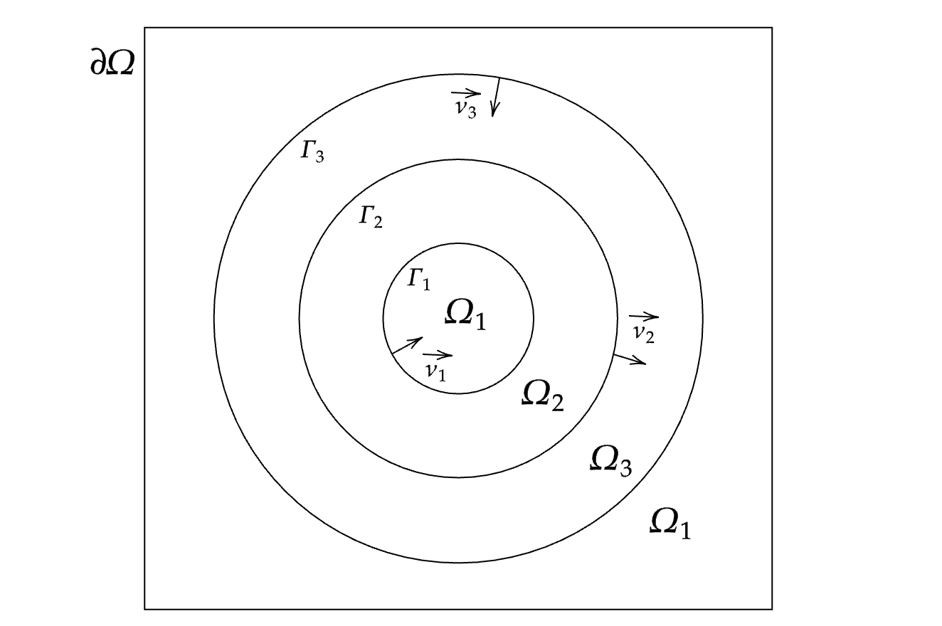
Figure 2: A network of curves which consists of three concentric circles.

We shall prove in Appendix A that $(\mbox{\boldmath{$w$}},\{\Gamma(t)\}_{0\leq t\leq T})$ is a solution to (7.1) with $\sigma=1$ if the three radii satisfy the differential algebraic equations:

$$R^{\prime}_{2}(t)=-F(R_{2}(t)),\quad R_{1}(t)=\sqrt{R_{2}(t)^{2}-A_{2}},\quad R_{3}(t)=\sqrt{R_{2}(t)^{2}+A_{3}},$$ (8.1a)

where $$F(u):=(\frac{1}{\sqrt{u^{2}-A_{2}}}+\frac{1}{u}+\frac{1}{\sqrt{u^{2}+A_{3}}})/({u\log{\frac{u^{2}+A_{3}}{u^{2}-A_{2}}}}) u\in(\sqrt{A_{2}},\infty) A_{2}:=R_{2}(0)^{2}-R_{1}(0)^{2} A_{3}:=R_{3}(0)^{2}-R_{2}(0)^{2}$$ for , , and , and if the three chemical potentials are given by

$$w_{1}(x,\cdot) =-\frac{1}{3R_{2}}-\frac{2}{3R_{3}}+\begin{cases}\frac{1}{3}\alpha\log{\frac{R_{3}^{4}}{R_{1}^{3}R_{2}}},&|x|\leq R_{1}\\ -\frac{1}{3}\alpha\log{\frac{R_{2}|x|^{3}}{R_{3}^{4}}},&R_{1}<|x|\leq R_{3}\\ \frac{1}{3}\alpha\log{\frac{R_{3}}{R_{2}}},&R_{3}<|x|,\end{cases}$$

$$w_{2}(x,\cdot) =\begin{cases}-\frac{1}{R_{1}}-\frac{1}{3R_{2}}-\frac{2}{3R_{3}}+\frac{1}{3}\alpha\log{\frac{R_{3}^{4}}{R_{1}^{3}R_{2}}},&|x|\leq R_{1}\\ -\frac{1}{R_{1}}-\frac{1}{3R_{2}}-\frac{2}{3R_{3}}+\frac{1}{3}\alpha\log{\frac{R_{3}^{4}|x|^{3}}{R_{1}^{6}R_{2}}},&R_{1}<|x|\leq R_{2}\\ \frac{2}{3R_{2}}+\frac{1}{3R_{3}}+\frac{1}{3}\alpha\log{\frac{R_{2}^{2}}{R_{3}^{2}}},&R_{2}<|x|,\end{cases}$$

$$w_{3}(x,\cdot) =\begin{cases}-\frac{1}{R_{1}}-\frac{4}{3R_{2}}-\frac{2}{3R_{3}}+\frac{1}{3}\alpha\log{\frac{R_{2}^{2}R_{3}^{4}}{R_{1}^{6}}},&|x|<R_{2}\\ -\frac{1}{3R_{2}}+\frac{1}{3R_{3}}+\frac{1}{3}\alpha\log{\frac{|x|^{3}}{R_{2}R_{3}^{2}}},&R_{2}\leq|x|<R_{3}\\ -\frac{1}{3R_{2}}+\frac{1}{3R_{3}}+\frac{1}{3}\alpha\log{\frac{R_{3}}{R_{2}}},&R_{3}\leq|x|,\end{cases}$$ (8.1b)

where $\alpha(t):=\frac{\frac{1}{R_{1}{(t)}}+\frac{1}{R_{2}{(t)}}+\frac{1}{R_{3}{(t)}}}{2\log{\frac{R_{3}{(t)}}{R_{1}{(t)}}}}$.

In order to accurately compute the radius $R_{2}(t)$, rather than numerically solving the ODE in (8.1a), we employ a root finding algorithm for the equation

$$0=t+\int_{R_{2}(0)}^{R_{2}(t)}\frac{1}{F(u)}\,du,$$ (8.2)

following similar ideas in [7, 32].

For the initial radii $R_{1}(0)=2$, $R_{2}(0)=2.5$, $R_{3}(0)=3$ and the time interval $[0,T]$ with $T=\frac{1}{2}$, so that $R_{1}(T)\approx 1.60$, $R_{2}(t)\approx 2.20$ and $R_{3}(T)\approx 2.75$, we perform a convergence experiment for the true solution (8.1). To this end, for $i=0\to 4$, we set $N_{f}=\frac{1}{2}K=2^{7+i}$, $N_{c}=4^{i}$ and $\tau=4^{3-i}\times 10^{-3}$. In Table 1 we display the errors

$$\|\Gamma^{h}-\Gamma\|_{L^{\infty}}=\max_{m=1,\ldots,M}\max_{i=1,\ldots,3}\max_{j=1,\ldots,N_{i}}\operatorname{dist}(\vec{q}^{m}_{i,j},\Gamma_{i}(t_{m}))$$

and

$$\|\mbox{\boldmath{$W$}}^{h}-\mbox{\boldmath{$w$}}\|_{L^{\infty}}=\max_{m=1,\ldots,M}\max_{i=1,\ldots,3}\|W^{m}_{i}-I^{m}w_{i}(\cdot,t_{m})\|_{L^{\infty}(\Omega)},$$

where $I^{m}:C^{0}(\overline{\Omega})\to S^{m}$ denotes the standard interpolation operator. We also let $K_{\Omega}^{m}$ denote the number of degrees of freedom of $S^{m}$, and define $h^{m}_{\Gamma}=\max_{i=1,\ldots,3}\max_{j=1,\ldots,N_{i}}\sigma^{m}_{i,j}$. As a comparison, we show the same error computations for the linear scheme (7.3) in Table 2. As expected, we observe true volume preservation for the scheme (7.4) in Table 1, up to solver tolerance, while the relative volume loss in Table 2 decreases as $\tau$ becomes smaller. Surprisingly, the two error quantities $\|\Gamma^{h}-\Gamma\|_{L^{\infty}}$ and $\|\mbox{\boldmath{$W$}}^{h}-\mbox{\boldmath{$w$}}\|_{L^{\infty}}$ are generally lower in Table 2 compared to Table 1, although the difference becomes smaller with smaller discretization parameters.

$h_{f}$	$h^{M}_{\Gamma}$	$\|\mbox{\boldmath{$W$}}^{h}-\mbox{\boldmath{$w$}}\|_{L^{\infty}}$	$\|\Gamma^{h}-\Gamma\|_{L^{\infty}}$	$K^{M}_{\Omega}$	$N$	$|v_{\Delta}^{M}|$
6.2500e-02	1.3469e-01	3.8031e-02	1.3628e-02	3605	384	$<10^{-10}$
3.1250e-02	6.7442e-02	1.3442e-02	6.7806e-03	7285	768	$<10^{-10}$
1.5625e-02	3.3744e-02	5.0754e-03	3.4721e-03	14905	1536	$<10^{-10}$
7.8125e-03	1.6878e-02	2.1316e-03	1.7904e-03	30193	3072	$<10^{-10}$
3.9062e-03	8.4404e-03	1.4242e-03	8.8016e-04	72537	6144	$<10^{-10}$

Table 1: Convergence test for (8.1) over the time interval $[0,\frac{1}{2}]$ for the scheme (7.4).

$h_{f}$	$h^{M}_{\Gamma}$	$\|\mbox{\boldmath{$W$}}^{h}-\mbox{\boldmath{$w$}}\|_{L^{\infty}}$	$\|\Gamma^{h}-\Gamma\|_{L^{\infty}}$	$K^{M}_{\Omega}$	$N$	$|v_{\Delta}^{M}|$
6.2500e-02	1.3487e-01	3.4879e-02	4.7230e-03	3633	384	3.8e-02
3.1250e-02	6.7465e-02	1.2459e-02	4.3450e-03	7321	768	9.7e-03
1.5625e-02	3.3747e-02	4.8323e-03	2.8582e-03	14881	1536	2.4e-03
7.8125e-03	1.6878e-02	2.0917e-03	1.6382e-03	30161	3072	6.1e-04
3.9062e-03	8.4405e-03	1.4139e-03	8.4224e-04	72537	6144	1.5e-04

Table 2: Convergence test for (8.1) over the time interval $[0,\frac{1}{2}]$ for the scheme (7.3).

For all the following numerical simulations, we always employ the fully structure-preserving scheme (7.4).

8.2 Isotropic evolutions with equal surface energies

8.2.1 3 phases

In the next set of experiments, we investigate how a standard double bubble and a disk evolve, when one phase is made up of the left bubble, and the other phase is made up of the right bubble and the disk. With the notation from §7.1 we have $I_{C}=4$, $I_{P}=3$, $I_{T}=2$, $(c^{1}_{1},c^{1}_{2},c^{1}_{3})=(c^{2}_{1},c^{2}_{2},c^{2}_{3})=(1,2,3)$ and $\mathcal{O}=\begin{pmatrix}0&-1&1&0\\ 1&0&-1&-1\\ -1&1&0&1\end{pmatrix}$.

The two bubbles of the double bubble enclose an area of about $3.139$ each, while the disk has an initial radius of $\frac{5}{8}$, meaning it initially encloses an area of $\frac{25\pi}{64}\approx 1.227$. During the evolution the disk vanishes, and the right bubble grows correspondingly, see Figure 3. We note that our theoretically framework does not allow for changes of topology, e.g. the vanishing of curves. Hence, in our computations we perform heuristic surgeries whenever a curve becomes too short.

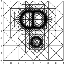
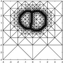
Figure 3: The solution at times $t=0,0.4,0.8,1$, and a plot of the discrete energy over time. Below we show the adaptive bulk mesh at times $t=0$ and $t=1$.

Repeating the simulation with a bigger initial disk gives the results in Figure 4. Here the radius is $\frac{5}{4}$, so that the enclosed area is $4.909$. Now the disk grows at the expense of the right bubble, so that eventually two separate phases remain.

Figure 4: The solution at times $t=0,4,4.5,6$, and a plot of the discrete energy over time.

With the next simulation we demonstrate that in the given setup, which of the two components of phase 1 survives is not down the initial size. In particular, we allow the initial disk to have area $3.300$, so that it is bigger than the other component of the same phase: the right bubble in the double bubble. And yet, due to the perimeter of the bubble being overall cheaper than the boundary of the disk, the latter shrinks to extinction. See Figure 5.

Figure 5: The solution at times $t=0,4,5,7$, and a plot of the discrete energy over time.

For the next experiment we start from a nonstandard triple bubble, where we choose the right most bubble to have area $1.5$, while the other two bubbles have unit area. We assign the two outer bubbles to belong to the same phase. In particular, with the notation from §7.1 we have $I_{C}=6$, $I_{P}=3$, $I_{T}=4$, $(c^{1}_{1},c^{1}_{2},c^{1}_{3})=(1,2,5)$, $(c^{2}_{1},c^{2}_{2},c^{2}_{3})=(1,3,5)$, $(c^{3}_{1},c^{3}_{2},c^{3}_{3})=(2,4,6)$, $(c^{4}_{1},c^{4}_{2},c^{4}_{3})=(3,4,6)$ and

$$\mathcal{O}=\begin{pmatrix}-1&0&0&-1&1&1\\ 0&1&1&0&-1&-1\\ 1&-1&-1&1&0&0\end{pmatrix}.$$

We observe that during the evolution the larger bubble on the right grows at the expense of the left bubble, until the latter one vanishes completely. The remaining interfaces then evolve towards a standard double bubble with enclosed areas 1 and 2.5. See Figure 6.

Figure 6: The solution at times $t=0,0.4,0.6,1$, and a plot of the discrete energy over time.

In the final numerical simulation for the setting with 3 phases, we consider the evolution of two double bubbles. With the notation from §7.1 we have $I_{C}=6$, $I_{P}=3$, $I_{T}=4$, $(c^{1}_{1},c^{1}_{2},c^{1}_{3})=(c^{2}_{1},c^{2}_{2},c^{2}_{3})=(1,2,3)$, $(c^{3}_{1},c^{3}_{2},c^{3}_{3})=(c^{4}_{1},c^{4}_{2},c^{4}_{3})=(4,5,6)$ and

$$\mathcal{O}=\begin{pmatrix}0&-1&1&0&-1&1\\ 1&0&-1&1&0&-1\\ -1&1&0&-1&1&0\end{pmatrix}.$$

The first bubble is chosen with enclosing areas $3.14$ and $6.48$, while the second double bubbles encloses two areas of size $3.64$. In each case, the left bubble is assigned to phase 1, while the right bubbles are assigned to phase 2. In this way, the lower double bubble holds the larger portion of phase 1, while the upper double bubble holds the larger portion of phase 2. Consequently, each double bubble evolves to a single disk that contains just one phase. See Figure 7.

Figure 7: The solution at times $t=0,2,4,5,6,7,8,10,12$, and a plot of the discrete energy over time.

8.2.2 4 phases

In the next set of experiments, we investigate simulations for a nonstandard triple bubble, with one of the bubbles making a phase with a separate disk. In particular, with the notation from §7.1 we have $I_{C}=7$, $I_{P}=4$, $I_{T}=4$, $(c^{1}_{1},c^{1}_{2},c^{1}_{3})=(1,2,5)$, $(c^{2}_{1},c^{2}_{2},c^{2}_{3})=(1,3,5)$, $(c^{3}_{1},c^{3}_{2},c^{3}_{3})=(2,4,6)$, $(c^{4}_{1},c^{4}_{2},c^{4}_{3})=(3,4,6)$ and

$$\mathcal{O}=\begin{pmatrix}0&0&0&-1&0&1&-1\\ 0&1&1&0&-1&-1&0\\ -1&0&0&0&1&0&0\\ 1&-1&-1&1&0&0&1\end{pmatrix}.$$

The three bubbles of the triple bubble enclose an area of unity each, while the disk has an initial radius of $\frac{1}{2}$, meaning it initially encloses an area of $\frac{\pi}{4}\approx 0.785$. During the evolution the disk vanishes, and the right bubble grows correspondingly, see Figure 8.

Figure 8: The solution at times $t=0,0.4,0.7,1$, and a plot of the discrete energy over time.

Repeating the experiment with initial data where the disk is a unit disk leads to the evolution in Figure 9, where the disk now expands and survives, at the expense of the right bubble in the triple bubble.

Figure 9: The solution at times $t=0,0.4,0.8,1$, and a plot of the discrete energy over time.

8.3 Isotropic evolutions with different surface energies

8.3.1 3 phases

As an example for non-equal surface energy densities for the various curves, we repeat the simulation in Figure 3, but now weigh curves 1 and 3 in the double bubble with $\sigma_{1}=\sigma_{3}=2$, while keeping the other two densities at unity. This now means that in contrast to Figure 3, it makes energetically more sense to increase the size of the single bubble, while shrinking the bubble that is surrounded by the more expensive interfaces. See Figure 3 for the observed evolution.

Figure 10: The solution at times $t=0,1,2,3$, and a plot of the discrete energy over time.

8.3.2 4 phases

Similarly, if we make the interface of the single circular bubble in the initial data in Figure 9 more expensive, it will no longer grow but shrink to a point. Setting the weight for the curve to $\sigma_{7}=2$ leads to the evolution seen in Figure 11.

Figure 11: The solution at times $t=0,1,1.8,3$, and a plot of the discrete energy over time.

9 Acknowledgements

A portion of this study was conducted during the research stay of the first author in Regensburg, Germany. He is grateful to the administration of the University of Regensburg for the invitation and for the financial support by the DFG Research Training Group 2339 IntComSin - Project-ID 32182185. He also appreciates the kindness and treatment received from all members in Research Training Group 2339.

Appendix A An exact solution for the three-phase Mullins-Sekerka flow

In this appendix, we shall prove that (8.1) is a solution to (7.1) with $\sigma=1$. Firstly, it directly follows from the definitions of $F$ and $\alpha$ in (8.1) that $F(R_{2}(t))=\alpha(t)/R_{2}(t)$. Hence, (8.1a) immediately implies that the normal velocity $V$ of $\Gamma(t)$ satisfies

$$V=\alpha(t)\begin{cases}\frac{1}{R_{1}(t)}&\mbox{on}\ \ \Gamma_{1}(t),\\ -\frac{1}{R_{2}(t)}&\mbox{on}\ \ \Gamma_{2}(t),\\ \frac{1}{R_{3}(t)}&\mbox{on}\ \ \Gamma_{3}(t).\end{cases}$$ (A.1)

The first and fourth equations in $\eqref{eq:StrongForm_Multi}$ hold trivially since $w$ as defined in (8.1) is constant in the two connected components of $\Omega_{1}(t)$, and harmonic in $\Omega_{2}(t)$ and $\Omega_{3}(t)$. Let us confirm the Gibbs-Thomson law. We see from (8.1) that $w_{1}-w_{2}=1/R_{1}(t)$ on $\Gamma_{1}(t)$, $w_{3}-w_{2}=-1/R_{2}(t)$ on $\Gamma_{2}(t)$ and $w_{3}-w_{1}=1/R_{3}(t)$ on $\Gamma_{3}(t)$. Thus, $w$ satisfies the second condition in $\eqref{eq:StrongForm_Multi}$. We move on the motion law. A direct calculation shows

$$\begin{cases}-\left[{\nabla w_{1}}\right]\cdot\vec{\nu}_{1}=\left[{\nabla w_{2}}\right]\cdot\vec{\nu}_{1}=\frac{\alpha(t)}{R_{1}(t)}\ \ \mbox{on}\ \ \Gamma_{1}(t),\\ \left[{\nabla w_{2}}\right]\cdot\vec{\nu}_{2}=-\left[{\nabla w_{3}}\right]\cdot\vec{\nu}_{2}=-\frac{\alpha(t)}{R_{2}(t)}\ \ \mbox{on}\ \ \Gamma_{2}(t),\\ -\left[{\nabla w_{1}}\right]\cdot\vec{\nu}_{3}=\left[{\nabla w_{3}}\right]\cdot\vec{\nu}_{3}=\frac{\alpha(t)}{R_{3}(t)}\ \ \mbox{on}\ \ \Gamma_{3}(t).\end{cases}$$ (A.2)

Hence, the third condition of $\eqref{eq:StrongForm_Multi}$ is valid by $\eqref{eq:3circleVelocityFormula}$ and $\eqref{eq:3circleVelocityValidation}$. Therefore, $\mbox{\boldmath{$w$}}=(w_{1},w_{2},w_{3})^{T}$ given by $\eqref{eq:ODE}$ is an exact solution of $\eqref{eq:StrongForm_Multi}$ with $\sigma=1$.

References

• [1] W. Bao, H. Garcke, R. Nürnberg, and Q. Zhao, A structure-preserving finite element approximation of surface diffusion for curve networks and surface clusters, Numer. Methods Partial Differ. Eq., 39 (2023), p. 759–794.
• [2] J. W. Barrett and J. F. Blowey, An error bound for the finite element approximation of the Cahn-Hilliard equation with logarithmic free energy, Numer. Math., 72 (1995), pp. 1–20.
• [3] J. W. Barrett, J. F. Blowey, and H. Garcke, Finite element approximation of the Cahn-Hilliard equation with degenerate mobility, SIAM J. Numer. Anal., 37 (1999), pp. 286–318.
• [4]  , On fully practical finite element approximations of degenerate Cahn-Hilliard systems, M2AN Math. Model. Numer. Anal., 35 (2001), pp. 713–748.
• [5] J. W. Barrett, H. Garcke, and R. Nürnberg, On the variational approximation of combined second and fourth order geometric evolution equations, SIAM J. Sci. Comput., 29 (2007), p. 1006–1041.
• [6] J. W. Barrett, H. Garcke, and R. Nürnberg, A parametric finite element method for fourth order geometric evolution equations, J. Comput. Phys., 222 (2007), pp. 441––462.
• [7] J. W. Barrett, H. Garcke, and R. Nürnberg, On stable parametric finite element methods for the Stefan problem and the Mullins-Sekerka problem with applications to dendritic growth, J. Comput. Phys., 229 (2010), p. 6270–6299.
• [8]  , Parametric finite element approximations of curvature-driven interface evolutions, Handb. Numer. Anal., 21 (2020), p. 275–423.
• [9] P. W. Bates and S. Brown, A numerical scheme for the Mullins-Sekerka evolution in three space dimensions, in Differential equations and computational simulations (Chengdu, 1999), World Sci. Publ., River Edge, NJ, 2000, pp. 12–26.
• [10] P. W. Bates, X. Chen, and X. Deng, A numerical scheme for the two phase Mullins-Sekerka problem, Electron. J. Differential Equations, 1995 (1995), pp. 1–27.
• [11] J. F. Blowey, M. I. M. Copetti, and C. M. Elliott, Numerical analysis of a model for phase separation of a multi-component alloy, IMA J. Numer. Anal., 16 (1996), pp. 111–139.
• [12] J. F. Blowey and C. M. Elliott, The Cahn-Hilliard gradient theory for phase separation with nonsmooth free energy. II. Numerical analysis, European J. Appl. Math., 3 (1992), pp. 147–179.
• [13] L. Bronsard, H. Garcke, and B. Stoth, A multi-phase Mullins-Sekerka system: matched asymptotic expansions and an implicit time discretisation for the geometric evolution problem, Proc. Roy. Soc. Edinburgh Sect. A, 128 (1998), p. 481–506.
• [14] C. Chen, C. Kublik, and R. Tsai, An implicit boundary integral method for interfaces evolving by Mullins-Sekerka dynamics, in Mathematics for nonlinear phenomena—analysis and computation, vol. 215 of Springer Proc. Math. Stat., Springer, Cham, 2017, pp. 1–21.
• [15] S. Chen, B. Merriman, S. Osher, and P. Smereka, A simple level set method for solving Stefan problems, J. Comput. Phys., 135 (1997), pp. 8–29.
• [16] X. Chen, J. Hong, and F. Yi, Existence, uniqueness, and regularity of classical solutions of the Mullins-Sekerka problem, Comm. Partial Differential Equations, 21 (1996), pp. 1705–1727.
• [17] T. A. Davis, Algorithm 915, SuiteSparseQR: Multifrontal multithreaded rank-revealing sparse QR factorization, ACM Trans. Math. Software, 38 (2011), pp. 1–22.
• [18] C. M. Elliott and D. A. French, Numerical studies of the Cahn-Hilliard equation for phase separation, IMA J. Appl. Math., 38 (1987), pp. 97–128.
• [19] J. Escher and G. Simonett, Classical solutions for Hele-Shaw models with surface tension, Adv. Differential Equations, 2 (1997), pp. 619–642.
• [20] T. Eto, A rapid numerical method for the Mullins-Sekerka flow with application to contact angle problems, arXiv:2202.13261, (2023).
• [21] D. J. Eyre, Systems of Cahn-Hilliard equations, SIAM J. Appl. Math., 53 (1993), pp. 1686–1712.
• [22] X. Feng and A. Prohl, Error analysis of a mixed finite element method for the Cahn-Hilliard equation, Numer. Math., 99 (2004), pp. 47–84.
• [23]  , Numerical analysis of the Cahn-Hilliard equation and approximation of the Hele-Shaw problem, Interfaces Free Bound., 7 (2005), p. 1–28.
• [24] H. Garcke and M. Rauchecker, Stability analysis for stationary solutions of the Mullins-Sekerka flow with boundary contact, Math. Nachr., 295 (2022), pp. 683–705.
• [25] H. Garcke and T. Sturzenhecker, The degenerate multi-phase Stefan problem with Gibbs-Thomson law, Adv. Math. Sci. Appl., 8 (1998), pp. 929–941.
• [26] S. Hensel and K. Stinson, Weak solutions of Mullins-Sekerka flow as a Hilbert space gradient flow, arXiv:2206.08246, (2022).
• [27] Y. Li, J. Choi, and J. Kim, Multi-component Cahn-Hilliard system with different boundary conditions in complex domains, J. Comput. Phys., 323 (2016), pp. 1–16.
• [28] Y. Li, R. Liu, Q. Xia, C. He, and Z. Li, First- and second-order unconditionally stable direct discretization methods for multi-component Cahn-Hilliard system on surfaces, J. Comput. Appl. Math., 401 (2022), p. 113778.
• [29] S. Luckhaus and T. Sturzenhecker, Implicit time discretization for the mean curvature flow equation, Calculus of Variations and Partial Differential Equations, 3 (1995), p. 253–271.
• [30] U. F. Mayer, A numerical scheme for moving boundary problems that are gradient flows for the area functional., European J. Appl. Math., 11 (2000), p. 61–80.
• [31] R. Nürnberg, Numerical simulations of immiscible fluid clusters, Appl. Numer. Math., 59 (2009), pp. 1612–1628.
• [32]  , A structure preserving front tracking finite element method for the Mullins–Sekerka problem, J. Numer. Math., 31 (2023), pp. 137–155.
• [33] M. Röger, Existence of weak solutions for the Mullins-Sekerka flow, SIAM J. Math. Anal., 37 (2005), pp. 291–301.
• [34] A. Schmidt and K. G. Siebert, Design of Adaptive Finite Element Software: The Finite Element Toolbox ALBERTA, vol. 42 of Lecture Notes in Computational Science and Engineering, Springer-Verlag, Berlin, 2005.
• [35] S. Serfaty, Gamma-convergence of gradient flows on Hilbert and metric spaces and applications, Discrete Contin. Dyn. Syst., 31 (2011), p. 1427–1451.
• [36] J. Zhu, X. Chen, and T. Y. Hou, An efficient boundary integral method for the Mullins–Sekerka problem., J. Comput. Phys., 127 (1996), p. 246–267.