Is It Really Useful to Jointly Parse Constituency and Dependency Trees?
A Revisit

Abstract

This work visits the topic of jointly parsing constituency and dependency trees, i.e., to produce compatible constituency and dependency trees simultaneously for input sentences, which is attractive considering that the two types of trees are complementary in representing syntax. Compared with previous works, we make progress in four aspects: (1) adopting a much more efficient decoding algorithm, (2) exploring joint modeling at the training phase, instead of only at the inference phase, (3) proposing high-order scoring components for constituent-dependency interaction, (4) gaining more insights via in-depth experiments and analysis.

1 Introduction

(a) Constituency tree

[arc angle=80] [row sep=0.2cm, column sep=0.1cm] $ & Logic₁ & plays₂ & a₃ & maximal₄ & role₅ & here₆

[edge style=black!70, thick, edge height=2ex]32nsubj [edge style=black!70, thick, edge height=5ex]13root [edge start x offset=2pt, edge style=black!70, thick, edge height=3ex]64det [edge style=black!70, thick, edge height=1ex]65amod [edge start x offset=1pt, edge end x offset=1pt, edge style=black!70, thick, edge height=6ex]36iobj [edge start x offset=-1pt, edge style=black!70, thick, edge height=9ex]37dobj

(b) Dependency tree

Figure 1: Constituency and dependency trees.

As the most fundamental and long-standing NLP task, syntactic parsing aims to reveal how sentences are syntactically structured. Among many paradigms for representing syntax, constituency trees (c-trees) and dependency trees (d-trees) are the most popular and have gained tremendous research attention in both data annotation and parsing techniques. Figure 1 gives example trees.

As is well known, c-trees and d-trees capture syntactic structure from different yet complementary perspectives Abeillé (2003). On the one hand, c-trees can clearly illustrate how sentences are composed hierarchically. Constituents, especially major phrases like NPs and VPs, are often self-evident and thus easily agreed upon by people. On the other hand, d-trees emphasize on pairwise syntactic (sometimes even semantic) relationship between tokens, i.e., what role (function) the modifier token plays for the head token. It is usually more simple and flexible to draw dependency links than to add constituent nodes.

Therefore, it can be an attractive and useful feature if a parsing model outputs both c-trees and d-trees at the same time. Of course the two trees must be compatible with each other. Basically, compatibility means that for any constituent, only the single head token can compose dependency links, either inwards or outwards, with tokens outside the constituent. Please note that this work and previous works consider only conventional continuous c-trees and projective d-trees.

From the modeling perspective, parsing techniques have achieved immense progress, thanks to the development of deep learning techniques, especially of the pre-trained language models (PLMs) Peters et al. (2018); Devlin et al. (2019). One amazing characteristic is that constituency parsing and dependency parsing have a nearly identical model architecture nowadays. Under the graph-based parsing framework, besides the encoder, the scoring components are the same as well if we treat a constituent as a link between the beginning token and the end token Zhang et al. (2020b). The only difference lies in the decoding algorithms for finding optimal constituency or dependency trees. To some extent, such development stimulates research on joint constituency and dependency parsing (Zhou and Zhao, 2019).

In this work, we revisit Zhou and Zhao (2019) and endeavor to answer the question: is it really useful to jointly parse c- and d-trees? The usefulness is mainly reflected on overall parsing performance. The original work of Zhou and Zhao (2019) performs joint parsing only at the decoding phase. First, they use a lexicalized c-tree to encode both c- and d-trees simultaneously, in which each constituent is annotated with its head token (Collins, 2003). Figure 2 gives an example. They feel the connection between lexicalized trees and head-driven phrase structure grammar (HPSG) Pollard and Sag (1994), and thus call them HPSG trees. Then, they design an ad-hoc decoding algorithm of $O(n^{5})$ time complexity for finding optimal lexicalized c-trees. Under the multi-task learning (MTL) framework, they use one shared encoder, and two separate decoders for the two parsing tasks respectively. Therefore, there is no explicit interaction between the two types of parse trees. Compared with Zhou and Zhao (2019), this work advances this research topic in the following aspects.

1. Inspired by the recent work of Lou et al. (2022) on nested named entity recognition (NER), we employ the Eisner-Satta algorithm of $O(n^{4})$ time complexity for finding optimal lexicalized c-trees (Eisner and Satta, 1999). which runs very efficiently on GPUs after proper batchification Zhang et al. (2020a).

2. Thanks to much improved decoding efficiency, we explore joint modeling at the training phase as well. Moreover, we propose second-order scoring components that allow interaction between constituents and dependencies.

3. We conduct experiments on both English and Chinese benchmark datasets, under settings that are fairer and more easily replicated. Abundant analyses and results are presented to answer our questions and gain insights.

2 Related Work

Before the deep learning era, there exist three competitive families of constituency parsing approaches, i.e., lexicalized PCFG parsing Collins (1999), unlexicalized PCFG parsing Petrov et al. (2006), and discriminative shift-reduce parsing Zhu et al. (2013). Due to the importance of head word features, all three families are more or less related with our work, in the sense that the parser may output d-trees as byproduct at the inference phase.

Lexicalized PCFG parsers generate a c-tree in a head-centered, top-down manner Collins (1999). The head token of each constituent is settled when parsing is finished. Therefore, it is straightforward to acquire unlabeled d-trees.

The unlexicalized parser of Klein and Manning (2003) splits each constituent labels into multiple sub-labels according to linguistic heuristics. For N-ary production rules, they markovize out from the head child, making it feasible to recover unlabeled d-trees likewise.

The discriminative shift-reduce parser of Crabbé (2015) makes heavy use of head tokens for composing features, and therefore is also capable of producing unlabeled d-trees.

Our work is also closely related with Klein and Manning (2002), who factorize a lexicalized c-tree into an unlexicalized c-tree and a d-tree, corresponding to two generative models that are separately trained. They propose an efficient yet inexact A* algorithm for finding the optimal lexicalized c-tree, instead of using the Eisner-Satta (Eisner and Satta, 1999) algorithm.

In the deep learning era, besides Zhou and Zhao (2019), there exist two works that tackle constituency parsing and dependency parsing simultaneously. Strzyz et al. (2019) transform both constituency parsing and dependency parsing into sequence labeling tasks. Fernández-González and Gómez-Rodríguez (2022) transform constituency parsing into a dependency parsing task. During training, both works employ the MTL framework, hence blocking explicit interaction between two sub-modules. More importantly, both works do not consider the compatibility of output c-trees and d-trees at the inference stage.

3 Lexicalized Tree Representation

Given an input sentence $\boldsymbol{x}=w_{1}\dots w_{n}$, we use $\{(i,j,l),0\leq i,j\leq n\}$ as a general denotation of a c-tree $\boldsymbol{c}$ or a d-tree $\boldsymbol{d}$. For a c-tree, $(i,j,l)$ denotes a constituent spanning $w_{i}\dots w_{j}$ and labeled as $l\in\mathcal{L}^{c}$, while for a d-tree, $(i,j,l)$ denotes a dependency from the head word $w_{i}$ to the modifier word $w_{j}$ and labeled as $l\in\mathcal{L}^{d}$.

It is a natural way to encode both a c-tree and a d-tree into a lexicalized tree as the joint representation Collins (2003). Figure 2 gives examples. We convert the original c-tree into Chomsky norm form (CNF), as shown in Figure 2(a), which is required by the graph-based parsing model adopted in this work. Figure 2(b) presents the corresponding lexicalized tree, in which the head tokens are decided by the c-tree in Figure 1(b).

Formally, we denote a lexicalized tree as $\boldsymbol{y}=\{(i,j,h,l)\}$, where $(i,j,h,l)$ represents a lexicalized constituent spanning $w_{i}\dots w_{j}$ with a head word $w_{h}(i\leq h\leq j)$ and a label $l\in\mathcal{L}^{c}$. In the following, we interchangeably use $\mathrm{NP[role]_{3,5}}$ as a simplified notation of $(3,5,5,\mathrm{NP})$.

(a) An unlexicalized c-tree (head-binarized)

(b) An lexicalized c-tree

Figure 2: Example c-trees. The head word of each lexicalized constituent is marked by $\left[\cdot\right]$.

Head-binarization.

As shown earlier, given a c-tree $\boldsymbol{c}$ and a c-tree $\boldsymbol{d}$, we first convert $\boldsymbol{c}$ into CNF before constructing a lexicalized tree $\boldsymbol{y}$, which is required by the CKY algorithm. Of course we assume $\boldsymbol{c}$ and $\boldsymbol{d}$ are compatible with each other before the CNF conversion. The meaning of compatibility is discussed in Section 1.

To avoid incompatibility after CNF conversion, we adopt the head-binarization strategy (Collins, 2003), instead of left- or right-binarization. Basically, head-binarization dynamically selects left- or right-binarization to comply with a given dependency tree. For example, the constituent $\mathrm{VP[plays]}_{2,6}$ in Figure 2(b) is left-binaried, whereas $\mathrm{NP[role]}_{3,5}$ is right-binarized.

Recovering constituency/dependency trees.

It is obvious that a lexicalized tree becomes a constituency tree when discarding the head tokens. Meanwhile, since lexicalized trees are strictly binarized, we can construct the corresponding dependency trees according to the head tokens.

Moreover, please note that dependency labels are not encoded in a lexicalized tree $\boldsymbol{y}$, and are handled via a separate labeling step (see Section 4.2), which is now common practice in parsing models Zhang et al. (2020a).

4 The Joint Parsing Approach

In this section, we introduce how to decompose the score of a lexicalized tree, how to find the optimal tree, and how to define the training loss.

4.1 First-order Factorization

Given $\boldsymbol{y}=(\boldsymbol{c},\boldsymbol{d})$, a naive and simple way is to factorize the score of $\boldsymbol{y}$ as the score sum of $\boldsymbol{c}$ and $\boldsymbol{d}$, without interaction between the two types of trees.

In this way, we define the first-order score of a lexicalized tree as follows.

$${s}(\boldsymbol{x},\boldsymbol{y})=\sum_{(i,j,l)\in\boldsymbol{c}}{s}^{c}(i,j,l)+\sum_{(i,j,l)\in\boldsymbol{d}}{s}^{d}(i,j,l)$$ (1)

where $s^{c/d}(i,j,l)$ is the score of a labeled constituent and a labeled dependency, respectively.

4.2 Two-stage Parsing

Following Dozat and Manning (2017) and Zhang et al. (2020b), we adopt the two-stage parsing strategy, which has been proven to be able to simplify the model architecture and improve efficiency, without hurting performance.

Stage I: Bracketing.

Given $\boldsymbol{x}$, the goal of the first stage is to find an optimal unlabeled lexicalized tree $\boldsymbol{y}$, whose score is:

$$s(\boldsymbol{x},\boldsymbol{y})=\sum_{(i,j)\in\boldsymbol{c}}s^{c}(i,j)+\sum_{i\rightarrow j\in\boldsymbol{d}}s^{d}(i,j)$$ (2)

where $s^{c/d}(i,j)$ denote the scores of unlabeled constituents and unlabeled dependencies, respectively.

Given all $s^{c}(i,j)$ and $s^{d}(i,j)$, the decoding algorithm determines the 1-best lexicalized tree.

$$\hat{\boldsymbol{y}}=\mathop{\mathrm{arg\ max}}\limits_{\boldsymbol{y}\in\mathcal{Y}(\boldsymbol{x})}{s}(\boldsymbol{x},\boldsymbol{y})$$ (3)

where $\mathcal{Y}(\boldsymbol{x})$ denotes the set of all legal lexicalized trees for $\boldsymbol{x}$.

Stage II: Labeling.

Given unlabeled constituents/dependencies in $\hat{\boldsymbol{y}}$ obtained in the first stage, this stage independently predicts labels for them.

$$\hat{l}_{d}=\mathop{\mathrm{arg\ max}}\limits_{l\in\mathcal{L}^{d}}s^{d}(i,j,l)$$ (4)

$$\hat{l}_{c}=\mathop{\mathrm{arg\ max}}\limits_{l\in\mathcal{L}^{c}}s^{c}(i,j,l)$$ (5)

4.3 Training Loss

Given a training instance $(\boldsymbol{x},\boldsymbol{y},\boldsymbol{l})$, the training loss consists of two parts, corresponding to the two stages.

$$L(\boldsymbol{x},\boldsymbol{y},\boldsymbol{l})=L^{\mathrm{bracket}}(\boldsymbol{x},\boldsymbol{y})+L^{\mathrm{label}}(\boldsymbol{x},\boldsymbol{y},\boldsymbol{l}).$$ (6)

For the first part, we adopt the max-margin loss (Taskar et al., 2004), which is based on the margin between the scores of the gold-standard lexicalized tree $\boldsymbol{y}$ and the predicted one $\hat{\boldsymbol{y}}$.

$$\begin{split}&L^{\mathrm{bracket}}=\\ &\quad\mathrm{max}\left(0,\mathop{\mathrm{max}}\limits_{\boldsymbol{y}\neq\hat{\boldsymbol{y}}}\left(s(\boldsymbol{y})-s(\hat{\boldsymbol{y}})+\Delta(\boldsymbol{y},\hat{\boldsymbol{y}})\right)\right)\end{split}$$ (7)

where $\Delta$ is the Hamming distance, which we set as the number of incorrect dependencies and constituents.

For the second-stage loss, we follow Dozat and Manning (2017) and employ cross-entropy loss, i.e., the sum of classification loss over all dependencies and constituents in the gold-standard lexicalized tree $\boldsymbol{y}$.

To alleviate the impact of sentence length, we divide the loss of a training instance by the number of tokens. Moreover, we tried to balance the loss from the two stages the loss via weighted summation, which however has negligible influence on performance according to our preliminary experiments.

4.4 Inference

Zhou and Zhao (2019) propose a naive CKY-style algorithm in $O(n^{5})$ complexity to the simplified HPSG inference, which is highly time-consuming. For lexicalized trees, Eisner and Satta (1999) propose a relatively fast inference that reduces the complexity to $O(n^{4})$ by merging dependency arcs in advance. In this paper, we adopt the Eisner-Satta algorithm to jointly infer the constituency and dependency trees. The deduction rules (Pereira and Warren, 1983) of the algorithm are illustrated in Figure 3.

To further increase the speed of inference, following Zhang et al. (2020a), we batchify the Eisner-Satta algorithm (as shown in Algorithm 1) to fully utilize GPUs. The key to it is calculating the same-length spans in parallel. Therefore, the time complexity of our algorithm is linear in practice.

Figure 3: Deduction rules for Eisner-Satta algorithm (Eisner and Satta, 1999). The triangle-like span $(i,j,h^{\prime})$ is the span $(i,j)$ with the head word $w_{h^{\prime}}\ (h^{\prime}\in[i,j])$, named as the headed span. The hook-like span $(i,j,h)$ is the span $(i,j)$ headed by a arbitrary word $w_{h^{\prime}}$ and the head of $w_{h^{\prime}}$ is $w_{h}\ (h\notin[i,j])$, named as the hooked span. We show only Left-rules, omitting the symmetric Right-rules as well as initial conditions for brevity.

Algorithm 1 The Eisner-Satta Decoding Algorithm.

1:  define: $\alpha,\beta\in\mathbb{R}^{n\times n\times n\times B}$ $\rhd$ $B$ is #sents in a batch

2:  initialize: all $\alpha^{:,:,:}=0$, $\beta^{:,:,:}=0$

3:  for $w=1$ to $n$ do $\rhd$ span width

4:     Batchify: $0\leq i,j=i+w\leq n,r,h$

5:     $\alpha^{i,j,:}=s^{c}(i,j)+\mathop{\mathrm{max}}\limits_{i\leq r<j}\left(\alpha^{i,r,:}+\beta^{r+1,j,:},\beta^{i,r,:}+\alpha^{r+1,j,:}\right)$ $\rhd$ add $s(i,j,:)$ to $\alpha/\beta$ for the 2rd-order expansion

6:     $\beta^{i,j,:}=\mathop{\mathrm{max}}\limits_{i\leq h\leq j}\left(\alpha^{i,j,h}+s^{d}(:,h)\right)$

7:  end for

8:  return  $\alpha^{0,n-1,0}$

4.5 Second-order Extension

In order to further bridge the constituent and dependency trees for deeply joint modeling, we extend the lexicalized tree to the second-order case. From another point of view, the lexicalized constituency tree can be represented as a collection of headed spans and hooked spans (as shown in Figure 3). Hence we further incorporate headed spans and hooked spans scores into the basic first-order model:

$$s^{2o}(\boldsymbol{y})=s(\boldsymbol{y})+\sum_{(i,j,h)\in\boldsymbol{y}}s(i,j,h)$$ (8)

where $s(i,j,h)\in\mathbb{R}^{n\times n\times n}$. If a span $(i,j,h)\in\boldsymbol{y}$ satisfies $h\in[i,j]$, it is shown to be a headed span, and conversely if satisfying $h\notin[i,j]$, it is indicated to be a hooked span.

Besides, we also try to extend other higher-order features, e.g., a structure that combines an arc and a span, and use Mean Field Variational Inference (MFVI). But none of them has performance gains.

5 Model Architecture

In this section, we introduce how to compute scores of lexicalized subtrees.

Encoding.

Given a sentence $\boldsymbol{x}=w_{0},\dots,w_{n+1}$, where $w_{0}$ and $w_{n+1}$ denote the <bos> (begin of a sentence) and <eos> (end of a sentence) tokens respectively, the corresponding hidden representations $\mathbf{e}$ can be obtained via a contextual encoder.

$$\dots,e_{i},\dots=\mathrm{Encoder}(\left[\dots,w_{i},\dots\right])$$ (9)

In this work, we adopt two alternative encoders, i.e., LSTM-based and BERT-based. For the LSTM-based encoder, the word embedding and CharLSTM word representation (Lample et al., 2016) are concatenated as the input vector. Then we feed it into the 3-layer BiLSTMs (Gal and Ghahramani, 2016) to get the contextualized representations $\mathbf{e}$.

For the BERT-based encoder, a sentence is directly fed into BERT encoder (Devlin et al., 2019) to obtain $\mathbf{e}$, without cascading word embedding and LSTM layers for simplicity.

Scoring.

We employ the same scoring functions as Zhang et al. (2020a, b) to compute arc scores $s^{d}(i,j)$ and span scores $s^{c}(i,j)$.

$$r^{\mathrm{head/mod}}_{i}=\mathrm{MLP}^{\mathrm{head/mod}}(\overrightarrow{e_{i}}\oplus\overleftarrow{e_{i}})$$ (10)

$$r^{\mathrm{left/right}}_{i}=\mathrm{MLP}^{\mathrm{left/right}}(\overrightarrow{e_{i}}\oplus\overleftarrow{e_{i+1}})$$ (11)

$$s^{d}(i,j)=\begin{bmatrix}r_{j}^{\mathrm{mod}}\oplus 1\end{bmatrix}^{\mathrm{T}}\mathbf{W}^{d}r_{i}^{\mathrm{head}}$$ (12)

$$s^{c}(i,j)=\begin{bmatrix}r_{i}^{\mathrm{left}}\oplus 1\end{bmatrix}^{\mathrm{T}}\mathbf{W}^{c}r_{j}^{\mathrm{right}}$$ (13)

where MLPs are applied to obtain lower $k$-dimensional vectors; $r^{\mathrm{head/mod}}_{i}$ are the representation vectors of $w_{i}$ as a head/modifier respectively, and analogously, $r^{\mathrm{left/right}}_{i}$ are the left/right boundary representation of $w_{i}$; $\overrightarrow{e_{i}}/\overleftarrow{e_{i}}$ are hidden representations of $w_{i}$ in different contextual orientations. $\mathbf{W}^{d/c}\in\mathbb{R}^{(k+1)\times k}$ are trainable parameters.

For second-order features, we adopt the same scoring functions as Yang and Tu (2022b) to calculate headed spans and hooked spans:

$$r^{\mathrm{word}}_{i}=\mathrm{MLP}^{\mathrm{word}}(\overrightarrow{e_{i}}\oplus\overleftarrow{e_{i}})$$ (14)

$$h^{\mathrm{span}}_{i,j}=\left[\overrightarrow{e_{i}}\oplus\overleftarrow{e_{i+1}}\right]-\left[\overrightarrow{e_{j}}\oplus\overleftarrow{e_{j+1}}\right]$$ (15)

$$r^{\mathrm{span}}_{i,j}=\mathrm{MLP}^{\mathrm{span}}(h^{\mathrm{span}}_{i,j})$$ (16)

$$s(i,j,h)=\begin{bmatrix}r_{h}^{\mathrm{word}}\oplus 1\end{bmatrix}^{\mathrm{T}}\mathbf{W}^{\mathrm{span}}\begin{bmatrix}r_{i,j}^{\mathrm{span}}\oplus 1\end{bmatrix}$$ (17)

where $\mathbf{W}^{\mathrm{span}}\in\mathbb{R}^{(k+1)\times(k+1)}$.

According to the two-stage strategy, it is similar to calculating dependency and constituency labels scores, referring Zhang et al. (2020a, b) for details.

6 Experiments

Data.

We conduct experiments on English Penn Treebank (PTB) (Marcus et al., 1993) and Chinese Treebank (CTB5.1) (Xue et al., 2005), which are widely used in the community. Following Zhou and Zhao (2019), we use the Stanford Dependencies conversion software of version 3.3 and Penn2Malt to obtain the corresponding dependency trees. For CTB5.1, we adopt the split from Zhang and Clark (2008), which is commonly used for dependency parsing. We do not use the split from Zhu et al. (2013) because the test set was too small, containing just over three hundred sentences. More details on data splits are given in Table 1.

	Train	Dev	Test
PTB	39,832	1,700	2,416
CTB5	16,091	803	1,910

Table 1: Data statistics on sentence numbers.

Evaluation metrics.

For dependency parsing, we adopt unlabeled and labeled attachment scores (UAS/LAS) as metrics. For constituency parsing, we adopt the standard constituent-level labeled precision (P), recall (R), and F1-score as metrics. Consistent with Zhou and Zhao (2019), we omit all punctuation for dependency parsing.

Models.

Joint1o and Joint2o both perform joint modeling but with the first/second-order score separately. To facilitate a comprehensive comparison, we introduce three additional models: Dep, Con, and Mtl. Dep/Con are essentially the same dependency and constituency parsing models as Zhang et al. (2020a, b), except that we apply the max-margin loss to unify the loss function. Mtl, just as the name implies, employs multi-task learning (MTL) framework to perform the constituency and dependency parsing. We adopt the max-margin loss for each parsing task and sum them up as MTL loss. By default, Mtl adopts head-binarization and joint decoding. All models use the same parameters.

Settings and parameters.

For the LSTM-based models, we utilize Glove embeddings for English, and adopt the embeddings trained on Gigaword 3rd Edition for Chinese following Li et al. (2019). For the BERT-based models, we employ Bert-Large-Cased for English and Bert-Base-Chinese for Chinese. We directly adopt the same hyper-parameters of the parser from Zhang et al. (2020a, b). For the second-order model, we set the dimensions of $r^{\mathrm{word}}_{i}/r^{\mathrm{span}}_{i,j}$ to 100. We note that reporting the results of using gold Part-Of-Speech (POS) tags for Chinese is a more prevalent practice (Zhou and Zhao, 2019; Mohammadshahi and Henderson, 2021; Fernández-González and Gómez-Rodríguez, 2022). Therefore, for comprehensive comparisons, we also conduct experiments with gold POS tags. For the LSTM-based models, we concatenate POS tag embeddings (100d) with word embeddings. For the BERT-based models, POS tag embeddings are added element-wise to the hidden representations from the encoder. We report results averaged over 3 runs with different random seeds for all experiments.

	PTB					CTB5
	LAS	F1	Inc. Trees	Inc. Const.		LAS	F1	Inc. Trees	Inc. Const.
Dep	94.03	-	23.31	01.69		87.47	-	44.08	03.54
Con	-	94.33				-	87.72
Mtl w/o joint decode	94.14	94.18	12.51	01.71		87.80	87.63	26.32	02.68
Mtl	94.15	94.31	00.00	00.00		87.86	87.76	00.00	00.00
Joint1o	94.20	94.24	00.00	00.00		87.90	87.60	00.00	00.00
Joint2o	94.26	94.25	00.00	00.00		87.99	87.62	00.00	00.00
	+BERT
Dep	94.80	-	14.63	01.80		90.52	-	32.54	03.23
Con	-	95.78				-	90.81
Mtl w/o joint decode	94.86	95.68	05.37	01.46		90.63	90.78	20.22	02.37
Mtl	94.87	95.71	00.00	00.00		90.69	90.86	00.00	00.00
Joint1o	94.89	95.72	00.00	00.00		90.70	90.70	00.00	00.00
Joint2o	94.92	95.75	00.00	00.00		90.76	90.74	00.00	00.00

Table 2: Model study on dev data. “Inc.Trees” measures the percentage of incompatible c- and d-trees in the parsing results, and “Inc.Const.” further measures the number of incompatible constituents included in each incompatible c-tree on average.

6.1 Main Results

Comparison on LAS and F1.

Table 2 presents the results of our model study on dev data. We observe that for the LSTM-based models, the joint parsing models (including Mtl, Joint1o and Joint2o) all showed absolute performance gains compared to Dep, especially Joint2o, which achieves an improvement of 0.23 LAS on PTB test and 0.52 LAS on CTB5 test.

For constituency parsing, however, joint parsing models do not lead to a steady improvement. We believe it is probably because the relevance of dependency parsing and constituency parsing is inherently high, i.e., the dependency treebanks are transformed through the constituency treebanks based on head-finding rules. Consequently, the only external information available to the constituency parser is the head-finding rules, which may limit the potential for significant performance gains.

Regarding joint constituency and dependency parsing, we observe that their performances are generally similar, and our Joint1o model slightly outperforms Mtl in dependency parsing but lags behind in constituency parsing. Additionally, there is a minor yet consistent performance gain of Joint2o over Joint1o in all cases, confirming the effectiveness of our incorporation of second-order features in the modeling process.

Compatibility.

We introduce two additional metrics, namely, incompatible trees and incompatible constituents, to assess the compatibility (discussed in Section 1) of parsed c- and d-trees. Specifically, constituents are considered incompatible with dependencies either if they have multiple head tokens, or if outward dependency arcs start from non-head tokens. Such cases result in incompatible c-trees and d-trees. From these two metrics, we find that despite using head-binarization during training, Mtl still parses incompatible results without joint decoding, where 12.51% of the parsed results on PTB are incompatible, with each incompatible result containing an average of 1.71 incompatible constituents. Meanwhile, not using joint decoding also results in a small performance drop. Further, we align the parsing results of $\textsc{Dep}/\textsc{Con}$ and find that the percentage of incompatible results is higher than Mtl. These results show the significance of head-binarization and joint decoding in joint parsing.

The above findings hold consistently across experiments with BERT as well, but the gaps between the different models become smaller due to the strong representational capabilities of the pre-trained models.

	Dependency		Constituency
	UAS	LAS	P	R	F1
Zhang+20a†	96.14	94.49	-	-	-
Zhang+20b†	-	-	94.23	94.02	94.12
M&H21†	96.44	94.71	-	-	-
HPSG19	96.09	94.68	93.92	93.64	93.78
F&G22	96.25	94.64	-	-	93.67
Joint2o	96.32	94.69	94.30	94.13	94.22
	+BERT
M&H21†	96.66	95.01	-	-	-
Y&T22†	-	-	96.19	95.83	96.01
HPSG19	97.00	95.43	95.98	95.70	95.84
F&G22	96.97	95.46	-	-	95.23
Joint2o	97.11	95.57	96.15	95.59	95.87

Table 3: Comparison with previous results on PTB-test. HPSG19: Zhou and Zhao (2019). Zhang+20a: Zhang et al. (2020a). Zhang+20b: Zhang et al. (2020b). M&H21: Mohammadshahi and Henderson (2021). F&G22: Fernández-González and Gómez-Rodríguez (2022). Y&T22: Yang and Tu (2022a). ^† indicates using only the constituency or dependency treebank.

	Dependency		Constituency
	UAS	LAS	P	R	F1
Zhang+20a†	88.77	87.25	-	-	-
Zhang+20b†	-	-	87.35	87.78	87.57
Joint2o	89.32	87.87	87.48	87.82	87.65
	w/ gold POS tags
M&H21†	91.85	90.12	-	-	-
HPSG19	91.21	89.15	91.16	90.91	91.03
Joint2o	91.88	91.51	91.47	91.63	91.55
	+BERT
M&H21†	92.98	91.18	-	-	-
Joint2o	93.34	92.94	93.04	93.19	93.11

Table 4: Comparison with previous results on CTB5-test. HPSG19: Zhou and Zhao (2019). Zhang+20a: Zhang et al. (2020a). Zhang+20b: Zhang et al. (2020b). M&H21: Mohammadshahi and Henderson (2021). F&G22: Fernández-González and Gómez-Rodríguez (2022). ^† indicates using only the constituency or dependency treebank.

6.2 Comparison with Previous Works

Table 3 and 4 compare our Joint2o with the existing state-of-the-art of both the separate and joint parsing on test sets. On PTB, the result of our Joint2o with BERT is 95.57 LAS and 95.87 F1. The performance gap between Joint2o and recent state-of-the-art parsers is negligibly small.

On CTB5, we re-run the code released by Zhang et al. (2020a, b) to reproduce their results. In comparison to Zhang et al. (2020a), our Joint2o model demonstrates a substantial improvement in LAS (0.62) for dependency parsing, while delivering a performance similar to Zhang et al. (2020b) for constituency parsing. Furthermore, when provided with gold POS tags, our model achieves remarkable improvements of 2.36 on LAS and 0.52 on F1 compared to the results reported by Zhou and Zhao (2019) for dependency and constituency parsing, respectively.

6.3 Analysis

In the previous experiments, we only use attachment scores and F1 scores to evaluate the performance of parsing, which assess the accuracy of dependencies and constituents, respectively. However, upon analyzing the results in Table 2, we observed that the differences between the models were relatively small, with gaps of less than 0.5. For more detailed analyses, we evaluate the parsing results from other perspectives.

Complete match of syntactic trees.

To facilitate a more evident comparison between different models, following Zhang et al. (2019), we adopt a more challenging metric known as the sentence-level labeled complete match (LCM). Specifically, we evaluated the LCM of the predicted d-trees, c-trees, and lexicalized trees with the gold ones, denoted as LCM_dep/LCM_con/LCM_lex respectively. Noted that an instance where the LCM_lex is true only if both the LCM_dep and LCM_con are true.

	LCMdep	LCMcon	LCMlex
Dep&Con	40.79	29.21	25.55
Mtl	42.41	29.46	27.38
Joint1o	43.17	28.60	27.68
Joint2o	43.71	29.39	28.27

Table 5: The complete matching on CTB5-test.

Similar to the results of the model study in Table 2, we find that compared to separate parsing model Dep/Con, the joint parsing models have improved performance on matching d-trees, especially Joint2o, and the performances on matching c-trees are all close. Additionally, we also calculated the performance of Dep/Con on matching lexicalized tree and find it significantly lower than the joint models, which demonstrates the advantages of the joint parsing model for parsing lexicalized trees.

Among the joint parsing models, Mtl performs better for the complete matching of c-trees, and Joint1o and Joint2o perform better for the dependency tree. On LCM_lex, Joint1o compared to Mtl does not improve, suggesting that the first-order lexicalized tree modeling based on the dependencies and constituents features does not bring help for the complete matching of the lexicalized tree. In contrast, Joint2o exhibited a substantial improvement of 0.59 compared to Joint1o and 0.89 compared to Mtl on LCM_lex. This finding indicates that the inclusion of the headed/hooked span features unique to the lexicalized tree is effective in improving the complete match performance of the lexicalized tree.

Performance on different constituent widths and dependency lengths.

Yang and Tu (2022b) shows that different tree modelings may influence the performance on different constituent widths and dependency lengths. To investigate this, we follow Yang and Tu (2022b) to plot unlabeled precision/recall as functions of the constituent widths and dependency lengths. The width of a constituent from $w_{i}$ to $w_{j}$ is equal to $d:=|i-j|$. Precision represents the percentage of predicted constituents of width $d$ that are correct. Recall measures the percentage of gold standard constituents of width $d$ that are predicted.

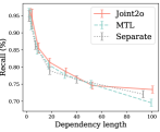
Figure 4: Constitency and dependency parsing under different lengths on CTB5-test.

Figure 4 shows the results under different constituent widths and dependency lengths. Specifically, “Separate” denotes the separate parsing models Dep and Con. We employ adaptive binning (Ding et al., 2020) to mitigate performance fluctuations caused by small sample sizes within each bin to ensure stable and reliable outcomes. The size of each bar corresponds to the number of samples within the bin: larger bars indicate a higher number of samples .

Figure 4 and 4 show the precision/recall for constituents of different constituent widths. Notably, Mtl and separate model Con consistently perform better than Joint2o across almost all widths on precision. However, when we focus on Figure 4, an interesting observation emerges: our joint modeling method exhibits higher recall for wide constituents (width $>$ 40). This finding indicates that our joint modeling approach is particularly effective in recalling wide constituents.

From Figure 4 and 4, we can see that for short dependencies (of length $\leq$ 50), all three models perform comparably. However, for long dependencies (length $>$ 50), our Joint2o model exhibits the best performance on both precision and recall. This demonstrates the advantage of our joint modeling in parsing long-range dependencies.

7 Conclusions

This paper revisits the work of Zhou and Zhao (2019) and try to find out whether it is useful to jointly parse c- and d-trees. Compared with Zhou and Zhao (2019), we further explore joint modeling at the training phase, thanks to the improved efficiency from the Eisner-Satta Eisner and Satta (1999) decoding algorithm. We also design second-order scoring components for promoting interaction between constituents and dependencies. We conduct experiments on both English and Chinese datasets. Results and further analysis lead to the following findings.

First, compared with separate modeling, joint modeling consistently improves dependency parsing performance, yet constituency parsing performance changes little, or even slightly decreases. The trend is clearer on Chinese, probably because the baseline performance on Chinese is much lower than on English.

Second, joint modeling at the training phase and second-order interaction are both helpful, and can improving the complete matching ratio over whole d-trees and lexicalized trees.

Third, joint modeling improves the precision/recall ratio of long-distance dependencies, which contributes to the overall performance improvement for dependency parsing.

Fourth, joint modeling improves the recall ratio of wide constituents, but decreases their precision ratio.

References

- Abeillé (2003) Anne Abeillé. 2003. Introduction. Treebanks: Building and Using Parsed Corpora (editor: Anne Abeillé). Kluwer Academic Publishers.
- Collins (1999) Michael Collins. 1999. Head-driven statistical models for natural language parsing. PhD thesis, University of Pennsylvania.
- Collins (2003) Michael Collins. 2003. Head-driven statistical models for natural language parsing. CL.
- Crabbé (2015) Benoit Crabbé. 2015. Multilingual discriminative lexicalized phrase structure parsing. In Proceedings of EMNLP.
- Devlin et al. (2019) Jacob Devlin, Ming-Wei Chang, Kenton Lee, and Kristina Toutanova. 2019. BERT: Pre-training of deep bidirectional transformers for language understanding. In Proceedings of NAACL-HLT.
- Ding et al. (2020) Yukun Ding, Jinglan Liu, Jinjun Xiong, and Yiyu Shi. 2020. Revisiting the evaluation of uncertainty estimation and its application to explore model complexity-uncertainty trade-off. In Conference on Computer Vision and Pattern Recognition, CVPR Workshops.
- Dozat and Manning (2017) Timothy Dozat and Christopher D. Manning. 2017. Deep biaffine attention for neural dependency parsing. In Proceedings of ICLR.
- Eisner and Satta (1999) Jason Eisner and Giorgio Satta. 1999. Efficient parsing for bilexical context-free grammars and head automaton grammars. In Proceedings of ACL.
- Fernández-González and Gómez-Rodríguez (2022) Daniel Fernández-González and Carlos Gómez-Rodríguez. 2022. Multitask pointer network for multi-representational parsing. Knowledge-Based Systems.
- Gal and Ghahramani (2016) Yarin Gal and Zoubin Ghahramani. 2016. Dropout as a bayesian approximation: Representing model uncertainty in deep learning. In Proceedings of ICML.
- Kitaev and Klein (2018) Nikita Kitaev and Dan Klein. 2018. Constituency parsing with a self-attentive encoder. In Proceedings of ACL.
- Klein and Manning (2002) Dan Klein and Christopher Manning. 2002. Fast exact inference with a factored model for natural language parsing. In Advances in Neural Information Processing Systems.
- Klein and Manning (2003) Dan Klein and Christopher D. Manning. 2003. Accurate unlexicalized parsing. In Proceedings of ACL.
- Lample et al. (2016) Guillaume Lample, Miguel Ballesteros, Sandeep Subramanian, Kazuya Kawakami, and Chris Dyer. 2016. Neural architectures for named entity recognition. In Proceedings of NAACL-HLT.
- Li et al. (2019) Ying Li, Zhenghua Li, Min Zhang, Rui Wang, Sheng Li, and Luo Si. 2019. Self-attentive biaffine dependency parsing. In Proceedings of IJCAI-19.
- Lou et al. (2022) Chao Lou, Songlin Yang, and Kewei Tu. 2022. Nested named entity recognition as latent lexicalized constituency parsing. In Proceedings of ACL.
- Marcus et al. (1993) Mitchell P. Marcus, Beatrice Santorini, and Mary Ann Marcinkiewicz. 1993. Building a large annotated corpus of English: The Penn Treebank. CL.
- Mohammadshahi and Henderson (2021) Alireza Mohammadshahi and James Henderson. 2021. Recursive non-autoregressive graph-to-graph transformer for dependency parsing with iterative refinement. TACL.
- Pereira and Warren (1983) Fernando C. N. Pereira and David H. D. Warren. 1983. Parsing as deduction. In Proceedings of ACL.
- Peters et al. (2018) Matthew E. Peters, Mark Neumann, Mohit Iyyer, Matt Gardner, Christopher Clark, Kenton Lee, and Luke Zettlemoyer. 2018. Deep contextualized word representations. In Proceedings of NAACL.
- Petrov et al. (2006) Slav Petrov, Leon Barrett, Romain Thibaux, and Dan Klein. 2006. Learning accurate, compact, and interpretable tree annotation. In Proceedings of ACL.
- Pollard and Sag (1994) Carl Pollard and Ivan Sag. 1994. Head-driven phrase structure grammar. University of ChicagoPress.
- Strzyz et al. (2019) Michalina Strzyz, David Vilares, and Carlos Gómez-Rodríguez. 2019. Sequence labeling parsing by learning across representations. In Proceedings of ACL.
- Taskar et al. (2004) Ben Taskar, Dan Klein, Mike Collins, Daphne Koller, and Christopher Manning. 2004. Max-margin parsing. In Proceedings of EMNLP.
- Xue et al. (2005) Naiwen Xue, Fei Xia, Fu-Dong Chiou, and Matra Palmer. 2005. The penn chinese treebank: Phrase structure annotation of a large corpus. Nat.Lang.Eng.
- Yang and Tu (2022a) Songlin Yang and Kewei Tu. 2022a. Bottom-up constituency parsing and nested named entity recognition with pointer networks. In Proceedings of ACL.
- Yang and Tu (2022b) Songlin Yang and Kewei Tu. 2022b. Headed-span-based projective dependency parsing. In Proceedings of ACL.
- Zhang et al. (2020a) Yu Zhang, Zhenghua Li, and Zhang Min. 2020a. Efficient second-order TreeCRF for neural dependency parsing. In Proceedings of ACL.
- Zhang et al. (2020b) Yu Zhang, Houquan Zhou, and Zhenghua Li. 2020b. Fast and accurate neural CRF constituency parsing. In Proceedings of IJCAI.
- Zhang and Clark (2008) Yue Zhang and Stephen Clark. 2008. A tale of two parsers: Investigating and combining graph-based and transition-based dependency parsing. In Proceedings of EMNLP.
- Zhang et al. (2019) Zhisong Zhang, Xuezhe Ma, and Eduard Hovy. 2019. An empirical investigation of structured output modeling for graph-based neural dependency parsing. In Proceedings of ACL.
- Zhou and Zhao (2019) Junru Zhou and Hai Zhao. 2019. Head-Driven Phrase Structure Grammar parsing on Penn Treebank. In Proceedings of ACL.
- Zhu et al. (2013) Muhua Zhu, Yue Zhang, Wenliang Chen, Min Zhang, and Jingbo Zhu. 2013. Fast and accurate shift-reduce constituent parsing. In Proceedings of ACL.