On the role of soft gluons in collinear parton densities

DESY-23-172

1 Introduction

Calculations based on the DGLAP [1, 2, 3, 4] evolution of parton densities together with hard scattering coefficient functions (or matrix elements) at next-to-leading (NLO) and next-to-next-to-leading order (NNLO) in the strong coupling provide a very successful description of experimental measurements from small to rather large scales $\mu$.

The Parton-Branching (PB) approach [5, 6] gives a solution to the DGLAP equations, based on an iterative solution of the integral evolution equation. The PB-approach also allows to study in detail each of the branching vertices, and in particular the contribution of perturbative and non-perturbative emissions. In the frame of Transverse Momentum Dependent (TMD) parton densities [7, 8] and especially in the CSS formalism [9], a non-perturbative Sudakov form factor is introduced, in addition. In the PB-approach this non-perturbative Sudakov form factor already appears in inclusive (collinear) parton densities, and with the determination of collinear parton densities by fits to inclusive experimental data, the non-perturbative Sudakov form factor is fixed also when applied to TMD parton densities.

In this paper we show explicitly how the Sudakov from factor is obtained from the DGLAP evolution equation and how this form factor can be split into a perturbative and non-perturbative part. We argue, that both parts are essential for collinear parton distributions, as neglecting soft gluons would lead to non-cancellation of singular contribution in cross section calculations at NLO and beyond.

2 PB approach as a solution of DGLAP

The PB method [5, 6] provides a solution of the DGLAP [1, 2, 3, 4] evolution equations. The DGLAP evolution equation for the parton density of parton $a$ with momentum fraction $x$ at the scale $\mu$ reads:

$$\mu^{2}\frac{{\partial}{f}_{a}(x,\mu^{2})}{{\partial}\mu^{2}}=\sum_{b}\int_{x}^{1}{\frac{dz}{z}}\;{P}_{ab}\left(\alpha_{s}(\mu^{2}),z\right)\;{f}_{b}\left({\frac{x}{z}},\mu^{2}\right)\;,$$ (1)

with the regularized DGLAP splitting functions $P_{ab}$ describing the splitting of parton $b$ into a parton $a$. The splitting functions $P_{ab}$ can be decomposed as (in the notation of Ref. [5]):

$${P}_{ab}(z,\alpha_{s})=D_{ab}(\alpha_{s})\delta(1-z)+K_{ab}(\alpha_{s})\frac{1}{(1-z)_{+}}+R_{ab}(z,\alpha_{s})\;.$$ (2)

The coefficients $D$ and $K$ can be written as $D_{ab}(\alpha_{s})=\delta_{ab}d_{a}(\alpha_{s})$, $K_{ab}(\alpha_{s})=\delta_{ab}k_{a}(\alpha_{s})$ and the coefficients $R_{ab}$ contain only terms which are not singular for $z\rightarrow 1$. Each of those three coefficients can be expanded in powers of $\alpha_{s}$:

$$d_{a}(\alpha_{s})=\sum_{n=1}^{\infty}\left(\frac{\alpha_{s}}{2\pi}\right)^{n}d_{a}^{(n-1)},\;k_{a}(\alpha_{s})=\sum_{n=1}^{\infty}\left(\frac{\alpha_{s}}{2\pi}\right)^{n}k_{a}^{(n-1)},\;R_{ab}(z,\alpha_{s})=\sum_{n=1}^{\infty}\left(\frac{\alpha_{s}}{2\pi}\right)^{n}R_{ab}^{(n-1)}(z)$$ (3)

The plus-prescription and the $D$ part in eq.(2) can be expanded and eq.(1) can be reformulated introducing a Sudakov form factor $\Delta^{S}_{a}(\mu^{2})$ (for details on the calculation see the appendix Sec. 6) which is defined as:

$$\Delta^{S}_{a}(\mu^{2},\mu^{2}_{0})=\exp\left(-\int_{\mu_{0}^{2}}^{\mu^{2}}\frac{\textrm{d}\mu^{\prime 2}}{\mu^{\prime 2}}\left[\int_{0}^{z_{M}}k_{a}(\alpha_{s})\frac{1}{1-z}\textrm{d}z-d_{a}(\alpha_{s})\right]\right)\;,$$ (4)

where an upper limit $z_{M}=1-\epsilon\;$ is introduced to allow numerical integration over $z$. In order to reproduce DGLAP, $\epsilon\to 0$ is required. Note, that the expression of $\Delta^{S}_{a}$ is different from the one used in Ref. [5], for a relation of both see the appendix Sec. 6. The evolution equation for the parton density ${f}_{a}(x,\mu^{2})$ at scale $\mu$ is then given by (as a solution of eq.(1), see also [10]):

$${f}_{a}(x,\mu^{2})=\Delta^{S}_{a}(\mu^{2})\ {f}_{a}(x,\mu^{2}_{0})+\sum_{b}\int^{\mu^{2}}_{\mu^{2}_{0}}{{d\mu^{\prime 2}}\over\mu^{\prime 2}}{{\Delta^{S}_{a}(\mu^{2})}\over{\Delta^{S}_{a}(\mu^{\prime 2})}}\int_{x}^{z_{M}}{\frac{dz}{z}}\;\hat{P}_{ab}(\alpha_{s}(\mu^{\prime 2}),z)\;{f}_{b}\left({\frac{x}{z}},\mu^{\prime 2}\right)$$ (5)

with the unregularized splitting functions $\hat{P}_{ab}$ (without the $D_{ab}$ piece, replacing $1/(1-z)_{+}$ by $1/(1-z)$) and $\mu_{0}$ being the starting scale. Since the evolution equation is solved iteratively, one has access to every individual branching vertex, and thus one can calculate also the transverse momenta ($q_{\rm t}$) of the emitted partons. Details on the formulation for TMD parton distributions are given in Ref. [5]).

On a collinear level, it was shown in Ref. [5] that the PB  approach reproduces exactly the DGLAP evolution of parton densities [11], if the renormalization scale (the argument in $\alpha_{s}$) is set to the evolution scale $\mu$ and if $z_{M}\to 1$. In Ref. [12] the PB parton distributions are obtained from a fit [13, 14] of the parameters of the $x$-dependent starting distributions to describe high-precision deep-inelastic scattering data [15]. Two different parton distribution sets (we use PB-NLO-2018 as a shorthand notation for PB-NLO-HERAI+II-2018) were obtained, PB-NLO-2018 Set1, which for collinear distributions agrees exactly with HERAPDF2.0NLO [15], and another set, PB-NLO-2018 Set2, which uses $q_{\rm t}$ as the argument in $\alpha_{s}$, inspired by angular ordering conditions. All PB  parton distributions (and many others) are accessible in TMDlib and via the graphical interface TMDplotter [16, 17].

In the following, we concentrate on the PB-NLO-2018 Set1 scenario because of its direct correspondence to standard DGLAP solutions, a discussion on PB-NLO-2018 Set2 is given in Ref. [18, 19].

2.1 The PB Sudakov form factor

The concept of resolvable and non-resolvable branchings with Sudakov form factors allows for an intuitive interpretation of the parton evolution pattern. The Sudakov form factors give the probability to evolve from one scale to another scale without resolvable branching. While the concept of the PB method is similar to a parton shower approach, the method is used here to solve the DGLAP evolution equation.

In order to illustrate the importance of resolvable and non-resolvable branchings we separate the Sudakov form factor $\Delta^{S}_{a}$ into a perturbative ($q_{\rm t}>q_{0}$) and non-perturbative ($q_{\rm t}<q_{0}$) part by introducing a resolution scale $z_{\rm dyn}=1-q_{0}/q$ (see Ref. [20]). This scale is motivated by angular ordering and the requirement to resolve an emitted parton with $q_{\rm t}=q(1-z)>q_{0}$.

The Sudakov form factor is then given by :

$$\Delta_{a}^{S}(\mu^{2},\mu^{2}_{0})= \exp\left(-\int^{\mu^{2}}_{\mu^{2}_{0}}{{dq^{2}}\over q^{2}}\left[\int_{0}^{z_{\rm dyn}(q)}dz\frac{k_{a}(\alpha_{s})}{1-z}-d_{a}(\alpha_{s})\right]\right)$$ (6)

$$\times\exp\left(-\int^{\mu^{2}}_{\mu^{2}_{0}}{{dq^{2}}\over q^{2}}\int_{z_{\rm dyn}(q)}^{z_{M}}dz\frac{k_{a}(\alpha_{s})}{1-z}\right)$$

$$= \Delta_{a}^{(\text{P})}\left(\mu^{2},\mu_{0}^{2},q^{2}_{0}\right)\cdot\Delta_{a}^{(\text{NP})}\left(\mu^{2},\mu_{0}^{2},\epsilon,q_{0}^{2}\right)\;.$$

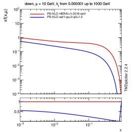
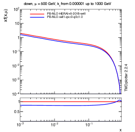
Figure 1: Integrated down-quark distributions at $\mu=10,100$ GeV and $\mu=500$ GeV obtained from the PB approach for different values of $z_{M}$: PB-NLO-HERAI+II-set1 applies $z_{M}\to 1$ and PB-NLO-set1 applies $z_{M}=z_{\rm dyn}$ with $q_{0}=1$ GeV and without intrinsic -$k_{\rm T}$ distribution ($q_{s}=0$). The ratio plots show the ratios to the one for $z_{M}\to 1$.

It is interesting to note, that $\Delta_{a}^{(\text{NP})}$ develops a $\log\mu$ dependence, and under certain conditions, $\Delta_{a}^{(\text{NP})}$ can be even calculated analytically. It is this $\log\mu$ dependence which makes the non-perturbative contribution of soft gluon emissions and the resulting net transverse momentum so different from any intrinsic $k_{\rm T}$-dependence, which is $\mu$-scale independent.

In Fig. 1 we show parton distributions obtained with the PB approach using the starting distributions from PB-NLO-2018 Set1 from Ref. [12] for different scales $\mu$. We show distributions for down quark parton densities for different values of $z_{M}$: $z_{M}\to 1$ (default) and $z_{M}=z_{\rm dyn}=1-q_{0}/q$, with $q_{0}=1$ GeV and without any intrinsic $k_{\rm T}$-distribution ($q_{s}=0$), which by definition does not matter for the integrated parton densities. The distributions obtained from PB-NLO-2018 set1 with $z_{M}\to 1$ are significantly different from those applying $z_{M}=z_{\rm dyn}$, illustrating the importance of soft contributions even for collinear distributions. Comparing the collinear distributions at low and high scales $\mu$, a clear scale dependence of the contribution on soft gluons (and $\Delta_{a}^{(\text{NP})}$) is observed.

It is obvious that limiting the $z$-integration by $z_{\rm dyn}$ (and neglecting $\Delta_{a}^{(\text{NP})}$) leads to distributions which are no longer consistent with the collinear $\overline{\rm MS}$ factorization scheme. A similar conclusion was found in Ref. [23].

Since the PB-approach can also be used to determine TMD parton distributions (see Ref. [5]) we will illustrate in Fig. 2 the effect of the $z_{M}$ cut-off in the transverse momentum distribution. We show results obtained with the PB-approach for down quarks for PB-NLO-2018 Set1 with a default Gaussian width $q_{s}=0.5$ GeV for the intrinsic $k_{\rm T}$-distribution. Since we want to focus only on the evolution (as given in eq.(6)), we show also the results when no intrinsic $k_{\rm T}$-distribution is applied ($q_{s}=0$ GeV, practically we use a Gauss distribution with $q_{s}=0.0001$ GeV) and we illustrate the effect of neglecting $\Delta_{a}^{(\text{NP})}$ (by applying $z_{\rm dyn}=1-q_{0}/q$, as in Fig. 1).

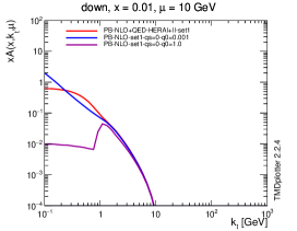
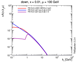
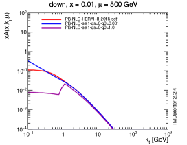
Figure 2: Transverse momentum distributions of down quarks at $\mu=10,100$ GeV (left, middle column) and $\mu=500$ GeV (right column) obtained from the PB approach for $z_{M}\to 1$ as well as $z_{M}=z_{\rm dyn}=1-q_{0}/q$. The red curve shows PB-NLO-2018 Set1 (including intrinsic-$k_{\rm T}$), the blue curve shows a prediction without including any intrinsic-$k_{\rm T}$ distribution ($q_{s}=0$), and the magenta curve shows a prediction applying $z_{M}=z_{\rm dyn}$ with $q_{0}=1.0$ GeV without including intrinsic-$k_{\rm T}$ distributions.

The transverse momentum distributions show very clearly the effect of $\Delta_{a}^{(\text{NP})}$. Applying the cutoff-scale, $z_{M}=z_{\rm dyn}=1-q_{0}/q$, removes emissions with $q_{\rm t}<q_{0}$ (there are still low-$k_{\rm T}$ contributions, which come from adding vectorially all intermediate emissions). However, very soft emissions are automatically included with $z_{M}\to 1$. Please note, that if $\alpha_{s}(q_{\rm t})$ is chosen a special treatment is needed for $q_{\rm t}<q_{0}$.

As seen in Figs. 1,2 the contribution of soft gluons is $\mu$-scale dependent. Assuming that any intrinsic transverse motion of partons inside hadrons is universal ($\mu$-scale independent), soft gluon emission cannot be mimicked by any intrinsic-$k_{\rm T}$ distribution, but rather the soft gluon contribution needs to be properly resummed.

3 Cross Section calculation

Physical cross sections are calculated as a convolution of the scale dependent parton densities with the hard matrix elements (coefficient functions). For simplicity, we show only the calculation of deep inelastic scattering with NLO parton densities and coefficient functions, the expressions are given in text books (i.e. Ref. [10] eq. 4.80 ):

$$F_{2}(x,Q^{2})=x\sum_{q,\bar{q}}e_{q}^{2}\int_{x}^{1}\frac{d\xi}{\xi}q(\xi,Q^{2})\left[\delta\left(1-\frac{x}{\xi}\right)+\frac{\alpha_{s}}{2\pi}C_{\over{\rm MS}}\left(\frac{x}{\xi}\right)+\cdots\right]$$ (7)

with the coefficient function $C_{\over{\rm MS}}$ in $\overline{\rm MS}$-scheme. The $\overline{\rm MS}$ coefficient function for massless quarks at ${\cal O}(\alpha_{s})$ read:

$$C^{\over{\rm MS}}_{q}(z) = C_{F}\left[2\left(\frac{\log(1-z)}{1-z}\right)_{+}-\frac{3}{2}\left(\frac{1}{1-z}\right)_{+}-(1+z)\log(1-z)\right.$$ (8)

$$\left.-\frac{1+z^{2}}{1-z}\log z+3+2z-\left(\frac{\pi^{2}}{3}+\frac{9}{2}\right)\delta(1-z)\right]$$

For a consistent formulation, the integral over $\xi$ in eq.(7) has to extend up to one, both in the expression for the cross section, as well as in the expression for the parton density, otherwise singular pieces remain un-cancelled.

It becomes clear, that the contribution of soft gluon emissions is important both in the parton densities as well as in the cross section calculations. Approaches, where the integral is limited by $z_{\rm dyn}$ lead to a different factorization scheme and the coefficient functions obtained in collinear, massless $\overline{\rm MS}$-scheme are no longer appropriate. In Ref. [24] the same issue is discussed from the perspective of Monte Carlo event generators and the use of collinear parton densities in a backward evolution approach for the parton shower.

From the above considerations, we can summarize, that the region of soft gluon emissions is very important in the evolution of the parton densities, as well as in the calculation of the hard cross section. Within the PB-approach, the non-perturbative Sudakov form factor is constrained by the fit to inclusive measurements to determine inclusive parton distributions: once the evolution frame is specified (depending on the scale choice for $\alpha_{s}$), the non-perturbative Sudakov form factor is fixed by the fit to inclusive measurements. The PB-TMD distributions are then calculated without any further assumptions.

4 Implications from soft gluon emissions

The treatment of soft gluon emissions will lead also to effects in different physics processes: soft gluons are very important for the description of the low $p_{\rm T}$-region in Drell-Yan production and different effects can be expected in particle (jet) spectra coming from initial state parton showers.

4.1 Drell-Yan $p_{\rm T}$-spectrum

The Drell-Yan $p_{\rm T}$-spectrum at large transverse moment is described by hard single parton emissions, at lower $p_{\rm T}$ soft gluons have to be resummed. Also the intrinsic motion of parton inside the hadrons plays a role. In Ref. [25] the Drell Yan $p_{\rm T}$-spectrum at low and high Drell-Yan masses and at different center-of-mass energies is discussed, and it is found that PB-NLO-2018 Set2 leads to a rather reasonable description. In Ref. [18, 19] a very detailed analysis of the description of the Drell-Yan transverse momentum spectrum is given, with the result that after a determination of the parameter $q_{s}$ of the intrinsic $k_{\rm T}$-distribution, PB-NLO-2018 Set2 leads to a very good description of Drell-Yan measurements at different Drell-Yan masses $m_{\small\text{DY}}$ and as well at different center-of-mass energies $\sqrt{s}$. The success of describing the DY $p_{\rm T}$-spectrum with PB-NLO-2018 Set2 is ascribed to the inclusion of $\Delta_{a}^{(\text{NP})}$ and the treatment of $\alpha_{s}$ at small scales.

This can be contrasted to the behaviour of standard parton shower Monte Carlo event generator based on collinear parton densities which need an intrinsic-$k_{\rm T}$ spectrum dependent on $\sqrt{s}$. In Ref. [26] a study is reported on tuning the parameter of the intrinsic $k_{\rm T}$-distribution for the Monte Carlo event generators, Pythia and Herwig (with the most recent tunes). It is found that the gaussian width $q_{s}$ of the intrinsic $k_{\rm T}$-distribution depends on $\sqrt{s}$ (for both generators and differnt tunes).

4.2 Soft gluon emissions in parton shower Monte Carlo event generators

In Monte Carlo event generators, the initial parton shower is generated in a backward evolution approach for efficiency reasons (see e.g. Refs. [27, 28, 29, 30, 31, 32]). In event generators based on collinear parton densities, the accumulated transverse momentum of the initial state cascades determine the total transverse momentum of the hard process, e.g. in Drell-Yan production the initial state radiation determines the Drell-Yan $p_{\rm T}$. In Monte Carlo generators based on TMD distributions (e.q. Cascade3 [32]), the transverse momentum of the hard process is already determined by the TMD distribution, and the initial state parton shower is not allowed to change this, rather only adding radiated partons. Such a treatment allows to study the effect of a different $z_{\rm dyn}$-values in the initial state shower, without changing the overall kinematics. We use Drell-Yan production at NLO (simulated by MadGraph5_aMC@NLO) supplemented with TMD distributions and initial state parton shower from Cascade3, as described in Refs [33, 34, 25, 35].

We first investigate (Fig. 3) the spectrum of the splitting variable $z$ and the rapidity $y$ of emitted partons in the initial state shower for different values of $q_{0}$ leading to different values of $z_{\rm dyn}=1-q_{0}/q$. Since $z_{\rm dyn}$ depends on $q$ and very different values of $q=q_{\rm t}/(1-z)$ are accessible in the evolution, no clear cut in $z_{\rm dyn}$ is observed, however, the spectrum itself depends significantly on $z_{\rm dyn}$ and $q_{0}$.

Figure 3: Distributions of the splitting variable $z$ (left) and the rapidity of emitted partons $y$ (right) during the initial state shower for different values of $q_{0}$ in $Z$-boson events.

Next, we investigate the transverse momentum spectrum of emitted partons in the initial state shower for different values of $q_{0}$. In Fig. 4(left) we show the transverse momentum ($q_{\rm t}$) spectrum of all partons emitted in the initial state shower for different values of $q_{0}$.

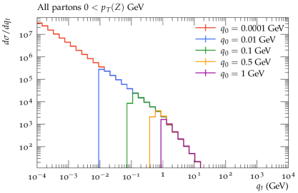
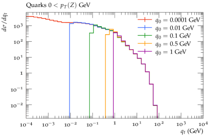
Figure 4: Transverse momentum distributions of emitted partons in the initial state cascade for different values of $q_{0}$ in $Z$-boson events. In (left) is shown the spectrum for all partons, in (right) is shown the spectrum for quarks only.

It is evident that extremely low values of $q_{0}$ result in a significant number of very soft (non-perturbative) emissions. In Fig. 4(right) we show the same distributions but only for emitted quarks. As expected, for such processes $g\to q\bar{q}$ and $q\to gq$ there is no singular behavior of the splitting function for $z\to 1$ and the spectrum at low transverse momenta is rather flat, compared to the one, where gluon emission is included.

It is interesting to investigate whether these soft gluons change any of the observable hadron distributions. In the Lund string hadronization [36, 37, 38, 39] gluons are treated as kinks in the color strings, therefore very soft gluons are expected to have a negligible effect. In Fig. 5 we show the spectra the transverse momentum and rapidity of particles in $Z$-boson events. The small dependence on $q_{0}$ seen in the rapidity spectrum comes from very low $p_{\rm T}$-hadrons. While the spectrum of partons is very different for different values of $q_{0}$, there is essentially no effect on $q_{0}$ visible in the particle spectra, leading to stable final results.

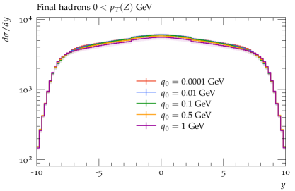
Figure 5: Transverse momentum (left) and rapidity (right) distributions of particles for different values of $q_{0}$. The bump at large $p_{\rm T}$ comes from the muons of the $Z$-boson decay.

In summary we observe, that the effect of different $z_{\rm dyn}$-values in the corresponding non-perturbative Sudakov form factor $\Delta_{a}^{(\text{NP})}$ is rather significant for the low $p_{\rm T}$-spectrum of partons in the initial state cascade (and therefore important for the Drell-Yan $p_{\rm T}$), while the effect is negligible for final state hadron spectra and even more for jets coming from the initial state shower.

5 Summary and Conclusion

We have investigated the perturbative and non-perturbative regions of collinear parton densities, by making use of the formulation of the DGLAP evolution equation in terms of Sudakov form factors applied in the PB-method. The separation of the Sudakov form factor into a perturbative and non-perturbative part is motived by investigations of the Drell-Yan transverse momentum spectrum within the CSS approach.

We find, that soft (non-perturbative) gluon emissions play a significant role in inclusive parton distributions, and those emissions are an essential part of the $\overline{\rm MS}$-scheme: neglecting those would lead to non-cancellation of important singular pieces.

With the requirement to describe and fit inclusive distributions, like the inclusive DIS cross-section, the non-perturbative Sudakov form factor is constrained and determined, once the factorization and evolution scheme for collinear parton densities is fixed (i.e. the choice of scale for the evolution of the strong coupling $\alpha_{s}$, which implies also a different form of the non-perturbative Sudakov form factor). The non-perturbative Sudakov form factor, fixed from inclusive distributions, plays an important role in the description of the Drell-Yan transverse momentum spectrum.

We have investigated the effect of soft gluons for the transverse momentum spectrum of emitted partons and hadrons. While soft gluons are essential to describe the complete parton density and the low $p_{\rm T}$-spectrum of, for example, Drell-Yan lepton pairs, the effect of soft gluons on the spectra of produced particles (and jets) is negligible.

6 Appendix: The Sudakov form factor

The DGLAP splitting functions in evolution equation eq.(1) can be written in different forms, where the plus-prescription acts on different terms:

$${P}_{ab}(z,\alpha_{s}) = {P}(z,\alpha_{s})_{+}$$ (9)

$$= D_{ab}(\alpha_{s})\delta(1-z)+K_{ab}(\alpha_{s})\frac{1}{(1-z)_{+}}+R_{ab}(z,\alpha_{s})\;$$ (10)

The plus prescription is given by:

$$\int_{0}^{1}dz\frac{\phi(z)}{(1-z)_{+}} = \int_{0}^{1}dz\frac{\phi(z)-\phi(1)}{(1-z)}$$ (11)

$$= \lim_{\epsilon\to 0}\int_{0}^{1-\epsilon}dz\frac{\phi(z)}{(1-z)}-\lim_{\epsilon\to 0}\int_{0}^{1-\epsilon}dz\frac{\phi(1)}{(1-z)}\;,$$ (12)

where the last line is used for expanding the plus-prescription. Applying eq.(9) and eq.(12) leads to:

$$\mu^{2}\frac{{\partial}{f}_{a}(x,\mu^{2})}{{\partial}\mu^{2}} = \sum_{b}\int_{x}^{1}{\frac{dz}{z}}\;{P}_{ab}\left(z\right)\;{f}_{b}\left({\frac{x}{z}},\mu^{2}\right)$$ (13)

$$= \sum_{b}\int_{0}^{1}\frac{dz}{z}\;P_{ab}\left(z\right)\;f_{b}\left({\frac{x}{z}}\right)-\sum_{b}\int_{0}^{x}\frac{dz}{z}\;P_{ab}(z)\;f_{b}\left(\frac{x}{z}\right)$$ (14)

$$= \sum_{b}\int_{0}^{1}dz\;\hat{P}_{ab}\left(z\right)\left(\frac{1}{z}\;f_{b}\left({\frac{x}{z}}\right)-f_{b}(z)\right)-\sum_{b}\int_{0}^{x}\frac{dz}{z}\;\hat{P}_{ab}\left(z\right)\;f_{b}\left(\frac{x}{z}\right)$$ (15)

$$= \sum_{b}\int_{x}^{1}\frac{dz}{z}\;\hat{P}_{ab}\left(z\right)\;f_{b}\left({\frac{x}{z}}\right)-f_{a}(x)\sum_{b}\int_{0}^{1}dz\;\hat{P}_{ab}\left(z\right)$$ (16)

$$= \sum_{b}\int_{x}^{1}\frac{dz}{z}\;\hat{P}_{ab}\left(z\right)\;f_{b}\left({\frac{x}{z}}\right)+f_{a}(x)\frac{\mu^{2}}{\Delta_{a}}\frac{\partial\Delta_{a}}{\partial\mu^{2}}$$ (17)

where we dropped $\alpha_{s}$ and $\mu^{2}$ dependence for better reading. The unregularized splitting function is denoted by $\hat{P}$ (without the $D_{ab}$ piece, and replacing $1/(1-z)_{+}$ by $1/(1-z)$), and the Sudakov form factor $\Delta_{a}(\mu^{2})$ is given by:

$$\Delta_{a}(\mu^{2})=\exp\left(-\sum_{b}\int_{\mu_{0}^{2}}^{\mu^{2}}\frac{d\mu^{\prime 2}}{\mu^{\prime 2}}\int_{0}^{1-\epsilon}dz\hat{P}_{ab}(\alpha_{s},z)\right)$$ (18)

With this, the evolution equation for ${f_{a}\left(x,\mu^{2}\right)}/{\Delta_{a}(\mu^{2})}$ is given by (see [10]):

$$\mu^{2}\frac{\partial}{\partial\mu^{2}}\frac{f_{a}(x,\mu^{2})}{\Delta_{a}(\mu^{2})}=\sum_{b}\int_{x}^{1}\frac{dz}{z}\;\hat{P}_{ab}\left(z\right)\;\frac{f_{b}\left({\frac{x}{z},\mu^{2}}\right)}{\Delta_{a}(\mu^{2})}$$ (19)

If instead we start from eq.(10), and apply the same steps as above, we obtain:

$$\mu^{2}\frac{{\partial}{f}_{a}(x,\mu^{2})}{{\partial}\mu^{2}} = \sum_{b}\int_{x}^{1}{\frac{dz}{z}}\;{P}_{ab}\left(z\right)\;{f}_{b}\left({\frac{x}{z}},\mu^{2}\right)$$ (20)

$$= \sum_{b}\int_{0}^{1}\frac{dz}{z}\;\left(D_{ab}\delta(1-z)+K_{ab}\frac{1}{(1-z)_{+}}+R_{ab}(z)\right)\;f_{b}\left(\frac{x}{z}\right)$$ (22)

$$= \sum_{b}\int_{0}^{1}\frac{dz}{z}\left(\frac{K_{ab}}{1-z}+R_{ab}(z)\right)f_{b}\left(\frac{x}{z}\right)$$

$$-f_{a}(z)\int_{0}^{1}dz\left(\frac{k_{a}}{(1-z)}-d_{a}\delta(1-z)\right)\;$$

The Sudakov form factor $\Delta_{S}(\mu^{2})$ is now defined as (see eq.(4)):

$$\Delta_{a}^{S}(\mu^{2})=\exp\left(-\int_{\mu_{0}^{2}}^{\mu^{2}}\frac{d\mu^{\prime 2}}{\mu^{\prime 2}}\int_{0}^{1-\epsilon}dz\left[\frac{k_{a}}{(1-z)}-d_{a}\delta(1-z)\right]\right)\;,$$ (24)

leading to an evolution equation for ${f_{a}\left(x,\mu^{2}\right)}/{\Delta^{S}_{a}(\mu^{2})}$.

References

- [1] V. N. Gribov and L. N. Lipatov, “Deep inelastic scattering in perturbation theory”, Sov. J. Nucl. Phys. 15 (1972) 438. [Yad. Fiz.15,781(1972)].
- [2] L. N. Lipatov, “The parton model and perturbation theory”, Sov. J. Nucl. Phys. 20 (1975) 94. [Yad. Fiz.20,181(1974)].
- [3] G. Altarelli and G. Parisi, “Asymptotic freedom in parton language”, Nucl. Phys. B 126 (1977) 298.
- [4] Y. L. Dokshitzer, “Calculation of the structure functions for Deep Inelastic Scattering and annihilation by perturbation theory in Quantum Chromodynamics.”, Sov. Phys. JETP 46 (1977) 641. [Zh. Eksp. Teor. Fiz.73,1216(1977)].
- [5] F. Hautmann et al., “Collinear and TMD quark and gluon densities from Parton Branching solution of QCD evolution equations”, JHEP 01 (2018) 070, arXiv:1708.03279.
- [6] F. Hautmann et al., “Soft-gluon resolution scale in QCD evolution equations”, Phys. Lett. B 772 (2017) 446, arXiv:1704.01757.
- [7] J. Collins and T. C. Rogers, “Connecting Different TMD Factorization Formalisms in QCD”, Phys. Rev. D 96 (2017) 054011, arXiv:1705.07167.
- [8] H. Jung, S. T. Monfared, and T. Wening, “Determination of collinear and TMD photon densities using the Parton Branching method”, Physics Letters B 817 (2021) 136299, arXiv:2102.01494.
- [9] J. C. Collins, D. E. Soper, and G. F. Sterman, “Transverse Momentum Distribution in Drell-Yan Pair and W and Z Boson production”, Nucl. Phys. B 250 (1985) 199.
- [10] R. K. Ellis, W. J. Stirling, and B. R. Webber, “QCD and collider physics”, Camb. Monogr. Part. Phys. Nucl. Phys. Cosmol. 8 (1996) 1.
- [11] M. Botje, “QCDNUM: fast QCD evolution and convolution”, Comput.Phys.Commun. 182 (2011) 490, arXiv:1005.1481.
- [12] A. Bermudez Martinez et al., “Collinear and TMD parton densities from fits to precision DIS measurements in the parton branching method”, Phys. Rev. D 99 (2019) 074008, arXiv:1804.11152.
- [13] xFitter Developers’ Team Collaboration, H. Abdolmaleki et al., “xFitter: An Open Source QCD Analysis Framework. A resource and reference document for the Snowmass study”, 6, 2022. arXiv:2206.12465.
- [14] S. Alekhin et al., “HERAFitter, Open Source QCD Fit Project”, Eur. Phys. J. C 75 (2015) 304, arXiv:1410.4412.
- [15] ZEUS, H1 Collaboration, “Combination of measurements of inclusive deep inelastic scattering cross sections and QCD analysis of HERA data”, Eur. Phys. J. C 75 (2015) 580, arXiv:1506.06042.
- [16] N. A. Abdulov et al., “TMDlib2 and TMDplotter: a platform for 3D hadron structure studies”, Eur. Phys. J. C 81 (2021) 752, arXiv:2103.09741.
- [17] F. Hautmann et al., “TMDlib and TMDplotter: library and plotting tools for transverse-momentum-dependent parton distributions”, Eur. Phys. J. C 74 (2014), no. 12, 3220, arXiv:1408.3015.
- [18] S. Taheri Monfared, “NLO Analysis of Small- Region in Drell-Yan Production with Parton Branching”, 11, 2023. arXiv:2311.04746.
- [19] I. Bubanja et al., “The small - region in Drell-Yan production at next-to-leading order with the Parton Branching Method”. to be published.
- [20] F. Hautmann, L. Keersmaekers, A. Lelek, and A. M. Van Kampen, “Dynamical resolution scale in transverse momentum distributions at the LHC”, Nucl. Phys. B 949 (2019) 114795, arXiv:1908.08524.
- [21] A. M. van Kampen, “Drell-Yan transverse spectra at the LHC: a comparison of parton branching and analytical resummation approaches”, SciPost Phys. Proc. 8 (2022) 151, arXiv:2108.04099.
- [22] A. Bermudez Martinez et al., “The TMD Parton Branching Sudakov Form Factor in the context of TMD factorization”. to be published.
- [23] Z. Nagy and D. E. Soper, “Evolution of parton showers and parton distribution functions”, Phys. Rev. D 102 (2020), no. 1, 014025, arXiv:2002.04125.
- [24] S. Frixione and B. R. Webber, “Correcting for cutoff dependence in backward evolution of QCD parton showers”, arXiv:2309.15587.
- [25] A. Bermudez Martinez et al., “The transverse momentum spectrum of low mass Drell–Yan production at next-to-leading order in the parton branching method”, Eur. Phys. J. C 80 (2020) 598, arXiv:2001.06488.
- [26] S. Taheri Monfared, “Intrinsic Distribution Independence in Drell-Yan Spectra Predictions: A Novel Insight from the Parton-Branching Method”, in Proceedings of the Physics in Collisions. 2023.
- [27] M. Bengtsson, T. Sjostrand, and M. van Zijl, “Initial state radiation effects on W and jet production”, Z. Phys. C 32 (1986) 67.
- [28] T. Sjostrand, “A model for initial state parton showers”, Phys.Lett. B157 (1985) 321.
- [29] G. Marchesini and B. R. Webber, “Monte Carlo Simulation of General Hard Processes with Coherent QCD Radiation”, Nucl. Phys. B 310 (1988) 461.
- [30] B. R. Webber, “Monte Carlo Simulation of Hard Hadronic Processes”, Ann. Rev. Nucl. Part. Sci. 36 (1986) 253.
- [31] G. Marchesini and B. R. Webber, “Simulation of QCD Jets Including Soft Gluon Interference”, Nucl. Phys. B 238 (1984) 1.
- [32] S. Baranov et al., “CASCADE3 A Monte Carlo event generator based on TMDs”, Eur. Phys. J. C 81 (2021) 425, arXiv:2101.10221.
- [33] H. Yang et al., “Back-to-back azimuthal correlations in jet events at high transverse momentum in the TMD parton branching method at next-to-leading order”, Eur. Phys. J. C 82 (2022) 755, arXiv:2204.01528.
- [34] M. I. Abdulhamid et al., “Azimuthal correlations of high transverse momentum jets at next-to-leading order in the parton branching method”, Eur. Phys. J. C 82 (2022) 36, arXiv:2112.10465.
- [35] A. Bermudez Martinez et al., “Production of Z-bosons in the parton branching method”, Phys. Rev. D 100 (2019) 074027, arXiv:1906.00919.
- [36] H.-U. Bengtsson and T. Sjostrand, “The Lund Monte Carlo for hadronic processes: Pythia Version 4.8”, Comput.Phys.Commun. 46 (1987) 43.
- [37] H. Bengtsson and G. Ingelman, “The Lund Monte Carlo for high pt Physics”, Comput.Phys.Commun. 34 (1985) 251.
- [38] T. Sjöstrand, “PYTHIA 5.7 and JETSET 7.4: physics and manual”, arXiv:hep-ph/9508391.
- [39] T. Sjöstrand, S. Mrenna, and P. Skands, “PYTHIA 6.4 physics and manual”, JHEP 05 (2006) 026, arXiv:hep-ph/0603175.