1 Introduction

Wasserstein distance (Earth Mover Distance) [46] has been widely recognized as a geometrically meaningful metric for comparing probability measures. As evidence, Wasserstein distance has been successfully applied to various applications such as generative modeling [49], domain adaptation [10], clustering [22], and so on. Specifically, Wasserstein distance serves as the standard metric for applications involving 3D data, such as point-cloud reconstruction [1], point-cloud registration [51], point-cloud completion [23], point-cloud generation [26], mesh deformation [13], image style transfer [3], and various other tasks.

Despite its appealing performance, Wasserstein distance exhibits high computational complexity. When using conventional linear programming solvers, the evaluation of Wasserstein distance carries a time complexity of $\mathcal{O}(n^{3}\log n)$ [46], particularly when dealing with discrete probability measures containing at most $n$ atoms. Furthermore, the space complexity of computing Wasserstein distance is at least $\mathcal{O}(n^{2})$, which is required for storing the pairwise transportation cost matrix. Sliced Wasserstein (SW) distance [6] stands as a rapid alternative metric to Wasserstein distance. Since SW distance is defined as a sliced probability metric based on Wasserstein distance, it remains equivalent to Wasserstein distance while retaining its appealing properties [36]. More importantly, the time complexity and space complexity of SW are only $\mathcal{O}(n\log n)$ and $\mathcal{O}(n)$, respectively. As a result, SW distance has found successful adoption in various applications, including domain adaptation [31], generative models [37], clustering [28], gradient flows [5], Bayesian inference [56], and more. In the realm of 3D data, SW distance is employed in numerous applications such as point-cloud registration [29], reconstruction, and generation [40], point-cloud upsampling [50], mesh deformation [30], image style transfer [32], texture synthesis [20], along with various other tasks

Formally, SW distance is defined as the expectation of the Wasserstein distance between two one-dimensional projected measures under the uniform distribution over projecting directions, i.e., the unit hypersphere. The computation of SW distance is well-known to be intractable; hence, in practice, it is estimated empirically through Monte Carlo (MC) integration as a replacement. Specifically, (pseudo)-random samples are drawn from the uniform distribution over the unit hypersphere to approximate the integration. However, the approximation error of MC integration is suboptimal because (pseudo)-uniform random samples may not exhibit high uniformity [43]. To address this issue, Quasi-Monte Carlo (QMC) methods [25] are introduced. In greater detail, QMC utilizes points sets known as "low-discrepancy sequences" to approximate the expectation, in contrast to i.i.d. random samples in MC. Since the samples in the points set have low discrepancy, they are more "uniform" and provide a superior approximation of the uniform expectation over the domain.

The conventional QMC method primarily focuses on integration over the unit cube, denoted as $[0,1]^{d}$ (for $d\geq 1$). To assess the uniformity of a points set within the unit cube, the widely employed metric is the "star-discrepancy" [27]. A lower star-discrepancy value typically results in reduced approximation error, as per the Koksma–Hlawka inequality [27]. When a points set exhibits a sufficiently small star-discrepancy, it is referred to as a "low-discrepancy sequence". For the unit cube, several methods exist to construct such low-discrepancy sequences, including the Halton sequence [16], Hammersley points set [17], Faure sequencecitepfaure1982discrepance, Niederreiter sequence[41], and the widely used Sobol sequence [52]. QMC is renowned for its efficiency and effectiveness, particularly in relatively low dimensions, such as 3D applications. However, it is worth noting that SW distance necessitates integration over the unit hypersphere of dimension $d-1$ rather than the unit cube.

Contribution. In summary, our contributions are three-fold:

1. We provide an overview of practical methods for constructing points sets on the unit hypersphere, which can serve as candidates for low-discrepancy sequences (referred to as QMC points sets). Specifically, our exploration encompasses the following techniques: (i) mapping a low-discrepancy sequence from the 3D unit cube to the unit hypersphere using the normalized inverse Gaussian CDF, (ii) transforming a low-discrepancy sequence from the 2D unit grid to the unit hypersphere via Lambert equal-area mapping, (iii) Utilizing generalized spiral points, (iv) maximizing pairwise absolute discrepancy, (v) minimizing the Coulomb energy. Notably, we believe that our work marks the first instance of employing the recent numerical formulation of spherical cap discrepancy [19] to assess the uniformity of the aforementioned points sets.

2. . We introduce Quasi-Sliced Wasserstein (QSW), which comprises a family of deterministic approximations to the sliced Wasserstein distance based on Quasi-Monte Carlo (QMC) points sets. Furthermore, we establish the asymptotic convergence of QSW to SW for nearly all constructions of QMC points sets. For stochastic optimization, we present Randomized Quasi-Monte Carlo (RMQC) methods applied to the unit sphere, resulting in Randomized Quasi-Sliced Wasserstein (RQSW). In particular, we explore two approaches for generating random points sets on $\mathbb{S}^{d-1}$: transforming randomized points sets from the unit cube and random rotation. We provide proof that nearly all variants of RQSW constitute unbiased estimations of SW

3. We empirically demonstrate that QSW and RQSW offer more favorable approximations to SW in 3D applications. To elaborate, we initially establish that QSW provides a superior approximation to population SW compared to conventional Monte Carlo (MC) approximations when comparing 3D empirical measures over point clouds. Furthermore, we conduct experiments involving point-cloud interpolation, image style transfer, and training deep point-cloud autoencoders to showcase the superior performance of various QSW and RQSW variants.

Organization. The remainder of the paper is organized as follows. We first review the background on the SW distance, MC estimation, and QMC in Section 2. Then, we discuss how to construct QMC points sets on $\mathbb{S}^{d-1}$, define QSW and RQSW, and discuss some theoretical properties in Section 3. Section 4 contains experiments on point-cloud autoencoder, image style transfer, and deep point-cloud reconstruction. We conclude the paper in Section 5. Finally, we defer the proofs of key results, related works, and additional materials to the Appendices.

Notations. For any $d\geq 2$, we denote $\mathbb{S}^{d-1}$ as the set ${\theta\in\mathbb{R}^{d}\mid||\theta||_{2}^{2}=1}$ and $\mathcal{U}(\mathbb{S}^{d-1})$ as the unit hypersphere and its corresponding uniform distribution. For $p\geq 1$, $\mathcal{P}_{p}(\mathcal{X})$ represents the set of all probability measures on the set $\mathcal{X}$ that have finite $p$-moments. We denote $\theta\sharp\mu$ as the push-forward measure of $\mu$ through the function $f:\mathbb{R}^{d}\to\mathbb{R}$ defined as $f(x)=\theta^{\top}x$. For a vector $X\in\mathbb{R}^{m}$, defined as $X:=(x_{1},\ldots,x_{m})$, $P_{X}$ represents the empirical measure $\frac{1}{m}\sum_{i=1}^{m}\delta_{x_{i}}$.

2 Background

In Section 2.1, we start by reviewing the definition of the sliced Wasserstein (SW) distance and the current Monte Carlo estimation of SW. Following that, in Section 2.2, we delve into Quasi-Monte Carlo methods for approximating integrals over the unit cube.

2.1 Sliced Wasserstein distance and Monte Carlo estimation

Definitions. Given $p\geq 1$, Sliced Wasserstein (SW) distance [6] between two probability measures $\mu\in\mathcal{P}_{p}(\mathbb{R}^{d})$ and $\nu\in\mathcal{P}_{p}(\mathbb{R}^{d})$ is defined as :

$$\text{SW}^{p}_{p}(\mu,\nu)=\mathbb{E}_{\theta\sim\mathcal{U}(\mathbb{S}^{d-1})}[\text{W}_{p}^{p}(\theta\sharp\mu,\theta\sharp\nu)],$$ (1)

where $\text{W}_{p}^{p}(\theta\sharp\mu,\theta\sharp\nu)$ is the projected one-dimensional Wasserstein distance. As mentioned, we have the closed form $\text{W}_{p}^{p}(\theta\sharp\mu,\theta\sharp\nu)=\int_{0}^{1}|F_{\theta\sharp\mu}^{-1}(z)-F_{\theta\sharp\nu}^{-1}(z)|^{p}dz$ for $p>1$ where $F^{-1}_{\theta\sharp\mu}(\cdot)$ and $F^{-1}_{\theta\sharp\nu}(\cdot)$ are the inverse cumulative distribution functions of $\theta\sharp\mu$ and $\theta\sharp\nu$.

Monte Carlo estimation. To approximate the intractable expectation in SW, Monte Carlo (MC) samples are used to form the following empirical estimation:

$$\widehat{\text{SW}}_{p}^{p}(\mu,\nu;L)=\frac{1}{L}\sum_{l=1}^{L}\text{W}_{p}^{p}(\theta_{l}\sharp\mu,\theta_{l}\sharp\nu),$$ (2)

where random samples (referred as to projecting directions) $\theta_{1},\ldots,\theta_{L}$ are drawn i.i.d. from $\mathcal{U}(\mathbb{S}^{d-1})$. When $\mu$ and $\nu$ are discrete probability measures that have at most $n$ supports, the time complexity of computing $\widehat{\text{SW}}_{p}$ is $\mathcal{O}(Ln\log n+Ldn)$ while its space complexity is $\mathcal{O}(Ld+Ln)$. We refer to the Algorithm 1 in Appendix B for the computational algorithm of the MC estimation (2) of SW.

Monte Carlo error. Similar to other usages of MC estimation, the approximation error of the empirical SW is at the rate of $\mathcal{O}(L^{-1/2})$. In greater detail, we have the upper bound of the error in general cases [36] as: $\mathbb{E}\left[|\widehat{\text{SW}}_{p}^{p}(\mu,\nu;L)-\text{SW}_{p}^{p}(\mu,\nu)|\right]\leq\frac{1}{\sqrt{L}}\text{Var}\left[\text{W}_{p}^{p}(\theta\sharp\mu,\theta\sharp\nu)\right]^{1/2}.$

2.2 Quasi-Monte Carlo

Problem. The conventional Quasi-Monte Carlo (QMC) focuses on approximating an integration (expectation) in the following form:

$$I=\int_{[0,1]^{d}}f(x)dx=\mathbb{E}_{x\sim\mathcal{U}([0,1]^{d})}[f(x)],$$ (3)

where $[0,1]^{d}$ is the unit cube in $d$ dimension and $\mathcal{U}([0,1]^{d})$ is the corresponding uniform distribution. Similar to MC, QMC also approximates the expectation with an equal weight average:

$$\hat{I}(L)=\frac{1}{L}\sum_{l=1}^{L}f(x_{l}).$$ (4)

However, the points set $\theta_{1},\ldots,\theta_{L}$ are constructed in a different way compared to MC.

Low-discrepancy sequences. QMC requires a points set $x_{1},\ldots,x_{L}$ such that $\hat{I}(L)\to I$ as $L\to\infty$ and wants them to have high uniformity. To measure the uniformity, the star discrepancy [43] has been used:

$$D^{*}(x_{1},\ldots,x_{L})=\sup_{x\in[0,1)^{d}}|F_{L}(x|x_{1},\ldots,x_{L})-F_{\mathcal{U}([0,1]^{d})}(x)|,$$ (5)

where $F_{L}(x|x_{1},\ldots,x_{L})=\frac{1}{L}\sum_{l=1}^{L}\textbf{1}_{x_{l}\leq x}$ (the empirical CDF) and $F_{\mathcal{U}([0,1]^{d})}(x)=\text{Vol}([0,x])$ is the CDF of the uniform distribution over the unit cube. Since the star discrepancy is the sup-norm between the empirical CDF and the CDF of the uniform distribution, the points set $x_{1},\ldots,x_{L}$ is asymptotically uniformly distributed if $D^{*}(x_{1},\ldots,x_{L})\to 0$. Moreover, there is a connection between the star discrepancy and the approximation error [21] via the Koksma-Hlawka inequality. In particular, we have:

$$|\hat{I}(L)-I|\leq D^{*}(x_{1},\ldots,x_{L})\text{Var}_{HK}(f),$$ (6)

where $\text{Var}_{HK}(f)$ is the total variation of $f$ in the sense of Hardy and Krause [41]. Formally, $x_{1},\ldots,x_{L}$ is called a low-discrepancy sequence if $D^{*}(x_{1},\ldots,x_{L})\in\mathcal{O}(L^{-1}\log(L)^{d})$. Therefore, QMC can achieve better approximation than MC if $L\geq 2^{d}$ since the error rate of MC is $\mathcal{O}(L^{-1/2})$. In relatively low dimensions, e.g., three dimensions, QMC gives a better approximation than MC. There are several ways to construct such a sequence such as Halton sequence [16], Hammersley points set [17], Faure sequence [12], Niederreiter sequence [41], and Sobol sequence [52]. We refer the reader to Appendix B for the construction of the Sobol sequence.

3 Quasi-Monte Carlo for 3D Sliced Wasserstein

In Section 3.1, we explore the construction of candidate points sets as low-discrepancy sequences on the unit hypersphere. Subsequently, we introduce Quasi-Sliced Wasserstein (QSW), Randomized Quasi-Sliced Wasserstein (RQSW) distance, and discuss their properties in Section 3.2-3.3.

3.1 Low-discrepancy sequences on the unit-hypersphere

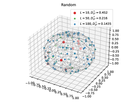
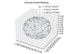
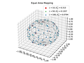
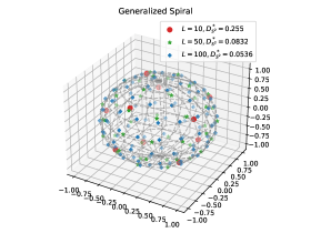
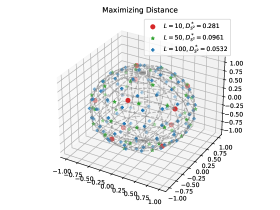
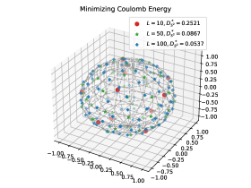
Figure 1: points sets on $\mathbb{S}^{2}$ with the size of $10,50,100$ and the corresponding spherical cap discrepancies.

Spherical cap discrepancy. The most used discrepancy to measure the uniformity of a points set $\theta_{1},\ldots,\theta_{L}\in\mathbb{S}^{d-1}$ is the spherical cap discrepancy [8]:

$$D^{*}_{\mathbb{S}^{d-1}}(\theta_{1},\ldots,\theta_{L})=\sup_{w\in\mathbb{S}^{d-1},t\in[-1,1]}\left|\frac{1}{L}\sum_{l=1}^{L}\textbf{1}_{\theta_{L}\in C(w,t)}-\sigma_{0}(C(w,t))\right|,$$ (7)

where $C(w,t)=\{x\in\mathbb{S}^{d-1}|\langle w,x\rangle\leq t\}$ is a spherical cap, and $\sigma_{0}$ is the law of $\mathcal{U}(\mathbb{S}^{d-1})$. It is proven that $\theta_{1},\ldots,\theta_{L}$ are asymptotically uniformly distributed if $D^{*}_{\mathbb{S}^{d-1}}(\theta_{1},\ldots,\theta_{L})\to 0$ [8]. A points set $\theta_{1},\ldots,\theta_{L}$ is called a low-discrepancy sequence on $\mathbb{S}^{2}$ if $D^{*}_{\mathbb{S}^{2}}(\theta_{1},\ldots,\theta_{L})\in\mathcal{O}(L^{-3/4}\sqrt{\log(L)})$. For some functions in Sobolev spaces, a lower spherical cap discrepancy leads to a better worse-case error [8, 7].

QMC points sets on $\mathbb{S}^{d-1}$. We explore various methods to construct potentially low-discrepancy sequences on the unit hypersphere. Some of these constructions are applicable to any dimension, while others are specifically designed for the 2-dimensional sphere ($\mathbb{S}^{2}$).

Gaussian-based mapping. Utilizing the connection between Gaussian distribution and the uniform distribution over the unit-hypersphere, i.e., $x\sim\mathcal{N}(0,I_{d})$ then $x/\|x\|_{2}\sim\mathcal{U}(\mathbb{S}^{d-1})$, we can map a low discrepancy sequence $x_{1},\ldots,x_{L}$ on $[0,1]^{d}$ to a potential low discrepancy sequence $\theta_{1},\ldots,\theta_{L}$ on $\mathbb{S}^{d-1}$ through the mapping $\theta=f(x)=\Phi^{-1}(x)/\|\Phi^{-1}(x)\|_{2}$ with $\Phi^{-1}$ is the inverse CDF of $\mathcal{N}(0,1)$ (entry-wise). This technique is mentioned in [4] and can be used in any dimension.

Equal area mapping. Following the same idea of transforming a low-discrepancy sequence on the unit grid, we can utilize an equal area mapping (projection) to map from $[0,1]^{2}$ to $\mathbb{S}^{2}$. For instance, we use Lambert cylindrical mapping $f(x,y)=(2\sqrt{y-y^{2}}\cos(2\pi x),2\sqrt{y-y^{2}}\sin(2\pi x),1-2y)$. This approach is proved to create an asymptotic uniform sequence which is empirically shown to be a low-discrepancy sequence on $\mathbb{S}^{2}$ in [2].

Generalized Spiral. We can explicitly construct a $L$-points such that they are equally distributed on $\mathbb{S}^{2}$ with spherical coordinates $(\phi_{1},\phi_{2})$ [48]: $z_{i}=1-\frac{2i-1}{L},\phi_{i1}=\cos^{-1}(z_{i}),\phi_{i2}=1.8\sqrt{L}\phi_{1i}\mod 2\pi$ for $i=1,\ldots,L$. We can map from the spherical coordinates $(\phi_{1},\phi_{2})$ to the conventional coordinates through the mapping $f(\phi_{1},\phi_{2})=(\sin(\phi_{1})\cos(\phi_{2}),\sin(\phi_{1})\sin(\phi_{2}),\cos(\phi_{1}))$. This construction is proven to give an asymptotic uniform sequence in [18] and is empirically shown to have optimal worst-case error in [7] for Sobolev functions.

Maximizing Distance and minimizing Coulomb energy. Previous works [7, 18] suggest that optimizing a points set $\theta_{1},\ldots,\theta_{L}$ such that it maximizing the distance $\sum_{i=1}^{L}\sum_{j=1}^{L}|\theta_{i}-\theta_{j}|$ or minimizing Coulomb energy $\sum_{i=1}^{L}\sum_{j=1}^{L}\frac{1}{|\theta_{i}-\theta_{j}|}$ could create a potentially low-discrepancy sequence. They are shown to achieve optimal worst-case error in [7] though they could suffer from sub-optimal optimization in practice. Minimizing Coulomb energy is proven to create an asymptotic uniform sequence in [15]. In this work, we use generalized spiral points as initialization for these optimization-based points set.

Empirical comparison. We adopt a recent numerical computation of the spherical cap discrepancy [19] to compare the discussed construction of $L$-points sets. We show the visualization and discrepancies for $L=10,50,100$ in Figure 1. Overall, generalized spiral points and optimization-based points yield the lowest discrepancies, followed by the equal area mapping construction. The Gaussian-based mapping construction performs worst among quasi-methods; however, it still yields much lower spherical cap discrepancies than conventional random points. Qualitatively, we observe that the spherical cap discrepancy is consistent with the uniformity of points sets on the unit hypersphere. We also include a comparison with the hypothetical lines of $CL^{-3/4}\sqrt{\log(L)}$ for some constant $C$ in Figure 7 in Appendix D.1. From the results, we observe that the equal area mapping construction, generalized spiral points, and optimization-based construction are low-discrepancy sequences. For convenience, we refer to these sequences as QMC points sets.

3.2 Quasi-Sliced Wasserstein

Quasi-Monte Carlo for SW. Based on the aforementioned QMC points sets in Section 3.1, we can define the QMC approximation of SW distance as follows.

Definition 1.

Given $p\geq 1$, $d\geq 2$, two probability measures $\mu,\nu\in\mathcal{P}_{p}(\mathbb{R}^{d})$, and a Quasi-Monte Carlo points set $\theta_{1},\ldots,\theta_{L}\in\mathbb{S}^{d-1}$, the Quasi-Sliced Wasserstein-$p$ between $\mu$ and $\nu$ is defined as:

$$\widehat{\text{QSW}}^{p}_{p}(\mu,\nu;\theta_{1},\ldots,\theta_{L})=\frac{1}{L}\sum_{l=1}^{L}\text{W}_{p}^{p}(\theta_{l}\sharp\mu,\theta_{l}\sharp\nu).$$ (8)

We refer to Algorithm 2 in Appendix B for the computational algorithm of QSW.

Quasi-Sliced Wasserstein variants. We refer to (i) QSW with Gaussian-based mapping QMC points set as GQSW, (ii) QSW with equal area mapping QMC points set as EQSW, (iii) QSW with QMC generalized spiral points as SQSW, (iv) QSW with maximizing distance QMC points set as DQSW, and (v) QSW with minimizing Coulomb energy sequence as CQSW.

Proposition 1.

With Gaussian-based mapping, equal area mapping, generalized spiral point, and minimizing Coulomb energy, we have $\widehat{\text{QSW}}^{p}_{p}(\mu,\nu;\theta_{1},\ldots,\theta_{L})\to\text{SW}_{p}^{p}(\mu,\nu)$ as $L\to\infty$.

Proof of Proposition 1 is given in Appendix A.1. We now discuss some properties of QSW variants.

Computational complexities. QSW variants are deterministic, which means that the construction of QMC points sets is a one-time cost and can be reused multiple times. Therefore, the computation of QSW variants is the same as SW, i.e., the time complexity is $\mathcal{O}(Ln\log n+Ldn)$, and the space complexity is $\mathcal{O}(Ld+Ln)$. Since QSW does not require resampling the set of projecting directions at each evaluation time, QSW is faster than SW if QMC points sets have been constructed previously.

Gradient Approximation. When dealing with parametric probability measures, e.g., $\nu_{\phi}$, we might be interested in computing the gradient $\nabla_{\phi}\text{SW}p^{p}(\mu,\nu\phi)$ for optimization purposes. When using QMC, we obtain the corresponding deterministic approximation as follows $\nabla_{\phi}\widehat{\text{QSW}}^{p}_{p}(\mu,\nu_{\phi};\theta_{1},\ldots,\theta_{L})=\frac{1}{L}\sum_{l=1}^{L}\nabla_{\phi}\text{W}_{p}^{p}(\theta_{l}\sharp\mu,\theta_{l}\sharp\nu_{\phi})$ for a QMC points set $\theta_{1},\ldots,\theta_{L}$. For a more detailed definition of the gradient of the SW distance, please refer to the work by Tanguy et al. [53]. Since a deterministic gradient approximation may not lead to good convergence in optimization with a sufficiently small $L$, we will develop an unbiased estimation from QMC points sets in the next section.

Related works. Sliced Wasserstein is used as an optimization objective to construct a QMC points set on the unit-cube and the unit-ball in [44]. However, a QMC points set on the unit-hypersphere is not discussed, and sliced Wasserstein here is still approximated by conventional Monte Carlo integration. In contrast to the mentioned work, our focus is on using QMC points sets on the unit-hypersphere to approximate SW. The usage of heuristic scaled mapping with Halton sequence for sliced Wasserstein is briefly mentioned for the comparison between two Gaussians in [33]. In this work, we consider a broader class of QMC points sets, assess their quality with spherical cap discrepancy, discuss their randomized versions, and compare them in real applications. For further discussion on related works, please refer to Appendix C.

3.3 Randomized Quasi-Sliced Wasserstein

While QSW approximations have the potential to improve approximation error, they are all deterministic. Furthermore, the gradient estimator of QSW is a deterministic approximation, which may not be well-suited for optimizing convergence problems with SW as the loss function. Consequently, we introduce Randomized Quasi-Sliced Wasserstein by introducing randomness into QMC points sets.

Randomized Quasi-Monte Carlo. The idea of Randomized Quasi-Monte Carlo (RQMC) is to inject randomness into a given QMC points set. For the unit cube, we can achieve a random QMC points set $x_{1},\ldots,x_{L}$ by shifting [11] i.e., $y_{1}=(x_{i}+U)\text{ mod }1$ for all $i=1,\ldots,L$ and $U\sim\mathcal{U}([0,1]^{d})$. In practice, scrambling [42] is preferable since it gives a uniformly distributed random vector when applying to $x\in[0,1]^{d}$. In greater detail, $x$ is rewritten into $x=\sum_{k=1}^{\infty}b^{-k}a_{k}$ for base $b$ digits and $a_{k}\in\{0,1,\ldots,b-1\}$. After that, we will permute $a_{1},\ldots,a_{k}$ uniform randomly to obtain the scrambled version of $x$. Scrambling is applied for all points in a QMC points set to obtain the randomized QMC points set.

Randomized QMC points sets on $\mathbb{S}^{d-1}$. To the best of our knowledge, there is no prior work of randomized QMC points sets on the unit-hypersphere. Therefore, we discuss two practical ways to obtain random QMC points sets i.e., pushfoward QMC points sets and random rotation.

Pushfoward QMC points sets. Given a randomized QMC points set $x_{1}^{\prime},\ldots,x_{L}^{\prime}$ on the unit-cube (unit-grid), we can use Gaussian-based mapping (or equal area mapping) to create a random QMC points set on the unit-hypersphere $\theta_{1}^{\prime},\ldots,\theta_{L}^{\prime}$. As long as the randomized sequence $x_{1}^{\prime},\ldots,x_{L}^{\prime}$ is low-discrepancy (e.g., using scrambling), the spherical points set $\theta_{1}^{\prime},\ldots,\theta_{L}^{\prime}$ will have the same uniformity as the non-randomized construction.

Random rotation. Given a QMC points set $\theta_{1},\ldots,\theta_{L}$ on the unit-hypersphere $\mathbb{S}^{d-1}$, we can apply uniform random rotation to achieve a random QMC points set. In particular, we first sample $U\sim\mathcal{U}(\mathbb{V}_{d}(\mathbb{R}^{d}))$ where $\mathbb{V}_{d}(\mathbb{R}^{d})=\{U\in\mathbb{R}^{d\times d}|U^{\top}U=I_{d}\}$ is the Stiefel manifold. After that, we form the new sequence $\theta_{1}^{\prime},\ldots,\theta_{L}^{\prime}$ with $\theta_{i}^{\prime}=U\theta_{i}$ for all $i=1,\ldots,L$. Since rotation does not change the norm of vectors, the randomized QMC points set can be still a low-discrepancy sequence of the original QMC points set is low-discrepancy. Moreover, sampling uniformly from the Stiefel manifold is equivalent to applying the Gram-Smith orthogonal process to $z_{1},\ldots,z_{l}\overset{i.i.d}{\sim}\mathcal{N}(0,I_{d})$ (Bartlett decomposition theorem) [35].

Definition 2.

Given $p\geq 1$, $d\geq 2$, two measures $\mu,\nu\in\mathcal{P}_{p}(\mathbb{R}^{d})$, and a randomized Quasi-Monte Carlo points set $\theta_{1}^{\prime},\ldots,\theta_{L}^{\prime}\in\mathbb{S}^{d-1}$, Randomized Quasi-Sliced Wasserstein-$p$ between $\mu$ and $\nu$:

$$\widehat{\text{RQSW}}^{p}_{p}(\mu,\nu;\theta_{1}^{\prime},\ldots,\theta_{L}^{\prime})=\frac{1}{L}\sum_{l=1}^{L}\text{W}_{p}^{p}(\theta_{l}^{\prime}\sharp\mu,\theta_{l}^{\prime}\sharp\nu).$$ (9)

We refer to Algorithm 3-4 for computational algorithms of RQSW.

Randomized Quasi-Sliced Wasserstein variants. For pushfoward QMC points sets, we refer to (i) RQSW with Gaussian-based mapping as RGQSW, (ii) RQSW with equal area mapping as REQSW. For random rotation QMC points sets, we refer to (iii) RQSW with Gaussian-based mapping as RRGQSW, (iv) RQSW with equal area mapping as RREQSW (v) RQSW with generalized spiral points as RSQSW, (vi) RQSW with maximizing distance QMC points set as RDQSW, and (vii) RQSW with minimizing Coulomb energy sequence as RCQSW.

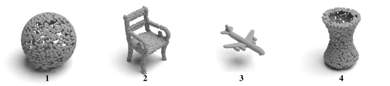
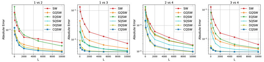
Figure 2: The error for approximation SW distances between empirical distributions over point-clouds.

Proposition 2.

Gaussian-based mapping and random rotation randomized Quasi-Monte Carlo points sets are uniformly distributed, and the corresponding estimators $\text{RQSW}^{p}_{p}(\mu,\nu;\theta_{1}^{\prime},\ldots,\theta_{L}^{\prime})$ are unbiased estimations of $\text{SW}_{p}^{p}(\mu,\nu)$ i.e., $\mathbb{E}[\widehat{\text{RQSW}}^{p}_{p}(\mu,\nu;\theta_{1}^{\prime},\ldots,\theta_{L}^{\prime})]=\text{SW}_{p}^{p}(\mu,\nu)$.

Proof of Proposition 2 is given in Appendix A.2. We now discuss some properties of RQSW variants.

Computational complexities. Compared to QSW, RQSW requires additional computation for randomization. For the push-forward approach, scrambling and shifting cost the time complexity and space complexity of $\mathcal{O}(Ld)$. In addition, mapping the randomized sequence from the unit-cube (unit-grid) to the unit-hypersphere costs $\mathcal{O}(Ld)$ in time complexity. For the random rotation approach, sampling a random rotation matrix costs $\mathcal{O}(d^{3})$. After that, multiplying the sampled rotation matrix with the precomputed QMC points set costs $\mathcal{O}(Ld^{2})$ in time complexity and $\mathcal{O}(Ld)$ in space complexity. Overall, in the 3D setting where $d=3$ and $n>>L>d$, the addition computation for RQSW is negligible compared to the order of $n\log n$ from computing one-dimensional Wasserstein.

Gradient estimation. In contrast to QSW, RQSW is a random estimation. In addition, it is an unbiased estimation with the proposed construction of randomized QSW points sets from Proposition 2. Therefore, it follows directly that $\mathbb{E}[\nabla_{\phi}\widehat{\text{RQSW}}^{p}_{p}(\mu,\nu_{\phi};\theta_{1}^{\prime},\ldots,\theta_{L}^{\prime})]=\nabla_{\phi}\text{SW}_{p}^{p}(\mu,\nu_{\phi})$ due to the Leibniz rule. Therefore, this estimation of gradient can lead to better convergence for optimization.

Table 1: Summary of Wasserstein-2 distances (multiplied by $10^{2}$) from three different runs.

Estimators	Step 100 ($\text{W}_{2}\downarrow$)	Step 200 ($\text{W}_{2}\downarrow$)	Step 300 ($\text{W}_{2}\downarrow$)	Step 400($\text{W}_{2}\downarrow$)	Step 500 ($\text{W}_{2}\downarrow$)
SW	$5.761\pm 0.088$	$0.178\pm 0.001$	$0.025\pm 0.001$	$0.01\pm 0.001$	$0.004\pm 0.001$
GQSW	$6.136\pm 0.0$	$0.255\pm 0.0$	$0.077\pm 0.0$	$0.07\pm 0.0$	$0.068\pm 0.0$
EQSW	$\mathbf{5.414\pm 0.0}$	$0.22\pm 0.0$	$0.079\pm 0.0$	$0.071\pm 0.0$	$0.069\pm 0.0$
SQSW	$5.718\pm 0.0$	$0.181\pm 0.0$	$0.075\pm 0.0$	$0.07\pm 0.0$	$0.069\pm 0.0$
DQSW	$5.792\pm 0.0$	$0.193\pm 0.0$	$0.077\pm 0.0$	$0.07\pm 0.0$	$0.067\pm 0.0$
CQSW	$5.609\pm 0.0$	$\mathbf{0.163\pm 0.0}$	$0.07\pm 0.0$	$0.066\pm 0.0$	$0.065\pm 0.0$
RGQSW	$5.727\pm 0.035$	$0.169\pm 0.003$	$0.022\pm 0.001$	$0.007\pm 0.001$	$0.003\pm 0.001$
RRGQSW	$5.733\pm 0.027$	$0.168\pm 0.006$	$0.025\pm 0.003$	$0.011\pm 0.002$	$0.006\pm 0.001$
REQSW	$5.737\pm 0.017$	$0.171\pm 0.004$	$0.022\pm 0.002$	$0.007\pm 0.001$	$0.003\pm 0.001$
RREQSW	$5.704\pm 0.011$	$0.165\pm 0.004$	$0.021\pm 0.0$	$0.007\pm 0.001$	$0.003\pm 0.001$
RSQSW	$5.722\pm 0.0$	$0.169\pm 0.001$	$0.021\pm 0.001$	$0.007\pm 0.001$	$\mathbf{0.002\pm 0.0}$
RDQSW	$5.725\pm 0.002$	$0.169\pm 0.001$	$0.023\pm 0.002$	$0.009\pm 0.002$	$0.003\pm 0.002$
RCQSW	$5.721\pm 0.002$	$0.167\pm 0.002$	$\mathbf{0.02\pm 0.0}$	$\mathbf{0.007\pm 0.001}$	$0.003\pm 0.001$

4 Experiments

In this section, we first demonstrate that QSW variants outperform the conventional Monte Carlo approximation (referred to as SW) in Section 4.1. We then showcase the advantages of RQSW variants in point-cloud interpolation and image style transfer, comparing them to both QSW variants and the conventional SW approximation in Section 4.2 and Section 4.3, respectively. Finally, we present the favorable performance of QSW and RQSW variants in training a deep point-cloud autoencoder

4.1 Approximation Error

Settings. We select randomly four point-clouds (1, 2, 3, and 4 with 3 dimensions, $2048$ points) from ShapeNet Core-55 dataset [9] as shown in Figure 2. After that, we use MC estimation with $L=100000$ to approximate $SW_{2}^{2}$ between empirical distributions over point-clouds 1-2, 1-3, 2-3, and 3-4, then treat them as the population value. Next, we vary $L$ in the set $\{10,100,500,1000,2000,5000,10000\}$ and compute the corresponding absolute error of the estimation from MC (SW), and QMC (QSWs).

Results. We illustrate the approximation errors in Figure 1. From the figure, it is evident that QSW approximations yield lower errors compared to the conventional SW approximation. Among the QSW approximations, CQSW and DQSW perform the best, followed by SQSW. In this simulation, the quality of GQSW and EQSW is not comparable to the previously mentioned approximations. Nevertheless, their errors are at least comparable to SW and are considerably better most of the time.

4.2 Point-cloud interpolation

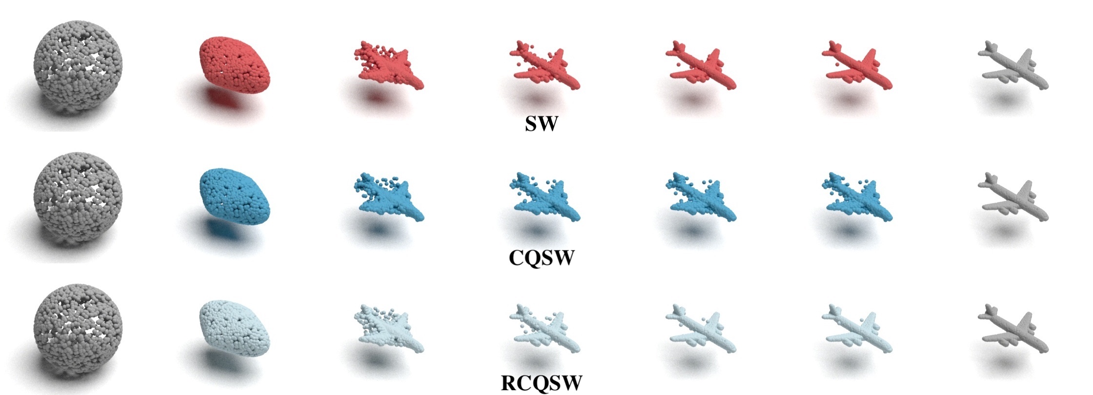
Figure 3: Point-cloud interpolation from SW, CQSW, and RCQSW with $L=100$.

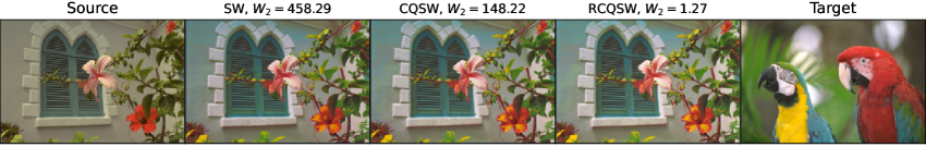
Figure 4: Style-transferred images from SW, CQSW, and RCQSW with $L=100$.

Settings. To interpolate between two point-clouds $X$ and $Y$, we define the curve $\dot{Z}(t)=-n\nabla_{Z(t)}\left[\text{SW}_{2}\left(P_{Z(t)},P_{Y}\right)\right]$ where $P_{X}$ and $P_{Y}$ are empirical distributions over $X$ and $Y$ in turn. Here, the curve starts from $Z(0)=X$ and ends at $Y$. In this experiment, we set $X$ as the point-cloud 1 and Y as the point-cloud 3 in Figure 2. After that, we use different gradient approximations from the conventional SW, QSW variants, and RQSW variants to perform the Euler scheme with 500 iterations, step size $0.01$. To verify which approximation gives the shortest curve in length, we compute Wasserstein-2 distance (POT library [14]) between $P_{Z(t)}$ and $P_{Y}$.

Results. We report Wasserstein-2 distances (from three different runs) between $P_{Z(t)}$ and $P_{Y}$ at time step $100,200,300,400,500$ in Table 1 with $L=100$. From the table, we observe that QSW variants do not perform well in this application due to the deterministic approximation of the gradient with a fixed set of projecting directions. In particular, although EQSW and CQSW perform the best at time steps 100 and 200, QSW variants cannot make the curves terminate. As expected, RQSW variants can solve the issue by injecting randomness to create new random projecting directions. Compared to SW, RQSW variants are all better except RRGQSW. We visualize the interpolation for SW, CQSW, and RCQSW in Figure 3. The full visualization from all approximations is given in Figure 8 in Appendix D.2. From the figures, we observe that the qualitative comparison is consistent with the quantitative comparison in Table 1. In Appendix D.2, we also provide the result for $L=10$ in Table 3, and the result for a different pair of point-clouds in Table 4-5 and Figure 9. We refer the reader to Appendix D.2 for a more detailed discussion.

4.3 Image Style Transfer

Settings. Given a source image and a target image, we denote the associated color palette as $X$ and $Y$ which are matrices of size $n\times 3$ ($n$ is the number of pixels). Similar to point-cloud interpolation, we iterate along the curve between $P_{X}$ and $P_{Y}$. However, since the value of the color palette (RGB) is in set $\{0,\ldots,255\}$, we need to do an additional rounding step at the final Euler iterations. Moreover, we use more iterations i.e., $1000$, and a bigger step size i.e., $1$.

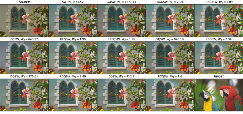
Figure 11: Style-transferred images from SW, QSW variants, and RQSW variants with $L=100$.

Results. For $L=100$, we report Wasserstein-2 distances at the final time step and the corresponding transferred images from SW, CQSW, and RCQSW in Figure 4. The full results for all approximations are given in Figure 10 in Appendix D.3. In addition, we provide results for $L=10$ in Figure 11 in Appendix D.3. Overall, QSW variants and RQSW perform better than SW in terms of both Wasserstein distance and visualization (brighter transferred images). Compared between QSW and RQSW, RQSW gives considerably lower Wasserstein distances. In this task, RQSW variants yield quite similar performance. We refer the reader to Appendix D.3 for a more detailed discussion.

4.4 Deep Point-cloud Autoencoder

Settings. We follow the experimental setting in [40] to train deep point-cloud autoencoders with SW distance on the ShapeNet Core-55 dataset [9]. We aim to optimize the following objective $\min_{\phi,\gamma}\mathbb{E}_{X\sim\mu(X)}[\text{SW}_{p}(P_{X},P_{g_{\gamma}(f_{\phi}(X)))}],$ where $\mu(X)$ is our data distribution, $f_{\phi}$ and $g_{\psi}$ are a deep encoder and a deep decoder with Point-Net [47] architecture. To optimize the objective, we use the conventional MC estimation, QSW, and RQSW to approximate the gradient $\nabla_{\phi}$ and $\nabla_{\psi}$. We then utilize the standard SGD optimizer to train the autoencoder (with an embedding size of 256) for 400 epochs with a learning rate of 1e-3, a batch size of 128, a momentum of 0.9, and a weight decay of 5e-4. To evaluate the quality of trained autoencoders, we compute the average reconstruction losses, which are $\text{W}_{2}$ distance and $\text{SW}_{2}$ distance (estimated with 10000 MC samples), on a different dataset i.e., ModelNet40 dataset [55].

Results. We report the reconstruction losses with $L=100$ in Table 2 (from three different training times). Interestingly, CQSW performs the best among all approximations i.e., SW, QSW variants, and RQSW variants at the last epoch. We have an explanation for this phenomenon. In contrast to point-cloud interpolation which considers only one pair of point-clouds, we estimate an autoencoder from an entire dataset of point-clouds. Therefore, model misspecification might happen here i.e., the family of the Point-Net autoencoder does not contain the true data-generating distribution. Hence, $L=100$ might be large enough to approximate well with QSW. When we reduce $L$ to $10$ in Table 6 in Appendix 4.4, CQSW and other QSW variants become considerably worse. In this application, we also observe that GQSW suffers from some numerical issues which leads to a very poor performance. As a solution for the mentioned problems, RQSW performs consistently well compared to SW especially random rotation variants. We present some reconstructed point-clouds from SW, CQSW, and RCQSW in Figure 5 and full visualization in Figure 12- 13. Overall, we recommend RCQSW for this task as a safe choice. We refer the reader to Appendix D.4 for a more detailed discussion.

Table 2: Reconstruction losses (multiplied by 100) from trained by different approximations with $L=100$.

Approximation	Epoch 100		Epoch 200		Epoch 400
	$\text{SW}_{2}$($\downarrow$)	$\text{W}_{2}$($\downarrow$)	$\text{SW}_{2}$ ($\downarrow$)	$\text{W}_{2}$($\downarrow$)	$\text{SW}_{2}$ ($\downarrow$)	$\text{W}_{2}$($\downarrow$)
SW	$2.25\pm 0.06$	$10.58\pm 0.12$	$2.11\pm 0.04$	$9.92\pm 0.08$	$1.94\pm 0.06$	$9.21\pm 0.06$
GQSW	$11.17\pm 0.07$	$32.58\pm 0.06$	$11.75\pm 0.07$	$33.27\pm 0.09$	$14.82\pm 0.02$	$37.99\pm 0.05$
EQSW	$2.25\pm 0.02$	$10.57\pm 0.02$	$2.05\pm 0.02$	$9.84\pm 0.07$	$1.90\pm 0.04$	$9.20\pm 0.07$
SQSW	$2.25\pm 0.01$	$10.57\pm 0.03$	$2.08\pm 0.01$	$9.90\pm 0.04$	$1.90\pm 0.02$	$9.17\pm 0.05$
DQSW	$2.24\pm 0.07$	$10.58\pm 0.05$	$2.06\pm 0.04$	$9.83\pm 0.01$	$1.86\pm 0.05$	$9.12\pm 0.07$
CQSW	$2.22\pm 0.02$	$10.54\pm 0.02$	$2.05\pm 0.06$	$\mathbf{9.81\pm 0.04}$	$\mathbf{1.84\pm 0.02}$	$\mathbf{9.06\pm 0.02}$
RGQSW	$2.25\pm 0.02$	$10.57\pm 0.01$	$2.09\pm 0.03$	$9.92\pm 0.01$	$1.94\pm 0.02$	$9.18\pm 0.02$
RRGQSW	$2.23\pm 0.01$	$10.51\pm 0.04$	$2.06\pm 0.05$	$9.84\pm 0.06$	$1.88\pm 0.09$	$9.16\pm 0.11$
REQSW	$2.24\pm 0.04$	$10.53\pm 0.04$	$2.08\pm 0.04$	$9.90\pm 0.08$	$1.89\pm 0.04$	$9.17\pm 0.06$
RREQSW	$2.21\pm 0.04$	$10.50\pm 0.04$	$2.03\pm 0.02$	$9.83\pm 0.02$	$1.88\pm 0.05$	$9.15\pm 0.06$
RSQSW	$2.22\pm 0.05$	$10.53\pm 0.01$	$2.04\pm 0.06$	$9.82\pm 0.06$	$1.85\pm 0.05$	$9.12\pm 0.02$
RDQSW	$\mathbf{2.21\pm 0.03}$	$\mathbf{10.50\pm 0.02}$	$2.03\pm 0.04$	$9.82\pm 0.04$	$1.86\pm 0.03$	$9.12\pm 0.02$
RCQSW	$2.22\pm 0.03$	$10.50\pm 0.05$	$\mathbf{2.03\pm 0.02}$	$9.82\pm 0.03$	$1.85\pm 0.06$	$9.12\pm 0.03$

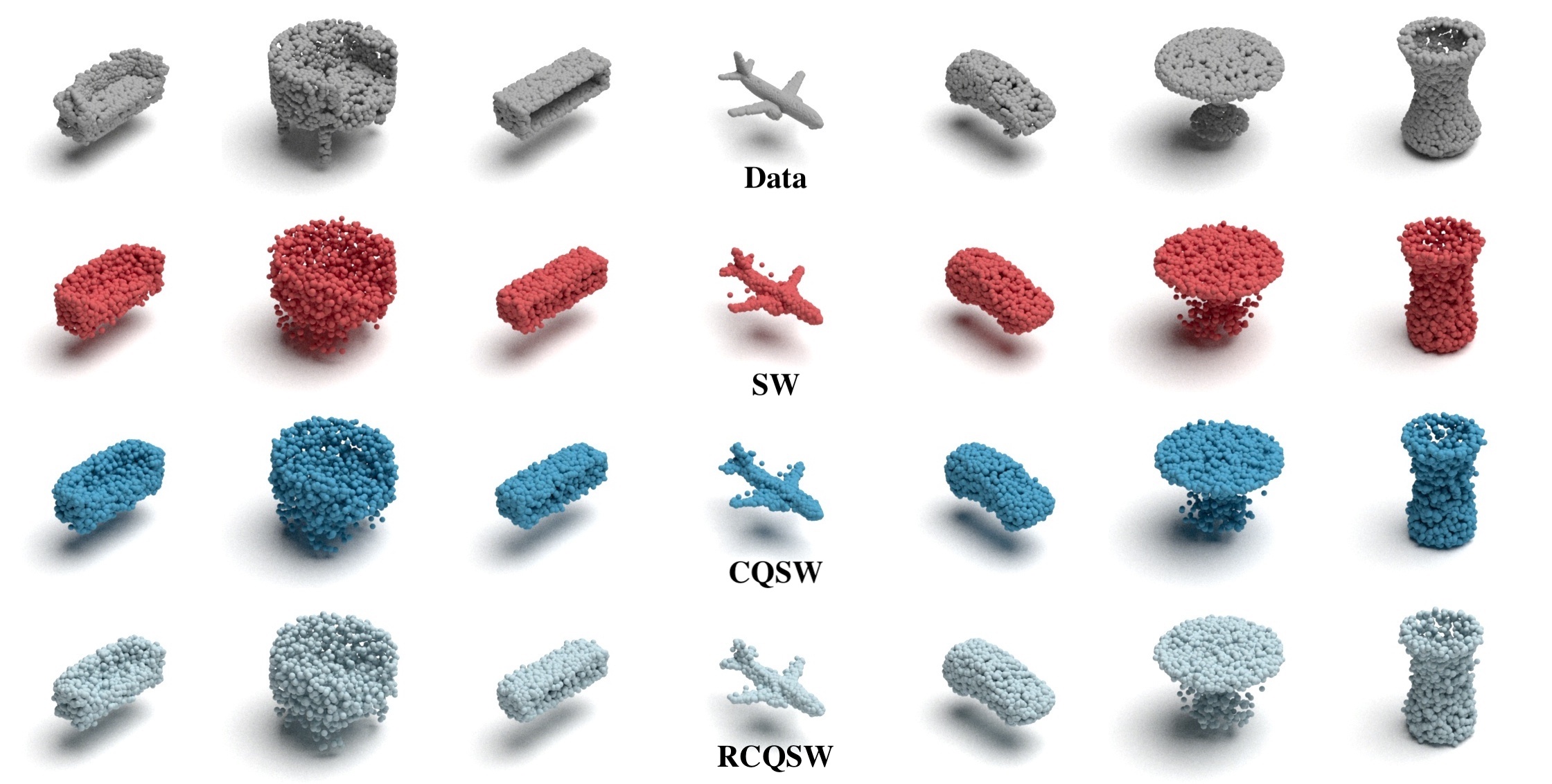
Figure 5: Reconstructed point-clouds from SW, cQSW, and RCQSW with $L=100$.

5 Conclusion

We presented Quasi-Sliced Wasserstein (QSW) which is a better class of numerical approximations for sliced Wasserstein (SW) distance based on Quasi-Monte Carlo (QMC). We discussed various ways to construct QMC points sets on the unit hypersphere including Gaussian-based mapping, equal area mapping, generalized spiral points, maximizing distance, and minimizing Coulomb energy. Moreover, we proposed Randomized Quasi-Sliced Wasserstein (RQSW) which is a family of unbiased estimators of SW distance which is based on randomizing constructed QMC points sets. We showed that QSW can reduce approximation error on comparing 3D point clouds. In addition, we showed that QSW variants and RQSW variants provide better gradient approximation for point-cloud interpolation, image-style transfer, and training point-cloud autoencoder. Overall, we recommend RQSW with random rotation of minimizing Coulomb energy QMC points set since it gives consistent and stable behavior across tested applications. In the future, we will extend QSW and RQSW to a higher dimension i.e., $d>3$, and apply QMC to other variants of SW distance.

Appendix A Proofs

A.1 Proof of Proposition 1

We first discuss the asymptotic uniformity of the mentioned QMC points set.

For the Gaussian-based mapping construction, From the construction, we have the function $\theta=f(x)=\frac{\Phi^{-1}(x)}{||\Phi^{-1}(x)||_{2}}$. Given a Sobol sequence $x_{1},\ldots,x_{L}$, the corresponding spherical vectors $\theta_{1},\ldots,\theta_{L}$ with $\theta_{l}=f(x_{L})$ for all $l=1,\ldots,L$. Let $X_{L}\sim\frac{1}{L}\sum_{l=1}^{L}\delta_{x_{l}}$, from the low discrepancy sequence property of Sobol sequences [52], we have $X_{L}$ converges to $X\sim\mathcal{U}(0,1)$ in distribution as $L\to\infty$. Since our function $f(x)$ is continuous on $[0,1]^{d}$, using continuous mapping theorem, we have $f(X_{L})$ converges to $f(X)$ in distribution as $L\to\infty$, which means that $\frac{1}{L}\sum_{l=1}^{L}\delta_{\theta_{i}}$ converge to the pdf of $\mathcal{U}(\mathbb{S}^{d-1})$ as $L\to\infty$ since $f(X)\sim\mathcal{U}(\mathbb{S}^{d-1})$. For the equal area mapping construction, we refer the reader to the work [2] for the proof of uniformity. For the generalized spiral points construction, we refer the reader to the work [18] for the proof of uniformity of this construction. Minimizing Coulomb energy is proven to create an asymptotic uniform sequence in [15].

We denote $\gamma_{L}\sim\frac{1}{L}\sum_{i=1}^{L}\delta_{\theta_{i}l}$ and $\theta\sim\mathcal{U}(\mathbb{S}^{d-1})$. Given an asymptotic uniform points sets $\theta_{1},\ldots,\theta_{L}$, we have $\gamma_{L}\overset{d}{\to}\theta$. Moreover, we have:

$$\text{W}_{p}^{p}(\gamma_{L}\sharp\mu,\gamma_{L}\sharp\nu) =\inf_{\pi\in\Pi(\mu,\nu)}\mathbb{E}_{(x,y)\sim\pi(x,y)}[|\gamma_{L}^{\top}x-\gamma_{L}^{\top}y|_{p}^{p}]$$

$$\leq\inf_{\pi\in\Pi(\mu,\nu)}\mathbb{E}_{(x,y)\sim\pi(x,y)}[\|\gamma_{L}|\|^{p}\|x-y\|^{p}]$$

$$=\inf_{\pi\in\Pi(\mu,\nu)}\mathbb{E}_{(x,y)\sim\pi(x,y)}[\|x-y\|^{p}]$$

$$=\text{W}^{p}_{p}(\mu,\nu),$$

where the first inequality is due to the Cauchy–Schwarz inequality, and the second equality is due to the fact that $\gamma_{L}\in\mathcal{P}(\mathbb{S}^{d-1})$. Since the Wasserstein distance is bounded i.e.,$\text{W}_{p}(\mu,\nu)\leq\infty$, using Dominated Convergence Theorem, we have $\mathbb{E}_{\theta\sim\gamma_{L}}[\text{W}_{p}^{p}(\gamma_{L}\sharp\mu,\gamma_{L}\sharp\nu)]\to\mathbb{E}_{\theta\sim\mathcal{U}(\mathbb{S}^{d-1})}[\text{W}_{p}^{p}(\theta\sharp\mu,\theta\sharp\nu)]$, namely, $\text{QSW}^{p}_{p}(\mu,\nu;\theta_{1},\ldots,\theta_{L})\to\text{SW}_{p}^{p}(\mu,\nu)$ which completes the proof.

A.2 Proof of Proposition 2

For the Gaussian-based mapping construction. given a Sobol sequence $x_{1},\ldots,x_{L}\in[0,1]^{d}$, applying scrambling returns $x_{1}^{\prime},\ldots,x_{L}^{\prime}\in\mathcal{U}([0,1]^{d})$ [42]. Since $f(x)=\frac{\Phi^{-1}(x)}{||\Phi^{-1}(x)||_{2}}$ is the normalized inverse Gaussian CDF, $\theta_{l}^{\prime}=f(x_{l}^{\prime})\sim\mathcal{U}(\mathbb{S}^{d-1})$ for all $l=1,\ldots,L$.

For the random rotation construction, given a fixed vector $\theta\in\mathbb{S}^{d-1}$ and $U=(u_{1},\ldots,u_{d})\sim\mathcal{U}(\mathbb{V}_{d}(\mathbb{R}^{d})$, we now prove that $U\theta\sim\mathcal{U}(\mathbb{S}^{d-1})$. For any $U_{1}\in\mathbb{V}_{d}(\mathbb{R}^{d})$, we have $U_{1}U=U_{2}$ with $U_{2}\sim\mathcal{U}(\mathbb{V}_{d}(\mathbb{R}^{d})$. Therefore, we have $U\theta$ have the same distribution as $U_{1}U\theta$. Since there is only one distribution on $\mathbb{S}^{d-1}$ is invariant to rotation (Theorem 3.7 in [34]) which is the uniform distribution, $U\theta\sim\mathcal{U}(\mathbb{S}^{d-1})$. Therefore, we have the set $\theta_{1}^{\prime},\ldots,\theta_{L}^{\prime}$, which are created by uniformly random rotating a points set $\theta_{1},\ldots,\theta_{L}$, are uniformly distributed.

Now, given $\theta_{1}^{\prime},\ldots,\theta_{L}^{\prime}\sim\mathcal{U}(\mathbb{S}^{d-1})$, we have

$$\mathbb{E}[\widehat{\text{RQSW}}^{p}_{p}(\mu,\nu;\theta_{1}^{\prime},\ldots,\theta_{L}^{\prime})] =\mathbb{E}\left[\frac{1}{L}\sum_{l=1}^{L}\text{W}_{p}^{p}(\theta_{l}^{\prime}\sharp\mu,\theta_{l}^{\prime}\sharp\nu)\right]$$

$$=\frac{1}{L}\sum_{l=1}^{L}\mathbb{E}[\text{W}_{p}^{p}(\theta_{l}^{\prime}\sharp\mu,\theta_{l}^{\prime}\sharp\nu)]$$

$$=\frac{1}{L}\sum_{l=1}^{L}\text{SW}_{p}^{p}(\mu,\nu)=\text{SW}_{p}^{p}(\mu,\nu),$$

which completes the proof.

Appendix B Additional Background

Wasserstein distance. Given two probability measures $\mu\in\mathcal{P}_{p}(\mathbb{R}^{d})$ and $\nu\in\mathcal{P}_{p}(\mathbb{R}^{d})$, and $p\geq 1$, the Wasserstein distance [54, 45] between $\mu$ and $\nu$ is :

$$\text{W}_{p}^{p}(\mu,\nu)=\inf_{\pi\in\Pi(\mu,\nu)}\int_{\mathbb{R}^{d}\times\mathbb{R}^{d}}\|x-y\|_{p}^{p}d\pi(x,y),$$ (10)

where $\Pi(\mu,\nu)$ is set of all couplings that have marginals are $\mu$ and $\nu$ respectively. Considering the discrete case, namely, $\mu=\sum_{i=1}^{n}\alpha_{i}\delta_{x_{i}}$ and $\nu=\sum_{j=1}^{n}\beta_{j}\delta_{y_{j}}$ with $\sum_{i=1}^{n}\alpha_{i}=\sum_{j=1}^{n}\beta_{j}$. The Wasserstein distance between $\mu$ and $\nu$ can be rewritten as:

$$\text{W}_{p}^{p}(\mu,\nu)=\min_{\pi\in\Pi(\mathbf{\alpha},\mathbf{\beta})}\sum_{i=1}^{n}\sum_{j=1}^{n}\pi_{ij}||x_{i}-y_{j}||_{p}^{p},$$ (11)

where $\Pi(\mu,\nu)=\{\pi\in\mathbb{R}^{n\times n}_{+}|\pi\mathbf{1}=\mathbf{\alpha},\pi^{\top}\mathbf{1}=\mathbf{\beta}\}$. Using linear programming, the computational complexity and memory complexity of Wasserstein distance are $\mathcal{O}(n^{3}\log n)$ and $\mathcal{O}(n^{2})$.

Algorithms. We first introduce the computational algorithm for Monte Carlo estimation of SW in Algorithm 1. Next, we provide the algorithm for QMC approximation of SW in Algorithm 2. Finally, we present the algorithms for Randomized QMC estimation of SW with scrambling and random rotation in Algorithms 3 and  4, respectively.

Algorithm 1 The Monte Carlo estimation of sliced Wasserstein distance.

  Input: Probability measures $\mu$ and $\nu$, $p>1$, and the number of projections $L$.

  Set $\widehat{\text{SW}}_{p}^{p}(\mu,\nu;L)=0$

  for $l=1$ to $L$ do

     Sample $\theta_{l}\sim\mathcal{U}(\mathbb{S}^{d-1})$

     Compute $\widehat{\text{SW}}_{p}^{p}(\mu,\nu;L)=\widehat{\text{SW}}_{p}^{p}(\mu,\nu;L)+\frac{1}{L}\int_{0}^{1}|F_{\theta_{l}\sharp\mu}^{-1}(z)-F_{\theta_{l}\sharp\nu}^{-1}(z)|^{p}dz$

  end for

  Return: $\widehat{\text{SW}}_{p}^{p}(\mu,\nu;L)$

Algorithm 2 The Quasi-Monte Carlo approximation of sliced Wasserstein distance.

  Input: Probability measures $\mu$ and $\nu$, $p>1$, QMC points set $\theta_{1},\ldots,\theta_{L}\in\mathbb{S}^{d-1}$.

  Set $\widehat{\text{QSW}}_{p}^{p}(\mu,\nu;\theta_{1},\ldots,\theta_{L})=0$

  for $l=1$ to $L$ do

     Compute $\widehat{\text{QSW}}_{p}^{p}(\mu,\nu;\theta_{1},\ldots,\theta_{L})=\widehat{\text{QSW}}_{p}^{p}(\mu,\nu;\theta_{1},\ldots,\theta_{L})+\frac{1}{L}\int_{0}^{1}|F_{\theta_{l}\sharp\mu}^{-1}(z)-F_{\theta_{l}\sharp\nu}^{-1}(z)|^{p}dz$

  end for

  Return: $\widehat{\text{QSW}}_{p}^{p}(\mu,\nu;\theta_{1},\ldots,\theta_{L})$

Algorithm 3 The Randomized Quasi-Monte Carlo estimation of sliced Wasserstein distance with scrambling.

  Input: Probability measures $\mu$ and $\nu$, $p>1$, QMC points set $x_{1},\ldots,x_{L}\in[0,1]^{d}$.

  Scrambling $x_{1},\ldots,x_{L}$ to obtain $x_{1}^{\prime},\ldots,x_{L}^{\prime}$

  Compute $\theta_{1}^{\prime},\ldots,\theta_{L}^{\prime}=f(x_{1}^{\prime}),\ldots,f(x_{L}^{\prime})$ for $f$ is the Gaussian-based mapping or the equal area mapping.

  Set $\widehat{\text{RQSW}}_{p}^{p}(\mu,\nu;\theta_{1}^{\prime},\ldots,\theta_{L}^{\prime})=0$

  Randomized

  for $l=1$ to $L$ do

     Compute $\widehat{\text{RQSW}}_{p}^{p}(\mu,\nu;\theta_{1}^{\prime},\ldots,\theta_{L}^{\prime})=\widehat{\text{RQSW}}_{p}^{p}(\mu,\nu;\theta_{1}^{\prime},\ldots,\theta_{L}^{\prime})+\frac{1}{L}\int_{0}^{1}|F_{\theta_{l}^{\prime}\sharp\mu}^{-1}(z)-F_{\theta_{l}^{\prime}\sharp\nu}^{-1}(z)|^{p}dz$

  end for

  Return: $\widehat{\text{RQSW}}_{p}^{p}(\mu,\nu;\theta_{1}^{\prime},\ldots,\theta_{L}^{\prime})$

Algorithm 4 The Randomized Quasi-Monte Carlo estimation of sliced Wasserstein distance with random rotation.

  Input: Probability measures $\mu$ and $\nu$, $p\geq 1$, QMC points set $\theta_{1},\ldots,\theta_{L}\in\mathbb{S}^{d-1}$.

  Sample $U\sim\mathcal{U}(\mathbb{V}_{d}(\mathbb{R}^{d}))$

  Compute $\theta_{1}^{\prime},\ldots,\theta_{L}^{\prime}=U\theta_{1},\ldots,U\theta_{L}$

  Set $\widehat{\text{RQSW}}_{p}^{p}(\mu,\nu;\theta_{1}^{\prime},\ldots,\theta_{L}^{\prime})=0$

  Randomized

  for $l=1$ to $L$ do

     Compute $\widehat{\text{RQSW}}_{p}^{p}(\mu,\nu;\theta_{1}^{\prime},\ldots,\theta_{L}^{\prime})=\widehat{\text{RQSW}}_{p}^{p}(\mu,\nu;\theta_{1}^{\prime},\ldots,\theta_{L}^{\prime})+\frac{1}{L}\int_{0}^{1}|F_{\theta_{l}^{\prime}\sharp\mu}^{-1}(z)-F_{\theta_{l}^{\prime}\sharp\nu}^{-1}(z)|^{p}dz$

  end for

  Return: $\widehat{\text{RQSW}}_{p}^{p}(\mu,\nu;\theta_{1}^{\prime},\ldots,\theta_{L}^{\prime})$

Generation of Sobol sequence. From [24], for generating a Sobol points set $x_{1},\ldots,x_{L}\in[0,1]^{d}$, we need to follow the following procedure. For $j$-th of the points, we need to choose a primitive polynomial of some degree $s_{l}$ in the field $\mathbb{Z}_{2}$ (set of integer of module 2), that is:

$$z^{s_{j}}+a_{1,j}z^{s_{j}-1}+\ldots+a_{s_{j}-1,j}z+1,$$

where the coefficients $a_{1,j},\ldots,a_{s_{j}-1,j}$ are either 0 or 1. We then use $a_{1,j},\ldots,a_{s_{j}-1,j}$ to define a sequence $m_{1,j},m_{2,j},\ldots m_{s_{j},j}$ such that:

$$m_{k,j}=2a_{1,j}m_{k-1,j}\oplus 2^{2}a_{2,j}m_{k-2,j}\oplus\ldots\oplus 2^{s_{j}-1}a_{s_{j}-1,j}m_{k-s_{j}+1,j}\oplus 2^{s_{j}}m_{k-s_{j},1}\oplus m_{k-s_{j},j},$$

for $k>s_{j}+1$ and $\oplus$ is the bit-by-bit exclusive-OR operator. The initial values of $m_{1,j},m_{2,j},\ldots m_{s_{j},j}$ are chosen freely such that $m_{k,j}$, $1\leq k\leq s_{j}$ is odd and less than $2^{k}$. After that, direction numbers $v_{1,j},v_{2,j},\ldots v_{s_{j},j}$ are defined as:

$$v_{k,j}=\frac{m_{k,j}}{2^{k}}.$$

Finally, we have:

$$x_{l,j}=b_{1}v_{1,j}\oplus b_{2}v_{2,j}\oplus\ldots,\oplus b_{s_{j}}v_{s_{j},j},$$

where $b_{i}$ is the $i$-th bit from the right when $l$ is written in binary ,i.e, , $(\ldots b_{2}b_{1})^{2}$ is the binary representation of $l$. For greater detail, we refer the reader to [24] for more detailed and practical algorithms.

Appendix C Related works

Beyond the uniform slicing distribution. Recent works have explored non-uniform slicing distributions [39, 38]. Nevertheless, the uniform distribution remains foundational in constructing the pushforward slicing distribution [39] and the proposal distribution [38]. Consequently, Quasi-Monte Carlo methods can also enhance the approximation of the uniform distribution.

Beyond 3D. It is worth noting that the Gaussian-based construction, maximizing distance, and minimizing Coulomb energy can be applied directly in higher dimensions, i.e., $d>3$. Similarly, their randomized versions could also be used directly in higher dimensions. However, the quality of QMC points sets in high dimensions and their approximation errors are still open questions and require a detailed investigation. Therefore, we will leave this exploration to future work

Scaled Mapping. Quasi-Monte Carlo is briefly used for SW in [33]. In particular, the authors utilize the Halton sequence in the three-dimensional unit cube, then map them to the unit sphere via the scaled mapping $f(x)=\frac{x}{|x|_{2}}$. However, this construction is heuristic and lacks meaningful properties. We visualize points sets of sizes $10,50,100$ in Figure 6. From the figure, it is evident that this construction does not exhibit low-discrepancy behavior, as all points are concentrated in one region of the sphere.

Near Orthogonal Monte Carlo. Motivated by orthogonal Monte Carlo, the authors in [33] propose near-orthogonal Monte Carlo, aiming to make the angles between any two samples close to orthogonal. We utilized the published code for optimization-based approaches available at https://github.com/HL-hanlin/OMC to generate points sets of size $L$ in three dimensions, where $L$ is chosen from the set ${10,50,100}$. For our experiments, we generated only one batch of $L$ points, avoiding the need to specify the second hyperparameter related to the number of batches. We visualize the resulting points sets and their corresponding spherical cap discrepancies in Figure 6. From the figure, it is evident that NOMC yields better spherical cap discrepancies compared to conventional Monte Carlo methods. However, it is important to note that NOMC does not achieve the same level of performance as the QMC points sets we discuss in this work. In this study, our primary focus is on QMC methods, and as such, we leave a detailed investigation of the application of OMC methods for SW to future research.

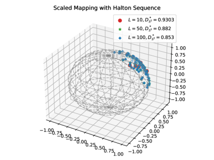
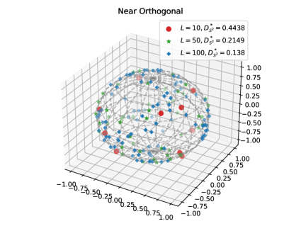
Figure 6: Optimization-based Orthogonal Monte Carlo points set and scaled mapping with Halton Sequence points set.

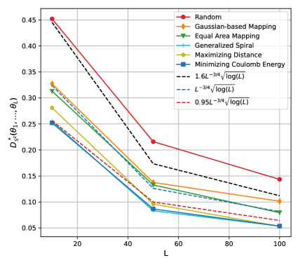
Figure 7: Spherical cap discrepancies of different QMC points sets and random points set.

Appendix D Detailed Experiments

D.1 Spherical Cap Discrepancy

We plotted the spherical cap discrepancies of the discussed QMC point sets and added hypothetical lines of $CL^{-3/4}\sqrt{\log(L)}$ for $C=1.6,C=1,C=0.95$ in Figure 7. From the figure, it is evident that QMC point sets derived from generalized spiral points, maximizing distance, and minimizing Coulomb energy exhibit a faster convergence rate than $\mathcal{O}(L^{-3/4}\sqrt{\log(L)})$. Consequently, they can be classified as low-discrepancy sequences. Regarding the equal-area mapping construction, it demonstrates approximately the same convergence rate as $\mathcal{O}(L^{-3/4}\sqrt{\log(L)})$, suggesting its potential as a low-discrepancy sequence. However, Gaussian-based mapping QMC point sets and random (MC) point sets do not exhibit low-discrepancy behavior. In summary, we recommend using generalized spiral points, maximizing distance, and minimizing Coulomb energy point sets for approximating SW when distance values are a critical factor in the application.

D.2 Point-cloud Interpolation

Approximate Euler methods. We want to iterate through the curve $\dot{Z}(t)=-n\nabla_{Z(t)}\left[\text{SW}2\left(P{Z(t)},P_{Y}\right)\right]$. For each iteration with $t=1,\ldots,T$, we first construct a point set $\theta_{1},\ldots,\theta_{L}$ based on the discussed approaches using MC, QMC methods, and randomized QMC methods. After that, with a step size $\eta>0$, we update:

$$Z(t)=Z(t-1)-n\eta\nabla_{Z(t-1)}\left[\frac{1}{L}\sum_{l=1}^{L}\text{W}_{2}^{2}\left(\theta_{l}\sharp P_{Z(t-1)},\theta_{l}\sharp P_{Y}\right)\right]^{1/2}.$$

Visualization for $L=100$. In addition to the partial visualization in the main text, we provide a full visualization of point-cloud interpolation from all QSW and RQSW variants in Figure 8. We observe that QSW variants cannot produce smooth point clouds at the final time step since they use the same QMC point sets across all time steps. In contrast, RQSW variants expedite the process of achieving a smooth point cloud that closely resembles the target. When compared to RQSW variants, the point cloud at the final time step from SW (the conventional MC) still contains some points that deviate significantly from the main shape.

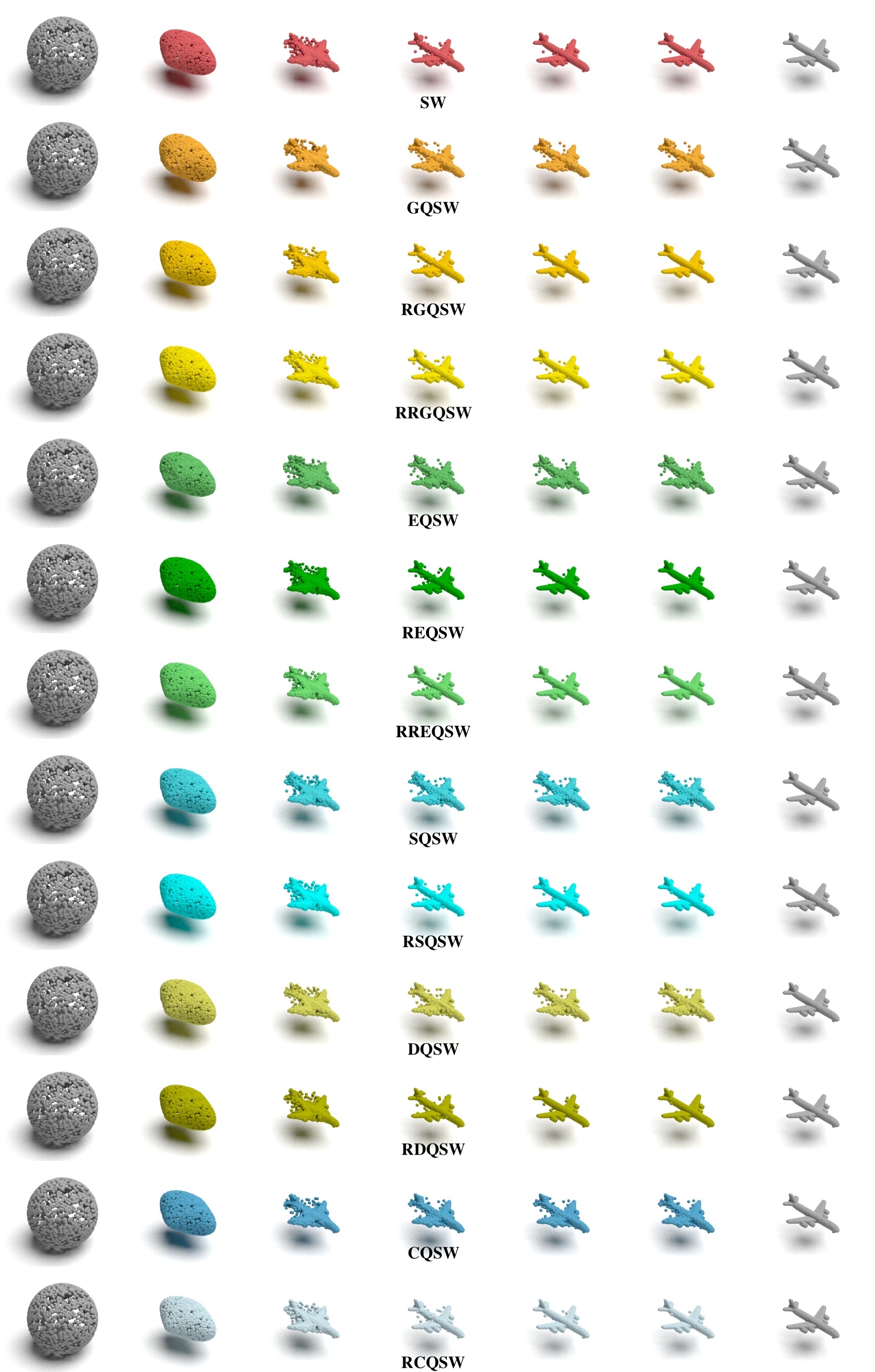
Figure 8: Point-cloud interpolation from SW, QSW variants, and RQSW variants with $L=100$.

Results for $L=10$. We repeated the same experiments with $L=10$. We have reported the Wasserstein-2 distances for intermediate point-clouds (relative to the target point-cloud) in Table 3. We observed a similar phenomenon as with $L=100$, namely, RQSW outperforms QSW significantly and also performs better than SW. Compared to $L=100$, all approximations from $L=10$ yield higher Wasserstein-2 distances. However, the gaps between QSW variants are wider. Therefore, RQSW variants are more robust to the choice of $L$ than QSW.

Table 3: Summary of Wasserstein-2 distances (multiplied by $10^{2}$) from three different runs.

Estimators	Step 100 ($\text{W}_{2}\downarrow$)	Step 200 ($\text{W}_{2}\downarrow$)	Step 300 ($\text{W}_{2}\downarrow$)	Step 400($\text{W}_{2}\downarrow$)	Step 500 ($\text{W}_{2}\downarrow$)
SW L=10	$5.821\pm 0.149$	$0.203\pm 0.012$	$0.038\pm 0.002$	$0.017\pm 0.001$	$0.009\pm 0.0$
GQSW L=10	$9.274\pm 0.0$	$3.776\pm 0.0$	$2.572\pm 0.0$	$2.297\pm 0.0$	$2.23\pm 0.0$
EQSW L=10	$\mathbf{4.066\pm 0.0}$	$0.575\pm 0.0$	$0.511\pm 0.0$	$0.508\pm 0.0$	$0.508\pm 0.0$
SQSW L=10	$6.321\pm 0.0$	$1.093\pm 0.0$	$0.603\pm 0.0$	$0.559\pm 0.0$	$0.554\pm 0.0$
DQSW L=10	$5.919\pm 0.0$	$0.87\pm 0.0$	$0.607\pm 0.0$	$0.593\pm 0.0$	$0.593\pm 0.0$
CQSW L=10	$5.561\pm 0.0$	$0.793\pm 0.0$	$0.614\pm 0.0$	$0.606\pm 0.0$	$0.606\pm 0.0$
RGQSW L=10	$5.863\pm 0.029$	$\mathbf{0.188\pm 0.007}$	$0.035\pm 0.002$	$0.018\pm 0.001$	$0.01\pm 0.001$
RRGQSW L=10	$5.781\pm 0.102$	$0.232\pm 0.031$	$0.047\pm 0.002$	$0.03\pm 0.002$	$0.026\pm 0.001$
REQSW L=10	$5.733\pm 0.19$	$0.19\pm 0.014$	$\mathbf{0.034\pm 0.003}$	$0.016\pm 0.002$	$0.008\pm 0.002$
RREQSW L=10	$5.857\pm 0.058$	$0.219\pm 0.007$	$0.042\pm 0.001$	$0.022\pm 0.001$	$0.014\pm 0.001$
RSQSW L=10	$5.754\pm 0.028$	$0.195\pm 0.004$	$0.035\pm 0.002$	$0.016\pm 0.002$	$\mathbf{0.007\pm 0.001}$
RDQSW L=10	$5.835\pm 0.071$	$0.202\pm 0.011$	$0.036\pm 0.002$	$\mathbf{0.016\pm 0.001}$	$0.008\pm 0.001$
RCQSW L=10	$5.794\pm 0.076$	$0.196\pm 0.008$	$0.037\pm 0.003$	$0.017\pm 0.002$	$0.008\pm 0.001$

Results for a different pair of point-clouds. We conduct the same experiments with a different pair of point-clouds, namely, 2 and 3 in Figure 2. We present a summary of Wasserstein-2 distances in Table 4 for $L=100$ and Table 5 for $L=10$. We observe the same phenomena as in the previous experiments. Firstly, RQSW variants produce shorter curves than QSW variants. Secondly, a larger number of projections is better, and RQSW variants are more robust to changes in $L$ than QSW variants. Additionally, we provide visualizations for $L=100$ in Figure 9. From the figure, we can see consistent qualitative comparisons with the Wasserstein-2 distances reported in the tables.

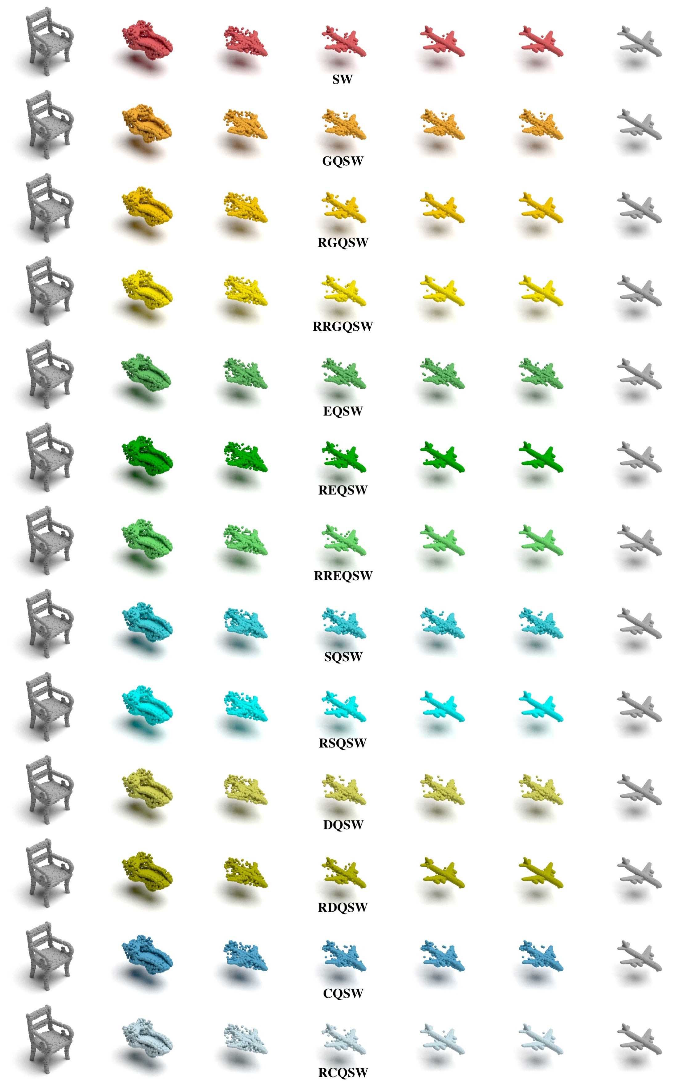
Figure 9: Point-cloud interpolation from SW, QSW variants, and RQSW variants with $L=100$.

Table 4: Summary of Wasserstein-2 distances (multiplied by $10^{2}$) from three different runs.

Estimators	Step 100 ($\text{W}_{2}\downarrow$)	Step 200 ($\text{W}_{2}\downarrow$)	Step 300 ($\text{W}_{2}\downarrow$)	Step 400($\text{W}_{2}\downarrow$)	Step 500 ($\text{W}_{2}\downarrow$)
SW L=100	$2.819\pm 0.044$	$0.23\pm 0.002$	$0.033\pm 0.002$	$0.012\pm 0.002$	$0.006\pm 0.001$
GQSW L=100	$2.868\pm 0.0$	$0.281\pm 0.0$	$0.107\pm 0.0$	$0.093\pm 0.0$	$0.091\pm 0.0$
EQSW L=100	$\mathbf{2.473\pm 0.0}$	$0.229\pm 0.0$	$0.109\pm 0.0$	$0.1\pm 0.0$	$0.098\pm 0.0$
SQSW L=100	$2.841\pm 0.0$	$0.262\pm 0.0$	$0.109\pm 0.0$	$0.098\pm 0.0$	$0.096\pm 0.0$
DQSW L=100	$2.883\pm 0.0$	$0.262\pm 0.0$	$0.101\pm 0.0$	$0.093\pm 0.0$	$0.091\pm 0.0$
CQSW L=100	$2.696\pm 0.0$	$0.223\pm 0.0$	$0.092\pm 0.0$	$0.085\pm 0.0$	$0.084\pm 0.0$
RGQSW L=100	$2.815\pm 0.017$	$0.231\pm 0.005$	$0.031\pm 0.001$	$0.01\pm 0.001$	$0.004\pm 0.001$
RRGQSW L=100	$2.82\pm 0.044$	$0.233\pm 0.008$	$0.034\pm 0.002$	$0.013\pm 0.002$	$0.006\pm 0.002$
REQSW L=100	$2.826\pm 0.006$	$0.229\pm 0.002$	$0.03\pm 0.001$	$0.01\pm 0.0$	$0.004\pm 0.0$
RREQSW L=100	$2.83\pm 0.015$	$0.23\pm 0.002$	$0.031\pm 0.001$	$0.011\pm 0.0$	$0.005\pm 0.001$
RSQSW L=100	$2.796\pm 0.003$	$\mathbf{0.224\pm 0.001}$	$0.028\pm 0.002$	$0.008\pm 0.001$	$0.003\pm 0.0$
RDQSW L=100	$2.793\pm 0.002$	$\mathbf{0.224\pm 0.001}$	$\mathbf{0.028\pm 0.001}$	$\mathbf{0.008\pm 0.001}$	$\mathbf{0.002\pm 0.0}$
RCQSW L=100	$2.794\pm 0.005$	$0.227\pm 0.002$	$0.03\pm 0.001$	$0.01\pm 0.002$	$0.005\pm 0.002$

Table 5: Summary of Wasserstein-2 distances (multiplied by $10^{2}$) from three different runs.

Estimators	Step 100 ($\text{W}_{2}\downarrow$)	Step 200 ($\text{W}_{2}\downarrow$)	Step 300 ($\text{W}_{2}\downarrow$)	Step 400($\text{W}_{2}\downarrow$)	Step 500 ($\text{W}_{2}\downarrow$)
SW L=10	$2.919\pm 0.082$	$0.262\pm 0.018$	$0.048\pm 0.007$	$0.02\pm 0.004$	$0.01\pm 0.003$
GQSW L=10	$6.576\pm 0.0$	$2.863\pm 0.0$	$2.305\pm 0.0$	$2.197\pm 0.0$	$2.165\pm 0.0$
EQSW L=10	$2.391\pm 0.0$	$0.789\pm 0.0$	$0.617\pm 0.0$	$0.6\pm 0.0$	$0.6\pm 0.0$
SQSW L=10	$3.498\pm 0.0$	$1.437\pm 0.0$	$0.87\pm 0.0$	$0.783\pm 0.0$	$0.776\pm 0.0$
DQSW L=10	$2.9\pm 0.0$	$1.118\pm 0.0$	$0.796\pm 0.0$	$0.754\pm 0.0$	$0.746\pm 0.0$
CQSW L=10	$3.465\pm 0.0$	$1.596\pm 0.0$	$1.129\pm 0.0$	$1.035\pm 0.0$	$1.027\pm 0.0$
RGQSW L=10	$2.979\pm 0.048$	$0.266\pm 0.007$	$0.045\pm 0.002$	$0.019\pm 0.001$	$0.009\pm 0.001$
RRGQSW L=10	$2.928\pm 0.056$	$0.271\pm 0.021$	$0.051\pm 0.003$	$0.028\pm 0.002$	$0.022\pm 0.001$
REQSW L=10	$2.891\pm 0.089$	$0.25\pm 0.013$	$0.045\pm 0.002$	$0.02\pm 0.001$	$0.01\pm 0.001$
RREQSW L=10	$2.907\pm 0.103$	$0.268\pm 0.011$	$0.055\pm 0.003$	$0.027\pm 0.002$	$0.017\pm 0.001$
RSQSW L=10	$\mathbf{2.747\pm 0.006}$	$0.24\pm 0.002$	$0.047\pm 0.0$	$0.02\pm 0.001$	$0.01\pm 0.002$
RDQSW L=10	$2.769\pm 0.015$	$\mathbf{0.239\pm 0.008}$	$0.044\pm 0.004$	$0.019\pm 0.004$	$0.009\pm 0.002$
RCQSW L=10	$2.761\pm 0.101$	$0.241\pm 0.009$	$\mathbf{0.043\pm 0.0}$	$\mathbf{0.018\pm 0.002}$	$\mathbf{0.009\pm 0.001}$

Recommended variants. Overall, we recommend RSQSW, RDQSW, and RCQSW for the point-cloud interpolation application since they give consistent performance for $L=100$ and $L=10$ for both tried pairs of point-clouds.

D.3 Image Style Transfer

Detailed settings. We first reduce the number of colors in the images to 3000 using K-means clustering. Similar to the point-cloud interpolation, we iterate through the curve between the empirical distribution of colors in the source image and the empirical distribution of colors in the target image using the approximate Euler method.

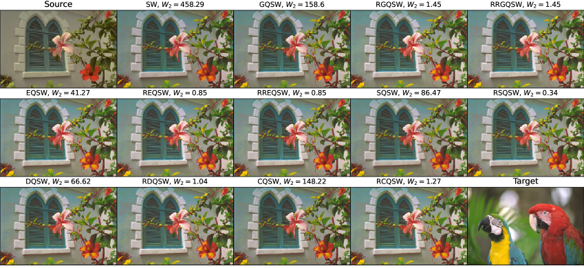
Figure 10: Style-transferred images from SW, QSW variants, and RQSW variants with $L=100$.

Full results for $L=100$. We present style-transferred images and their corresponding Wasserstein-2 distances to the target image in terms of color palettes at the last iteration (1000) in Figure 10. From the figure, it is evident that QSW variants facilitate faster color transfer compared to SW. To elaborate, SW exhibits a Wasserstein-2 distance of 458.29, while the highest Wasserstein-2 distance among QSW variants is 158.6, achieved by GQSW. The use of RQSW can further enhance quality; for instance, the highest Wasserstein-2 distance among RQSW variants is 1.45, achieved by RGQSW. The best-performing variant in this application is RSQSW; however, other RQSW variants are also comparable.

Full results for $L=10$. We repeat the experiment with $L=10$. In all approximations, decreasing $L$ to 10 results in a higher Wasserstein-2 distance, which is understandable based on the approximation error analysis. In this scenario, the performance of some QSW variants (GQSW, EBQSW, SQSW) degrades to the point of being even worse than SW. In contrast, the degradation of RQSW variants is negligible, particularly for RCQSW.

Recommended variants. Overall, we recommend RCQSW for this application since it performs consistently for both setting of $L=100$ and $L=10$.

D.4 Deep Point-cloud Autoencoder

Full visualization for $L=100$. We first visualize reconstructed point-clouds from all approximations, including SW, QSW variants, and RQSW variants in Figure 12. Overall, we observe that the sharpness of the reconstructed point-clouds aligns with the reconstruction losses presented in Table 2. However, the point-clouds generated by GQSW lack meaningful structure, likely due to numerical issues encountered during training. These issues may stem from the numerical computation of the inverse CDF for specific projecting directions at certain iterations. Randomized versions of GQSW could potentially mitigate such problems, as stochastic gradient training may help avoid undesirable configurations in neural networks.

Table 6: Reconstruction errors (multiplied by 100) from three different runs of autoencoders trained by different approximations of SW with L=10.

Distance	Epoch 100		Epoch 200		Epoch 400
	$\text{SW}_{2}$($\downarrow$)	$\text{W}_{2}$($\downarrow$)	$\text{SW}_{2}$ ($\downarrow$)	$\text{W}_{2}$($\downarrow$)	$\text{SW}_{2}$ ($\downarrow$)	$\text{W}_{2}$($\downarrow$)
SW L=10	$2.27\pm 0.05$	$10.60\pm 0.10$	$2.12\pm 0.04$	$9.93\pm 0.02$	$1.95\pm 0.06$	$9.24\pm 0.09$
GQSW L=10	$11.18\pm 0.06$	$32.64\pm 0.06$	$11.78\pm 0.07$	$33.35\pm 0.07$	$14.85\pm 0.03$	$38.04\pm 0.04$
EQSW L=10	$2.53\pm 0.07$	$11.82\pm 0.12$	$2.29\pm 0.02$	$11.03\pm 0.05$	$2.11\pm 0.03$	$10.40\pm 0.03$
SQSW L=10	$2.46\pm 0.04$	$11.55\pm 0.07$	$2.23\pm 0.05$	$10.82\pm 0.05$	$2.05\pm 0.06$	$10.15\pm 0.01$
DQSW L=10	$3.10\pm 0.03$	$12.89\pm 0.04$	$2.86\pm 0.07$	$12.17\pm 0.10$	$2.56\pm 0.03$	$11.33\pm 0.08$
CQSW L=10	$2.60\pm 0.04$	$11.92\pm 0.02$	$2.44\pm 0.03$	$11.29\pm 0.07$	$2.25\pm 0.10$	$10.59\pm 0.13$
RGQSW L=10	$2.27\pm 0.05$	$10.60\pm 0.06$	$2.10\pm 0.05$	$9.92\pm 0.09$	$1.95\pm 0.03$	$9.20\pm 0.03$
RRGQSW L=10	$2.26\pm 0.02$	$10.58\pm 0.03$	$2.06\pm 0.08$	$9.85\pm 0.12$	$1.89\pm 0.06$	$9.18\pm 0.07$
REQSW L=10	$2.26\pm 0.06$	$10.57\pm 0.05$	$2.09\pm 0.05$	$9.91\pm 0.05$	$1.91\pm 0.01$	$9.20\pm 0.03$
RREQSW L=10	$2.24\pm 0.03$	$10.54\pm 0.06$	$2.06\pm 0.03$	$9.85\pm 0.04$	$1.88\pm 0.07$	$9.17\pm 0.10$
RSQSW L=10	$\mathbf{2.23\pm 0.05}$	$10.54\pm 0.08$	$2.05\pm 0.03$	$9.83\pm 0.03$	$\mathbf{1.86\pm 0.03}$	$9.14\pm 0.02$
RDQSW L=10	$2.24\pm 0.03$	$\mathbf{10.54\pm 0.06}$	$2.05\pm 0.03$	$9.85\pm 0.04$	$1.87\pm 0.03$	$9.14\pm 0.02$
RCQSW L=10	$2.24\pm 0.04$	$10.55\pm 0.03$	$\mathbf{2.03\pm 0.03}$	$\mathbf{9.83\pm 0.03}$	$1.87\pm 0.02$	$\mathbf{9.13\pm 0.06}$

Results for $L=10$. We reduce the number of projections $L$ to 10 and subsequently report the reconstruction losses in Table 6. Similar to other applications, reducing $L$ results in increased reconstruction losses, particularly for QSW variants. In this specific application, RQSW variants demonstrate their robustness to the choice of $L$; the reconstruction losses for $L=10$ are comparable to those for $L=100$, as shown in Table 2. Additionally, we provide visualizations of the reconstructed point-clouds for $L=10$ in Figure 13. It is evident from the figure that reconstructed point-clouds from QSW variants exhibit significant noise.

Recommended variants. Overall, we recommend RCQSW for this application since it performs well in both settings of $L=100$ and $L=10$ in terms of both reconstruction losses and qualitative comparison.

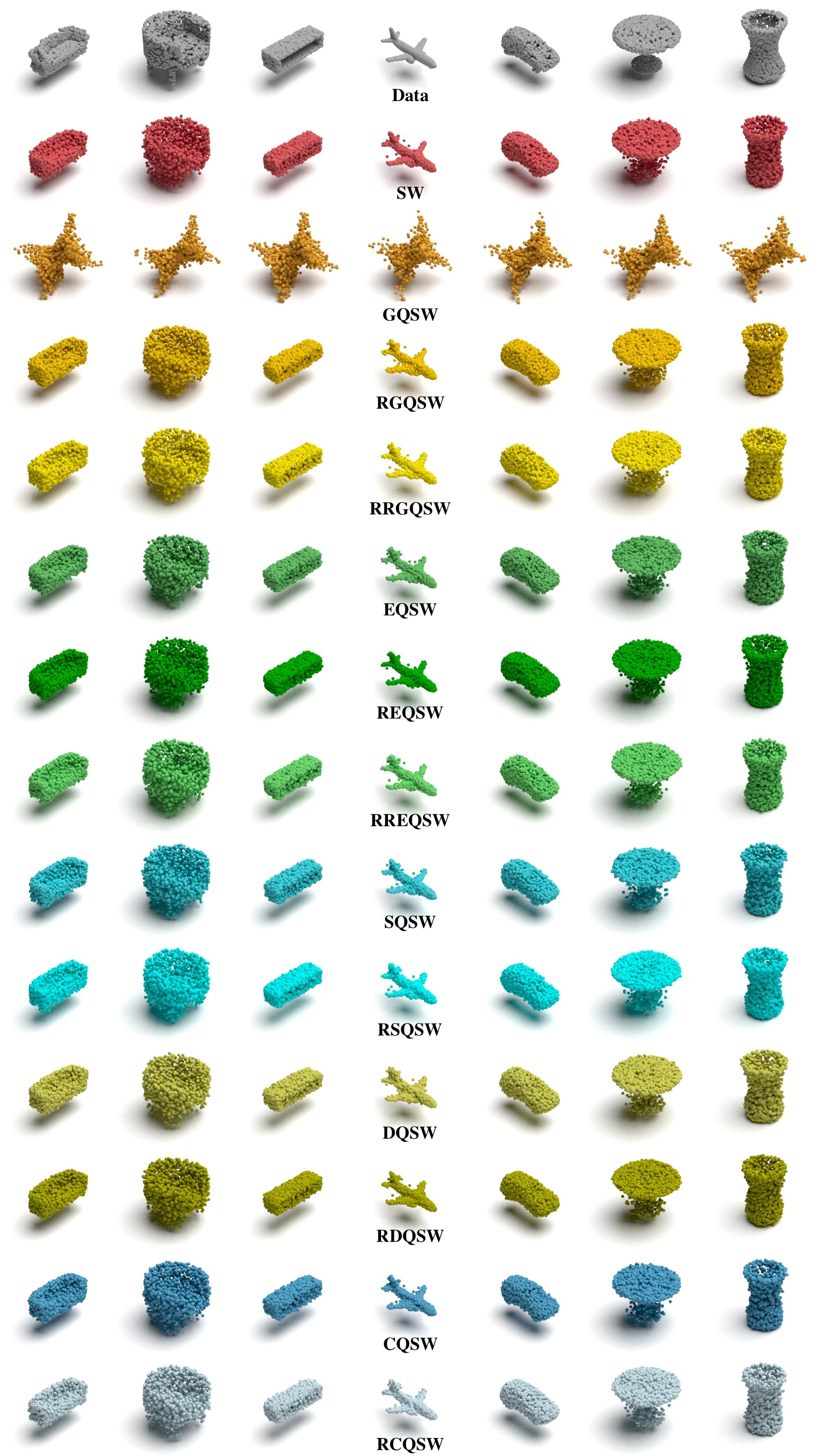
Figure 12: Some reconstructed point-clouds from SW, QSW variants, and RQSW variants with $L=100$.

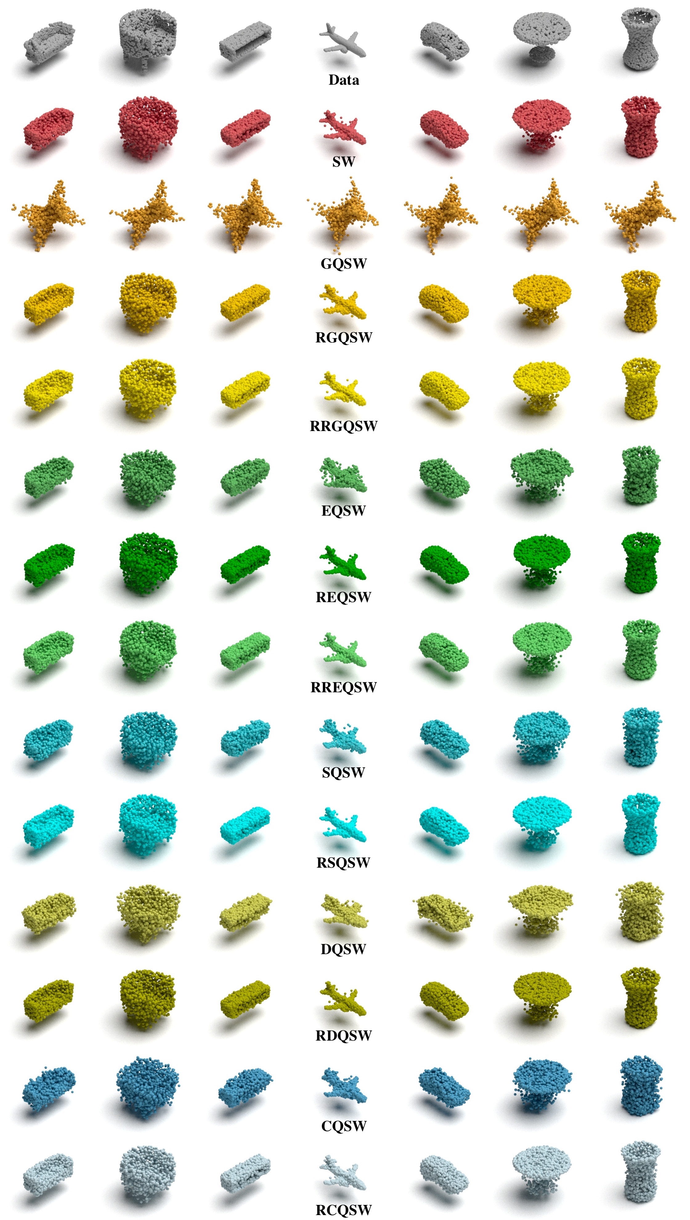
Figure 13: Some reconstructed point-clouds from SW, QSW variants, and RQSW variants with $L=10$.

Appendix E Computational Infrastructure

We use a single NVIDIA V100 GPU to conduct experiments on training deep point-cloud autoencoder. Other applications are done on a desktop with an Intel core I5 CPU chip.

References

- [1] P. Achlioptas, O. Diamanti, I. Mitliagkas, and L. Guibas. Learning representations and generative models for 3d point clouds. In International conference on machine learning, pages 40–49. PMLR, 2018.
- [2] C. Aistleitner, J. S. Brauchart, and J. Dick. Point sets on the sphere with small spherical cap discrepancy. Discrete & Computational Geometry, 48(4):990–1024, 2012.
- [3] B. Amos, S. Cohen, G. Luise, and I. Redko. Meta optimal transport. International Conference on Machine Learning, 2023.
- [4] K. Basu. Quasi-Monte Carlo Methods in Non-Cubical Spaces. Stanford University, 2016.
- [5] C. Bonet, N. Courty, F. Septier, and L. Drumetz. Efficient gradient flows in sliced-Wasserstein space. Transactions on Machine Learning Research, 2022.
- [6] N. Bonneel, J. Rabin, G. Peyré, and H. Pfister. Sliced and Radon Wasserstein barycenters of measures. Journal of Mathematical Imaging and Vision, 1(51):22–45, 2015.
- [7] J. Brauchart, E. Saff, I. Sloan, and R. Womersley. Qmc designs: optimal order quasi monte carlo integration schemes on the sphere. Mathematics of computation, 83(290):2821–2851, 2014.
- [8] J. S. Brauchart and J. Dick. Quasi–monte carlo rules for numerical integration over the unit sphere. Numerische Mathematik, 121(3):473–502, 2012.
- [9] A. X. Chang, T. Funkhouser, L. Guibas, P. Hanrahan, Q. Huang, Z. Li, S. Savarese, M. Savva, S. Song, H. Su, et al. Shapenet: An information-rich 3d model repository. arXiv preprint arXiv:1512.03012, 2015.
- [10] N. Courty, R. Flamary, A. Habrard, and A. Rakotomamonjy. Joint distribution optimal transportation for domain adaptation. In Advances in Neural Information Processing Systems, pages 3730–3739, 2017.
- [11] R. Cranley and T. N. Patterson. Randomization of number theoretic methods for multiple integration. SIAM Journal on Numerical Analysis, 13(6):904–914, 1976.
- [12] H. Faure. Discrépance de suites associées à un système de numération (en dimension s). Acta arithmetica, 41(4):337–351, 1982.
- [13] J. Feydy, B. Charlier, F.-X. Vialard, and G. Peyré. Optimal transport for diffeomorphic registration. In Medical Image Computing and Computer Assisted Intervention- MICCAI 2017: 20th International Conference, Quebec City, QC, Canada, September 11-13, 2017, Proceedings, Part I 20, pages 291–299. Springer, 2017.
- [14] R. Flamary, N. Courty, A. Gramfort, M. Z. Alaya, A. Boisbunon, S. Chambon, L. Chapel, A. Corenflos, K. Fatras, N. Fournier, L. Gautheron, N. T. Gayraud, H. Janati, A. Rakotomamonjy, I. Redko, A. Rolet, A. Schutz, V. Seguy, D. J. Sutherland, R. Tavenard, A. Tong, and T. Vayer. Pot: Python optimal transport. Journal of Machine Learning Research, 22(78):1–8, 2021.
- [15] M. Götz. On the distribution of weighted extremal points on a surface in. Potential Analysis, 13(4):345–359, 2000.
- [16] J. Halton and G. Smith. Radical inverse quasi-random point sequence, algorithm 247. Commun. ACM, 7(12):701, 1964.
- [17] J. Hammersley. Monte carlo methods. Springer Science & Business Media, 2013.
- [18] D. P. Hardin, T. Michaels, and E. B. Saff. A comparison of popular point configurations on . arXiv preprint arXiv:1607.04590, 2016.
- [19] H. Heitsch and R. Henrion. An enumerative formula for the spherical cap discrepancy. Journal of Computational and Applied Mathematics, 390:113409, 2021.
- [20] E. Heitz, K. Vanhoey, T. Chambon, and L. Belcour. A sliced Wasserstein loss for neural texture synthesis. In Proceedings of the IEEE/CVF Conference on Computer Vision and Pattern Recognition, pages 9412–9420, 2021.
- [21] E. Hlawka. Funktionen von beschränkter variatiou in der theorie der gleichverteilung. Annali di Matematica Pura ed Applicata, 54(1):325–333, 1961.
- [22] N. Ho, X. Nguyen, M. Yurochkin, H. H. Bui, V. Huynh, and D. Phung. Multilevel clustering via Wasserstein means. In International Conference on Machine Learning, pages 1501–1509, 2017.
- [23] T. Huang, Z. Ding, J. Zhang, Y. Tai, Z. Zhang, M. Chen, C. Wang, and Y. Liu. Learning to measure the point cloud reconstruction loss in a representation space. In Proceedings of the IEEE/CVF Conference on Computer Vision and Pattern Recognition, pages 12208–12217, 2023.
- [24] S. Joe and F. Y. Kuo. Remark on algorithm 659: Implementing Sobol’s quasirandom sequence generator. ACM Transactions on Mathematical Software (TOMS), 29(1):49–57, 2003.
- [25] A. Keller. A quasi-monte carlo algorithm for the global illumination problem in the radiosity setting. In Monte Carlo and Quasi-Monte Carlo Methods in Scientific Computing: Proceedings of a conference at the University of Nevada, Las Vegas, Nevada, USA, June 23–25, 1994, pages 239–251. Springer, 1995.
- [26] H. Kim, H. Lee, W. H. Kang, J. Y. Lee, and N. S. Kim. Softflow: Probabilistic framework for normalizing flow on manifolds. Advances in Neural Information Processing Systems, 33:16388–16397, 2020.
- [27] J. Koksma. Een algemeene stelling uit de theorie der gelijkmatige verdeeling modulo 1. Mathematica B (Zutphen), 11(7-11):43, 1942.
- [28] S. Kolouri, G. K. Rohde, and H. Hoffmann. Sliced Wasserstein distance for learning Gaussian mixture models. In Proceedings of the IEEE Conference on Computer Vision and Pattern Recognition, pages 3427–3436, 2018.
- [29] R. Lai and H. Zhao. Multiscale nonrigid point cloud registration using rotation-invariant sliced-Wasserstein distance via laplace–beltrami eigenmap. SIAM Journal on Imaging Sciences, 10(2):449–483, 2017.
- [30] T. Le, K. Nguyen, S. Sun, K. Han, N. Ho, and X. Xie. Diffeomorphic deformation via sliced Wasserstein distance optimization for cortical surface reconstruction. arXiv preprint arXiv:2305.17555, 2023.
- [31] C.-Y. Lee, T. Batra, M. H. Baig, and D. Ulbricht. Sliced Wasserstein discrepancy for unsupervised domain adaptation. In Proceedings of the IEEE/CVF Conference on Computer Vision and Pattern Recognition, pages 10285–10295, 2019.
- [32] T. Li, C. Meng, J. Yu, and H. Xu. Hilbert curve projection distance for distribution comparison. arXiv preprint arXiv:2205.15059, 2022.
- [33] H. Lin, H. Chen, K. M. Choromanski, T. Zhang, and C. Laroche. Demystifying orthogonal monte carlo and beyond. Advances in Neural Information Processing Systems, 33:8030–8041, 2020.
- [34] P. Mattila. Geometry of sets and measures in Euclidean spaces: fractals and rectifiability. Number 44. Cambridge university press, 1999.
- [35] R. J. Muirhead. Aspects of multivariate statistical theory. John Wiley & Sons, 2009.
- [36] K. Nadjahi, A. Durmus, L. Chizat, S. Kolouri, S. Shahrampour, and U. Simsekli. Statistical and topological properties of sliced probability divergences. Advances in Neural Information Processing Systems, 33:20802–20812, 2020.
- [37] K. Nguyen and N. Ho. Control variate sliced Wasserstein estimators. arXiv preprint arXiv:2305.00402, 2023.
- [38] K. Nguyen and N. Ho. Energy-based sliced Wasserstein distance. arXiv preprint arXiv:2304.13586, 2023.
- [39] K. Nguyen, N. Ho, T. Pham, and H. Bui. Distributional sliced-Wasserstein and applications to generative modeling. In International Conference on Learning Representations, 2021.
- [40] K. Nguyen, D. Nguyen, and N. Ho. Self-attention amortized distributional projection optimization for sliced Wasserstein point-cloud reconstruction. Proceedings of the 40th International Conference on Machine Learning, 2023.
- [41] H. Niederreiter. Random number generation and quasi-Monte Carlo methods. SIAM, 1992.
- [42] A. B. Owen. Randomly permuted (t, m, s)-nets and (t, s)-sequences. In Monte Carlo and Quasi-Monte Carlo Methods in Scientific Computing: Proceedings of a conference at the University of Nevada, Las Vegas, Nevada, USA, June 23–25, 1994, pages 299–317. Springer, 1995.
- [43] A. B. Owen. Monte carlo theory, methods and examples. 2013.
- [44] L. Paulin, N. Bonneel, D. Coeurjolly, J.-C. Iehl, A. Webanck, M. Desbrun, and V. Ostromoukhov. Sliced optimal transport sampling. ACM Trans. Graph., 39(4):99, 2020.
- [45] G. Peyré and M. Cuturi. Computational optimal transport: With applications to data science. Foundations and Trends® in Machine Learning, 11(5-6):355–607, 2019.
- [46] G. Peyré and M. Cuturi. Computational optimal transport, 2020.
- [47] C. R. Qi, H. Su, K. Mo, and L. J. Guibas. Pointnet: Deep learning on point sets for 3d classification and segmentation. In Proceedings of the IEEE conference on computer vision and pattern recognition, pages 652–660, 2017.
- [48] E. A. Rakhmanov, E. B. Saff, and Y. Zhou. Minimal discrete energy on the sphere. Mathematical Research Letters, 1(6):647–662, 1994.
- [49] T. Salimans, H. Zhang, A. Radford, and D. Metaxas. Improving GANs using optimal transport. In International Conference on Learning Representations, 2018.
- [50] A. Savkin, Y. Wang, S. Wirkert, N. Navab, and F. Tombari. Lidar upsampling with sliced Wasserstein distance. IEEE Robotics and Automation Letters, 8(1):392–399, 2022.
- [51] Z. Shen, J. Feydy, P. Liu, A. H. Curiale, R. San Jose Estepar, R. San Jose Estepar, and M. Niethammer. Accurate point cloud registration with robust optimal transport. Advances in Neural Information Processing Systems, 34:5373–5389, 2021.
- [52] I. Sobol. The distribution of points in a cube and the accurate evaluation of integrals (in russian) zh. Vychisl. Mat. i Mater. Phys, 7:784–802, 1967.
- [53] E. Tanguy. Convergence of sgd for training neural networks with sliced Wasserstein losses. arXiv preprint arXiv:2307.11714, 2023.
- [54] C. Villani. Optimal transport: Old and New. Springer, 2008.
- [55] Z. Wu, S. Song, A. Khosla, F. Yu, L. Zhang, X. Tang, and J. Xiao. 3d shapenets: A deep representation for volumetric shapes. In Proceedings of the IEEE conference on computer vision and pattern recognition, pages 1912–1920, 2015.
- [56] M. Yi and S. Liu. Sliced Wasserstein variational inference. In Fourth Symposium on Advances in Approximate Bayesian Inference, 2021.
Supplement to “Quasi-Monte Carlo for 3D Sliced Wasserstein"
We first provide proofs for theoretical results in the main text in Appendix A. Next, we offer additional background information, including the Wasserstein distance, and computational algorithms for SW, QSW, and RQSW in Appendix B. We then discuss related works in Appendix C. Afterward, we present detailed experimental results, which are mentioned in the main text for point-cloud interpolation, image style transfer, and deep point-cloud autoencoder in Appendix D. Finally, we report the computational infrastructure in Appendix E