MoDA: Leveraging Motion Priors from Videos for Advancing Unsupervised Domain Adaptation in Semantic Segmentation

Abstract

Unsupervised domain adaptation (UDA) is an effective approach to handle the lack of annotations in the target domain for the semantic segmentation task. In this work, we consider a more practical UDA setting where the target domain contains sequential frames of the unlabeled videos which are easy to collect in practice. A recent study suggests self-supervised learning of the object motion from unlabeled videos with geometric constraints. We design a motion-guided domain adaptive semantic segmentation framework (MoDA), that utilizes self-supervised object motion to learn effective representations in the target domain. MoDA differs from previous methods that use temporal consistency regularization for the target domain frames. Instead, MoDA deals separately with the domain alignment on the foreground and background categories using different strategies. Specifically, MoDA contains foreground object discovery and foreground semantic mining to align the foreground domain gaps by taking the instance-level guidance from the object motion. Additionally, MoDA includes background adversarial training which contains a background category-specific discriminator to handle the background domain gaps. Experimental results on multiple benchmarks highlight the effectiveness of MoDA against existing approaches in the domain adaptive image segmentation and domain adaptive video segmentation. Moreover, MoDA is versatile and can be used in conjunction with existing state-of-the-art approaches to further improve performance.

I Introduction

Fully-supervised semantic segmentation [1, 2] is a data-hungry task requiring all training images’ pixels to be assigned with a semantic label. However, annotating a dataset collected from real-world scenes [3] is expensive and time-consuming since human operators must manually label all pixels. Recent advancements in computer graphics have provided new solutions for the semantic segmentation community. For example, with synthesized rendering pipelines, we can quickly generate a labeled virtual dataset, such as GTA5 [4] and SYNTHIA [5] (called the source domain). To bridge the gap between the simulated and real scenes (called the target domain), domain adaptation techniques address domain shift or distribution change. This scenario is called unsupervised domain adaptation (UDA) because no labels are provided in the target domain.

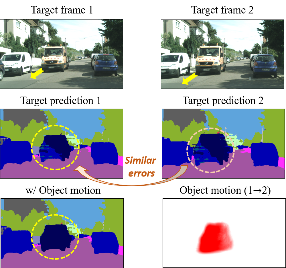
Figure 1: We propose to use the object motion as complementary guidance for domain adaptation in semantic segmentation. This is different from temporal consistency regularization which cannot handle similar errors on the sequential target frames. The object motion is predicted by self-supervised learning from unlabeled target video frames with geometric constraints.

Current UDA methods [6, 7, 8, 9, 10, 11, 12] for semantic segmentation assume that the target domain comprises non-sequential images. Specifically, they adopt Cityscapes [3] with unlabeled 2,975 non-sequential images as the target domain. However, we assume the sequential video frames are accessible in the target domain; One can easily collect a set of sequential video frames in a real scene. In this work, we consider a more practical UDA setting where the target domain consists of unlabeled sequential image pairs, with each pair consisting of an image and its adjacent frame, and the source domain follows the same setting as existing UDA approaches [6, 13, 9, 7, 14]. Under this setting, one method for domain alignment is to leverage the consistency across the sequential image pairs, as proposed in [15]. [15] involves computing the optical flows between the sequential image pairs in the target domain and using them to warp the predictions from its sequential pair onto the current image. Based on this, the temporal consistency for the predictions made on the two images is established. However, using optical flow alone leads to limited performance gain as it fails in addressing similar prediction errors in sequential image pairs of the same object in the target domain, as shown in the truck in Fig. 1.

The recent trend in dynamic scene understanding involves learning the object motion and the camera’s ego-motion from unlabeled sequential image pairs. Existing works [16, 17, 18] suggest learning a motion network to disentangle the local object motion from the global camera ego-motion in the static scenes with self-supervised geometrical constraints. A bird’s eye view illustration from Fig. 2 (a) shows an example of the object motion and the camera’s ego-motion. This separation helps to isolate the object motion from the camera’s ego-motion. Regardless of the cameras’ ego-motion, the object motion is capable of segmenting the moving objects out from static scenes. We propose that the object motion learned from geometric constraints can be used as complementary guidance to learn effective representations in the target domain. Specifically, the segmentation network suffers from the cross-domain gap due to the lack of semantic labels in the target domain. However, the motion network is trained separately from the segmentation network. Moreover, the motion network is trained only using target frames in the self-supervised manner with geometric constraints (finding temporal correspondence of frames within the target domain), which does not require any semantic labels. So the object motion from the motion network is not affected by the cross-domain gaps caused by the labeling issue.

In this work, we present a motion-guided unsupervised domain adaption (MoDA) method for the semantic segmentation task, which utilizes the self-supervised object motion from geometrical constraints as prior. MoDA divides all the categories into two sets: the foreground categories that can move and the background categories that cannot move. On this basis, MoDA considers foreground and background categories separately for domain alignment using different strategies. To bridge the domain gaps in the foreground categories, MoDA presents two novel and complementary modules, namely foreground object discovery (FOD) and foreground semantic mining (FSM), taking the instance-level guidance from motion to improve the pixel-wise semantic predictions in the target domain. Moreover, MoDA introduces background adversarial training (BAT), which includes a background category-specific discriminator for the domain alignment of the background categories. Experimental results on the benchmark datasets show the effectiveness of MoDA compared with state-of-the-art approaches on both the domain adaptive image segmentation and the domain adaptive video segmentation. Additionally, MoDA is versatile and can be incorporated with existing state-of-the-art approaches, for a further performance boost.

In summary, our contributions are listed as follows:

1. We consider a more practical unsupervised domain adaptation setting where the target domain contains sequential frames of the unlabeled videos which are easy to collect in practice. We apply the object motion learned by the self-supervised motion network based on geometric constraints (without extra labels) for semantic segmentation.

2. We propose a motion-guided domain adaptation (MoDA) method using the self-supervised object motion learned from geometrical constraints for semantic segmentation. MoDA handles the domain gaps in the foreground and background categories with different adaptation guidance. Specifically, MoDA contains FOD and FSM to align the foreground categories by taking the instance-level guidance from the self-supervised object motion. Additionally, MoDA includes BAT to reduce the cross-domain discrepancy on the background categories.

3. MoDA shows superior performance on the benchmarks for the domain adaptive image segmentation and the domain adaptive video segmentation. and is complementary to state-of-the-art approaches with various architectures for further performance gain.

II Related Works

Domain adaptive image segmentation. Domain adaptive image segmentation can be regarded as a practical application of transfer learning that leverages labeled data in the source domain to solve problems in a target domain. The goal [19, 20] is to align the domain shift between the labeled source and target domains. In this community, adversarial learning [10, 11, 21, 22, 23] and self-training [7, 14, 24, 25, 26, 9, 27, 28, 29] approaches are widely adopted, and demonstrate compelling adaption results. [21] designs two discriminator networks to implement the inter-domain and intra-domain alignment. [30] proposes to average the predictions from the source and the target domain to stabilize the self-training process and further incorporated the uncertainty [27] to minimize the prediction variance. Existing works consider the domain alignment on the category level [31] and instance level [32] to learn domain-invariant features.  [33] proposes to handle more diverse data in the target domain. adopt image-level annotations from the target domain to bridge the domain gap.  [34] propose combined learning of depth and segmentation for domain adaptation with self-supervision from geometric constraints. Despite the impressive progress, we consider using motion priors as guidance for domain alignment in this work. We deal separately with foreground categories and background categories with different alignment strategies. On this basis, we further deal separately with foreground categories and background categories with different alignment strategies.

Self-training for domain alignment. In self-training, the network is trained with pseudo-labels from the target domain, which can be pre-computed offline or calculated online during training [7, 14, 9, 13, 6].  [7] proposes to estimate category-level prototypes on-the-fly and refine the pseudo labels iteratively, to enhance the adaptation effect. [9] utilizes data augmentation and momentum updates to regulate cross-domain consistency.  [35] proposes to align the cross-domain gaps on structural affinity space for the segmentation task. In this work, we introduce the motion masks that provide complementary object geometric information as prior. Specifically, we develop the motion-guided self-training and the moving object label mining module to refine the target pseudo labels and thus improve the adaptation performance.

Domain adaptive video segmentation. Exploiting motion information like optical flow [36] to separate the objects in videos to regulate the segmentation training is well explored in the video segmentation field. In UDA, there are several attempts that introduce temporal supervision signals to enforce the domain alignment. [37] regulates the cross-domain temporal consistency with adversarial training to minimize the distribution discrepancy. [15] proposes to capture the spatiotemporal consistency in the source domain by data augmentation across frames. In this work, we propose to utilize the 3D object motion  [16] of the target sequential image pairs, which provides rich information for localizing and segmenting the moving objects.

III Preliminary

III-A Notation and Overview

We explore a new setting for UDA in semantic segmentation where the target domain contains sequential image pairs. We have a set of source images $X^{\mathbb{S}}=\{x^{\mathbb{S}}_{n}\}_{n=1}^{N^{\mathbb{S}}}$ with the corresponding segmentation annotations $Y^{\mathbb{S}}=\{y^{\mathbb{S}}\}_{n=1}^{N^{\mathbb{S}}}$, where $N^{\mathbb{S}}$ is the number of the source images. We also have a set of unlabeled sequential image pairs $X^{\mathbb{T}}=\{(x^{\mathbb{T}}_{n,1},x^{\mathbb{T}}_{n,2})\}_{n=1}^{N^{\mathbb{T}}}$ in the target domain, where $x^{\mathbb{T}}_{n,2}$ is an adjacent frame of $x^{\mathbb{T}}_{n,1}$, and $N^{\mathbb{T}}$ is the number of the target image pairs. Note that $x^{\mathbb{T}}\in\mathbb{R}^{H,W,3}$, $x^{\mathbb{S}}\in\mathbb{R}^{\hat{H},\hat{W},3}$, $y^{\mathbb{S}}\in\mathbb{B}^{\hat{H},\hat{W},C}$ as pixel-wise one-hot vectors, and $C$ is the number of all the categories $\mathbb{C}$ . We divide all the categories $\mathbb{C}$ into the foreground categories that can move and the background categories that cannot move . Our objective is to train a cross-domain segmentation model $G$ outputting the pixel-wise softmax prediction over all the categories $\mathbb{C}$ in the target domain. For the geometric part, our motion network and the depth network are represented by $G_{m}$ and $G_{p}$. For the semantic part, our segmentation network is indicated by $G_{e}$. Our objective is to adapt the segmentation model $G_{e}$ onto the unlabeled.

In this section, we first train the motion network $G_{m}$ to learn object motion prediction in the target domain illustrated in Sec. III-B. Then, we conduct motion mask preprocessing to obtain the instance-level motion masks in the target domain shown in Sec. III-C.

III-B Target Domain Geometric Learning

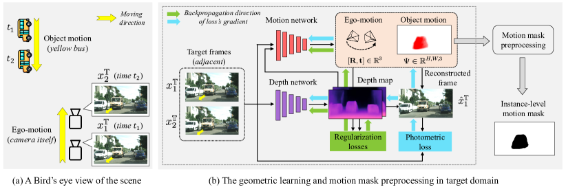
Figure 2: We propose to learn object motion given unlabeled target video frames. (a) is the visualization of a bird’s eye view of the dynamic scene where a yellow bus is moving toward the camera; we visualize the object motion of the yellow bus and the ego motion from the camera itself. (b) shows the diagram for geometric training to learn the object motion from a pair of adjacent frames from the target domain; the motion network and the depth network are trained in a self-supervised manner with geometric constraints; the blue arrows and green arrows represent the gradients directions from the photometric loss and the regularization losses.

The joint acquisition of knowledge concerning the moving objects and the motion of the ego camera within a local static scene has obtained considerable attention within the area of dynamic scene understanding [16, 17, 18, 38]. Recent investigations have introduced a method to disentangle the local objects’ independent motion (called object motion) from the global camera’s motion (called ego-motion) in a self-supervised manner with geometric constraints [16, 17]. A bird’s eye view illustration from Fig. 2 (a) shows an example of the object motion and the camera’s ego-motion. We use the object motion to segment the moving objects out from the static scene.

Given an unlabeled target frame and its adjacent frame $\{x^{\mathbb{T}}_{1},x^{\mathbb{T}}_{2}\}$, our depth network $G_{p}$ is trained to estimate their depth maps $\{d^{\mathbb{T}}_{1},d^{\mathbb{T}}_{2}\}\in\mathbb{R}^{H,W}$. Then these frames with their corresponding depth maps are concatenated as input $\{x^{\mathbb{T}}_{1},d^{\mathbb{T}}_{1},x^{\mathbb{T}}_{2},d^{\mathbb{T}}_{2}\}$ and sent into the motion net $G_{m}$. Then $G_{m}$ is trained generates the camera’s ego-motion $[R,t]$ (in 6 DoF) and the object motion $\Psi\in\mathbb{R}^{H,W,3}$ (in 3D space: $x$, $y$, and $z$-axis), where $R\in\mathbb{R}^{3}$ is the camera’s ego rotation and $t\in\mathbb{R}^{3}$ is the camera’s ego translation. On this basis, we use the camera’s ego-motion $[R,t]$, the object motion $\Psi$, and the adjacent frame $x^{\mathbb{T}}_{2}$ to reconstruct the original image $x^{\mathbb{T}}_{1}$ with an inverse warping operation

$$\hat{x}^{\mathbb{T}}_{1}=\mathcal{F}(x^{\mathbb{T}}_{2},d^{\mathbb{T}}_{1},R,t,\Psi,K),$$ (1)

where $\hat{x}^{\mathbb{T}}_{1}$ is the reconstructed image by warping the adjacent image $x^{\mathbb{T}}_{2}$ (as reference), $\mathcal{F}$ is the projection operation using camera geometry [17], and $K\in\mathbb{R}^{3\times 3}$ is the camera’s intrinsic parameters. We adopt the photometric loss and the regularization losses [16] to optimize the motion network $G_{m}$ and the depth network $G_{p}$ together shown in Fig. 2 (b).

For the photometric loss, we apply the occlusion-aware photometric reconstruction loss $\mathcal{L}_{p}$ which is the sum of the SSIM [39] structural similarity loss and the L1 distance loss.

$$\begin{split}\mathcal{L}_{p}=(1-\text{SSIM}&(x^{\mathbb{T}}_{1},\hat{x}^{\mathbb{T}}_{1}))+\|x^{\mathbb{T}}_{1}-\hat{x}^{\mathbb{T}}_{1}\|_{1}\mathbbm{1}_{{d^{\mathbb{T}}_{1}}_{(u,v)}>{d^{\mathbb{T}}_{1}}_{warp(u,v)}},\end{split}$$ (2)

where $\mathbbm{1}_{{d^{\mathbb{T}}_{1}}_{(u,v)}>{d^{\mathbb{T}}_{1}}_{warp(u,v)}}$ is the occlusion-aware mask introduced by [40]. To generate the desired object motion map $\Psi$ for the moving objects, we adopt two additional losses: the motion smoothness regularization loss $\mathcal{L}_{sm}$ and the motion sparsity regularization loss $\mathcal{L}_{sp}$ defined by

$$\mathcal{L}_{sm}=\sum_{c}\sum_{h,w}\sqrt{(\partial_{h}\Psi^{c})^{2}+(\partial_{w}\Psi^{c})^{2}},$$ (3)

$$\mathcal{L}_{sp}=\sum_{c}2\sigma(\Psi^{c})\sum_{h,w}\sqrt{1+\frac{\Psi^{c}}{\sigma(\Psi^{c})}},$$ (4)

where $\Psi^{c}\in\mathbb{R}^{H,W}$ is the $c\textsuperscript{th}$ channel of $\Psi$ (note that $\Psi$ has 3 channels), and $\sigma(\cdot)$ returns the mean value of the input tensor. Following [16], we also use the depth smoothness regularization loss $\mathcal{L}_{d}$ and the cycle consistency regularization loss $\mathcal{L}_{cy}$ formed by

$$\mathcal{L}_{d}=|\partial_{h}d^{\mathbb{T}}_{1}|e^{-|\partial_{h}x^{\mathbb{T}}_{1}|}+|\partial_{w}d^{\mathbb{T}}_{1}|e^{-|\partial_{w}x^{\mathbb{T}}_{1}|},$$ (5)

$$\mathcal{L}_{yc}=\frac{\|RR^{\prime}-\mathbbm{1}\|^{2}}{\|R-\mathbbm{1}\|^{2}+\|R^{\prime}-\mathbbm{1}\|^{2}}+\frac{\|R^{\prime}t+t^{\prime}\|^{2}}{\|t\|^{2}+\|t^{\prime}\|^{2}},$$ (6)

where $R^{\prime}$ and $t^{\prime}$ are the inverse rotation and the translation of $R$ and $t$. Subsequently, we optimize $G_{m}$ and $G_{p}$ for unsupervised object motion learning through

$$\mathcal{L}=\mathcal{L}_{p}+\mathcal{L}_{sm}+\mathcal{L}_{sp}+\mathcal{L}_{d}+\mathcal{L}_{cy}.$$ (7)

We categorize all the losses into two groups: the photometric loss $\mathcal{L}_{p}$ and the regularization losses $\{\mathcal{L}_{sm},\mathcal{L}_{sp},\mathcal{L}_{d},\mathcal{L}_{cy}\}$. The whole geometric learning process is shown in Fig. 2 (b).

III-C Motion Mask Preprocessing in Target Domain

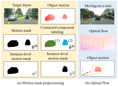
Figure 3: (a) We provide an exemplary procedure for motion mask preprocessing (MMP). (b) The comparison of the optical flow and the object motion while a black car is moving along the $z$-axis in (b); note that the object motion maps here are projected into 2D space from the 3D space for visualization.

Our motion mask preprocessing (MMP) aims at localizing the moving instances based on the object motion information in the target domain. An exemplary procedure of MMP is shown in Fig. 3 (a). Given the motion network $G_{m}$ optimized by the photometric loss and the regularization losses, we first predict the object motion map $\Psi\in\mathbb{R}^{H,W,3}$ from the adjacent frames $x^{\mathbb{T}}_{1},x^{\mathbb{T}}_{2}\in\mathbb{R}^{H,W,3}$ as input. On this basis, we extract a binary motion mask $\Psi^{\mathbb{M}}\in\mathbb{B}^{H,W}$ from $\Psi$ via

$$\Psi^{\mathbb{M}}_{(i)}=\left\{\begin{array}[]{ll}1,&\text{if }|{\Psi}_{(i,d)}|>0,\forall d\in\{1,2,3\}\\ 0,&\text{otherwise}\end{array}\right.,$$ (8)

where $i$ indicate the pixel coordinate, $\Psi^{{}^{\mathbb{M}}}_{(i)}$ is the mask value on the image pixel $x^{\mathbb{T}}_{(i)}$. Note that the object motion $\Psi$ predicted $G_{m}$ is relative to the scene, e.g., it is separated from the camera’s ego-motion. Therefore, we use $\Psi^{\mathbb{M}}$ to localize and segment all the moving objects in the scene.

The binary motion mask $\Psi^{\mathbb{M}}$ could potentially include multiple moving instances, as it is common for multiple cars and motorcycles moving together within the same scenes. To differentiate various moving instances, we utilize a connected component labeling [41] which is to identify each moving instance from $\Psi^{\mathbb{M}}$ with a unique label. The goal of the connected component labeling is to label each connected component (or blob) in the binary image with the same unique label. Because each blob will be labeled, we can infer the total number of individual blobs. Therefore, the connected component labeling helps us to differentiate and identify all the moving instances in the scene. We first run connected component labeling on $\Psi^{\mathbb{M}}$ to get a ”new” map $\tilde{\Psi}^{\mathbb{M}}$ with unique labels

$$\tilde{\Psi}^{\mathbb{M}}=\Gamma(\Psi^{\mathbb{M}}),$$ (9)

where $\Gamma$ is the connected component labeling process [41]. For each unique label $m$ in $\tilde{\Psi}^{\mathbb{M}}$, we extract a binary motion mask $\psi^{m}\in\mathbb{B}^{H,W}$ for the $m\textsuperscript{th}$ moving instance. In this regard, we generate a set of binary instance-level motion masks $\{\psi^{m}\}_{m=1}^{M}$ via

$$\{\psi^{m}\}_{m=1}^{M}=\Delta(\tilde{\Psi}^{\mathbb{M}}),$$ (10)

where $\Delta$ denotes the instance-level motion mask extraction mentioned above (an example is shown in Fig. 3 (a)), and $M$ is the number of the moving instance masks in $\Psi^{\mathbb{M}}$.

The object motion differs from the optical flow in two aspects. First, optical flow is a motion representation in 2D space, it is not accurate for detecting the motion pattern on the front-to-back axis ($z$-axis) which is a common motion pattern in the real world. But such an issue doesn’t exist in object motion which lies in 3D space. Second, the optical flow is a motion representation of all the pixels with respect to the camera’s movement. Therefore, optical flow is a mixed motion representation of the object motion and ego-motion. In contrast, the object motion [16, 17] represents the independent movement of the objects, which is disentangled from the camera’s ego-motion through the learning process in Sec. III-B. Provided a car moving on the $z$-axis, we visualize the optical flow and the object motion in Fig. 3 (b), where the object (black car’s) motion and camera’s ego-motion are similar (toward the $z$-axis with similar velocity). The object motion successfully detects the black car’s motion at the $z$-axis. However, the optical flow cannot easily detect it because the black car’s motion is similar to the camera’s ego-motion.

IV Methodology

IV-A Overview

Initially, we generate the target pseudo labels using the segmentation network optimized with self-training in Sec. IV-B. The target pseudo labels contain noisy predictions on foreground and background categories due to the cross-domain gaps. To handle it, we present a motion-guided domain adaptation (MoDA) framework that aligns the domain gaps of the foreground and background categories separately with different strategies. For foreground category alignment, MoDA contains two newly designed modules, namely foreground object discovery (FOD) in Sec. IV-C and foreground semantic mining (FSM) Sec. IV-D by taking the instance-level moving object masks from Sec. III-C. Moreover, MoDA proposes to align the background categories with adversarial training using a background category-specific discriminator in Sec. IV-E. The overall training process is presented in Sec. IV-F.

IV-B Target Self-training

Given a labeled source frame $x^{\mathbb{S}}$ and its ground-truth map $y^{\mathbb{S}}$, we first train the segmentation network $G_{e}$ with the supervised segmentation loss

$$\mathcal{L}_{ce}^{\mathbb{S}}=-\sum_{i=1}^{\hat{H},\hat{W}}\sum_{c=1}^{C}y_{(i,c)}^{\mathbb{S}}\log(p_{(i,c)}^{\mathbb{S}}),$$ (11)

where the source prediction $p^{\mathbb{S}}=G_{e}(x^{\mathbb{S}})\in\mathbb{R}^{\hat{H},\hat{W},C}$, $p_{(i,c)}^{\mathbb{S}}$ denotes the predicted softmax possibility on $c\textsuperscript{th}$ category on the pixel $x^{\mathbb{S}}_{(i)}$, $G_{e}$ is the segmentation network, and $C$ is the total number of categories. The segmentation network trained solely on the source domain lacks generalization when applied to the target domain. To bridge the domain gap, current self-training methods [26, 9] optimize the cross-entropy loss iteratively with the target pseudo label. For simplicity, let the target pseudo label at the $t\textsuperscript{th}$ iteration denote as $\tilde{y}^{\mathbb{T}}\in\mathbb{B}^{H,W,C}$. The cross-entropy loss is defined by

$$\mathcal{L}_{ce}^{\mathbb{T}}=-\sum_{i=1}^{H,W}\sum_{c=1}^{C}\tilde{y}_{(i,c)}^{\mathbb{T}}\log(p_{(i,c)}^{\mathbb{T}}),$$ (12)

where the target prediction $p^{\mathbb{T}}=G_{e}(x^{\mathbb{T}})\in\mathbb{R}^{H,W,C}$, $p_{(i,c)}^{\mathbb{T}}$ denotes the predicted softmax possibility on $c\textsuperscript{th}$ category on the pixel $x^{\mathbb{T}}_{(i)}$, and $C$ is the total number of categories. We get the target pseudo label $\tilde{y}^{\mathbb{T}}$ using the target prediction $\tilde{p}^{\mathbb{T}}$ via

$$\tilde{y}^{\mathbb{T}}_{(i,c)}=\mathbbm{1}(c=\operatorname*{arg\,max}_{c^{\prime}}\tilde{p}^{\mathbb{T}}_{(i,c^{\prime})}),\forall c\in\mathbb{C},$$ (13)

where $\tilde{p}^{\mathbb{T}}=\tilde{G}_{e}(x^{\mathbb{T}})$ and $\tilde{G}_{e}$ is the momentum network of $G_{e}$. For simplicity, we denote the process of Eq. 13 as $\tilde{y}^{\mathbb{T}}=\Gamma(\tilde{p}^{\mathbb{T}})$, where $\Gamma$ is the operation of taking the most probable category from the softmax probability. Note that the pseudo labels are generated online [26, 9]. $\tilde{G}_{e}$’s network parameters $\tilde{\theta}$ are updated by $G_{e}$’s parameters $\theta$ via exponential moving average (EMA) [42] by $\tilde{\theta}_{t+1}=0.99\tilde{\theta}_{t}+0.01{\theta}_{t}$. Following  [9], we update the momentum network every 100 iterations, and we also adopt color jitter, Gaussian blur, and random flipping as data augmentation to increase the training stability.

IV-C Foreground Object Discovery (FOD) in Target Domain

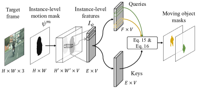
Figure 4: The diagram of foreground object discovery (FOD). Given a target image and its instance-level motion masks, we compute an objectness score map by computing the similarity of each query with all the keys in Eq. 15 and the processing in Eq. 16.

Our goal is to use motion as guidance to improve the quality of the target pseudo labels. However, applying the instance-level motion masks $\{\psi^{m}\}_{m=1}^{M}$ for boosting the quality of target pseudo labels encounters two points of challenge. First, the instance-level motion masks provide a coarse segmentation of the moving objects due to the side effects of the motion regularization loss. Therefore, directly using the instance-level motion masks leads to noisy pseudo labels which might affect the performance of domain alignment. Second, there are some special cases where some moving instances might contain multiple objects. For example, a motorcycle and its rider (two objects) are bounded into one moving instance. We should take these special cases into consideration.

To this end, we propose a self-supervised foreground object discovery (FOD) to learn the accurate moving object masks from the instance-level motion masks $\{\psi^{m}\}_{m=1}^{M}$. The diagram of FOD is shown in Fig. 4. In this step, the segmentation network pre-trained on the source domain (shown in Sec. IV-B) is employed to extract a dense feature map $I\in\mathbb{R}^{H^{\prime},W^{\prime},V}$ given the target frame $x^{\mathbb{T}}$ as input. Then we adopt a self-supervised design to promote the objectness in the features’ attention. Given an instance-level motion mask $\psi^{m}\in\mathbb{B}^{H,W}$ of $x^{\mathbb{T}}$ (generated by Eq. 10), we bilinearly downsample $\psi$ to the spatial size of $I$ and select all the instance-level features that are covered by $\psi^{m}$, denoted by $I_{\psi}\in\mathbb{R}^{E,K}$, which is computed by

$$I_{\psi}=\Upsilon\big{(}I\odot\texttt{repmat}(\texttt{bd}(\psi^{m}))\big{)},$$ (14)

where bd represents the binear downsampling, repmat indicates the repeating operation that makes the shape of $\psi^{m}$ to be same as $I$, $\odot$ is the element-wise production, and $\Upsilon$ is to select all non-zero feature vectors.

To generate the binary moving object masks, we construct the queries and the keys from $I_{\psi}$. Our queries $Q\in\mathbb{R}^{F,V}$ are generated by a bilinear downsampling of $I_{\psi}$ where $F$ is the downsampled size, and our keys $K\in\mathbb{R}^{E,V}$ are from $I_{\psi}$ itself. Given a query $Q_{e}\in\mathbb{R}^{V}$ in $Q$, we calculate its cosine similarity with all keys in $K$. Thus, we produce an objectness score map $S\in\mathbb{R}^{E,F}$ by

$$S_{e,f}=\texttt{cosim}(Q_{e},K_{f}),$$ (15)

where $K_{f}\in\mathbb{R}^{K}$ is the $f\textsuperscript{th}$ key of $K$, and cosim represents the cosine similarity which is the dot product of two vectors with $\mathcal{L}_{2}$ normalization. Next, the objectness score map is transformed by a normalization into a soft map where the scores are adjusted into the range of $[0,1]$. To extract the binary moving object masks, a threshold value $\tau$ is applied to the soft map. The resulting binary moving object masks are ranked based on their objectness scores, and any redundant masks are eliminated through non-maximum-suppression (NMS). The entire procedure to get the moving object masks $\{o^{j}\}_{j=1}^{J}$ is represented by

$$\{o^{j}\}_{j=1}^{J}=\texttt{NMS}\big{(}\texttt{rank}(\texttt{norm}(S))\big{)},$$ (16)

where $o^{j}\in\mathbb{B}^{H,W}$ and $J$ is the number of the object masks predicted from $\psi^{m}$. The whole process of foreground object discovery is shown in Fig. 4.

IV-D Foreground Semantic Mining (FSM) in Target Domain

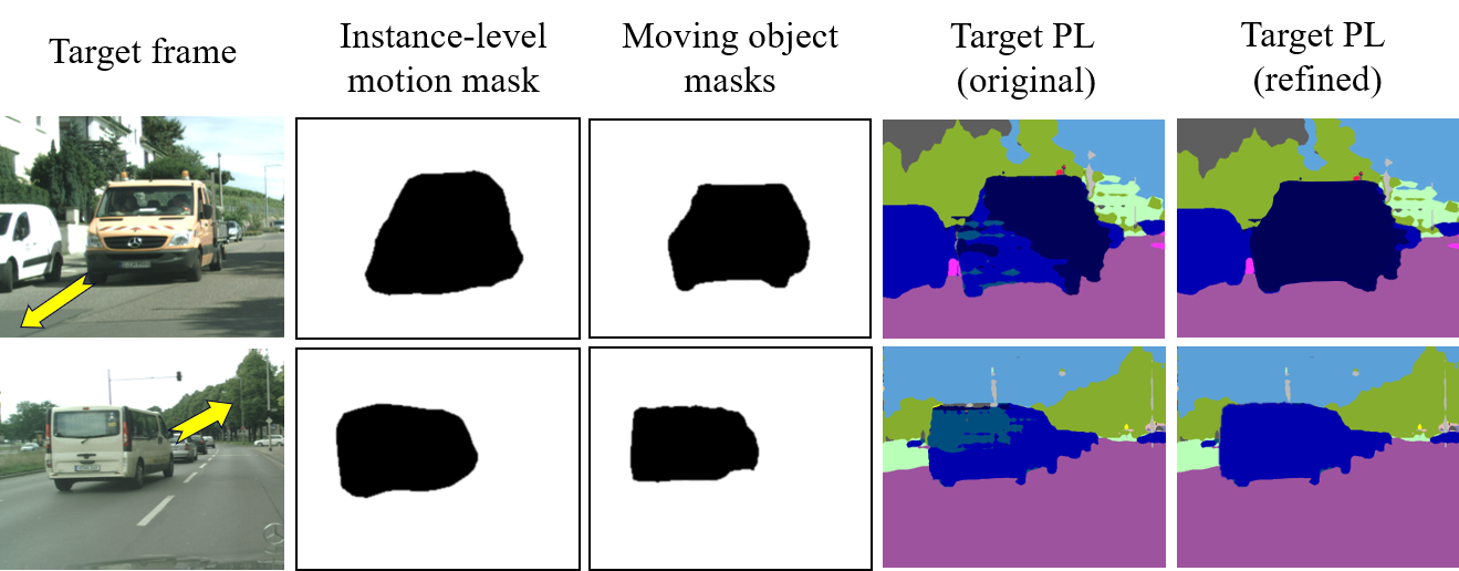
Figure 5: An illustration of foreground semantic mining (FSM) that takes the moving object masks as guidance to refine the target predictions on the foreground categories.

To align the domain gaps, we want to utilize the moving object masks generated by foreground object discovery (in Sec. IV-C) to improve the quality of the target pseudo labels. Specifically, we propose a foreground semantic mining (FSM) that takes the moving object masks as guidance to refine the noisy target predictions on the foreground categories. Our FSM is based on the assumption of rigidity of the moving objects, e.g., vehicles, and motorbikes on traffic roads. For example, if a vehicle is moving, all parts of the vehicle are moving together. Based on the rigidity of the moving objects, all the pixels covered by a moving object mask in an image must have the same categorical label. Subsequently, we have the following remark:

Remark 1. If a moving object mask is present, then the image pixels that it covers should have a semantic label that corresponds to the same moving categorical label.

Given a target pseudo label $\tilde{y}^{{}^{\prime}\mathbb{T}}$, we choose a dominant category $c^{*}$ in $\tilde{y}^{{}^{\prime}\mathbb{T}}$ that are covered by the moving object mask $o^{j}$. Concretely, $c^{*}$ is determined by the moving category with the highest occurrence. Based on Remark 1, we introduce a semantic mining weight $w\in\mathbb{R}^{H,W,C}$ to update the target pseudo label via

$$w_{(i,c)}=\lambda o^{j}_{(i)}\mathbbm{1}(c=c^{*}),$$ (17)

where $\mathbbm{1}(\cdot)$ is the indicator function, $o^{j}_{(i)}$ is the object mask value on the pixel $x_{(i)}^{\mathbb{T}}$, and $\lambda$ is a non-negative hyperparameter for scaling. Then, we update the target pseudo label using the following equation

$$\tilde{y}^{{}^{\prime}\mathbb{T}}=\Gamma(\texttt{softmax}((w+1)\odot p^{\mathbb{T}})),$$ (18)

where $\tilde{y}^{{}^{\prime}\mathbb{T}}$ is the updated target pseudo label by our target semantic mining, and $\Gamma$ is the process of taking the most probable category from $p^{\mathbb{T}}$ similar to Eq. 13. We provide an illustration of using object motion masks to update noisy target pseudo labels shown in Fig. 5. We use the updated target pseudo label to update the segmentation network $G_{e}$ by $\mathcal{L}_{FSM}$ which is defined by

$$\mathcal{L}_{FSM}=\sum_{i=1}^{H,W}\sum_{c=1}^{C}\tilde{y}_{(i,c)}^{{}^{\prime}\mathbb{T}}\log\big{(}G_{e}(x^{\mathbb{T}})\big{)}.$$ (19)

IV-E Cross-domain Background Adversarial Training (BAT)

We introduce a novel background domain alignment (BAT) method to align cross-domain background categories. We draw inspiration from the existing adversarial domain adaptation method [11] which aligns the domain gaps using the scene structure similarity between the source and target domain. However, our BAT differs in that we solely focus on aligning the background categories. Our assumption is that the scene structure of the source and the target domain mostly consist of background categories, e.g., the sky is usually at the top, the road is usually at the bottom, the buildings and the trees are usually at the side of the traffic road scene. This shows superior performance to [11] because the background categories in the source and target images share more structure similarity. The proposed BAT contains a background category-specific discriminator $D$. The background adversarial training loss $\mathcal{L}_{BAT}$ is defined by

$$\begin{split}\mathcal{L}_{BAT}=-\sum_{h,w}\log\big{(}1-D([G_{e}(x^{\mathbb{S}})]_{bg})_{(h,w,0)}\big{)}&\\ +\log\big{(}D([G_{e}(x^{\mathbb{T}})]_{bg})_{(h,w,1)}\big{)}&,\end{split}$$ (20)

where $[G_{e}(\cdot)]_{bg}$ is to take the predictions over the background categories from the segmentation network $G_{e}$. Since target data doesn’t have ground truth, we use the target pseudo labels to select background category predictions.

IV-F Overall Framework

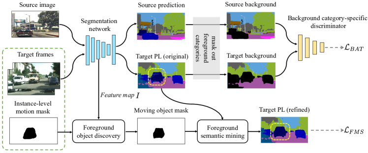
Figure 6: The overall framework of our motion-guided domain adaptation (MoDA) for semantic segmentation. MoDA proposes foreground object discovery (FOD) and foreground semantic mining (FSM) for cross-domain alignment on the foreground categories. Moreover, MoDA adopts background adversarial training (BAT) which contains a background category-specific discriminator for alignment on the background categories.

The proposed MoDA consists of three modules including motion mask preprocessing, self-supervised object discovery, and target semantic mining. We provide an overview of MoDA in Fig 6. Our overall objective function $\mathcal{L}_{MoDA}$ for training the segmentation network $G_{e}$ is composed of

$$\mathcal{L}_{MoDA}=\mathcal{L}_{FSM}+\mathcal{L}_{BAT}.$$ (21)

The final loss function $\mathcal{L}$ to optimize the segmentation network $G_{e}$ is represented by

$$\mathcal{L}=\mathcal{L}_{ce}^{\mathbb{S}}+\mathcal{L}_{ce}^{\mathbb{T}}+\mathcal{L}_{MoDA}.$$ (22)

IV-F1 Combine with temporal consistency regularization

One additional baseline is to use the temporal consistency across the adjacent target frames. Specifically, we can propagate the prediction of the previous frame to the current frame using optical flow estimates between the frames and subsequently ensure the consistency between the prediction of the current frame and the propagated prediction from the previous frame. Given two adjacent frames $\{x^{\mathbb{T}}_{1},x^{\mathbb{T}}_{2}\}$, we forward them as input to get the predictions $\{p^{\mathbb{T}}_{1},p^{\mathbb{T}}_{2}\}$. Moreover, we use FlowNet [43] to estimate the optical flow $f^{\mathbb{T}}_{1\to 2}$ from $x^{\mathbb{T}}_{1}$ to $x^{\mathbb{T}}_{2}$. Then we warp the prediction $p^{\mathbb{T}}_{1}$ to the propagated prediction $\bar{p}^{\mathbb{T}}_{2}$. Then the optical flow regularization loss $\mathcal{L}_{OFR}$ is formulated as

$$\mathcal{L}_{OFR}=\|p^{\mathbb{T}}_{1}-\bar{p}^{\mathbb{T}}_{2}\|_{2}.$$ (23)

We conduct an additional baseline method using temporal consistency regularization $\mathcal{L}_{TCR}$ that considers the temporal consistency of the target frames which is shown in Table VII.

V Experiment

In this work, We first describe the datasets and implementation details in Sec. V-A. Next, we report detailed domain adaption results for semantic segmentation and perform ablation studies to illustrate the effectiveness of our method. We evaluate the proposed MoDA on the domain adaptive image segmentation task in Sec. V-B1 and on the domain adaptive video segmentation task in Sec. V-B2. The ablation study and hyperparameter analysis are presented in Sec. V-C.

V-A Experiment Setup

V-A1 Datasets

For the task of domain adaptive image segmentation, we have GTA5 [4] and SYNTHIA [5] as the source domains. GTA5 contains 24,966 training images with the resolution $2,048\times 1,024$ and $19$ categories. SYNTHIA consists of 9,400 images with the resolution $1,280\times 760$, and $16$ categories. For the target domain, we use the 2,975 images and their adjacent frames collected from the videos in the Cityscapes dataset [3]. Thus, our newly created target dataset contains 5,950 training images and is named Cityscapes-AF. We also include 500 validation images from the Cityscapes dataset [3] for evaluation. For the task of domain adaptive video segmentation, we adopt VIPER [44] as the source domain and Cityscapes-AF as the target domain. VIPER [44] contains $133,670$ synthetic frames with the corresponding pixel-wise annotations from $77$ videos generated from game engines.

V-A2 Implementation details

We conduct experiments on two types of architectures: CNN-based architecture and Transformer-based architecture. For CNN-based architectures, we follow the setting in [9]. We first adopt DeepLab-V2 [2] with ReseNet-101 [45] for the segmentation network, pre-trained on ImageNet [46]. For Transformer-based architecture, we adopt MiT-B5 [47] as the encoder and incorporate our MoDA with existing state-of-the-art approaches [13, 6] by using the pre-trained weights from them. We train the network on the source data with ABN [48] and the target data with the self-training loss (Eq. 12), the foreground semantic mining loss (Eq. 19) and the background adversarial training loss (Eq. 20). Our batch size is 16 with 8 source and 8 target images with the resolution $1,024\times 512$. We adopt color jitter, random blur, and greyscaling for data augmentation (without random crop and fusion). Threshold $\tau$ is set with $0.5$. The optimizer for segmentation is SGD [49] with learning rate of $2.5e^{-4}$, momentum $0.9$, and weight decay of $5\times 10^{-4}$. We optimize the discriminator using Adam with the initial learning rate of $10^{-4}$. For the momentum network, we set $\lambda=0.99$. We implement MoDA with PyTorch and the training process is running on two Titan RTX A6000 GPUs.

TABLE I: The Comparison with state-of-the-art domain adaptive image segmentation approaches on GTA5$\to$Cityscapes-AF.

GTA5 $\to$ Cityscapes-AF
Method	Road	Side.	Buil.	Wall	Fence	Pole	TL	TS	Vege.	Terr.	Sky	Pers.	Rider	Car	Truck	Bus	Train	Motor	Bike	mIoU
Backbone: ResNet-101
Baseline [9]	91.2	53.7	83.0	31.9	25.6	24.9	28.3	26.4	82.9	36.2	82.9	52.1	25.5	81.5	29.1	36.1	14.9	24.8	42.8	46.0
MoDA-fg	91.6	50.3	79.8	31.2	22.7	24.8	28.5	23.1	81.3	35.8	81.1	58.2	29.2	88.2	47.5	50.0	22.6	33.0	54.1	49.1
MoDA-bg	93.1	56.4	83.3	33.8	27.2	25.9	33.1	26.9	85.6	38.9	82.9	52.4	27.9	81.7	30.6	36.1	15.0	23.7	43.0	47.2
MoDA	93.3	56.5	83.8	33.0	27.7	25.8	33.7	26.2	85.7	38.3	83.5	58.7	29.3	88.0	48.0	50.1	22.7	33.3	51.9	51.0
AdatpSegNet [11]	86.3	36.2	79.8	24.1	23.9	24.1	36	15.2	82.6	31.9	74.4	58.7	26.8	75.1	33.9	35.8	4.1	29.7	28.8	42.5
AdvEnt [10]	91.6	54	79.8	32.4	21.5	33.6	29.1	21.7	84.2	35.4	81.7	52.9	23.8	81.9	31	35.3	16.8	26.2	43.7	46.1
IntraDA [21]	91.6	38.1	81.7	33	20.4	28.6	31.9	22.7	85.6	41.1	78.9	59.2	31.8	86.1	31.9	48.3	0.2	30.9	35.7	46.2
CRST [24]	90.0	56.1	83.3	32.8	24.5	36.6	33.7	25.4	84.9	35.3	81.0	58.3	25.6	84	28.7	31.8	27.4	25.8	42.9	47.8
SIM [50]	89.8	46.1	85.9	33.5	27.8	36.7	35	37.6	84.7	45.4	83.2	56.4	31.5	82.7	43.2	49.9	2.1	33.4	38.7	49.7
CAG-UDA [51]	90.4	51.6	83.8	34.2	27.8	38.4	25.3	48.4	85.4	38.2	78.1	58.6	34.6	84.7	21.9	42.7	41.1	29.3	37.2	50.2
IAST [52]	93.8	57.8	85.1	39.5	26.7	26.2	43.1	34.7	84.9	32.9	88.0	62.6	29.0	87.3	39.2	49.6	23.2	34.7	39.6	51.5
DACS [26]	90.4	40.1	86.6	31.4	40.8	39.2	45.8	53.4	88.6	42.7	89.5	66.1	35.7	85.6	46.7	51.3	0.2	28.7	34.6	52.5
ProDA [7]	86.5	57.3	80.7	45.8	45.7	46.4	53.6	54.2	88.6	46.1	81.8	70.9	40.3	89.1	44.7	60.4	1.4	49.5	57.4	57.9
+MoDA	86.9	57.5	81.9	46.2	45.4	46.6	54.3	52.5	88.9	48.4	81.4	70.6	43.5	90.3	90.3	60.3	8.2	50.4	61.3	61.3
SePiCo [14]	96.5	70.1	88.4	41.5	37.7	44.1	55.9	65.5	88.9	46.1	89.2	74.9	56.1	90.8	59.3	54.2	6.1	23.3	44.4	59.6
+MoDA	97.2	70.0	88.5	41.9	40.2	45.2	57.3	64.6	89.1	45.9	89.4	75.2	56.2	91.3	63.5	66.4	12.1	34.7	50.1	62.0
Backbone: Transformer
DAFormer [13]	95.3	69.9	89.7	52.8	48.4	49.7	55.3	60.4	91.0	48.2	92.6	72.1	44.9	93.4	74.7	78.2	64.8	56.3	60.9	68.3
+MoDA	95.7	70.4	90.4	52.1	49.8	50.0	56.7	60.8	91.8	46.8	93.3	75.1	49.5	93.2	76.7	82.1	65.2	64.8	67.5	73.4
HRDA [6]	97.1	74.5	90.8	62.2	51.0	58.2	63.4	70.5	92.0	48.3	94.6	78.8	53.1	94.5	83.6	84.9	76.8	64.3	65.7	73.9
+MoDA	97.3	74.5	91.4	61.4	51.4	59.2	64.1	70.0	91.0	49.5	95.9	80.1	57.1	95.1	83.1	89.4	77.5	72.0	68.8	75.2

V-B Evaluation Results

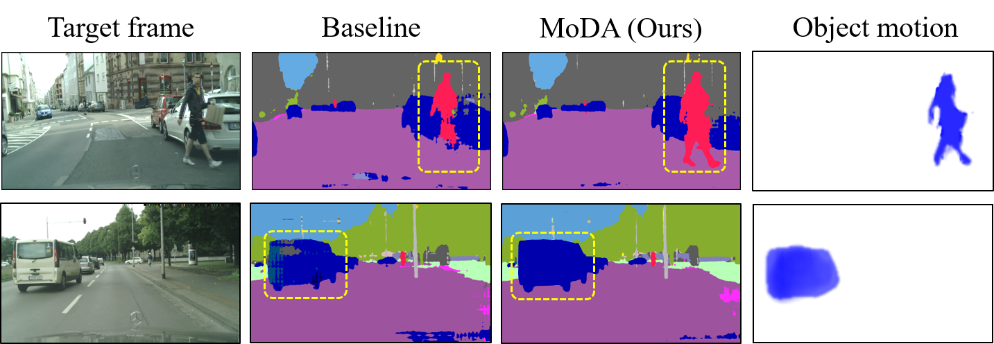
Figure 7: Qualitative results of MoDA utilizing the object motion as guidance for domain adaptation.

V-B1 Comparison with the state-of-the-art unsupervised domain adaption approaches

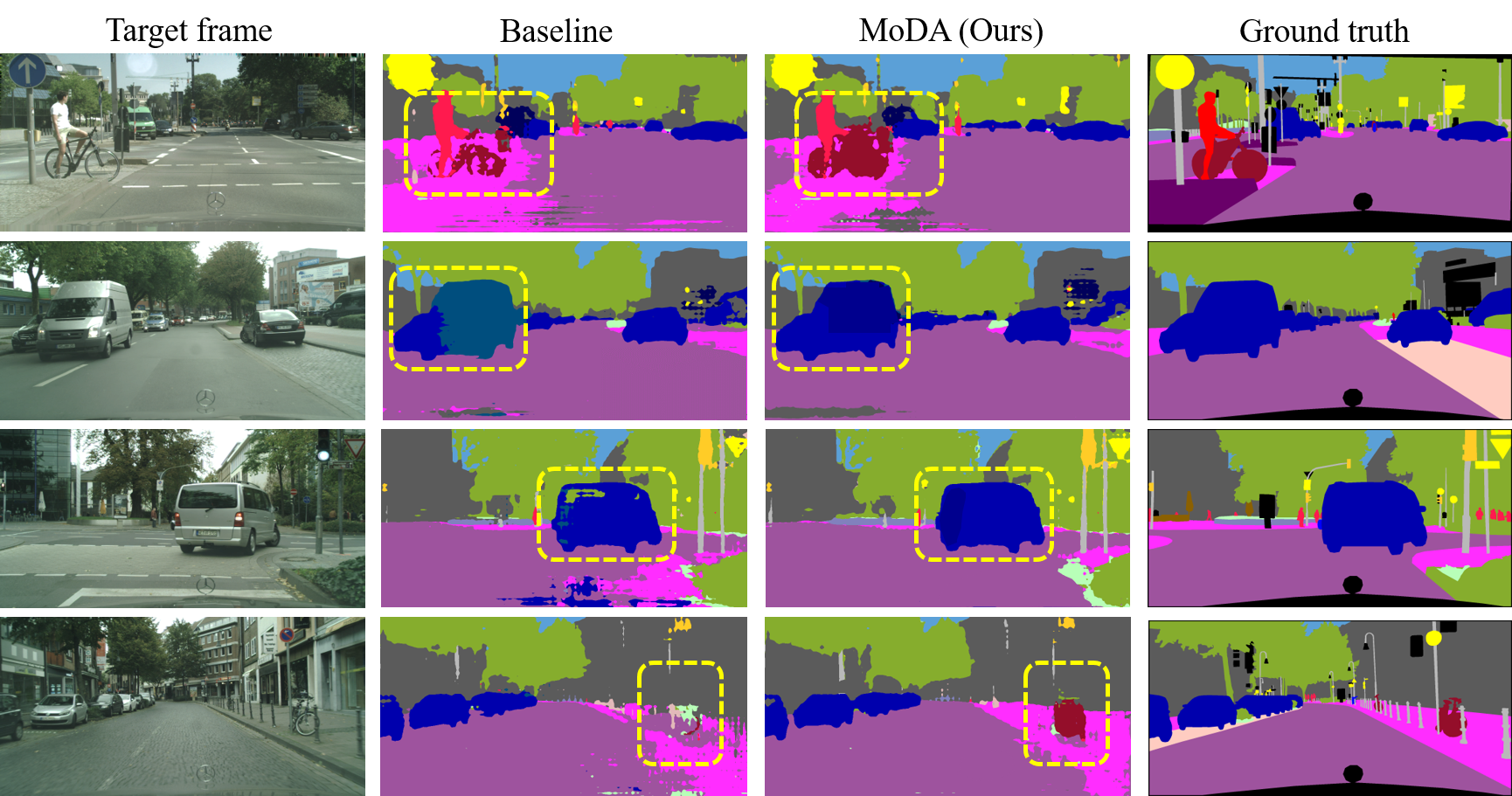
Figure 8: Comparison of the qualitative results generated from MoDA and the baseline model on GTA5$\to$Cityscapes-AF benchmark.

We evaluate the performance of MoDA in Table I and Table II. To make a fair comparison, all the unsupervised domain adaptation baselines are trained with GTA5/SYNTHIA as the source and Cityscapes-AF as the target domain. For CNN-based architecture, our baseline model contains a segmentation network and a momentum network with ResNet101-based [45] DeepLab-v2 [2] architecture. To ensure a fair comparison, the baseline model is a vanilla self-training following [9]. The baseline is trained with source data using ABN [48] and with target data using data augmentation including color jittering, random blur, and random flipping. We also analyze MoDA’s efficacy on the alignment of the foreground and background categories, respectively. The results of MoDA-fg are generated by aligning foreground categories only, using FOD & FSM while removing BAT. The results of MoDA-bg are obtained by aligning background categories using BAT solely, with FOD & FSM removed. Moreover, we provide qualitative results of MoDA in Fig. 7 and Fig. 8. Additionally, we demonstrate that MoDA complements existing UDA approaches by incorporating MoDA for the performance boost, denoted as +MoDA. The results of +MoDA are obtained by the model trained with the target pseudo labels generated from existing approaches.

We include existing ResNet-101 based approaches for comparison: AdaptSegNet [11], AdvEnt [10], IntraDA [21], SIM [50], CRST [24], CAG-UDA [51], IAST [52], DACS [26], ProDA [7], and SePiCo [14]. Additionally, we experiment with MoDA on two transformer-based UDA approaches, DAFormer [13] and HRDA [6]. Note that all the approaches above are trained with GTA5/SYNTHIA as the source and Cityscapes-AF as the target domain to make a fair evaluation.

GTA5$\rightarrow$Cityscapes-AF. Table I presents comparison results on the adaptation from GTA5 $\to$ Cityscapes-AF. Our MoDA, MoDA-fg, and MoDA-bg achieve $51.0\%$, $49.1\%$, and $47.2\%$ of mIoU across the total 19 categories, respectively, which are all higher than the baseline, demonstrating the effectiveness of our proposed three modules FOD, FSM, and BAT. MoDA-fg outperforms the baseline by $3.2\%$ of mIoU. Notably, in the detailed category-level comparison, MoDA-fg considerably improves the baseline in terms of the foreground categories, such as motorcycle, bike, train, bus, truck, etc. The improvement in the foreground categories is attributed to the use of the proposed FOD & FSM for domain alignment. Similarly, the score of MoDA-bg reaches $47.2\%$, outperforming the baseline by $1.2\%$, where the performance increases noticeably on background categories like road, sidewalk, wall, and traffic light. This demonstrates the efficacy of BAT in bridging the gaps of the background categories. +MoDA provides consistent performance improvement on ProDA [7] from $57.9\%$ to $61.3\%$, SePiCo [14] from $59.6\%$ to $62.0\%$, DAFormer [13] from $68.3\%$ to $73.4\%$, and HRDA [6] from $73.9\%$ to $75.2\%$. It shows the versatility of MoDA to be combined with state-of-the-art approaches with both CNN-based and transformer-based architecture.

TABLE II: The comparison results with state-of-the-art domain adaptive image segmentation approaches on SYNTHIA$\to$Cityscapes-AF. Note that $\text{mIoU}^{13}$ is generated among the 13 categories without wall, fence, and pole.

SYNTHIA $\to$ Cityscapes-AF
Method	Road	Side.	Buil.	$\text{Wall}^{*}$	$\text{Fence}^{*}$	$\text{Pole}^{*}$	TL	TS	Vege.	Sky	Pers.	Rider	Car	Bus	Motor	Bike	mIoU	$\text{mIoU}^{13}$
Backbone: ResNet-101
Baseline [9]	68.2	29.7	76.4	11.0	1.6	33.7	22.9	30.1	78.3	77.9	60.8	28.2	81.5	23.1	18.9	39.7	42.6	48.9
MoDA-fg	69.7	28.3	76.6	10.4	1.7	34.8	23.8	27.2	78.5	78.2	71.7	33.4	88.5	34.6	26.1	46.4	45.6	52.5
MoDA-bg	70.8	31.7	77.6	10.3	2.8	35.8	27.5	31.8	79.3	81.8	60.1	26.1	81.8	22.0	17.2	39.2	43.5	49.8
MoDA	71.1	31.8	77.9	11.8	2.7	36.0	27.3	33.9	80.4	82.0	70.9	34.2	88.4	35.0	27.2	45.7	47.2	54.3
AdaptSeg [11]	79.5	37.1	79.3	10.8	0.5	24.9	9.4	11.3	78.8	80.8	54.1	19.7	67.4	29.7	21.5	32.0	39.8	52.9
AdvEnt [10]	86.1	42.3	79.8	8.1	0.5	26.6	5.3	8.9	81.4	84.5	58.3	24.7	73.6	36.2	14.3	33.3	41.5	55.7
IntraDA [21]	85.6	38.1	79.9	5.2	0.3	24.8	9.4	8.5	80.2	84.4	57.3	23.6	77.9	38.2	20.5	36.7	41.9	55.8
CRST [24]	68.4	33.1	73.4	10.5	1.7	37.2	22.3	31.1	80.9	81.5	61.2	27.9	82.4	25.5	19.8	45.7	43.9	50.4
CAG-UDA [51]	84.7	40.8	81.7	7.8	0.0	35.1	13.3	22.7	84.5	77.6	64.2	27.8	80.9	19.7	22.7	48.3	44.5	51.4
IAST [52]	81.9	41.5	83.3	17.7	4.6	32.3	30.9	28.8	83.4	85.0	65.5	30.8	86.5	38.2	33.1	52.7	49.8	57.0
DACS [26]	80.7	25.2	82.5	21.6	3.3	37.4	22.8	24.3	83.6	90.7	67.9	39.4	83.2	39.4	28.6	47.7	48.6	57.8
ProDA [7]	87.5	45.6	84.7	37.5	0.8	44.1	54.8	36.9	88.0	84.2	74.3	24.5	88.1	51.4	40.6	45.9	55.6	62.1
+MoDA	87.6	45.8	85.5	37.6	1.1	43.8	55.3	36.5	88.2	85.8	75.9	27.6	91.2	62.6	49.1	54.2	57.9	65.0
SePiCo [14]	79.8	43.1	85.7	10.2	4.3	38.5	50.3	53.4	80.8	81.4	73.8	47.5	86.5	63.8	47.6	62.5	58.0	67.1
+MoDA	80.1	44.0	85.8	10.9	3.3	38.0	50.4	55.9	80.9	81.6	77.6	56.5	91.1	64.2	52.1	67.2	58.7	68.3
Backbone: Transformer
DAFormer [13]	85.0	40.6	88.3	41.6	6.4	49.8	54.7	54.3	86.7	89.9	73.5	48.7	88.0	52.9	54.1	61.5	61.0	68.9
+MoDA	85.4	41.4	88.7	41.2	7.1	50.2	56.8	55.7	86.8	90.4	75.0	54.7	90.6	58.9	54.3	63.3	62.5	69.4
HRDA [6]	85.5	47.2	88.6	49.7	4.3	57.1	65.9	60.5	85.5	93.1	79.8	52.7	88.9	64.4	63.8	65.2	65.8	72.9
+MoDA	86.2	47.5	89.7	49.3	4.5	57.9	65.2	60.9	86.7	93.8	80.2	55.4	92.3	64.0	64.3	68.7	66.6	73.4

SYNTHIA$\rightarrow$Cityscapes-AF. In Table II, we compare domain adaptation results from SYNTHIA to Cityscapes-AF. In both the 16 and the 13 categories’ settings, the results from MoDA, MoDA-fg, and MoDA-bg achieve higher mIoU scores than the baseline. Under the 16 and 13 category settings, the mIoU scores of MoDA reach to $46.9\%$ and $55.7\%$, which are $4.3\%$ and $3.6\%$ higher than the baseline. On the foreground alignment, MoDA-fg achieves $45.6\%$ and $52.5\%$ which are $3.0\%$ and $3.5\%$ higher than the baseline under the 16 and 13 category settings. MoDA-bg reaches to $43.5\%$ and $49.8\%$, outperforming the baseline by $0.9\%$ and $0.9\%$ in the 16 and 13 category setting. Additionally, the use of +MoDA consistently improve the performance of state-of-the-art approaches ProDA [7], SePiCo [14], DAFormer [13], and HRDA [6].

V-B2 Comparison with the state-of-the-art domain adaptive video segmentation approaches

TABLE III: The comparison results with state-of-the-art domain adaptive video segmentation approaches on VIPER$\to$Cityscapes-AF.

VIPER $\to$ Cityscapes-AF
Method	Road	Side.	Buil.	Fence	TL	TS	Vege.	Terr.	Sky	Pers.	Car	Truck	Bus	Motor	Bike	mIoU
PixMatch [53]	78.5	27.1	83.9	16.4	29.1	23.3	84.5	30.2	83.9	58.4	75.3	34.6	44.5	17.2	13.1	46.6
DA-VSN [37]	87.1	36.3	84.2	23.7	29.8	28.4	85.9	26.6	80.8	60.3	78.7	21.7	46.9	22.0	10.5	48.2
TPS [15]	83.4	35.8	78.9	9.6	25.7	29.5	77.9	28.4	81.6	60.2	81.1	40.7	39.8	27.7	31.4	48.7
MoDA	88.7	37.4	86.7	14.3	26.6	30.4	79.1	27.2	84.3	70.7	84.1	43.2	47.5	28.3	40.6	52.6

We evaluate MoDA in the setting of domain adaptive video segmentation: VIPER$\to$Cityscapes-AF. We choose state-of-the-art domain adaptive video segmentation approaches PixMatch [53], DA-VSN [37], and TPS [15] as our baseline models. The experimental results are shown in Table III. According to Table III, MoDA outperforms TPS [15] by $3.9\%$ mIoU, which shows the superiority of MoDA using object motion over existing domain adaptive video segmentation approaches.

V-C Ablation Study

V-C1 Ablation study on the components of MoDA

TABLE IV: Ablation study on the components of MoDA.

Configuration	FOD	FSM	BAT	mIoU	Gap
w/o Background Adversarial Training	✓	✓		49.1	-1.9
w/o Foreground Semantic Mining			✓	47.2	-3.8
w/o Foreground Object Discovery		✓	✓	49.4	-1.6
Full Framework (MoDA)	✓	✓	✓	51.0	-

We conduct an ablation study on the effectiveness of foreground object discovery (FOD), foreground semantic mining (FSM), and background adversarial training (BAT) in Table IV. Based on evaluation on GTA5$\to$Cityscapes-AF, by only using FOD & FSM (without using BAT), the performance drops to $49.1\%$ of mIoU. On the other hand, only utilizing BAT (without using FOD & FSM), MoDA experienced a more significant decline to $47.2\%$ of mIoU. Moreover, using FSM & BAT (without using FOD) the performance drops to $49.6\%$ of mIoU. Combining all three modules FOD, FSM, and BAT, MoDA achieves $51.0\%$ of mIoU.

V-C2 Unreliable motion masks

We evaluate the effects of the unreliable motion mask from the motion network for MoDA. MoDA consists of foreground object discovery (FOD) which is to find the accurate moving object masks with a self-supervised attention mechanism. According to Table IV, by using FSM & BAT (without using FOD) the performance reaches $49.6\%$ of mIoU. Adding FOD to the framework, the mIoU score increases to $51.0\%$ mIoU. It shows the important role of FOD in handling unreliable motion masks from the motion network.

V-C3 Background adversarial training

TABLE V: Background adversarial training.

Method	mIoU (bg categories)	Gain
Existing Adversarial Training [11]	50.7	-
Background Adversarial Training	53.4	+2.7

We compare background adversarial training (BAT) with the standard adversarial training [11]. We present an ablation study on the mIoU performance of the background categories on GTA5$\to$Cityscapes-AF. Our BAT alignment achieves $53.4\%$ with a gain of $2.7\%$, in comparison with the standard adversarial training. These results suggest that separating the foreground and background categories in BAT leads to better alignment on the background categories.

V-C4 Hyperparameter $\lambda$

TABLE VI: The analysis on the hyperparameter $\lambda$ for scaling in foreground semantic mining.

$\lambda$	0.0	0.2	0.4	0.6	0.8	1.0	1.2	1.4
mIoU	47.2	48.7	49.9	50.7	51.0	50.9	51.0	51.0

We conduct an ablation study on the hyperparameter $\lambda$ in foreground semantic mining (Eq. 17). We present different values of $\lambda$ for the final performance in GTA5$\to$Cityscapes-AF in Table VI. The bigger value of $\lambda$ put more weight on foreground semantic mining on target pseudo label updating. Our ablation results indicate that MoDA reaches the best performance when $\lambda$ reaches $0.8$. Additionally, the results suggest that the mIoU performance of MoDA is not significantly affected by the value of the hyperparameter $\lambda$ when it is greater than $0.8$.

V-C5 Temporal consistency regularization

TABLE VII: Comparison with Temporal consistency regularization (TCR).

Configuration	$\mathcal{L}_{ce}^{\mathbb{S}}$	$\mathcal{L}_{ce}^{\mathbb{T}}$	$\mathcal{L}_{MoDA}$	$\mathcal{L}_{TCR}$	mIoU	Gain
Baseline [9]	✓	✓			46.0	-
TCR	✓	✓		✓	47.4	+1.4
MoDA	✓	✓	✓		51.0	+5.0
MoDA+TCR	✓	✓	✓	✓	52.3	+6.3

We provide quantitative analysis on using object motion as guidance in comparison with the temporal consistency regularization (in Sec IV-F1). We show the evaluation of GTA5$\to$Cityscapes-AF in Table VII. We achieve $47.4\%$ of mIoU by using temporal consistency regularization (TCR) which is $1.4\%$ higher than the baseline model [9]. By using MoDA we produce $51.0\%$ of mIoU which are much higher than using TCR. This shows the superiority of MoDA as guidance for domain alignment. We further combine MoDA with TCR to further boost the performance up to $52.2\%$ of mIoU.

V-C6 What happens to the potentially movable, but static objects (e.g., parked cars, standing persons)

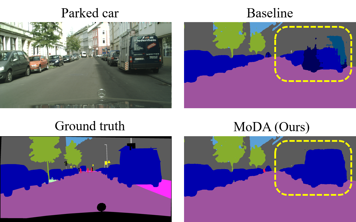
Figure 9: The proposed MoDA can learn effective representations for the parked objects.

First of all, the overall training pipeline of our approach does not harm static objects like parked cars or standing pedestrians during the domain transfer. Since MoDA uses motion-guided object masks to update the noisy predictions of the pseudo labels, the performance on static objects will also be upgraded by updating the segmentation net with these new pseudo labels. As an example in Fig. 9, MoDA generates more accurate predictions on the parked vehicle which is not moving in comparison with the baseline [9].

VI Conclusion

This paper proposed a novel motion-guide domain adaption method, namely MoDA for the semantic segmentation task. MoDA addresses the domain alignment separately for the foreground and background categories using different strategies. For foreground categories, MoDA employs foreground object discovery (FOD) and foreground semantic mining (FSM), using motion as guidance at the object level. For background alignment, MoDA introduces background adversarial training (BAT) that includes a background category-specific discriminator. Our experiments on various benchmarks demonstrate MoDA’s effectiveness compared to existing approaches. Furthermore, MoDA is adaptable and can be used alongside state-of-the-art methods to further enhance performance.

References

- [1] J. Long, E. Shelhamer, and T. Darrell, “Fully convolutional networks for semantic segmentation,” in IEEE Conf. Comput. Vis. Pattern Recog., Boston, US, 2015, pp. 3431–3440.
- [2] L.-C. Chen, G. Papandreou, I. Kokkinos, K. Murphy, and A. L. Yuille, “Deeplab: Semantic image segmentation with deep convolutional nets, atrous convolution, and fully connected crfs,” IEEE Trans. Pattern Anal. Mach. Intell., vol. 40, no. 4, pp. 834–848, 2017.
- [3] M. Cordts, M. Omran, S. Ramos, T. Rehfeld, M. Enzweiler, R. Benenson, U. Franke, S. Roth, and B. Schiele, “The cityscapes dataset for semantic urban scene understanding,” in IEEE Conf. Comput. Vis. Pattern Recog., Las Vegas, Nevada, 2016, pp. 3213–3223.
- [4] S. R. Richter, V. Vineet, S. Roth, and V. Koltun, “Playing for data: Ground truth from computer games,” in Eur. Conf. Comput. Vis. Amsterdam, US: Springer, 2016, pp. 102–118.
- [5] G. Ros, L. Sellart, J. Materzynska, D. Vazquez, and A. M. Lopez, “The synthia dataset: A large collection of synthetic images for semantic segmentation of urban scenes,” in IEEE Conf. Comput. Vis. Pattern Recog., Las Vegas, Nevada, 2016, pp. 3234–3243.
- [6] L. Hoyer, D. Dai, and L. Van Gool, “Hrda: Context-aware high-resolution domain-adaptive semantic segmentation,” in Eur. Conf. Comput. Vis. Tel Aviv, Israel: Springer, 2022, pp. 372–391.
- [7] P. Zhang, B. Zhang, T. Zhang, D. Chen, Y. Wang, and F. Wen, “Prototypical pseudo label denoising and target structure learning for domain adaptive semantic segmentation,” in IEEE Conf. Comput. Vis. Pattern Recog., Virtual/Online, 2021, pp. 12 414–12 424.
- [8] Y. Cao, H. Zhang, X. Lu, Y. Chen, Z. Xiao, and Y. Wang, “Adaptive refining-aggregation-separation framework for unsupervised domain adaptation semantic segmentation,” IEEE Trans. Circuit Syst. Video Technol., 2023.
- [9] N. Araslanov and S. Roth, “Self-supervised augmentation consistency for adapting semantic segmentation,” in IEEE Conf. Comput. Vis. Pattern Recog., Virtual/Online, 2021, pp. 15 384–15 394.
- [10] T.-H. Vu, H. Jain, M. Bucher, M. Cord, and P. Pérez, “Advent: Adversarial entropy minimization for domain adaptation in semantic segmentation,” in IEEE Conf. Comput. Vis. Pattern Recog., Long Beach, US, 2019, pp. 2517–2526.
- [11] Y.-H. Tsai, W.-C. Hung, S. Schulter, K. Sohn, M.-H. Yang, and M. Chandraker, “Learning to adapt structured output space for semantic segmentation,” in IEEE Conf. Comput. Vis. Pattern Recog., Salt Lake City, US, 2018, pp. 7472–7481.
- [12] H. Tian, S. Qu, and P. Payeur, “A prototypical knowledge oriented adaptation framework for semantic segmentation,” IEEE Trans. Image Process., vol. 31, pp. 149–163, 2022.
- [13] L. Hoyer, D. Dai, and L. Van Gool, “Daformer: Improving network architectures and training strategies for domain-adaptive semantic segmentation,” in IEEE Conf. Comput. Vis. Pattern Recog., New Orleans, US, 2022, pp. 9924–9935.
- [14] B. Xie, S. Li, M. Li, C. H. Liu, G. Huang, and G. Wang, “Sepico: Semantic-guided pixel contrast for domain adaptive semantic segmentation,” IEEE Trans. Pattern Anal. Mach. Intell., 2023.
- [15] Y. Xing, D. Guan, J. Huang, and S. Lu, “Domain adaptive video segmentation via temporal pseudo supervision,” in Eur. Conf. Comput. Vis. Tel Aviv, Israel: Springer, 2022, pp. 621–639.
- [16] H. Li, A. Gordon, H. Zhao, V. Casser, and A. Angelova, “Unsupervised monocular depth learning in dynamic scenes,” in Conf. on Robot Learn. London, UK: PMLR, 2021, pp. 1908–1917.
- [17] S. Lee, F. Rameau, F. Pan, and I. S. Kweon, “Attentive and contrastive learning for joint depth and motion field estimation,” in Int. Conf. Comput. Vis., Virtual/Online, 2021, pp. 4862–4871.
- [18] A. Gordon, H. Li, R. Jonschkowski, and A. Angelova, “Depth from videos in the wild: Unsupervised monocular depth learning from unknown cameras,” in Int. Conf. Comput. Vis., Seoul, South Korea, 2019, pp. 8977–8986.
- [19] M. Toldo, A. Maracani, U. Michieli, and P. Zanuttigh, “Unsupervised domain adaptation in semantic segmentation: a review,” Technologies, vol. 8, no. 2, p. 35, 2020.
- [20] G. Csurka, R. Volpi, and B. Chidlovskii, “Unsupervised domain adaptation for semantic image segmentation: a comprehensive survey,” 2021. [Online]. Available: https://arxiv.org/abs/2112.03241
- [21] F. Pan, I. Shin, F. Rameau, S. Lee, and I. S. Kweon, “Unsupervised intra-domain adaptation for semantic segmentation through self-supervision,” in IEEE Conf. Comput. Vis. Pattern Recog., Seattle, US, 2020, pp. 3764–3773.
- [22] R. Li, W. Cao, S. Wu, and H.-S. Wong, “Generating target image-label pairs for unsupervised domain adaptation,” IEEE Trans. Image Process., vol. 29, pp. 7997–8011, 2020.
- [23] Q. Wang, J. Gao, and X. Li, “Weakly supervised adversarial domain adaptation for semantic segmentation in urban scenes,” IEEE Trans. Image Process., vol. 28, no. 9, pp. 4376–4386, 2019.
- [24] Y. Zou, Z. Yu, X. Liu, B. Kumar, and J. Wang, “Confidence regularized self-training,” in Int. Conf. Comput. Vis., Seoul, South Korea, 2019, pp. 5982–5991.
- [25] Y. Zou, Z. Yu, B. Kumar, and J. Wang, “Unsupervised domain adaptation for semantic segmentation via class-balanced self-training,” in Eur. Conf. Comput. Vis., Munich, Germany, 2018, pp. 289–305.
- [26] W. Tranheden, V. Olsson, J. Pinto, and L. Svensson, “Dacs: Domain adaptation via cross-domain mixed sampling,” in Proc. of IEEE/CVF Wint. Conf. on Appli. of Comput. Visi., Hawaii, USA., 2021, pp. 1379–1389.
- [27] Z. Zheng and Y. Yang, “Rectifying pseudo label learning via uncertainty estimation for domain adaptive semantic segmentation,” Int. J. Comput. Vis., vol. 129, no. 4, pp. 1106–1120, 2021.
- [28] M. Kim and H. Byun, “Learning texture invariant representation for domain adaptation of semantic segmentation,” in IEEE Conf. Comput. Vis. Pattern Recog., Seattle, US, 2020, pp. 12 975–12 984.
- [29] Z. Lu, D. Li, Y.-Z. Song, T. Xiang, and T. M. Hospedales, “Uncertainty-aware source-free domain adaptive semantic segmentation,” IEEE Trans. Image Process., pp. 1–1, 2023.
- [30] Z. Zheng and Y. Yang, “Unsupervised scene adaptation with memory regularization in vivo,” 2019. [Online]. Available: https://arxiv.org/abs/1912.11164
- [31] S. Wang, D. Zhao, C. Zhang, Y. Guo, Q. Zang, Y. Gu, Y. Li, and L. Jiao, “Cluster alignment with target knowledge mining for unsupervised domain adaptation semantic segmentation,” IEEE Trans. Image Process., vol. 31, pp. 7403–7418, 2022.
- [32] B. Yuan, D. Zhao, S. Shao, Z. Yuan, and C. Wang, “Birds of a feather flock together: Category-divergence guidance for domain adaptive segmentation,” IEEE Trans. Image Process., vol. 31, pp. 2878–2892, 2022.
- [33] Y. Zhao, Z. Zhong, Z. Luo, G. H. Lee, and N. Sebe, “Source-free open compound domain adaptation in semantic segmentation,” IEEE Trans. Circuit Syst. Video Technol., vol. 32, no. 10, pp. 7019–7032, 2022.
- [34] V. Guizilini, J. Li, R. Ambruș, and A. Gaidon, “Geometric unsupervised domain adaptation for semantic segmentation,” in Int. Conf. Comput. Vis., Virtual/Online, 2021, pp. 8537–8547.
- [35] W. Zhou, Y. Wang, J. Chu, J. Yang, X. Bai, and Y. Xu, “Affinity space adaptation for semantic segmentation across domains,” IEEE Trans. Image Process., vol. 30, pp. 2549–2561, 2021.
- [36] J. Munro and D. Damen, “Multi-modal domain adaptation for fine-grained action recognition,” in IEEE Conf. Comput. Vis. Pattern Recog., Seattle, US, 2020, pp. 122–132.
- [37] D. Guan, J. Huang, A. Xiao, and S. Lu, “Domain adaptive video segmentation via temporal consistency regularization,” in Int. Conf. Comput. Vis., Virtual/Online, 2021, pp. 8053–8064.
- [38] Z. Cao, A. Kar, C. Hane, and J. Malik, “Learning independent object motion from unlabelled stereoscopic videos,” in IEEE Conf. Comput. Vis. Pattern Recog., 2019.
- [39] Z. Wang, A. C. Bovik, H. R. Sheikh, and E. P. Simoncelli, “Image quality assessment: from error visibility to structural similarity,” IEEE Trans. Image Process., 2004.
- [40] C. Godard, O. Mac Aodha, and G. J. Brostow, “Unsupervised monocular depth estimation with left-right consistency,” in IEEE Conf. Comput. Vis. Pattern Recog., Hawaii, US, 2017.
- [41] K. Wu, E. Otoo, and A. Shoshani, “Optimizing connected component labeling algorithms,” in Medic. Imagi.: Image Processing, vol. 5747. SPIE, 2005.
- [42] A. Tarvainen and H. Valpola, “Mean teachers are better role models: Weight-averaged consistency targets improve semi-supervised deep learning results,” Adv. Neural Inform. Process. Syst., vol. 30, 2017.
- [43] E. Ilg, N. Mayer, T. Saikia, M. Keuper, A. Dosovitskiy, and T. Brox, “Flownet 2.0: Evolution of optical flow estimation with deep networks,” in IEEE Conf. Comput. Vis. Pattern Recog., Hawaii, US, 2017, pp. 2462–2470.
- [44] S. R. Richter, Z. Hayder, and V. Koltun, “Playing for benchmarks,” in Int. Conf. Comput. Vis., 2017.
- [45] K. He, X. Zhang, S. Ren, and J. Sun, “Deep residual learning for image recognition,” in IEEE Conf. Comput. Vis. Pattern Recog., Las Vegas, Nevada, 2016, pp. 770–778.
- [46] J. Deng, W. Dong, R. Socher, L.-J. Li, K. Li, and L. Fei-Fei, “Imagenet: A large-scale hierarchical image database,” in IEEE Conf. Comput. Vis. Pattern Recog. Miami, USA: Ieee, 2009, pp. 248–255.
- [47] E. Xie, W. Wang, Z. Yu, A. Anandkumar, J. M. Alvarez, and P. Luo, “Segformer: Simple and efficient design for semantic segmentation with transformers,” Adv. Neural Inform. Process. Syst., vol. 34, pp. 12 077–12 090, 2021.
- [48] Y. Li, N. Wang, J. Shi, X. Hou, and J. Liu, “Adaptive batch normalization for practical domain adaptation,” Pattern Recognition, vol. 80, pp. 109–117, 2018.
- [49] L. Bottou, “Large-scale machine learning with stochastic gradient descent,” in Int. Conf. on Comput. Statis. Paris, France: Springer, 2010, pp. 177–186.
- [50] Z. Wang, M. Yu, Y. Wei, R. Feris, J. Xiong, W.-m. Hwu, T. S. Huang, and H. Shi, “Differential treatment for stuff and things: A simple unsupervised domain adaptation method for semantic segmentation,” in IEEE Conf. Comput. Vis. Pattern Recog., Seattle, US, 2020, pp. 12 635–12 644.
- [51] Q. Zhang, J. Zhang, W. Liu, and D. Tao, “Category anchor-guided unsupervised domain adaptation for semantic segmentation,” Adv. Neural Inform. Process. Syst., vol. 32, 2019.
- [52] K. Mei, C. Zhu, J. Zou, and S. Zhang, “Instance adaptive self-training for unsupervised domain adaptation,” in Eur. Conf. Comput. Vis. Glasgow, UK: Springer, 2020, pp. 415–430.
- [53] L. Melas-Kyriazi and A. K. Manrai, “Pixmatch: Unsupervised domain adaptation via pixelwise consistency training,” in IEEE Conf. Comput. Vis. Pattern Recog., Virtual/Online, 2021, pp. 12 435–12 445.