\ul
Dr. FERMI: A Stochastic Distributionally Robust Fair Empirical Risk Minimization Framework
Abstract
While training fair machine learning models has been studied extensively in recent years, most developed methods rely on the assumption that the training and test data have similar distributions. In the presence of distribution shifts, fair models may behave unfairly on test data. There have been some developments for fair learning robust to distribution shifts to address this shortcoming. However, most proposed solutions are based on the assumption of having access to the causal graph describing the interaction of different features. Moreover, existing algorithms require full access to data and cannot be used when small batches are used (stochastic/batch implementation). This paper proposes the first stochastic distributionally robust fairness framework with convergence guarantees that do not require knowledge of the causal graph. More specifically, we formulate the fair inference in the presence of the distribution shift as a distributionally robust optimization problem under norm uncertainty sets with respect to the Exponential Rényi Mutual Information (ERMI) as the measure of fairness violation. We then discuss how the proposed method can be implemented in a stochastic fashion. We have evaluated the presented framework’s performance and efficiency through extensive experiments on real datasets consisting of distribution shifts.
1 Introduction
Machine Learning models demonstrate remarkable results in automated decision-making tasks such as image processing (Krizhevsky et al., 2017), object detection (Tan et al., 2020), natural language understanding (Devlin et al., 2018; Saravani et al., 2021), speech recognition (Abdel-Hamid et al., 2014), and automated code generation (Vaithilingam et al., 2022; Nazari et al., 2023). However, naïvely optimizing the accuracy/performance may lead to biased models against protected groups such as racial minorities and women (Angwin et al., 2016; Buolamwini and Gebru, 2018). A wide range of algorithms has been proposed to enhance the fairness of machine learning models. These algorithms can be divided into three main categories: pre-processing, post-processing, and in-processing. Pre-processing algorithms remove the dependence/correlation of the training data with the sensitive attributes by transforming the data to a new “fair representation” in a pre-processing stage (Zemel et al., 2013; Creager et al., 2019). Post-processing algorithms adjust the decision boundary of the learned model after the training stage to satisfy the fairness constraints of the problem (Hardt et al., 2016; Lohia et al., 2019; Kim et al., 2019). Finally, in-processing approaches optimize the parameters of the model to maximize accuracy while satisfying the fairness constraints during the training procedure; see, e.g., (Zafar et al., 2017b; Donini et al., 2018; Mary et al., 2019; Baharlouei et al., 2019).
The underlying assumption of most fair learning algorithms is that the train and test domains have an identical distribution. Thus, establishing fairness in the training phase can guarantee fairness in the test phase. However, this assumption does not hold in many real applications. As an example, consider the new collection of datasets (ACS PUMS) released by (Ding et al., 2021) with the underlying task of predicting the income level of individuals (similar to the adult dataset (Dua and Graff, 2017)). The data points are divided based on different years and states. When several fair algorithms are applied to ACS PUMS dataset to learn fair logistic regression and XGBoost classifiers in the people of one US state, the performance of the learned models is severely dropped in terms of both accuracy and fairness violation when they are evaluated in other states (Ding et al., 2021). We also made a similar observation in our numerical experiments (see Figure 2). As another example, Schrouff et al. (2022) reviews several examples from the field of healthcare and medicine where a trained “fair” model in one hospital does not behave fairly in other hospitals. Such examples demonstrate the importance of developing efficient algorithms for training fair models against distribution shifts.
Another crucial requirement in modern machine learning algorithms is the amenability to stochastic optimization. In large-scale learning tasks, only a mini-batch of data is used at each algorithm step. Thus, implementing the algorithm based on the mini-batches of data has to improve the loss function over iterates and be convergent. While this requirement is met when training based on vanilla ERM loss functions (Lee et al., 2019; Kale et al., 2022), the stochastic algorithms (such as stochastic gradient descent) may not be necessarily convergent in the presence of fairness regularizers (Lowy et al., 2022).
In this work, we propose a distributionally robust optimization framework to maintain fairness across different domains in the presence of distribution shifts. Our framework does not rely on having access to the knowledge of the causal graph of features. Moreover, our framework is amenable to stochastic optimization and comes with convergence guarantees.
1.1 Related Work
Machine learning models can suffer from severe performance drop when the distribution of the test data differs from training data (Ben-David et al., 2006; Moreno-Torres et al., 2012; Recht et al., 2018, 2019). Learning based on spurious features (Buolamwini and Gebru, 2018; Zhou et al., 2021), class imbalance (Li et al., 2019; Jing et al., 2021), non-ignorable missing values (Xu et al., 2009), and overfitting (Tzeng et al., 2014) are several factors contributing to such a poor performance on test data. To mitigate distribution shift, Ben-David et al. (2010) formalizes the problem as a domain adaptation task where the unlabeled test data is available during the training procedure. In this case, the key idea is to regularize the empirical risk minimization over the given samples via a divergence function measuring the distribution distance of the source and target predictors. When data from the target domain is not available, the most common strategy for handling distribution shift is distributionally robust optimization (Rahimian and Mehrotra, 2019; Kuhn et al., 2019; Lin et al., 2022). This approach relies on minimizing the risk for the worst-case distribution within an uncertainty set around the training data distribution. Such uncertainty sets can be defined as (Ben-David et al., 2010), (Gao and Kleywegt, 2017), (Baharlouei et al., 2023), optimal transport (Blanchet et al., 2019), Wasserstein distance (Kuhn et al., 2019), Sinkhorn divergences (Oneto et al., 2020), -divergence (Levy et al., 2020), or Conditional Value at Risk (CVaR) (Zymler et al., 2013; Levy et al., 2020) balls around the empirical distribution of the source domain.
A diverse set of methods and analyses are introduced in the context of learning fair models in the presence of the distribution shift. Lechner et al. (2021) shows how learning a fair representation using a fair pre-processing algorithm is almost impossible even under the demographic parity notion when the distribution of the test data shifts. Dai and Brown (2020) empirically demonstrates how bias in labels and changes in the distribution of labels in the target domain can lead to catastrophic performance and dreadful unfair behavior in the test phase. Ding et al. (2021) depicts through extensive experiments that applying post-processing fairness techniques to learn fair predictors of income with respect to race, gender, and age fails to transfer from one US state (training domain) to another state. Several in-processing methods are proposed in the literature to mitigate specific types of distribution shifts. Singh et al. (2019) finds a subset of features with the minimum risk on the domain target with fairness guarantees on the test phase relying on the causal graph and conditional separability of context variables and labels. Du and Wu (2021) proposes a reweighting mechanism (Fang et al., 2020) for learning robust fair predictors when the task involves sample selection bias with respect to different protected groups. Rezaei et al. (2021) generalizes the fair log loss classifier of (Rezaei et al., 2020) to a distributionally robust log-likelihood estimator under the covariate shift. An et al. (2022) finds sufficient conditions for transferring fairness from the source to the target domain in the presence of sub-population and domain shifts and handles these two specific types of shifts using a proposed consistency regularizer.
The above methods rely on the availability of unlabeled test samples in the training phase (domain adaptation setting) or explicit assumptions on having access to the causal graph describing the causal interaction of features, and/or knowing the specific type of the distribution shift apriori. As an alternative approach, Taskesen et al. (2020) learns a distributionally robust fair classifier over a Wasserstein ball around the empirical distribution of the training data as the uncertainty set. Unfortunately, their formulation is challenging to solve efficiently via scalable first-order methods, even for linear and convex classifiers such as logistic regression, and there are no efficient algorithms converging to the optimal solutions of the distributional robust problem. The proposed algorithm in the paper is a greedy approach whose time complexity grows with the number of samples. In another effort, Wang et al. (2022) optimizes the accuracy and maximum mean discrepancy (MMD) of the curvature distribution of the two sub-populations (minorities and majorities) jointly to impose robust fairness. This formulation is based on the idea that flatters local optima with less sharpness have nicer properties in terms of robustness to the distribution shift. However, no convergence guarantee for the proposed optimization problem is provided. Compared to Wang et al. (2022), our work is amenable to stochastic optimization. In addition, we define the distributionally robust problem directly over the fairness violation measure, while Wang et al. (2022) relies on matching the curvature distribution of different sub-populations as a heuristic proxy for the measuring robustness of fairness.
1.2 Our Contribution
We propose stochastic and deterministic distributionally robust optimization algorithms under -norm balls as the uncertainty sets for maintaining various group fairness criteria across different domains. We established the convergence of the algorithms and showed that the group fairness criteria can be maintained in the target domain with the proper choice of the uncertainty set size and fairness regularizer coefficient without relying on the knowledge of the causal graph of the feature interactions or explicit knowledge of the distribution shift type (demographic, covariate, or label shift). The proposed stochastic algorithm is the first provably convergent algorithm with any arbitrary batch size for distributionally robust fair empirical risk minimization. Stochastic (mini-batch) updates are crucial to large-scale learning tasks consisting of a huge number of data points.
2 Preliminaries and Problem Description
Consider a supervised learning task of predicting a label/target random variable based on the input feature . Assume our model (e.g. a neural network or logistic regression model) outputs the variable where is the parameter of the model (e.g. the weights of the neural network). For simplicity, sometimes we use the notation instead of . Let denote the random variable modeling the sensitive attribute (e.g. gender or ethnicity) of data points. In the fair supervised learning task, we aim to reach two (potentially) competing goals: Goal 1) Maximize prediction accuracy ; Goal 2) Maximize fairness. Here, is the ground-truth distribution during the deployment/test phase, which is typically unknown during training. The first goal is usually achieved by minimizing a certain loss function. To achieve the second goal, one needs to mathematically define “fairness”, which is described next.
2.1 Notions of Group Fairness
Different notions of group fairness have been introduced (Zafar et al., 2017a; Narayanan, 2018). Among them, demographic parity (Act, 1964; Dwork et al., 2012), equalized odds (Hardt et al., 2016), and equality of opportunity (Hardt et al., 2016) gained popularity. A classifier satisfies demographic parity (Dwork et al., 2012) if the output of the classifier is independent of the sensitive attribute, i.e.,
| (1) |
On the other hand, a classifier is fair with respect to the equalized odds notion (Hardt et al., 2016) if
| (2) |
Further, in the case of binary classification, equality of opportunity is defined as (Hardt et al., 2016):
| (3) |
where is the advantaged group (i.e., the desired outcome from each individual’s viewpoint).
2.2 Fairness Through Regularized ERM
In the fairness notions defined above, depends on the parameter of the model . Therefore, the above fairness notions depend on the parameters of the (classification) model . Moreover, they are all in the form of (conditional) statistical independence between random variables , and . Thus, a popular framework to reach the two (potentially competing) goals of maximizing accuracy and fairness is through regularized empirical risk minimization framework (Zafar et al., 2017b; Baharlouei et al., 2019; Mary et al., 2019; Grari et al., 2019; Lowy et al., 2022). In this framework, we add a fairness-imposing regularizer to the regular empirical risk minimization loss. More specifically, the model is trained by solving the optimization problem
| (4) |
Here, the first term in the objective function aims to improve the model’s accuracy with being the loss function, such as cross-entropy loss. On the other hand, is a group fairness violation measure, which quantifies the model’s fairness violation. We will discuss examples of such measures in section 2.3. is a positive regularization coefficient to control the tradeoff between fairness and accuracy. In the above formulation, denotes the data distribution. Ideally, we would like to define the expectation term and the fairness violation term in (4) with respect to the test distribution , i.e. , . However, since this distribution is unknown, existing works typically use the training data instead. Next, we describe popular approaches in the literature for defining fairness violation measure .
2.3 Measuring Fairness Violation
The fairness criteria defined in (1), (2), and (3) can all be viewed as a statistical (conditional) independence condition between the random variables and . For example, the equalized odds notion (2) means that is independent of condition on the random variable . Therefore, one can quantify the “violation” of these conditions through well-known statistical dependence measures. Such quantification can be used as a regularization in (4). In what follows, we briefly describe some of these measures. We only describe these measures and our methodology for the demographic parity notion. The equalized odds and the equality of opportunity notions can be tackled in a similar fashion.
To quantify/measure fairness violation based on the demographic parity notion, one needs to measure the statistical dependence between the sensitive attribute and the output feature . To this end, Zafar et al. (2017b) utilizes the empirical covariance of the two variables, i.e., . However, it is known that if two random variables have covariance, it does not necessarily imply their statistical independence. To address this issue, several in-processing approaches utilize nonlinear statistical dependence measures such as mutual information (Roh et al., 2020), maximum-mean-discrepancy (MMD) (Oneto et al., 2020; Prost et al., 2019), Rényi correlation Baharlouei et al. (2019); Grari et al. (2019), and Exponential Rényi Mutual Information (ERMI) (Mary et al., 2019; Lowy et al., 2022). Let us briefly review some of these notions: Given the joint distribution of sensitive attributes and predictions, the mutual information between the sensitive features and predictions is defined as: Some other notions are based on the Hirschfeld-Gebelein-Rényi (HGR) and Exponential Rényi Mutual Information (ERMI), which are respectively defined as (Hirschfeld, 1935; Gebelein, 1941; Rényi, 1959; Lowy et al., 2022):
| (5) |
where denotes the second largest singular value of matrix defined as
| (6) |
2.3.1 ERMI as Fairness Violation Measure
In this paper, we utilize as the measure of independence between the target variable and sensitive attribute(s) due to the following reasons. First, as shown in (Lowy et al., 2022), ERMI upper-bounds many well-known measures of independence such as HGR, , and Shannon Divergence. Thus, by minimizing ERMI, we also guarantee that other well-known fairness violation measures are minimized. Second, unlike mutual information, Rényi correlation Baharlouei et al. (2019); Mary et al. (2019), and MMD (Prost et al., 2019) measures, there exists a convergent stochastic algorithms to the stationary solutions of (4) for ERMI, which makes this measure suitable for large-scale datasets containing a large number of samples (Lowy et al., 2022).
3 Efficient Robustification of ERMI
In most applications, one cannot access the test set during the training phase. Thus, the regularized ERM framework (4) is solved w.r.t. the training set distribution. That is, the correlation term is computed w.r.t. the training data distribution in (4) to learn . However, as mentioned earlier, the test distribution may differ from the training distribution, leading to a significant drop in the accuracy of the model and the fairness violation measure at the test phase.
3.1 Distributionally Robust Formulation of ERMI
A prominent approach to robustify machine learning models against distribution shifts is Distributionally Robust Optimization (DRO) (Delage and Ye, 2010; Wiesemann et al., 2014; Lin et al., 2022). In this framework, the performance of the model is optimized with respect to the worst possible distribution (within a certain uncertainty region). Assume that is the joint training distribution of where is the set of input features, and is the target variable (label). The distributionally robust optimization for fair risk minimization can be formulated as:
| (7) |
where denotes the empirical distribution over training data points. The set is the uncertainty set for test distribution. This set is typically defined as the set of distributions that are close to the training distribution . The min-max problem in (7) is non-convex non-concave in general. Therefore, even finding a locally optimal solution to this problem is not guaranteed using efficient first-order methods (Razaviyayn et al., 2020; Daskalakis et al., 2021; Jing et al., 2021; Khalafi and Boob, 2023). To simplify this problem, we upperbound (7) by the following problem where the uncertainty sets for the accuracy and fairness terms are decoupled:
| (8) |
The first maximum term of the objective function is the distributionally robust optimization for empirical risk minimization, which has been extensively studied in the literature and the ideas of many existing algorithms can be utilized (Kuhn et al., 2019; Sagawa et al., 2019; Levy et al., 2020; Zymler et al., 2013). However, the second term has not been studied before in the literature. Thus, from now on, and to simplify the presentation of the results, we focus on how to deal with the second term. In other words, for now, we consider is singleton and we only robustify fairness. Later we will utilize existing algorithms for CVaR and Group DRO optimization to modify our framework for solving the general form of (8), and robustify both accuracy and fairness.
3.2 The Uncertainty Set
Different ways of defining/designing the uncertainty set in the DRO framework are discussed in section 1.1. The uncertainty set can be defined based on the knowledge of the potential type of distribution shifts (which might not be available during training). Moreover, the uncertainty set should be defined in a way that the resulting DRO problem is efficiently solvable. As mentioned in section 2.3.1, we utilize the correlation measure , which depends on the probability distribution through matrix ; see equations (6) and (5). Consequently, we define the uncertainty set directly on the matrix . Thus, our robust fair learning problem can be expressed as
| (Dr. FERMI) |
where is obtained by plugging in (6), and is the uncertainty set/ball around .
3.3 Simplification of Dr. FERMI
The formulation (Dr. FERMI) is of the min-max form and could be challenging to solve at first glance Razaviyayn et al. (2020); Daskalakis et al. (2021). The following theorem shows how (Dr. FERMI) can be simplified for various choices of the uncertainty set , leading to the development of efficient optimization algorithms. The proof of this theorem is deferred to Appendix A
Theorem 1
Define where is the vector of singular values of . Then:
a) for , we have:
| (9) |
which means the robust fair regularizer can be described as when .
b) For ,
| (10) |
which means that when , the regularizer is equivalent to .
c) For , assume that is the singular value decomposition of . Therefore:
| (11) |
Remark 2
In the case of , we enforced . Without this condition, as we will see in the proof, the maximum is attained for a which does not correspond to a probability vector.
3.4 Generalization of Dr. FERMI
A natural question on the effectiveness of the proposed DRO formulation for fair empirical risk minimization is whether we can guarantee the boundedness of the fairness violation by optimizing (Dr. FERMI). The following theorem shows that if and are appropriately chosen, then the fairness violation of the solution of (Dr. FERMI) can be reduced to any small positive value on the unseen test data for any distribution shift. This result is proven for the cross-entropy loss (covering logistic regression and neural networks with cross-entropy loss). Following the proof steps, the theorem can be extended to other loss functions that are bounded below (such as hinge loss and mean squared loss).
Theorem 3
Let in (Dr. FERMI) be the cross-entropy loss. For any shift in the distribution of data from the source to the target domain, and for any given , there exists a pair of such that the solution to (Dr. FERMI) has a demographic parity violation less than or equal to on the target domain (unseen test data).
4 Algorithms for Solving (Dr. FERMI)
In this section, we utilize Theorem 1 to first develop efficient deterministic algorithms for solving (Dr. FERMI). Building on that, we will then develop stochastic (mini-batch) algorithms.
4.1 Deterministic (Full-Batch) Algorithm
Let us first start by developing an algorithm for the case of , as in (9). Notice that
| (12) |
where ; see also (Baharlouei et al., 2019, Equation (6)). Further, as described in (Lowy et al., 2022, Proposition 1), we have
| (13) |
where is the ERMI correlation measure (5) defined on training distribution . Here, is a probability matrix whose -th entry equals . Similarly, we define .
Combining (9) with (12) and (13) leads to a min-max reformulation of (Dr. FERMI) in variables (see Appendix E for details). This reformulation gives birth to Algorithm 1. At each iteration of this algorithm, we maximize w.r.t. and variables, followed by a step of gradient descent w.r.t. variable. One can establish the convergence of this algorithm following standard approaches in the literature; see Theorem 7 in Appendix G. Note that and are functions of (through ). Thus, it is crucial to recompute them after each update of . However, as does not depend on , it remains the same throughout the training procedure.
4.2 Stochastic (Mini-Batch) Algorithm
In large-scale learning problems, we can only use small batches of data points to update the parameters at each iteration. Thus, it is crucial to have stochastic/minibatch algorithms. The convergence of such algorithms relies on the unbiasedness of the (minibatch) gradient at each iteration. To develop a stochastic algorithm version of Dr. FERMI, one may naïvely follow the steps of Algorithm 1 (or a gradient descent-ascent version of it) via using mini-batches of data. However, this heuristic does not converge (and also leads to statistically biased measures of fairness). It is known that for the stochastic gradient descent algorithm to converge, the update direction must be a statistically unbiased estimator of the actual gradient of the objective function (Polyak, 1990; Nemirovski et al., 2009); thus, the naïve heuristic fails to converge and may even lead to unfair trained models. The following lemma rewrites the objective in (10) so that it becomes a summation/expectation over the training data and hence provides a statistically unbiased estimator of the gradient for stochastic first-order algorithms.
Lemma 4
Let , then (Dr. FERMI) is equivalent to:
| (14) |
Where is a quadratic concave function in defined as:
| (15) |
Lemma 4 is key to the development of our convergent stochastic algorithms (proof in Appendix C). It rewrites (Dr. FERMI) as the average over training data points by introducing new optimization variables and . Consequently, taking the gradient of the new objective function w.r.t. a randomly drawn batch of data points is an unbiased estimator of the full batch gradient. Having an unbiased estimator of the gradient, we can apply the Stochastic Gradient Descent Ascent (SGDA) algorithm to solve (14). The details of the algorithm and its convergence proof can be found in Appendix F.
5 Robustification of the Model Accuracy
In Section 4, we analyzed the DRO formulation where is singleton in (8). However, to make the accuracy of the model robust, we can consider various choices for . For example, we can consider the set of distributions with the bounded likelihood ratio to , which leads to Conditional Value at Risk (CVaR) (Rockafellar et al., 2000). Using the dual reformulation of CVaR, (8) can be simplified to (see (Levy et al., 2020, Appendix A) and (Shapiro et al., 2021, Chapter 6)):
| (CVaR-Dr. FERMI) |
where is the projection to the set of non-negative numbers and we define the same way as we defined in subsection 3.2. All methods and algorithms in Section 4 can be applied to (CVaR-Dr. FERMI). Compared to the ERM, the CVaR formulation has one more minimization parameter that can be updated alongside by the (stochastic) gradient descent algorithm. Similarly, one can use group DRO formulation for robustifying the accuracy (Sagawa et al., 2019). Assume that contains the groups of data (in the experiments, we consider each sensitive attribute level as one group). Then, (8) for group DRO as the measure of accuracy can be written as:
| (Group-Dr. FERMI) |
Different variations of Algorithm 1 for optimizing (CVaR-Dr. FERMI) and (Group-Dr. FERMI) are presented in Appendix I. These developed algorithms are evaluated in the next section.
6 Numerical Experiments
We evaluate the effectiveness of our proposed methods in several experiments. We use two well-known group fairness measures: Demographic Parity Violation (DPV) and Equality of Opportunity Violation (EOV) (Hardt et al., 2016), defined as
The details of our hyperparameter tuning are provided in Appendix L. All implementations for experiments are available at https://github.com/optimization-for-data-driven-science/DR-FERMI. More plots and experiments are available in Appendix K and Appendix J.
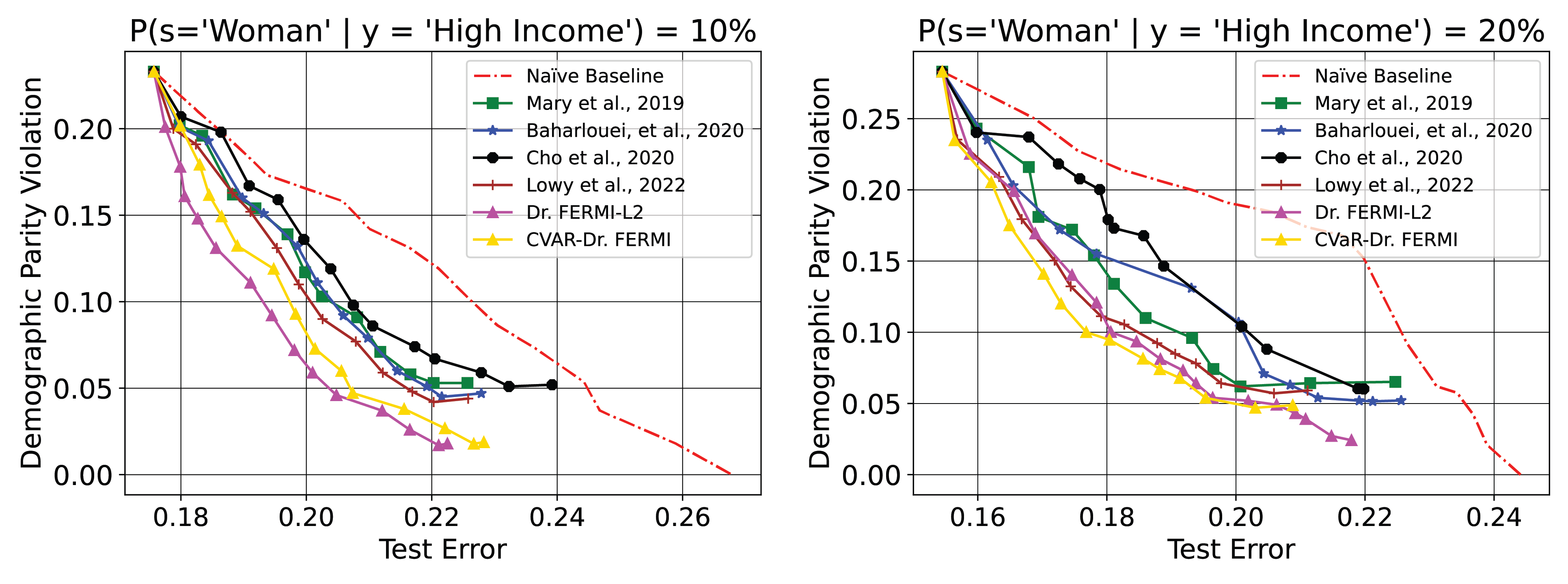
6.1 Modifying Benchmark Datasets to Contain Hybrid Distribution Shifts
Standard benchmark datasets in algorithmic fairness, such as Adult, German Credit, and COMPAS (Dua and Graff, 2017), include test and training data that follow the same distribution. To impose distribution shifts, we choose a subset of the test data to generate datasets containing demographic and label shifts. The demographic shift is the change in the population of different sensitive sub-populations from the source and the target distributions, i.e., . Similarly, the label shift means . The Adult training (and test) data has the following characteristics:
We generate two different test datasets containing distribution shifts where the probability is and (by undersampling and oversampling high-income women). We train the model on the original dataset and evaluate the performance and fairness (in terms of demographic parity violation) on two newly generated datasets in Figure 1.
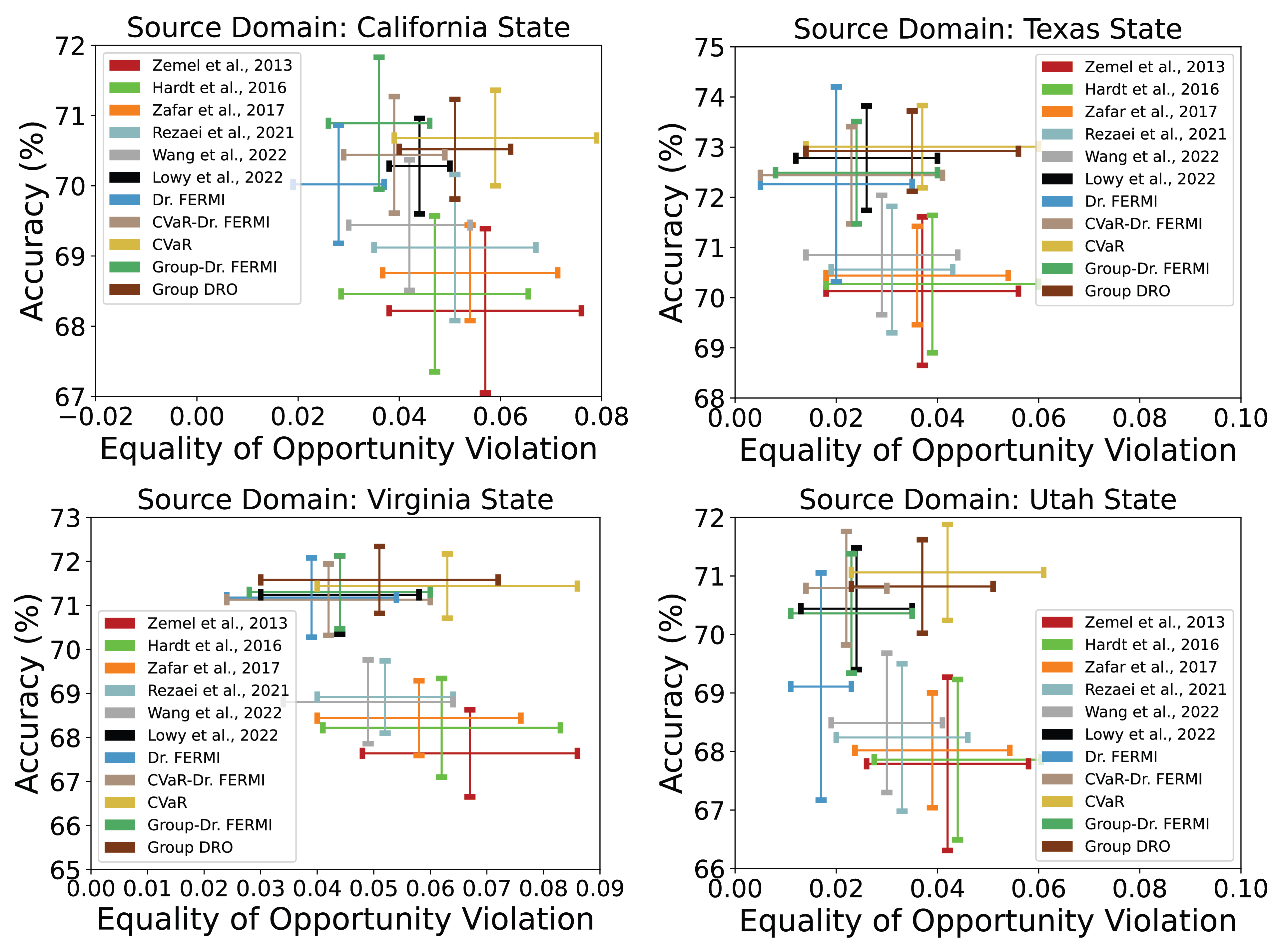
6.2 Robustness Against Distribution Shift in Real Datasets
While the original Adult dataset (Dua and Graff, 2017) has no considerable distribution shift, a relatively new dataset ACS-Income (Ding et al., 2021) designed based on the US census records contains natural distribution shifts since we can choose different US states as source and target datasets. The underlying task defined on the dataset is to predict whether a given person is high-income or low-income. The sensitive attributes are gender and race. Using this data, we perform experiments on binary and non-binary sensitive attribute cases. In the binary setting, we only consider gender as the sensitive attribute (in the dataset there are only two genders). In the non-binary case, we have four different sensitive groups: White-Male, White-Female, Black-Male, and Black-Female (a combination of race and gender). One can observe that and have large fluctuations over different states. Thus, these datasets, as mentioned in the paper (Ding et al., 2021), naturally contain the distribution shift with respect to different states.
In Figure 2, we apply Hardt Post-Processing approach (Hardt et al., 2016), Zemel Pre-processing method (Zemel et al., 2013), FERMI (Lowy et al., 2022), Robust Log-Loss under covariate shift (Rezaei et al., 2021), Curvature matching with MMD (Wang et al., 2022), and our distributionally robust method under norm for three accuracy variations (Dr. FERMI, CVaR-Dr. FERMI, and Group-Dr. FERMI), on the new adult (ACS-Income) dataset (Ding et al., 2021). The methods are trained on a single state (California, Texas, Utah, and Virginia) and evaluated/tested on all states in terms of prediction accuracy and fairness violation under the equality of opportunity notion. We chose California and Texas in accordance with other papers in the literature as two datasets with a large number of samples. Further, we chose Utah and Virginia as the two states with the highest and lowest initial equality of opportunity violations.
Each method’s horizontal and vertical range in Figure 2 denote -th and -th percentiles of accuracy and fairness violations across states, respectively. Thus, if a line is wider, it is less robust to the distribution shift. Ideally, we prefer models whose corresponding curves are on the upper-left side of the plot. Figure 2 shows that Dr. FERMI with uncertainty ball has a better robust, fair performance than other approaches among states when the training (in-distribution) dataset is either of the four aforementioned states. When maintaining more accuracy is a priority, one can use CVaR or Group DRO as the objective function for the accuracy part instead of the ERM. As a note, we can see that learning the model on a dataset with a more initial fairness gap (Utah) leads to a better generalization in terms of fairness violation, while learning on datasets with a less fairness gap (Virginia) leads to poorer fairness in the test phase.
6.3 Handling Distribution Shift in Non-Binary Case
We run different versions of Dr. FERMI alongside Mary et al. (2019), Baharlouei et al. (2019), Cho et al. (2020), and Lowy et al. (2022) as the baselines supporting multiple sensitive attributes. The algorithms are executed on the ACS PUMS (Ding et al., 2021) dataset with gender and race as the sensitive attributes. The accuracy and equality of opportunity violations are calculated on different datasets, and the average is reported in Table 1. Training is done on California data. Dr. FERMI under ball has the best performance in terms of average fairness violation across states. For robust accuracy, we suggest using CVaR for robustifying the accuracy. Note that, in all cases, the training equality of opportunity violation is set to 0.02 for all methods in the table.
Evaluation of Stochastic DR ERMI: batch sizes. By reducing the batch size from full-batch to small batches, we observed that our algorithm’s performance remains nearly the same, while other benchmarks’ performance varies significantly. Further, we report the time and memory consumption of Dr. FERMI and other benchmarks on the experiment presented in Table 1. The results of these experiments are available in Appendix J.
| Method | Tr Accuracy | Test Accuracy | Test EO Violation |
| Mary et al., 2019 | 71.41% | 68.35% | 0.1132 |
| Cho et al., 2020 | 71.84% | 68.91% | 0.1347 |
| Baharlouei et al., 2020 | 72.77% | 69.44% | 0.0652 |
| Lowy et al., 2022 | 73.81% | 70.22% | 0.0512 |
| Dr. FERMI- | 73.45% | 70.09% | 0.0392 |
| Dr. FERMI- | 73.12% | 69.71% | 0.0346 |
| Dr. FERMI- | 73.57% | 69.88% | \ul0.0359 |
| CVaR-Dr. FERMI- | 74.21% | 70.94% | 0.0471 |
| CVaR-Dr. FERMI- | 73.84% | 70.26% | 0.0429 |
| CVaR-Dr. FERMI- | \ul73.92% | \ul70.45% | 0.0466 |
References
- Abdel-Hamid et al. [2014] O. Abdel-Hamid, A.-r. Mohamed, H. Jiang, L. Deng, G. Penn, and D. Yu. Convolutional neural networks for speech recognition. IEEE/ACM Transactions on audio, speech, and language processing, 22(10):1533–1545, 2014.
- Act [1964] C. R. Act. Civil rights act of 1964. Title VII, Equal Employment Opportunities, 1964.
- An et al. [2022] B. An, Z. Che, M. Ding, and F. Huang. Transferring fairness under distribution shifts via fair consistency regularization. arXiv preprint arXiv:2206.12796, 2022.
- Angwin et al. [2016] J. Angwin, J. Larson, S. Mattu, and L. Kirchner. Machine bias. In Ethics of Data and Analytics, pages 254–264. Auerbach Publications, 2016.
- Baharlouei et al. [2019] S. Baharlouei, M. Nouiehed, A. Beirami, and M. Razaviyayn. Rényi fair inference. In International Conference on Learning Representations, 2019.
- Baharlouei et al. [2023] S. Baharlouei, K. Ogudu, S.-c. Suen, and M. Razaviyayn. RIFLE: Imputation and robust inference from low order marginals. Transactions on Machine Learning Research, 2023. ISSN 2835-8856. URL https://openreview.net/forum?id=oud7Ny0KQy.
- Ben-David et al. [2006] S. Ben-David, J. Blitzer, K. Crammer, and F. Pereira. Analysis of representations for domain adaptation. Advances in neural information processing systems, 19, 2006.
- Ben-David et al. [2010] S. Ben-David, J. Blitzer, K. Crammer, A. Kulesza, F. Pereira, and J. W. Vaughan. A theory of learning from different domains. Machine learning, 79(1):151–175, 2010.
- Blanchet et al. [2019] J. Blanchet, Y. Kang, K. Murthy, and F. Zhang. Data-driven optimal transport cost selection for distributionally robust optimization. In 2019 winter simulation conference (WSC), pages 3740–3751. IEEE, 2019.
- Buolamwini and Gebru [2018] J. Buolamwini and T. Gebru. Gender shades: Intersectional accuracy disparities in commercial gender classification. In Conference on fairness, accountability and transparency, pages 77–91. PMLR, 2018.
- Cho et al. [2020] J. Cho, G. Hwang, and C. Suh. A fair classifier using kernel density estimation. Advances in neural information processing systems, 33:15088–15099, 2020.
- Creager et al. [2019] E. Creager, D. Madras, J.-H. Jacobsen, M. Weis, K. Swersky, T. Pitassi, and R. Zemel. Flexibly fair representation learning by disentanglement. In International conference on machine learning, pages 1436–1445. PMLR, 2019.
- Dai and Brown [2020] J. Dai and S. M. Brown. Label bias, label shift: Fair machine learning with unreliable labels. In NeurIPS 2020 Workshop on Consequential Decision Making in Dynamic Environments, volume 12, 2020.
- Daskalakis et al. [2021] C. Daskalakis, S. Skoulakis, and M. Zampetakis. The complexity of constrained min-max optimization. In Proceedings of the 53rd Annual ACM SIGACT Symposium on Theory of Computing, pages 1466–1478, 2021.
- Delage and Ye [2010] E. Delage and Y. Ye. Distributionally robust optimization under moment uncertainty with application to data-driven problems. Operations research, 58(3):595–612, 2010.
- Devlin et al. [2018] J. Devlin, M.-W. Chang, K. Lee, and K. Toutanova. Bert: Pre-training of deep bidirectional transformers for language understanding. arXiv preprint arXiv:1810.04805, 2018.
- Ding et al. [2021] F. Ding, M. Hardt, J. Miller, and L. Schmidt. Retiring adult: New datasets for fair machine learning. Advances in Neural Information Processing Systems, 34:6478–6490, 2021.
- Donini et al. [2018] M. Donini, L. Oneto, S. Ben-David, J. S. Shawe-Taylor, and M. Pontil. Empirical risk minimization under fairness constraints. Advances in Neural Information Processing Systems, 31, 2018.
- Du and Wu [2021] W. Du and X. Wu. Fair and robust classification under sample selection bias. In Proceedings of the 30th ACM International Conference on Information & Knowledge Management, pages 2999–3003, 2021.
- Dua and Graff [2017] D. Dua and C. Graff. UCI machine learning repository, 2017. URL http://archive.ics.uci.edu/ml.
- Dwork et al. [2012] C. Dwork, M. Hardt, T. Pitassi, O. Reingold, and R. Zemel. Fairness through awareness. In Proceedings of the 3rd innovations in theoretical computer science conference, pages 214–226, 2012.
- Fang et al. [2020] T. Fang, N. Lu, G. Niu, and M. Sugiyama. Rethinking importance weighting for deep learning under distribution shift. Advances in Neural Information Processing Systems, 33:11996–12007, 2020.
- Gao and Kleywegt [2017] R. Gao and A. J. Kleywegt. Distributionally robust stochastic optimization with dependence structure. arXiv preprint arXiv:1701.04200, 2017.
- Gebelein [1941] H. Gebelein. Das statistische problem der korrelation als variations-und eigenwertproblem und sein zusammenhang mit der ausgleichsrechnung. ZAMM-Journal of Applied Mathematics and Mechanics/Zeitschrift für Angewandte Mathematik und Mechanik, 21(6):364–379, 1941.
- Grari et al. [2019] V. Grari, B. Ruf, S. Lamprier, and M. Detyniecki. Fairness-aware neural r’eyni minimization for continuous features. arXiv preprint arXiv:1911.04929, 2019.
- Hardt et al. [2016] M. Hardt, E. Price, and N. Srebro. Equality of opportunity in supervised learning. Advances in neural information processing systems, 29, 2016.
- Hirschfeld [1935] H. O. Hirschfeld. A connection between correlation and contingency. In Mathematical Proceedings of the Cambridge Philosophical Society, volume 31, pages 520–524. Cambridge University Press, 1935.
- Jin et al. [2020] C. Jin, P. Netrapalli, and M. Jordan. What is local optimality in nonconvex-nonconcave minimax optimization? In International conference on machine learning, pages 4880–4889. PMLR, 2020.
- Jing et al. [2021] T. Jing, B. Xu, and Z. Ding. Towards fair knowledge transfer for imbalanced domain adaptation. IEEE Transactions on Image Processing, 30:8200–8211, 2021.
- Kale et al. [2022] S. Kale, J. D. Lee, C. De Sa, A. Sekhari, and K. Sridharan. From gradient flow on population loss to learning with stochastic gradient descent. arXiv preprint arXiv:2210.06705, 2022.
- Khalafi and Boob [2023] M. Khalafi and D. Boob. Accelerated primal-dual methods for convex-strongly-concave saddle point problems. In A. Krause, E. Brunskill, K. Cho, B. Engelhardt, S. Sabato, and J. Scarlett, editors, Proceedings of the 40th International Conference on Machine Learning, volume 202 of Proceedings of Machine Learning Research, pages 16250–16270. PMLR, 23–29 Jul 2023.
- Kim et al. [2019] M. P. Kim, A. Ghorbani, and J. Zou. Multiaccuracy: Black-box post-processing for fairness in classification. In Proceedings of the 2019 AAAI/ACM Conference on AI, Ethics, and Society, pages 247–254, 2019.
- Krizhevsky et al. [2017] A. Krizhevsky, I. Sutskever, and G. E. Hinton. Imagenet classification with deep convolutional neural networks. Communications of the ACM, 60(6):84–90, 2017.
- Kuhn et al. [2019] D. Kuhn, P. M. Esfahani, V. A. Nguyen, and S. Shafieezadeh-Abadeh. Wasserstein distributionally robust optimization: Theory and applications in machine learning. In Operations research & management science in the age of analytics, pages 130–166. Informs, 2019.
- Lechner et al. [2021] T. Lechner, S. Ben-David, S. Agarwal, and N. Ananthakrishnan. Impossibility results for fair representations. arXiv preprint arXiv:2107.03483, 2021.
- Lee et al. [2019] J. D. Lee, I. Panageas, G. Piliouras, M. Simchowitz, M. I. Jordan, and B. Recht. First-order methods almost always avoid strict saddle points. Mathematical programming, 176(1):311–337, 2019.
- Levy et al. [2020] D. Levy, Y. Carmon, J. C. Duchi, and A. Sidford. Large-scale methods for distributionally robust optimization. Advances in Neural Information Processing Systems, 33:8847–8860, 2020.
- Li et al. [2019] Z. Li, K. Kamnitsas, and B. Glocker. Overfitting of neural nets under class imbalance: Analysis and improvements for segmentation. In International Conference on Medical Image Computing and Computer-Assisted Intervention, pages 402–410. Springer, 2019.
- Lin et al. [2022] F. Lin, X. Fang, and Z. Gao. Distributionally robust optimization: A review on theory and applications. Numerical Algebra, Control & Optimization, 12(1):159, 2022.
- Lohia et al. [2019] P. K. Lohia, K. N. Ramamurthy, M. Bhide, D. Saha, K. R. Varshney, and R. Puri. Bias mitigation post-processing for individual and group fairness. In Icassp 2019-2019 ieee international conference on acoustics, speech and signal processing (icassp), pages 2847–2851. IEEE, 2019.
- Lowy et al. [2022] A. Lowy, S. Baharlouei, R. Pavan, M. Razaviyayn, and A. Beirami. A stochastic optimization framework for fair risk minimization. Transaction on Machine Learning Research (TMLR), 2022.
- Mary et al. [2019] J. Mary, C. Calauzenes, and N. El Karoui. Fairness-aware learning for continuous attributes and treatments. In International Conference on Machine Learning, pages 4382–4391. PMLR, 2019.
- Moreno-Torres et al. [2012] J. G. Moreno-Torres, T. Raeder, R. Alaiz-Rodríguez, N. V. Chawla, and F. Herrera. A unifying view on dataset shift in classification. Pattern recognition, 45(1):521–530, 2012.
- Narayanan [2018] A. Narayanan. Translation tutorial: 21 fairness definitions and their politics. In Proc. Conf. Fairness Accountability Transp., New York, USA, volume 1170, page 3, 2018.
- Nazari et al. [2023] A. Nazari, Y. Huang, R. Samanta, A. Radhakrishna, and M. Raghothaman. Explainable program synthesis by localizing specifications. Proceedings of the ACM on Programming Languages, 2023.
- Nemirovski et al. [2009] A. Nemirovski, A. Juditsky, G. Lan, and A. Shapiro. Robust stochastic approximation approach to stochastic programming. SIAM Journal on optimization, 19(4):1574–1609, 2009.
- Oneto et al. [2020] L. Oneto, M. Donini, G. Luise, C. Ciliberto, A. Maurer, and M. Pontil. Exploiting mmd and sinkhorn divergences for fair and transferable representation learning. Advances in Neural Information Processing Systems, 33:15360–15370, 2020.
- Polyak [1990] B. T. Polyak. New stochastic approximation type procedures. Automat. i Telemekh, 7(98-107):2, 1990.
- Prost et al. [2019] F. Prost, H. Qian, Q. Chen, E. H. Chi, J. Chen, and A. Beutel. Toward a better trade-off between performance and fairness with kernel-based distribution matching. arXiv preprint arXiv:1910.11779, 2019.
- Rahimian and Mehrotra [2019] H. Rahimian and S. Mehrotra. Distributionally robust optimization: A review. arXiv preprint arXiv:1908.05659, 2019.
- Razaviyayn et al. [2020] M. Razaviyayn, T. Huang, S. Lu, M. Nouiehed, M. Sanjabi, and M. Hong. Nonconvex min-max optimization: Applications, challenges, and recent theoretical advances. IEEE Signal Processing Magazine, 37(5):55–66, 2020.
- Recht et al. [2018] B. Recht, R. Roelofs, L. Schmidt, and V. Shankar. Do cifar-10 classifiers generalize to cifar-10? arXiv preprint arXiv:1806.00451, 2018.
- Recht et al. [2019] B. Recht, R. Roelofs, L. Schmidt, and V. Shankar. Do imagenet classifiers generalize to imagenet? In International Conference on Machine Learning, pages 5389–5400. PMLR, 2019.
- Rényi [1959] A. Rényi. On measures of dependence. Acta mathematica hungarica, 10(3-4):441–451, 1959.
- Rezaei et al. [2020] A. Rezaei, R. Fathony, O. Memarrast, and B. Ziebart. Fairness for robust log loss classification. In Proceedings of the AAAI Conference on Artificial Intelligence, volume 34, pages 5511–5518, 2020.
- Rezaei et al. [2021] A. Rezaei, A. Liu, O. Memarrast, and B. D. Ziebart. Robust fairness under covariate shift. In Proceedings of the AAAI Conference on Artificial Intelligence, volume 35, pages 9419–9427, 2021.
- Rockafellar et al. [2000] R. T. Rockafellar, S. Uryasev, et al. Optimization of conditional value-at-risk. Journal of risk, 2:21–42, 2000.
- Roh et al. [2020] Y. Roh, K. Lee, S. Whang, and C. Suh. Fr-train: A mutual information-based approach to fair and robust training. In International Conference on Machine Learning, pages 8147–8157. PMLR, 2020.
- Sagawa et al. [2019] S. Sagawa, P. W. Koh, T. B. Hashimoto, and P. Liang. Distributionally robust neural networks for group shifts: On the importance of regularization for worst-case generalization. arXiv preprint arXiv:1911.08731, 2019.
- Saravani et al. [2021] S. M. Saravani, I. Ray, and I. Ray. Automated identification of social media bots using deepfake text detection. In International Conference on Information Systems Security, pages 111–123. Springer, 2021.
- Schrouff et al. [2022] J. Schrouff, N. Harris, O. Koyejo, I. Alabdulmohsin, E. Schnider, K. Opsahl-Ong, A. Brown, S. Roy, D. Mincu, C. Chen, et al. Maintaining fairness across distribution shift: do we have viable solutions for real-world applications? arXiv preprint arXiv:2202.01034, 2022.
- Shapiro et al. [2021] A. Shapiro, D. Dentcheva, and A. Ruszczynski. Lectures on stochastic programming: modeling and theory. SIAM, 2021.
- Singh et al. [2019] H. Singh, R. Singh, V. Mhasawade, and R. Chunara. Fair predictors under distribution shift. In NeurIPS Workshop on Fair ML for Health, 2019.
- Sion [1958] M. Sion. On general minimax theorems. Pacific Journal of mathematics, 8(1):171–176, 1958.
- Tan et al. [2020] M. Tan, R. Pang, and Q. V. Le. Efficientdet: Scalable and efficient object detection. In Proceedings of the IEEE/CVF conference on computer vision and pattern recognition, pages 10781–10790, 2020.
- Taskesen et al. [2020] B. Taskesen, V. A. Nguyen, D. Kuhn, and J. Blanchet. A distributionally robust approach to fair classification. arXiv preprint arXiv:2007.09530, 2020.
- Tzeng et al. [2014] E. Tzeng, J. Hoffman, N. Zhang, K. Saenko, and T. Darrell. Deep domain confusion: Maximizing for domain invariance. arXiv preprint arXiv:1412.3474, 2014.
- Vaithilingam et al. [2022] P. Vaithilingam, T. Zhang, and E. L. Glassman. Expectation vs. experience: Evaluating the usability of code generation tools powered by large language models. In Chi conference on human factors in computing systems extended abstracts, pages 1–7, 2022.
- Wang et al. [2022] H. Wang, J. Hong, J. Zhou, and Z. Wang. How robust is your fairness? evaluating and sustaining fairness under unseen distribution shifts. arXiv preprint arXiv:2207.01168, 2022.
- Wiesemann et al. [2014] W. Wiesemann, D. Kuhn, and M. Sim. Distributionally robust convex optimization. Operations Research, 62(6):1358–1376, 2014.
- Witsenhausen [1975] H. S. Witsenhausen. On sequences of pairs of dependent random variables. SIAM Journal on Applied Mathematics, 28(1):100–113, 1975.
- Xu et al. [2009] H. Xu, C. Caramanis, and S. Mannor. Robustness and regularization of support vector machines. Journal of machine learning research, 10(7), 2009.
- Zafar et al. [2017a] M. B. Zafar, I. Valera, M. Rodriguez, K. Gummadi, and A. Weller. From parity to preference-based notions of fairness in classification. Advances in Neural Information Processing Systems, 30, 2017a.
- Zafar et al. [2017b] M. B. Zafar, I. Valera, M. G. Rogriguez, and K. P. Gummadi. Fairness constraints: Mechanisms for fair classification. In Artificial intelligence and statistics, pages 962–970. PMLR, 2017b.
- Zemel et al. [2013] R. Zemel, Y. Wu, K. Swersky, T. Pitassi, and C. Dwork. Learning fair representations. In International conference on machine learning, pages 325–333. PMLR, 2013.
- Zhou et al. [2021] C. Zhou, X. Ma, P. Michel, and G. Neubig. Examining and combating spurious features under distribution shift. In International Conference on Machine Learning, pages 12857–12867. PMLR, 2021.
- Zymler et al. [2013] S. Zymler, D. Kuhn, and B. Rustem. Distributionally robust joint chance constraints with second-order moment information. Mathematical Programming, 137(1):167–198, 2013.
Appendix A Proof of Theorem 1
Let and be the singular value decompositions of matrices and respectively. We aim to solve the following optimization problem:
| (16) |
Since and are unitary matrices (), we have . Therefore, Problem (16) is equivalent to:
| (17) |
a) If , we aim to solve the following maximization problem:
| (18) |
Let and be the vectorized forms of and respectively. Therefore, the above problem is equivalent to the following:
| (19) |
Without loss of generality, assume that . We claim the solution to this problem is obtained by putting all budgets to the largest entry of (, and ). To arrive at a contradiction, assume that there exists an optimal solution such that and such that . We claim a solution with and has a higher objective value function:
Thus, with proof by contradiction, we have . Similarly for other ’s such that , if the optimal , then . Hence, the claim that the optimal solution to Problem (19) is obtained by putting to the largest entry is true. Note that the largest singular value of is always . We also consider the same constraint on matrix (this is a practical assumption since the actual matrix generated by , the ground-truth joint distribution of data in the test domain, has the largest singular value equal 1). Thus, to maximize the summation of singular values, we put all available budgets to the second-largest singular value. Therefore, the optimal solution to Problem (18) is , which is the desired result in Theorem 1 part a.
b) If , we require to solve the following maximization problem:
| (20) |
Assume that and Thus, Problem (20) is equivalent to:
| (21) |
Note that:
Setting , we can achieve to the maximum value without violating the constraints in (21). Therefore, the optimal solution to Problem (20) is which is . Therefore, Problem (20) is equivalent to:
| (22) |
which gives us the desired result in Theorem 1 part b.
c) In the case of , we seek to solve:
| (23) |
where the uncertainty set is defined on the singular values of the matrix . We can add to each singular value of the matrix independently to maximize the above problem. In that case, the optimal solution is , which is the desired result presented in Theorem 1.
Appendix B Proof of Theorem 3
First, note that there exists such that . To see why, we choose such that outputs uniformly at random between zero and one independent of . Thus, is independent of the sensitive attribute . By the definition of the Exponential Rényi Mutual Information (ERMI), , since and are independent. Assume that is the optimal solution of Problem Dr. FERMI for the given and . Since, the is the optimizer of (Dr. FERMI), we have:
| (24) |
The equality holds, since the is zero. Therefore:
| (25) |
Since the cross-entropy loss is always greater than or equal to zero, we have:
Further, assume that the loss value at point . Thus:
| (26) |
Therefore, if we choose , we have
| (27) |
We showed the above inequality for arbitrary choice of . Next, we choose such that . Note that according to Witsenhausen [1975], the largest singular value of the matrix is one. As a result, the size of all eigenvalues of matrices and are less than or equal to . Therefore, by choice of large enough , the distance of the vectors of eigenvalues for and is within . Hence:
According to Lowy et al. [2022, Lemma 3], the exponential Rényi Mutual Information is an upper bound for fairness violation (demographic parity violation). Thus:
which completes the proof.
Appendix C Proof of Lemma 4
First, we show that for any :
| (28) |
Let . Since , the function is strictly convex with respect to . Thus, the minimizer is unique. The minimizer of can be obtained by setting the derivative to zero with respect to :
Therefore, the optimal value can be obtained by plugging in into :
that proves (28). Based on [Lowy et al., 2022, Lemma 1],
| (29) |
where is given by Equation (15). Thus Problem (10) can be written as:
| (30) |
Applying Equation (28) to , we have:
| (31) |
Combining (30) and (31), Problem (10) can be reformulated as:
| (32) |
Note that the maximization problem with respect to is concave due to the concavity of , and the minimization problem with respect to is convex on . To switch the minimum and maximum terms, we need to have boundedness on the parameters of the minimization problem. Obviously, is bounded below by . Further, note that the optimal satisfies the following condition due to the first-order stationarity condition:
Since is the reformulation of and the latter term is the summation of all singular values, it is always greater than or equal to (since the largest singular value equals ). As a result . Therefore, it is bounded from above as well. Thus, we can switch the maximization and minimization problems in (C) due to the minimax theorem [Sion, 1958]. Hence, Problem (10) is equivalent to
which is precisely Problem (14).
Appendix D Significance and Limitations of Theorem 3
The obtained result is based on the two crucial properties of (7) formulation: First, bounding the ERMI between sensitive attributes and predictions results in bounding the demographic parity violation. Second, the uncertainty sets characterized by balls around the matrix can be chosen such that the current distribution shift lies within the uncertainty ball. In that sense, the proposed framework is less restrictive than the aforementioned related works that only focus on a specific type of shift, such as demographic, covariate, or label shifts. Note that Theorem 3 only provides a generalization guarantee on the unseen data for the model’s fairness. Therefore, it does not guarantee any level of accuracy on the test data. An open question is whether optimizing the loss function in (10) leads to a solution with both Fairness and Accuracy guarantees on the unseen data. Such a problem is challenging even in the case of generalizability of non-convex trained models when no fairness concerns are considered. Further, the satisfaction of at each iteration as a necessary condition depends on the choice of . A large distance between and can lead to larger , and therefore the poor performance of the trained model in terms of accuracy as the compensation for promoting fairness.
Appendix E Derivation of Algorithm 1 and Details on Computing Gradients
Algorithm 1 requires to update the probability matrices and after updating . Assume that the output of the classification model is a probability vector (logits in neural networks or logistic regression) where the probability of assigning label to the data point is . Note that . One can compute the elements of probability matrices as follows:
| (33) | |||
| (34) |
As a note, and it is constant through the algorithm.
Appendix F Stochastic Gradient Descent Ascent (SGDA) Algorithms For (Dr. FERMI)
This section proposes the stochastic algorithm for solving (Dr. FERMI) under the norm ball as the uncertainty set. Then, we show the algorithm finds a stationary solution to the problem in . As mentioned in Section 4.2, (Dr. FERMI) can be rewritten as:
Since the objective function is represented as an average/expectation over data points, the gradient vector with respect to evaluated for a given batch of data is an unbiased estimator of the gradient with respect to all data points. Further, the problem is strongly concave with respect to the matrix . Therefore, a standard stochastic gradient descent ascent (SGDA) algorithm will find a stationary solution to the problem. Algorithm 2 describes the procedure of optimizing (14).
Proposition 5
The proof is based on the following assumptions:
-
•
-
•
for every iteration of the algorithm.
-
•
The loss function and the probabilistic output are Lipschitz continuous with the Lipschitz constant .
-
•
The loss function and the probabilistic output are -smooth, meaning that their gradients are Lipschitz continuous with the Lipschitz constant .
Remark 6
Note that the first two assumptions are true in practice. Because we assume at least one sample from each sensitive group should be available in the training data. Further, the probability of predicting any label in every iteration should not be zero. In our experiments, such an assumption always holds. If, for some extreme cases, one probability goes to zero, one can add a small perturbation to to avoid the exact zero probability. The third and fourth assumptions are standard in the convergence of iterative method proofs, and they hold for loss functions such as cross-entropy and mean-squared loss over bounded inputs.
Proof
Define , which means is obtained by adding the parameter to vector . In that case, Algorithm 2 can be seen as one step of gradient descent to and one step of projected gradient ascent to . Note that, although the maximization problem is originally unconstrained, we are required to apply the projection to the set to ensure the Lipschitz continuity and the boundedness of the variance of the gradient estimator. The convergence of Algorithm 2 to an -stationary solution of Problem 10 in is the direct result of Theorem 3 in Lowy et al. [2022].
Appendix G Convergence of Algorithm 1
Since we solve the maximization problem in (9) in closed form (see lines 5 and 6 in Algorithm 1), as an immediate result of Theorem 27 in Jin et al. [2020], Algorithm 1 converges to a stationary solution of Problem (9) in . Note that, although the problem is non-convex non-concave, we have a max oracle (we can exactly compute the solution to the maximum problem in closed form).
Appendix H Full-Batch Algorithms for Problem (10) and Problem (11)
To solve Problem 10, we use the following gradient descent-ascent (GDA) approach:
To solve Problem (11), we use the following algorithm:
Appendix I Algorithms for CVaR-Dr. CVaR and GROUP-Dr. FERMI
By a simple modification of Algorithm 1, one can derive convergent algorithms to the stationary points of (CVaR-Dr. FERMI) and (Group-Dr. FERMI). Note that the maximization step at each iteration remains the same. The only change is in the minimization part. Instead of minimizing with respect to , we need to update the extra parameter as an optimization problem using (sub-)gradient descent. Algorithm 5 describes the procedure of optimizing (CVaR-Dr. FERMI). At each iteration, we apply one step of (sub-)gradient descent to and and then update and in closed form.
Similarly, one can optimize (Group-Dr. FERMI) by applying gradient descent to the as in Algorithm 1 and the group DRO parameters as in Algorithm 1 in Sagawa et al. [2019] and then applying and in the closed form at each iteration.
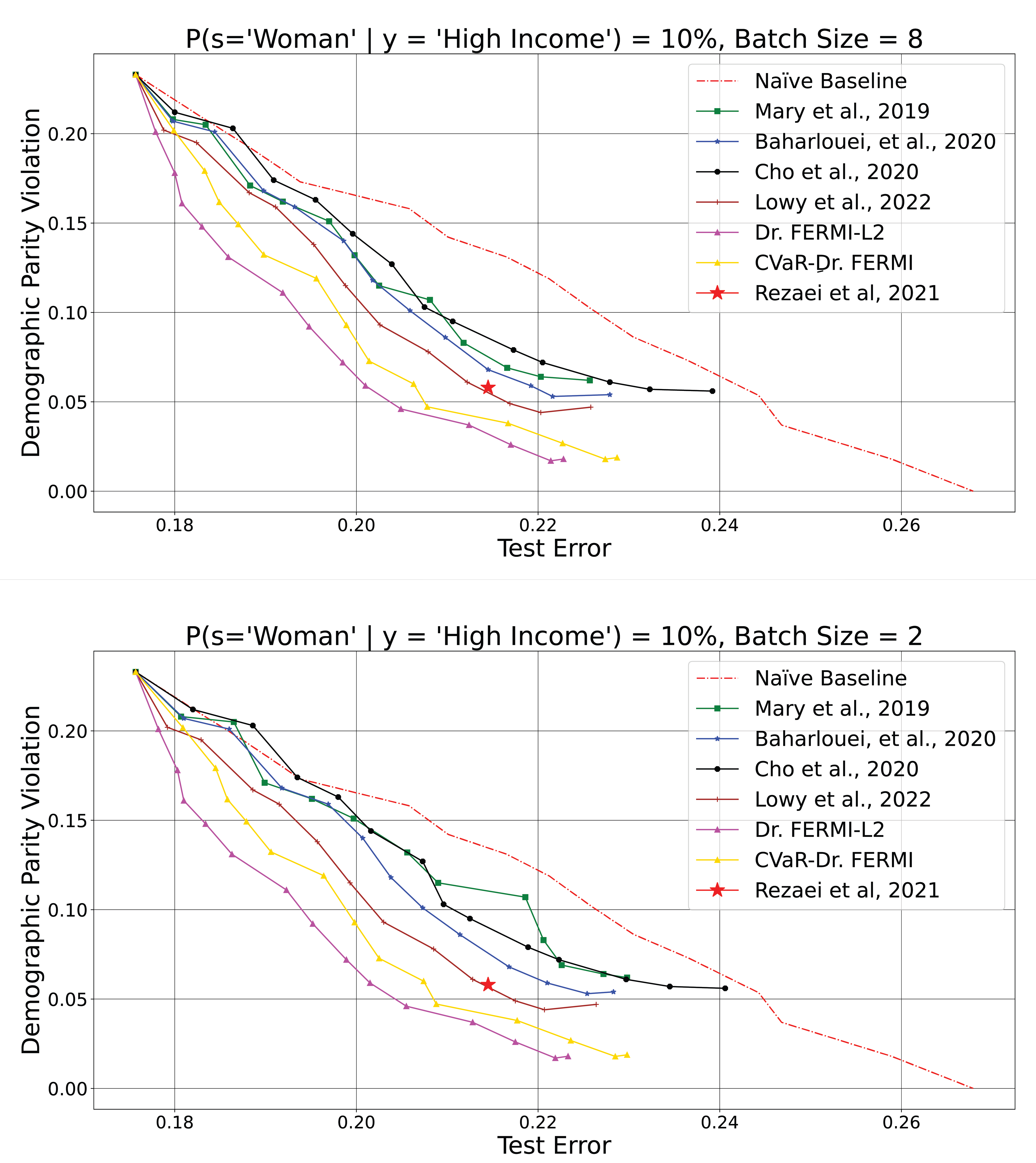
Appendix J Performance of Stochastic DR ERMI
In this section, we evaluate Algorithm 2 for different batch sizes. To this end, we learn fair models with different batch sizes on the adult dataset where the minority group is under-represented. We compare Algorithm 2 to [Lowy et al., 2022], [Baharlouei et al., 2019], [Rezaei et al., 2021], [Mary et al., 2019], and [Cho et al., 2020] as the baselines supporting stochastic updates. Since the gradient estimator in Algorithm 2 is unbiased, the performance of Algorithm 2 remains consistently well for different batch sizes. However, by reducing the batch size, other methods (except Lowy et al. [2022]) fail to keep their initial performance on the full batch setting. Comparing our approach and Lowy et al. [2022], we achieve better generalization in terms of the fairness-accuracy tradeoff for different batch sizes.
Appendix K More Details on Experiments
This section presents a more detailed version of Table 1 with added accuracy and fairness standard deviations among states.
| Method | Tr Accuracy | Test Accuracy | Test EO Violation |
| Mary et al., 2019 | |||
| Cho et al., 2020 | |||
| Baharlouei et al., 2020 | |||
| Lowy et al., 2022 | |||
| Dr. FERMI- | |||
| Dr. FERMI- | |||
| Dr. FERMI- | \ul0.0359 | ||
| CVaR-Dr. FERMI- | |||
| CVaR-Dr. FERMI- | |||
| CVaR-Dr. FERMI- | \ul73.92 | \ul70.45 |
Further, to show the memory efficiency of Dr. FERMI, we report the memory consumption, the execution time
| Method | Memory Consumption | Training Time |
|---|---|---|
| CVaR Dr. FERMI | \ul<800 Mb | 783 (s) |
| Dr. FERMI | <800 Mb | 692 (s) |
| Lowy et al, 2022 | <800 Mb | 641 (s) |
| Cho et al., 2021 | 1.21 Gb | 3641 (s) |
| Rezaei et al., 2021 | 1.59 Gb | 3095 (s) |
| Baharlouei, et al., 2020 | <900 Mb | 2150 (s) |
| Mary, et al., 2019 | <1.43 Gb | 1702 (s) |
Appendix L Hyper-Parameter Tuning
DP-FERMI has two hyper-parameters and . Further, the presented algorithms in the paper have a step-size (learning rate) , and the number of iterations . We use and in the code. These values are obtained by changing and over different values in different runs on ACS PUMS [Ding et al., 2021] data. We consider two scenarios for tuning and . If a sample of data from the target domain is available for the validation, we reserve that data as the validation set to choose the optimal and . In the second scenario, when no data from the target domain is provided, one can rely on the -fold cross-validation on the source data. A more resilient approach is to create the validation dataset by oversampling the minority groups. Based on this idea, we do weighted sampling based on the population of sensitive groups (oversampling from minorities), and then, we choose the optimal and as in scenario .
Appendix M Limitations
In this paper, we address the fair empirical risk minimization in the presence of the distribution shift by handling the distribution shift of the target domain for the fairness and accuracy parts separately. As shown in Theorem 3, we can bound the fairness violation of the target domain with the proper choice of hyper-parameters. However, the proposed framework has several limitations. First, the defined uncertainty set for the fairness term is limited to norm balls (in certain variables) and the Exponential Rényi Mutual Information (ERMI) as the measure of fairness. Second, the presented guarantee is just for the fairness violation and does not offer any guarantee for the fairness-accuracy tradeoff. Moreover, the guarantees are for the global optimal solutions, which may not be possible to compute due to the nonconvexity of the problem.
Appendix N Broader Impacts
The emergence of large-scale machine learning models and artificial intelligence tools has brought about a pressing need to ensure the deployment of safe and reliable models. Now, more than ever, it is crucial to address the challenges posed by distribution shifts and strive for fairness in machine learning. This paper presents a comprehensive framework that tackles the deployment of large-scale fair machine learning models, offering provably convergent stochastic algorithms that come with statistical guarantees on the fairness of the models in the target domain.
While it is important to note that our proposed algorithms may not provide an all-encompassing solution for every application, we believe that sharing our research findings with the broader community will positively impact society. By publishing and disseminating our work, we hope to contribute to the ongoing discourse on fairness in machine learning and foster a collaborative environment for further advancements in this field. Moreover, the significance of our algorithms extends beyond the context of fairness. They can potentially be harnessed in a wide range of applications to enforce statistical independence between random variables in the presence of distribution shifts. This versatility underscores the potential impact of our research and its relevance across various domains.