Error estimate for regularized optimal transport problems
via Bregman divergence

Abstract.

Regularization by the Shannon entropy enables us to efficiently and approximately solve optimal transport problems on a finite set. This paper is concerned with regularized optimal transport problems via Bregman divergence. We introduce the required properties for Bregman divergences, provide a non-asymptotic error estimate for the regularized problem, and show that the error estimate becomes faster than exponentially.

1. Introduction

An optimal transport theory allows for measuring the difference between two probability measures. Innumerable applications of optimal transport theory include mathematics, physics, economics, statistics, computer science, and machine learning. This work focuses on the optimal transport theory on a finite set.

For $K\in\mathbb{N}$, define

$$\mathcal{P}_{K}:=\left\{z=(z_{k})\in\mathbb{R}^{K}\biggm{|}z_{k}\geq 0\ \text{for any }k,\ \sum_{k}z_{k}=1\right\}.$$

Here and hereafter, $k$ runs over $1,2,\ldots,K$. Fix $I,J\in\mathbb{N}$. Unless we indicate otherwise, $i$ and $j$ run over $1,2,\ldots,I$ and $1,2,\ldots,J$, respectively. For $x\in\mathcal{P}_{I}$ and $y\in\mathcal{P}_{J}$, define $x\otimes y\in\mathcal{P}_{I\times J}$ by

$$(x\otimes y)_{ij}:=x_{i}y_{j},$$

and set

(1.1) $$\Pi(x,y):=\left\{\Pi=(\pi_{ij})\in\mathcal{P}_{I\times J}\Biggm{|}\sum_{l=1}^{J}\pi_{il}=x_{i},\sum_{l=1}^{I}\pi_{lj}=y_{j}\ \text{for any }i,j\right\},$$

where we identify $\mathcal{P}_{I\times J}$ with a subset of $\mathbb{R}^{I\times J}$. An element in $\Pi(x,y)$ is called a transport plan between $x$ and $y$. Note that $\Pi(x,y)$ is a compact set, in particular, a convex polytope, and contains $x\otimes y$. Fix $C=(c^{ij})\in\mathbb{R}^{I\times J}$ and define a map $\langle C,\cdot\rangle:\mathcal{P}_{I\times J}\to\mathbb{R}$ by

$$\langle C,\Pi\rangle:=\sum_{i,j}c^{ij}\pi_{ij}.$$

Consider linear programs of the form

(1.2) $$\inf_{\Pi\in\Pi(x,y)}\langle C,\Pi\rangle,$$

which is a so-called optimal transport problem. Since the function $\langle C,\cdot\rangle$ is linear, in particular continuous on a compact set $\Pi(x,y)$, the problem (1.2) always admits a minimizer, but a minimizer is not necessarily unique. A minimizer of the problem (1.2) is called an optimal transport plan between $x$ and $y$.

In the context of the success of the regularized optimal transport problem by the Kullback–Leibler divergence, this paper considers a regularized optimal transport problem via Bregman divergence, which is a generalization of the Kullback–Leibler divergence through a strictly convex function.

Definition 1.1.

Let $U$ be a continuous, strictly convex function on $[0,1]$ with $U\in C^{1}((0,1])$. For $z,w\in\mathcal{P}_{K}$, the Bregman divergence associated with $U$ of $z$ with respect to $w$ is given by

$$D_{U}(z,w):=\sum_{k}d_{U}(z_{k},w_{k}),$$

where $d_{U}:[0,1]\times(0,1]\to\mathbb{R}$ is defined for $r\in[0,1]$ and $r_{0}\in(0,1]$ by

$$d_{U}(r,r_{0}):=U(r)-U(r_{0})-(r-r_{0})U^{\prime}(r_{0})$$

and is naturally extended as a function on $[0,1]\times[0,1]$ valued in $[0,\infty]$ (see Lemma 2.1).

For example, the Bregman divergence associated with $U(r)=r\log r$ reduces to the Kullback–Leibler divergence.

Let us consider a regularized problem of the form

(1.3) $$\inf_{\Pi\in\Pi(x,y)}\left(\langle C,\Pi\rangle+\varepsilon D_{U}(\Pi,x\otimes y)\right)\quad\text{for }\varepsilon>0.$$

By the continuity and strict convexity of $U$, $D_{U}(\cdot,x\otimes y)$ is continuous and strictly convex on a convex polytope $\Pi(x,y)$. Consequently, the problem (1.3) always admits a unique minimizer, denoted by $\Pi^{U}(C,x,y,\varepsilon)$. Then,

(1.4) $$\lim_{\varepsilon\downarrow 0}\langle C,\Pi^{U}(C,x,y,\varepsilon)\rangle=\inf_{\Pi\in\Pi(x,y)}\langle C,\Pi\rangle$$

holds (see Subsection 2.4). To give a quantitative error estimate of (1.4), we require the following two assumptions. See Subsections 2.1 and 2.3 to verify that the assumptions are reasonable.

Assumption 1.2.

$\Pi(x,y)\neq\operatorname*{argmin}_{\Pi\in\Pi(x,y)}\langle C,\Pi\rangle$.

Assumption 1.3.

Let $U\in C([0,1])\cap C^{1}((0,1])\cap C^{2}((0,1))$ satisfy $U^{\prime\prime}>0$ on $(0,1)$ and $\lim_{h\downarrow 0}U^{\prime}(h)=-\infty$. In addition, $r\mapsto rU^{\prime\prime}(r)$ is non-decreasing in $(0,1)$.

We introduce notions to describe our quantitative error estimate of (1.4).

Definition 1.4.

Let $U$ be a continuous, strictly convex function on $[0,1]$ with $U\in C^{1}((0,1])$. Define $\mathfrak{D}_{U}(x,y)$ for $x\in\mathcal{P}_{I}$ and $y\in\mathcal{P}_{J}$ by

(1.5) $$\mathfrak{D}_{U}(x,y)\coloneqq\sup_{\Pi\in\Pi(x,y)}D_{U}(\Pi,x\otimes y).$$

Definition 1.5.

The suboptimality gap of $x\in\mathcal{P}_{I}$ and $y\in\mathcal{P}_{J}$ with respect to $C\in\mathbb{R}^{I\times J}$ is defined by

(1.6) $$\Delta_{C}(x,y)\coloneqq\inf_{V^{\prime}\in V(x,y)\setminus\operatorname*{argmin}_{V\in V(x,y)}\langle C,V\rangle}\langle C,V^{\prime}\rangle-\inf_{V\in V(x,y)}\langle C,V\rangle,$$

where $V(x,y)$ is the set of vertices of $\Pi(x,y)$ and set $\inf\emptyset:=\infty$.

In Subsection 2.1, we verify $\mathfrak{D}_{U}(x,y),\Delta_{C}(x,y)\in(0,\infty)$ under Assumption 1.2. We also confirm in Subsection 2.2 that Definition 1.6 below is well-defined.

Definition 1.6.

Under Assumption 1.3, we denote by $e_{U}$ the inverse function of $U^{\prime}:(0,1]\to U^{\prime}((0,1])$. For $x\in\mathcal{P}_{I}$ and $y\in\mathcal{P}_{J}$, let $R_{U}(x,y)\in[1/2,1)$ satisfy

$$U^{\prime}(R_{U}(x,y))-U^{\prime}(1-R_{U}(x,y))=\mathfrak{D}_{U}(x,y),$$

which is uniquely determined. Define $\nu_{U}(x,y)\in\mathbb{R}$ by

(1.7) $$\nu_{U}(x,y):=\sup_{r\in(0,R_{U}(x,y)]}\left(U^{\prime}(1-r)+rU^{\prime\prime}(r)\right).$$

Our main result is as follows.

Theorem 1.7.

Under Assumptions 1.2 and 1.3, the interval

$$\left(0,\frac{\Delta_{C}(x,y)R_{U}(x,y)}{\mathfrak{D}_{U}(x,y)}\right]\cap\left(0,\frac{\Delta_{C}(x,y)}{\mathfrak{D}_{U}(x,y)+\nu_{U}(x,y)-U^{\prime}(1)}\right]$$

is well-defined and nonempty. In addition,

$$\langle C,\Pi^{U}(C,x,y,\varepsilon)\rangle-\inf_{\Pi\in\Pi(x,y)}\langle C,\Pi\rangle\leq\Delta_{C}(x,y)\cdot e_{U}\left(-\frac{\Delta_{C}(x,y)}{\varepsilon}+\mathfrak{D}_{U}(x,y)+\nu_{U}(x,y)\right)$$

holds for $\varepsilon$ in the above interval.

Let us review related results. Computing an exact solution of a large-scale optimal transport problem becomes problematic when, say, $N:=\max\{I,J\}>10^{4}$. The best-known practical complexity $\widetilde{O}(N^{3})$ is attained by an interior point algorithm in [PW09]*Section 5, where $\widetilde{O}$ omits polylogarithmic factors. Though Chen et al. [CKLPGS22FOCS]*Informal Theorem I.3 improve this complexity to $(N^{2})^{1+o(1)}$ and Jambulapati et al. [JST19NeurIPS]*Theorem 2.4 provide an algorithm that finds an $\epsilon$-approximation in $\widetilde{O}(N^{2}/\epsilon)$, their practical implementations have not been developed.

The tractability of the problem (1.2) is improved by introducing entropic regularization to its objective function, that is,

(1.8) $$\inf_{\Pi\in\Pi(x,y)}\left(\langle C,\Pi\rangle-\varepsilon S(\Pi)\right),$$

where

$$S(z):=-\sum_{k}z_{k}\log z_{k},\quad z\in\mathcal{P}_{K}$$

is the Shannon entropy. Here, we put $0\log 0:=0$ due to the continuity

$$\lim_{r\downarrow 0}r\log r=0.$$

Fang [Fan92] introduces the Shannon entropy to regularize generic linear programs. By the continuity and the strict convexity of the Shannon entropy, the entropic regularized problem always has a unique minimizer for each value of the regularization parameter. Cominetti and SanMartín [CM94]*Theorem 5.8 prove that the minimizer of the regularized problem converges exponentially to a certain minimizer of the given problem as the regularization parameter goes to zero. Weed [Wee18COLT]*Theorem 5 provides a quantitative error estimate of the regularized problem, whose convergence rate is exponential. Note that the entropic regularization allows us to develop approximation algorithms for the problem (1.2). We refer to [PeyreCuturi2019] and references therein. Different types of regularizers are introduced in recent studies. For example, Muzellec et al. [MNPN17AAAI] use the Tsallis entropy for ecological inference. Dessein et al. [DPR18] and Daniels et al. [DMH21] introduce the Bregman and $f$-divergences to regularize optimal transport problems, respectively. Apart from entropy and divergence, Klatt et al. [KTM20SIMODS] use convex functions of Legendre type for regularization.

Regularization by the Shannon entropy is equivalent to that by the Kullback–Libeler divergence. Here, the Kullback–Leibler divergence of $z\in\mathcal{P}_{K}$ with respect to $w\in\mathcal{P}_{K}$ is given by

$$D_{\mathrm{KL}}(z,w):=\sum_{k}^{K}z_{k}\left(\log z_{k}-\log w_{k}\right),$$

where we put $r\log 0:=\infty$ for $r>0$. Note that the Kullback–Leibler divergence and its dual are the unique members that belong to both the Bregman and $f$-divergence classes (see [Ama09IEEE] for instance). Let us define $U_{o}\in C([0,\infty))\cap C^{\infty}((0,\infty))$ by

(1.9) $$U_{o}(r):=\begin{cases}r\log r&\text{for }r\in(0,\infty),\\ 0&\text{for }r=0.\end{cases}$$

Then, $D_{U_{o}}=D_{\mathrm{KL}}$ holds on $\mathcal{P}_{K}\times\mathcal{P}_{K}$. There are other strictly convex functions $U$ such that $D_{U}=D_{\mathrm{KL}}$ holds (see Subsection 4.1).

Our main result Theorem 1.7 with the case $U=U_{o}$ recovers Weed’s work [Wee18COLT]*Theorem 5. Theorem 1.7 with the relation (2.2) guarantees that the regularized optimal value approaches the true optimal value faster than exponentially (see Subsection 2.3). Numerical experiments demonstrate that a Bregman divergence gives smaller errors than the Kullback–Leibler divergence.

This paper is organized as follows. In Section 2, we verify that Assumptions 1.2 and 1.3 are reasonable. Section 3 proves Theorem 1.7. In Section 4, we show that the normalization of $U$ does not affect the error estimate in Theorem 1.7. We then consider the effect of scaling of data and the domain of $U$ on the error estimate. Section 5 provides examples of $U$ satisfying Assumption 1.3. In Section 6, we give numerical experiments and show, in particular, that faster convergence is achieved when regularizations other than the Kullback–Leibler divergence are considered. Finally, in Section 7, we summarize the contents of this paper and give directions for future research.

2. Preliminaries

In this section, we verify that Assumptions 1.2, 1.3 are reasonable and Definition 1.6 is well-defined. We also show that $\mathfrak{D}_{U}(x,y),\Delta_{C}(x,y)\in(0,\infty)$ under Assumption 1.2. Throughout, as in the introduction, we fix $I,J\in\mathbb{N}$ and take $C\in\mathbb{R}^{I\times J}$, $x\in\mathcal{P}_{I}$, and $y\in\mathcal{P}_{J}$. Let

$$\Omega:=\mathbb{R}^{I\times J}\times\mathcal{P}_{I}\times\mathcal{P}_{J}\times(0,\infty)$$

and $U$ denote a continuous, strictly convex function on $[0,1]$ with $U\in C^{1}((0,1])$, unless otherwise stated.

By the strict convexity of $U$ on $[0,1]$,

$$d_{U}(r,r_{0}):=U(r)-U(r_{0})-(r-r_{0})U^{\prime}(r_{0})\geq 0$$

holds for $r\in[0,1]$ and $r_{0}\in(0,1]$. In addition, for $r,r_{0}\in(0,1]$, $d_{U}(r,r_{0})=0$ if and only if $r=r_{0}$. Recall the limiting behavior of $U$.

Lemma 2.1.

The limit

$$U^{\prime}(0):=\lim_{h\downarrow 0}U^{\prime}(h)$$

exists in $[-\infty,\infty)$ and $\lim_{h\downarrow 0}hU^{\prime}(h)=0$ holds.

Proof.

By the strict convexity of $U$ on $[0,1]$, $U^{\prime}$ is strictly increasing on $(0,1]$ and $\lim_{h\downarrow 0}U^{\prime}(h)\in[-\infty,\infty)$ holds. Thus, the first assertion follows.

If $U^{\prime}(0)\in\mathbb{R}$, then $\lim_{h\downarrow 0}hU^{\prime}(h)=0$ holds. Assume $U^{\prime}(0)=-\infty$. The Taylor expansion yields

$$U(r)-U(h)\geq(r-h)U^{\prime}(h)$$

for all $r,h\in(0,1]$. By the continuity of $U$, taking the limit as $r\downarrow 0$ gives

$$U(0)-U(h)\geq-hU^{\prime}(h)$$

for $h\in(0,1]$. If $h$ is small enough, then $U^{\prime}(h)<0$ by the monotonicity of $U^{\prime}$ on $(0,1]$ together with $U^{\prime}(0)=-\infty$. Thus, we conclude

$$0=\lim_{h\downarrow 0}(U(h)-U(0))\leq\liminf_{h\downarrow 0}hU^{\prime}(h)\leq\limsup_{h\downarrow 0}hU^{\prime}(h)\leq 0,$$

which leads to $\lim_{h\downarrow 0}hU^{\prime}(h)=0$. This completes the proof of the lemma. ∎

By Lemma 2.1, the limit

$$d_{U}(r,0):=\lim_{r_{0}\downarrow 0}d_{U}(r,r_{0})\in[0,\infty]$$

exists. In the above relation and throughout, we adhere to the following natural convention:

$$u\pm(-\infty)=\mp\infty,\qquad\lambda\cdot(-\infty)=-\infty,\qquad-\infty\leq-\infty<u<\infty\leq\infty$$

and so on for $u\in\mathbb{R}$ and $\lambda>0$. Thus, we can regard $d_{U}$ (resp. $D_{U}$) as a function on $[0,1]\times[0,1]$ (resp. $\mathcal{P}_{K}\times\mathcal{P}_{K}$) valued in $[0,\infty]$. For $r\in[0,1]$, $d_{U}(r,0)=0$ if and only if $r=0$. Moreover, $d_{U}(r,0)=\infty$ for some $r\in(0,1]$ is equivalent to $U^{\prime}(0)=-\infty$.

To consider the finiteness of $\mathfrak{D}_{U}(x,y)$, we define the support of $z\in\mathcal{P}_{K}$ by

$$\mathop{\mathrm{spt}}\nolimits(z):=\{k\ |\ z_{k}>0\}.$$

Lemma 2.2.

For $\Pi\in\Pi(x,y)$, $\mathop{\mathrm{spt}}\nolimits(\Pi)\subset\mathop{\mathrm{spt}}\nolimits(x)\times\mathop{\mathrm{spt}}\nolimits(y)$ holds. Moreover, $\mathop{\mathrm{spt}}\nolimits(x)\times\mathop{\mathrm{spt}}\nolimits(y)=\mathop{\mathrm{spt}}\nolimits(x\otimes y)$ follows.

Proof.

For $(i,j)\in\mathop{\mathrm{spt}}\nolimits(\Pi)$, we have

$$x_{i}=\sum_{l=1}^{J}\pi_{il}\geq\pi_{ij}>0,\qquad y_{j}=\sum_{l=1}^{I}\pi_{lj}\geq\pi_{ij}>0,$$

which ensure that $i\in\mathop{\mathrm{spt}}\nolimits(x)$ and $j\in\mathop{\mathrm{spt}}\nolimits(y)$, that is, $(i,j)\in\mathop{\mathrm{spt}}\nolimits(x)\times\mathop{\mathrm{spt}}\nolimits(y)$. For $(i,j)$, it turns out that

$$(i,j)\in\mathop{\mathrm{spt}}\nolimits(x)\times\mathop{\mathrm{spt}}\nolimits(y)\quad\Longleftrightarrow\quad x_{i}>0\text{ and }y_{j}>0\quad\Longleftrightarrow\quad x_{i}y_{j}>0\quad\Longleftrightarrow\quad(i,j)\in\mathop{\mathrm{spt}}\nolimits(x\otimes y).$$

This completes the proof of the lemma. ∎

By Lemma 2.2, we find that $D_{U}(\cdot,x\otimes y)$ is continuous on a compact set $\Pi(x,y)$ so that $\mathfrak{D}_{U}(x,y)<\infty$.

2.1. On Assumption 1.2 and Definitions 1.4, 1.5

There is nothing to prove on the optimal transport problem (1.2) in the case of $\Pi(x,y)=\operatorname*{argmin}_{\Pi(x,y)}\langle C,\Pi\rangle$. Thus, we suppose Assumption 1.2, in which $\Pi(x,y)$ contains an element other than $x\otimes y$ and hence $\mathfrak{D}_{U}(x,y)>0$ holds. Let $V(x,y)$ be the set of the vertices of $\Pi(x,y)$, that is, $V(x,y)$ is the set with the smallest cardinality among the sets whose convex hull coincides with $\Pi(x,y)$. Note that $\operatorname*{argmin}_{V\in V(x,y)}\langle C,V\rangle=V(x,y)$ yields $\operatorname*{argmin}_{\Pi\in\Pi(x,y)}\langle C,\Pi\rangle=\Pi(x,y)$. Thus, under Assumption 1.2, $V(x,y)\setminus\operatorname*{argmin}_{V\in V(x,y)}\langle C,V\rangle$ is not empty and $\Delta_{C}(x,y)\in(0,\infty)$ holds.

2.2. On Definition 1.6

Let $U$ satisfy Assumption 1.3. By the strict convexity of $U$ on $[0,1]$ together with $U^{\prime}(0)=-\infty$, the function $U^{\prime}$ on $(0,1]$ has the inverse function $e_{U}:(-\infty,U^{\prime}(1)]\to(0,1]$. We observe from $U^{\prime\prime}>0$ on $(0,1)$ that the function $r\mapsto U^{\prime}(r)-U^{\prime}(1-r)$ is strictly increasing on $(0,1)$. This with the properties

$$U^{\prime}\left(\frac{1}{2}\right)-U^{\prime}\left(1-\frac{1}{2}\right)=0,\qquad\lim_{r\uparrow 1}(U^{\prime}(r)-U^{\prime}(1-r))=\infty$$

guarantees the unique existence of $R_{U}(x,y)$. Moreover, since $r\mapsto rU^{\prime\prime}(r)$ is non-decreasing in $(0,1)$, we find

(2.1) $$\sup_{r\in(0,R_{U}(x,y)]}\left(U^{\prime}(1-r)+rU^{\prime\prime}(r)\right)\leq U^{\prime}(1)+R_{U}(x,y)U^{\prime\prime}(R_{U}(x,y))<\infty.$$

Thus, all the notion in Definition 1.6 is well-defined under Assumption 1.3.

2.3. On Assumption 1.3

Due to Aleksandrov’s theorem (e.g., [EG]*Theorem 6.9), $U$ is twice differentiable almost everywhere on $[0,1]$. In the case of $U\in C^{2}((0,1))$, the strict convexity leads to $U^{\prime\prime}>0$ almost everywhere on $(0,1)$. Thus, the requirement $U\in C^{2}((0,1))$ together with $U^{\prime\prime}>0$ on $(0,1)$ is mild.

Let $U\in C([0,1])\cap C^{1}((0,1])\cap C^{2}((0,1))$ such that $U^{\prime\prime}>0$ on $(0,1)$. To apply some algorithms, such as gradient descent algorithms [PeyreCuturi2019]*Sections 4.4, 4.5, 9.3, we require that $\Pi^{U}(\omega)$ belongs to the interior of the convex polytope $\Pi(x,y)$ for any $\omega=(C,x,y,\varepsilon)\in\Omega$. It follows from [Tak21arXiv]*Lemma 3.7 and Remark 3.9 that $\Pi^{U}(\omega)$ belongs to the interior of $\Pi(x,y)$ for any $\omega=(C,x,y,\varepsilon)\in\Omega$ if and only if $U^{\prime}(0)=-\infty$.

Let $U\in C^{2}((0,1))$ satisfy $U^{\prime\prime}>0$ on $(0,1)$. Define $q_{U}:(0,1)\to[-\infty,\infty]$ by

$$q_{U}(r):=rU^{\prime\prime}(r)\cdot\limsup_{h\downarrow 0}\frac{1}{h}\left(\frac{1}{U^{\prime\prime}(r+h)}-\frac{1}{U^{\prime\prime}(r)}\right),\qquad Q_{U}:=\sup_{r\in(0,1)}q_{U}(r).$$

If $Q_{U}<\infty$, then $U^{\prime}(0)=-\infty$ yields $Q_{U}\geq 1$ by [IST]*Corollaries  2.6, 2.7. Note that if $U\in C^{3}((0,1))$, then

$$q_{U}(r)=-\frac{rU^{\prime\prime\prime}(r)}{U^{\prime\prime}(r)}\quad\text{for }r\in(0,1).$$

In [IST], the notion of $q_{U}$ is introduced to determine the hierarchy of $U$ in terms of concavity associated with $U^{\prime}$. See also [OT13], where $q_{U}$ is used to classify convex functions into displacement convex classes. For the definition of the displacement convex classes, see [Vil09]*Chapter 17. It follows from [IST]*Theorem 2.4 that, for $W\in C^{2}((0,1))$ satisfying $W^{\prime\prime}>0$ on $(0,1)$, if $q_{U}<\infty,q_{W}>-\infty$ hold almost everywhere on $(0,1)$ and $q_{U}\leq q_{W}$ holds on $(0,1)$, then there exist $\lambda>0$ and $\mu_{1}\in\mathbb{R}$ such that $U^{\prime}\geq\lambda W^{\prime}+\mu_{1}$ holds on $(0,1]$, consequently,

$$e_{U}(\tau)\leq e_{W}(\lambda^{-1}(\tau-\mu_{1}))\quad\text{on }\tau\in(U^{\prime}(0),\lambda W^{\prime}(1)+\mu_{1}].$$

Thus, under the assumption $U\in C([0,1])\cap C^{1}((0,1])\cap C^{2}((0,1))$ such that $U^{\prime\prime}>0$ on  $(0,1)$ and $U^{\prime}(0)=-\infty$, if $Q_{U}<\infty$, then the choice $Q_{U}=1$ is the best possible for the estimate in Theorem 1.7. Moreover, for $U\in C^{2}((0,1))$ satisfying $U^{\prime\prime}>0$ on $(0,1)$, $Q_{U}=1$ is equivalent to that $r\mapsto rU^{\prime\prime}(r)$ is non-decreasing on $(0,1)$ by [IST]*Corollary 2.6. Thus, we confirm that Assumption 1.3 is reasonable.

Furthermore, if we choose $W=U_{o}$, then $q_{W}\equiv 1$ holds on $(0,1)$, and hence $Q_{U}=1$ implies the existence of $\lambda>0$ and $\mu_{1}\in\mathbb{R}$ such that

(2.2) $$e_{U}(\tau)\leq\exp\left(\lambda^{-1}(\tau-\mu_{1})\right)\quad\text{for }\tau\in U^{\prime}((0,1)).$$

Thus, the error estimate in Theorem 1.7 is faster than the exponential decay.

2.4. Asymptotic behavior of the error

Fix $\omega=(C,x,y,\varepsilon)\in\Omega$. Let $\Pi^{\ast}\in\Pi(x,y)$ be an optimal transport plan. We observe from the definition of $\Pi^{U}(\omega)$ that

(2.3) $$\qquad\ \langle C,\Pi^{U}(\omega)\rangle+\varepsilon D_{U}(\Pi^{U}(\omega),x\otimes y)=\inf_{\Pi\in\Pi(x,y)}\left(\langle C,\Pi\rangle+\varepsilon D_{U}(\Pi,x\otimes y)\right)\leq\langle C,\Pi^{\ast}\rangle+\varepsilon D_{U}(\Pi^{\ast},x\otimes y).$$

This with the nonnegativity of $D_{U}$ yields

$$\langle C,\Pi^{U}(\omega)\rangle-\langle C,\Pi^{\ast}\rangle \leq\varepsilon D_{U}(\Pi^{\ast},x\otimes y),$$

proving (1.4). Moreover, the limit

$$\Pi^{U}(C,x,y,0):=\lim_{\varepsilon\downarrow 0}\Pi^{U}(C,x,y,\varepsilon)$$

exists and satisfies

$$\operatorname*{argmin}_{\Pi^{\prime}\in\operatorname*{argmin}_{\Pi\in\Pi(x,y)}\langle C,\Pi\rangle}D_{U}(\Pi^{\prime},x\otimes y)=\{\Pi^{U}(C,x,y,0)\}$$

(see [Tak21arXiv]*Theorem 3.11 for instance).

3. Proof of Theorem 1.7

Before proving Theorem 1.7, we consider the normalization of $U$ since the correspondence $U\mapsto D_{U}$ is not injective.

Lemma 3.1.

For $\lambda>0$ and $\mu_{0},\mu_{1}\in\mathbb{R}$, define $U_{\lambda,\mu_{0},\mu_{1}}:[0,1]\to\mathbb{R}$ by

$$U_{\lambda,\mu_{0},\mu_{1}}(r):=\lambda U(r)+\mu_{1}r+\mu_{0}.$$

Then, $d_{U_{\lambda,\mu_{0},\mu_{1}}}=\lambda d_{U}$ holds on $[0,1]\times[0,1]$, consequently, $D_{U_{\lambda,\mu_{0},\mu_{1}}}=\lambda D_{U}$ on $\mathcal{P}_{K}\times\mathcal{P}_{K}$. If $U$ satisfies Assumption 1.3, then so does $U_{\lambda,\mu_{0},\mu_{1}}$ and $q_{U_{\lambda,\mu_{0},\mu_{1}}}=q_{U}$ holds on $(0,1)$.

Since the proof is straightforward, we omit it. Let $U$ satisfy Assumption 1.3. For $\mu_{0},\mu_{1}\in\mathbb{R}$ and $\omega=(C,x,y,\varepsilon)\in\Omega$, we have

$$\Pi^{U_{1,\mu_{0},\mu_{1}}}(\omega)=\Pi^{U}(\omega), \mathfrak{D}_{U_{1,\mu_{0},\mu_{1}}}(x,y)=\mathfrak{D}_{U}(x,y),$$

$$R_{U_{1,\mu_{0},\mu_{1}}}(x,y)=R_{U}(x,y), \nu_{U_{1,\mu_{0},\mu_{1}}}(x,y)=\nu_{U}(x,y)+\mu_{1},$$

and $e_{U_{1,\mu_{0},\mu_{1}}}(\tau)=e_{U}(\tau-\mu_{1})$ for $\tau\in U_{1,\mu_{0},\mu_{1}}^{\prime}((0,1])$ together with $U_{1,\mu_{0},\mu_{1}}^{\prime}(1)=U^{\prime}(1)+\mu_{1}$. Thus, in Theorem 1.7, we can normalize $U$ to $U(0)=U(1)=0$ as well as the case of $U=U_{o}$ without loss of generality. For the reason and the effect of choice of $\lambda>0$, see Section 4.1.

Throughout the rest of this section, we suppose Assumptions 1.2 and 1.3 together with $U(0)=U(1)=0$. We prepare two lemmas to prove Theorem 1.7. The following proof strategy is aligned with the argument of [Wee18COLT]*Lemmas 6–8.

Lemma 3.2.

For $r,s,t\in[0,1]$ and $r_{0}\in(0,1]$,

$$U\left((1-t)r+ts\right) \geq(1-t)U(r)+tU(s)+rU(1-t)+sU(t),$$

$$d_{U}((1-t)r+ts,r_{0}) \geq(1-t)d_{U}(r,r_{0})+td_{U}(s,r_{0})+rU(1-t)+sU(t).$$

Proof.

For $r,s,t\in[0,1]$ and $r_{0}\in(0,1]$, if the first inequality holds true, then it holds that

(3.1) $$d_{U}((1-t)r+ts,r_{0})\ =U\left((1-t)r+ts\right)-U(r_{0})-\left\{(1-t)r+ts-r_{0}\right\}U^{\prime}(r_{0})$$

(3.2) $$\geq(1-t)U(r)+tU(s)+rU(1-t)+sU(t)-U(r_{0})-\left\{(1-t)r+ts-r_{0}\right\}U^{\prime}(r_{0})$$

(3.3) $$=(1-t)d_{U}(r,r_{0})+td_{U}(s,r_{0})+rU(1-t)+sU(t),$$

which is the second inequality.

To show the first inequality, set

$${G}(r,s,t):=(1-t)U(r)+tU(s)+rU(1-t)+sU(t)-U\left((1-t)r+ts\right)$$

for $r,s,t\in[0,1]$. By the continuity of $G$, it is enough to show

(3.4) $$\max_{r\in[0,1]}{G}(r,s,t)\leq 0\quad\text{for }s,t\in(0,1).$$

Note that

$$\frac{\partial}{\partial r}{G}(r,s,t) =U(1-t)+(1-t)\left(U^{\prime}(r)-U^{\prime}\left((1-t)r+ts\right)\right),$$

$$\frac{\partial^{2}}{\partial r^{2}}{G}(r,s,t) =(1-t)\left[U^{\prime\prime}(r)-(1-t)U^{\prime\prime}((1-t)r+st))\right]$$

for $r,s,t\in(0,1)$.

Let us now show

(3.5) $$\max_{r\in[0,1]}{G}(r,s,t) =\max\left\{{G}(0,s,t),{G}(1,s,t)\right\}\quad\text{for }s,t\in(0,1).$$

Let $s,t\in(0,1)$. On one hand, for $r\in(0,1)$ with $r\leq s$, since $U^{\prime}$ is strictly increasing on $(0,1)$, we have $U^{\prime}(r)-U^{\prime}((1-t)r+ts)\leq 0$ and hence $\partial_{r}{G}(r,s,t)\leq U(1-t)$. Note that $U(1-t)<0$ follows from the strict convexity of $U$ with the condition $U(0)=U(1)=0$. This implies that $\partial_{r}{G}(r,s,t)<0$ if $r\leq s$ and

(3.6) $$\max_{r\in[0,s]}{G}(r,s,t)={G}(0,s,t),\quad\text{in particular, }\quad{G}(s,s,t)<{G}(0,s,t).$$

On the other hand, for $r\in(0,1)$ with $r>s$, we have $(1-t)r+ts<r$ and

$$(1-t)rU^{\prime\prime}((1-t)r+ts)<\ [(1-t)r+ts]U^{\prime\prime}((1-t)r+ts)\leq rU^{\prime\prime}(r)$$

by $U^{\prime\prime}>0$ and the monotonicity of $r\mapsto rU^{\prime\prime}(r)$ on $(0,1)$. This yields $\partial_{r}^{2}{G}(r,s,t)>0$. If $\partial_{r}{G}(r_{0},s,t)=0$ holds for some $r_{0}\in[s,1]$, then

(3.7) $$\max_{r\in[s,1]}{G}(r,s,t)=\max\{{G}(s,s,t),{G}(1,s,t)\}.$$

In contrast, if $\partial_{r}{G}(r,s,t)<0$ always holds, then

(3.8) $$\max_{r\in[s,1]}{G}(r,s,t)={G}(s,s,t).$$

Summarizing the above relations (3.6), (3.7), and (3.8), we have (3.5).

Since $U(0)=U(1)=0$, a direct computation gives

$$\frac{\partial^{2}}{\partial s^{2}}{G}(0,s,t) =\frac{\partial^{2}}{\partial s^{2}}\left(tU(s)+sU(t)-U\left(ts\right)\right)=tU^{\prime\prime}(s)-t^{2}U^{\prime\prime}(ts)=\frac{t}{s}\left(sU^{\prime\prime}(s)-tsU^{\prime\prime}(ts)\right)\geq 0$$

for $s,t\in(0,1)$, where the inequality follows from the monotonicity of $r\mapsto rU^{\prime\prime}(r)$ on $(0,1)$. Thus, for $t\in(0,1)$, ${G}(0,\cdot,t)$ is convex on $[0,1]$ and

(3.9) $$\max_{s\in[0,1]}{G}(0,s,t)=\max\{{G}(0,0,t),{G}(0,1,t)\}=0.$$

Next, we find

$$\frac{\partial}{\partial s}{G}(1,s,t)=\frac{\partial}{\partial s}\left(tU(s)+U(1-t)+sU(t)-U(1-t+ts)\right)=tU^{\prime}(s)+U(t)-tU^{\prime}\left(1-t+ts\right)<U(t)<0$$

for $s,t\in(0,1)$, where the first inequality follows from the monotonicity of $U^{\prime}$ on $(0,1)$. This leads to

(3.10) $$\max_{s\in[0,1]}{G}(1,s,t)={G}(1,0,t)=0$$

for $t\in(0,1)$. Thus, we deduce (3.4) from (3.5) together with (3.9) and (3.10). This proves the lemma. ∎

Recall that for any $D>0$, there exists $R\in(1/2,1)$ uniquely such that $U^{\prime}(R)-U^{\prime}(1-R)=D$ (see Subsection 2.2).

Lemma 3.3.

For $D>0$ and $R\in(1/2,1)$ with $U^{\prime}(R)-U^{\prime}(1-R)=D$,

$$r\mapsto Dr-U(r)-U(1-r)$$

is strictly increasing on $[0,R]$. Moreover, it holds that

(3.11) $$-U(r)-U(1-r)\leq-rU^{\prime}(r)+r\sup_{\rho\in(0,R]}(U^{\prime}(1-\rho)+\rho U^{\prime\prime}(\rho))$$

for $r\in(0,R]$.

Proof.

We calculate

$$\frac{\mathrm{d}^{2}}{\mathrm{d}r^{2}}(Dr-U(r)-U(1-r))=-U^{\prime\prime}(r)-U^{\prime\prime}(1-r)<0$$

for $r\in(0,1)$, consequently,

$$\frac{\mathrm{d}}{\mathrm{d}r}(Dr-U(r)-U(1-r))>\frac{\mathrm{d}}{\mathrm{d}r}(Dr-U(r)-U(1-r))\Bigg{|}_{r=R}=D-U^{\prime}(R)+U^{\prime}(1-R)=0$$

for $r\in(0,R)$. This proves the first assertion.

We also find

$$\frac{\mathrm{d}}{\mathrm{d}r}\left(U(r)+U(1-r)-rU^{\prime}(r)+r\sup_{\rho\in(0,R]}(U^{\prime}(1-\rho)+\rho U^{\prime\prime}(\rho))\right)$$

$$=-U^{\prime}(1-r)-rU^{\prime\prime}(r)+\sup_{\rho\in(0,R]}(U^{\prime}(1-\rho)+\rho U^{\prime\prime}(\rho))$$

$$\geq 0$$

for $r\in(0,R]$. This together with Lemma 2.1 and the assumption $U(0)=U(1)=0$ yield

$$U(r)+U(1-r)-rU^{\prime}(r)+r\sup_{\rho\in(0,R]}(U^{\prime}(1-\rho)$$

$$\geq\lim_{r\downarrow 0}\left(U(r)+U(1-r)-rU^{\prime}(r)+r\sup_{\rho\in(0,R]}(U^{\prime}(1-\rho)+\rho U^{\prime\prime}(\rho))\right)=0$$

for $r\in(0,R]$. This proves the second assertion of the lemma. ∎

Proof of Theorem 1.7.

Let $\omega=(C,x,y,\varepsilon)\in\Omega$. Then, $\Delta_{C}(x,y),\mathfrak{D}_{U}(x,y)\in(0,\infty)$ hold as mentioned in Subsection 2.1. We also have

$$U^{\prime}(1)\leq U^{\prime}(1)+\lim_{r\downarrow 0}rU^{\prime\prime}(r)\leq\nu_{U}(x,y)<\infty$$

and $\mathfrak{D}_{U}(x,y)+\nu_{U}(x,y)-U^{\prime}(1)\in(0,\infty)$. Thus, the interval

$$\left(0,\frac{\Delta_{C}(x,y)R_{U}(x,y)}{\mathfrak{D}_{U}(x,y)}\right]\cap\left(0,\frac{\Delta_{C}(x,y)}{\mathfrak{D}_{U}(x,y)+\nu_{U}(x,y)-U^{\prime}(1)}\right]$$

is well-defined and nonempty. Let us choose $\varepsilon$ from the interval. Note that

$$\varepsilon\in\left(0,\frac{\Delta_{C}(x,y)}{\mathfrak{D}_{U}(x,y)+\nu_{U}(x,y)-U^{\prime}(1)}\right]$$

is equivalent to

$$-\frac{\Delta_{C}(x,y)}{\varepsilon}+\mathfrak{D}_{U}(x,y)+\nu_{U}(x,y)\in U^{\prime}((0,1]).$$

Recall that $V(x,y)$ is the vertex set of $\Pi(x,y)$. There exists a family $\{t_{V}\}_{V\in V(x,y)}\subset[0,1]$ uniquely such that

$$\sum_{V\in V(x,y)}t_{V}=1,\qquad\Pi^{U}(\omega)=\sum_{V\in V(x,y)}t_{V}V.$$

Set

$$V_{0}(x,y):=\operatorname*{argmin}_{V\in V(x,y)}\langle C,V\rangle,\quad t:=1-\sum_{V\in V_{0}(x,y)}t_{V}.$$

By Assumption 1.2, $V_{0}(x,y)\neq V(x,y)$ holds. Since $\Pi^{U}(\omega)$ belongs to the interior of the convex polytope $\Pi(x,y)$, we find that $t_{V}\in(0,1)$ for $V\in V(x,y)$, consequently, $t\in(0,1)$. We also set

$$\Pi^{\ast}:=\sum_{V\in V_{0}(x,y)}\frac{t_{V}}{1-t}V,\quad\Pi^{\prime}:=\sum_{V^{\prime}\in V(x,y)\setminus V_{0}(x,y)}\frac{t_{V^{\prime}}}{t}V^{\prime}.$$

It turns out that $\Pi^{\ast},\Pi^{\prime}\in\Pi(x,y)$ and

$$\Pi^{U}(\omega)=(1-t)\Pi^{\ast}+t\Pi^{\prime}.$$

We find that

$$\langle C,V\rangle=\inf_{\Pi\in\Pi(x,y)}\langle C,\Pi\rangle\quad\text{for }V\in V_{0}(x,y),\quad\text{ in particular}\quad\langle C,\Pi^{\ast}\rangle=\inf_{\Pi\in\Pi(x,y)}\langle C,\Pi\rangle.$$

Setting

$$r:=\frac{\langle C,\Pi^{U}(\omega)\rangle-\langle C,\Pi^{\ast}\rangle}{\Delta_{C}(x,y)},$$

we observe from (2.3) with the definition of $\mathfrak{D}_{U}(x,y)$ that

(3.12) $$\langle C,\Pi^{U}(\omega)\rangle-\langle C,\Pi^{\ast}\rangle\leq\varepsilon\left(D_{U}(\Pi^{\ast},x\otimes y)-D_{U}(\Pi^{U}(\omega),x\otimes y)\right)\leq\varepsilon\mathfrak{D}_{U}(x,y).$$

We also find

$$\langle C,\Pi^{U}(\omega)\rangle-\langle C,\Pi^{\ast}\rangle =t\langle C,\Pi^{\prime}-\Pi^{\ast}\rangle\geq t\left(\inf_{V^{\prime}\in V(x,y)\setminus V_{0}(x,y)}\langle C,V^{\prime}\rangle-\inf_{V\in V_{0}(x,y)}\langle C,V\rangle\right)=t\Delta_{C}(x,y).$$

These with the condition $\varepsilon\in(0,\Delta_{C}(x,y)R_{U}(x,y)/\mathfrak{D}_{U}(x,y)]$ yield

$$t\leq r=\frac{\langle C,\Pi^{U}(\omega)\rangle-\langle C,\Pi^{\ast}\rangle}{\Delta_{C}(x,y)}\leq\frac{\varepsilon\mathfrak{D}_{U}(x,y)}{\Delta_{C}(x,y)}\leq R_{U}(x,y).$$

It follows from Lemma 2.2 with the second inequality in Lemma 3.2 that

(3.13) $$D_{U}(\Pi^{U}(\omega),x\otimes y) =D_{U}((1-t)\Pi^{\ast}+t\Pi^{\prime},x\otimes y)$$

(3.14) $$=\sum_{(i,j)\in\mathop{\mathrm{spt}}\nolimits(x\otimes y)}d_{U}((1-t)\pi^{\ast}_{ij}+t\pi^{\prime}_{ij},x_{i}y_{j})$$

(3.15) $$\geq\sum_{(i,j)\in\mathop{\mathrm{spt}}\nolimits(x\otimes y)}\left\{(1-t)d_{U}(\pi^{\ast}_{ij},x_{i}y_{j})+td_{U}(\pi^{\prime}_{ij},x_{i}y_{j})+\pi^{\ast}_{ij}U(1-t)+\pi^{\prime}_{ij}U(t)\right\}$$

(3.16) $$=(1-t)D_{U}(\Pi^{\ast},x\otimes y)+tD_{U}(\Pi^{\prime},x\otimes y)+U(1-t)+U(t).$$

This and Lemma 3.3 together with $t\leq r\leq R_{U}(x,y)$ yield

(3.17) $$D_{U}(\Pi^{\ast},x\otimes y)-D_{U}(\Pi^{U}(\omega),x\otimes y) \leq tD_{U}(\Pi^{\ast},x\otimes y)-tD_{U}(\Pi^{\prime},x\otimes y)-U(t)-U(1-t)$$

(3.18) $$\leq t\mathfrak{D}_{U}(x,y)-U(t)-U(1-t)$$

(3.19) $$\leq r\mathfrak{D}_{U}(x,y)-U(r)-U(1-r)$$

(3.20) $$\leq r\mathfrak{D}_{U}(x,y)-rU^{\prime}(r)+r\nu_{U}(x,y)$$

(3.21) $$=r(\mathfrak{D}_{U}(x,y)-U^{\prime}(r)+\nu_{U}(x,y)).$$

Combining this with (3.12), we find

$$\frac{\langle C,\Pi^{U}(\omega)\rangle-\langle C,\Pi^{\ast}\rangle}{\varepsilon}\leq D_{U}(\Pi^{\ast},x\otimes y)-D_{U}(\Pi^{U}(\omega),x\otimes y)\leq r(\mathfrak{D}_{U}(x,y)-U^{\prime}(r)+\nu_{U}(x,y)),$$

which leads to

$$U^{\prime}(r)\leq-\frac{\langle C,\Pi^{U}(\omega)\rangle-\langle C,\Pi^{\ast}\rangle}{\varepsilon r}+\mathfrak{D}_{U}(x,y)+\nu_{U}(x,y)=-\frac{\Delta_{C}(x,y)}{\varepsilon}+\mathfrak{D}_{U}(x,y)+\nu_{U}(x,y).$$

It follows from the monotonicity of $U^{\prime}$ on $(0,1]$ that

$$\frac{\langle C,\Pi^{U}(\omega)\rangle-\langle C,\Pi^{\ast}\rangle}{\Delta_{C}(x,y)}=r=e_{U}(U^{\prime}(r))\leq e_{U}\left(-\frac{\Delta_{C}(x,y)}{\varepsilon}+\mathfrak{D}_{U}(x,y)+\nu_{U}(x,y)\right),$$

that is,

$$\langle C,\Pi^{U}(\omega)\rangle-\inf_{\Pi\in\Pi(x,y)}\langle C,\Pi\rangle\leq\Delta_{C}(x,y)\cdot e_{U}\left(-\frac{\Delta_{C}(x,y)}{\varepsilon}+\mathfrak{D}_{U}(x,y)+\nu_{U}(x,y)\right)$$

as desired. ∎

4. Normalization and scaling

In this section, we first show that the normalization of a strictly convex function does not affect the error estimate in Theorem 1.7. We then consider the effect of scaling of data and the domain of a strictly convex function on the error estimate.

4.1. Normalization

Let $U\in C([0,1])\cap C^{1}((0,1])\cap C^{2}((0,1))$ satisfy $U^{\prime\prime}>0$ on $(0,1)$. For $\mu_{0},\mu_{1}\in\mathbb{R}$ and $\lambda>0$, define $U_{\lambda,\mu_{0},\mu_{1}}\in C([0,1])\cap C^{1}((0,1])\cap C^{2}((0,1))$ by

$$U_{\lambda,\mu_{0},\mu_{1}}(r):=\lambda U(r)+\mu_{1}r+\mu_{0}.$$

By the normalization of $U$, we mean the choice of $\mu_{0},\mu_{1}\in\mathbb{R}$ and $\lambda>0$ such that

$$U_{\lambda,\mu_{0},\mu_{1}}(0)=u_{0},\quad U_{\lambda,\mu_{0},\mu_{1}}(1)=u_{1},\quad U_{\lambda,\mu_{0},\mu_{1}}^{\prime}(1)=u_{1}^{\prime}\quad\text{for $u_{0},u_{1},u_{1}^{\prime}\in\mathbb{R}$ with $u_{1}-u_{0}<u_{1}^{\prime}$},$$

where the inequality on $u_{0},u_{1},u_{1}^{\prime}$ is required for $U_{\lambda,\mu_{0},\mu_{1}}$ to be strictly convex. Let $(C,x,y,\varepsilon)\in\Omega$. Then, we find $\Pi^{U_{\lambda,\mu_{0},\mu_{1}}}(C,x,y,\varepsilon)=\Pi^{U}(C,x,y,\lambda\varepsilon)$ and that the interval

$$\left(0,\frac{\Delta_{C}(x,y)R_{U_{\lambda,\mu_{0},\mu_{1}}}(x,y)}{\mathfrak{D}_{U_{\lambda,\mu_{0},\mu_{1}}}(x,y)}\right]\cap\left(0,\frac{\Delta_{C}(x,y)}{\mathfrak{D}_{U_{\lambda,\mu_{0},\mu_{1}}}(x,y)+\nu_{U_{\lambda,\mu_{0},\mu_{1}}}(x,y)-U_{\lambda,\mu_{0},\mu_{1}}^{\prime}(1)}\right]$$

is well-defined (resp. contains $\varepsilon$) if and only if the interval

$$\left(0,\frac{\Delta_{C}(x,y)R_{U}(x,y)}{\mathfrak{D}_{U}(x,y)}\right]\cap\left(0,\frac{\Delta_{C}(x,y)}{\mathfrak{D}_{U}(x,y)+\nu_{U}(x,y)-U^{\prime}(1)}\right]$$

is well-defined (resp. contains $\lambda\varepsilon$), in which the equality

$$e_{U_{\lambda,\mu_{0},\mu_{1}}}\left(-\frac{\Delta_{C}(x,y)}{\varepsilon}+\mathfrak{D}_{U_{\lambda,\mu_{0},\mu_{1}}}(x,y)+\nu_{U_{\lambda,\mu_{0},\mu_{1}}}(x,y)\right) =e_{U}\left(-\frac{\Delta_{C}(x,y)}{\lambda\varepsilon}+\mathfrak{D}_{U}(x,y)+\nu_{U}(x,y)\right)$$

holds. Thus, in Theorem 1.7, we can normalize $U$ as

(4.1) $$U(0)=u_{0},\quad U(1)=u_{1},\quad U^{\prime}(1)=u_{1}^{\prime}\quad\text{for $u_{0},u_{1},u_{1}^{\prime}\in\mathbb{R}$ with $u_{1}-u_{0}<u_{1}^{\prime}$}$$

without loss of generality.

Let $W\in C([0,1])\cap C^{1}((0,1])\cap C^{2}((0,1))$ also satisfy $W^{\prime\prime}>0$ on $(0,1)$. Then, the following three conditions are equivalent to each other.

1. There exist $\mu_{0},\mu_{1}\in\mathbb{R}$ and $\lambda>0$ such that $W=U_{\lambda,\mu_{0},\mu_{1}}$ on $(0,1)$.

2. There exist $\mu_{1}\in\mathbb{R}$ and $\lambda>0$ such that $W^{\prime}=\lambda U^{\prime}+\mu_{1}$ on $(0,1)$.

3. There exists $\lambda>0$ such that $W^{\prime\prime}=\lambda U^{\prime\prime}$ on $(0,1)$.

Thus, under the normalization $U(0)=u_{0}$ and $U(1)=u_{1}$ for $u_{0},u_{1}\in\mathbb{R}$, we can use either $U^{\prime}$ or $U^{\prime\prime}$ instead of $U$ itself. Note that each of (C0)–(C2) is equivalent to the following condition.

1. There exists $\lambda>0$ such that $D_{W}=\lambda D_{U}$ on $\mathcal{P}_{K}\times\mathcal{P}_{K}$ for $K\geq 3$.

The implication from (C0) to (D) is straightforward. Assume (D). For $K\geq 3$ and $r\in[0,1]$, define $z^{r}\in\mathcal{P}_{K}$ by

$$z^{r}_{k}:=\begin{cases}r&\text{for }k=1,\\ 1-r&\text{for }k=2,\\ 0&\text{otherwise.}\end{cases}$$

We also define $z^{\ast}\in\mathcal{P}_{K}$ by $z^{\ast}_{k}=K^{-1}$ for all $k$. For $r\in(0,1)$, we calculate

$$W^{\prime}(r)-W^{\prime}(1-r)=\frac{\mathrm{d}}{\mathrm{d}r}D_{W}(z^{r},z^{\ast})=\lambda\frac{\mathrm{d}}{\mathrm{d}r}D_{U}(z^{r},z^{\ast})=\lambda\left(U^{\prime}(r)-U^{\prime}(1-r)\right).$$

Differentiating this with respect to $r$ implies that

(4.2) $$W^{\prime\prime}(r)-\lambda U^{\prime\prime}(r)=-\left(W^{\prime\prime}(1-r)-\lambda U^{\prime\prime}(1-r)\right),\quad\text{in particular}\quad W^{\prime\prime}(1/2)=\lambda U^{\prime\prime}(1/2).$$

For $r,s\in(0,1)$ with $r+s<1$, we define $z^{r,s}\in\mathcal{P}_{K}$ by

$$z^{r,s}_{k}:=\begin{cases}1-(r+s)&\text{for }k=1,\\ r&\text{for }k=2,\\ (K-2)^{-1}s&\text{otherwise.}\end{cases}$$

It turns out that

$$(r+s)W^{\prime\prime}(1-(r+s))+rW^{\prime\prime}(r) =\frac{\partial}{\partial r}D_{W}(z^{1},z^{r,s})$$

$$=\lambda\frac{\partial}{\partial r}D_{U}(z^{1},z^{r,s})=\lambda\left[(r+s)U^{\prime\prime}(1-(r+s))+rU^{\prime\prime}(r)\right],$$

implying

$$W^{\prime\prime}(r)-\lambda U^{\prime\prime}(r)=-\frac{r+s}{r}\left(W^{\prime\prime}(1-(r+s))-\lambda U^{\prime\prime}(1-(r+s))\right).$$

This with (4.2) provides

$$\frac{r+s}{r}\left(W^{\prime\prime}(1-(r+s))-\lambda U^{\prime\prime}(1-(r+s))\right)=W^{\prime\prime}(1-r)-\lambda U^{\prime\prime}(1-r),$$

in particular, the choice of $r=1/2$ leads to

$$W^{\prime\prime}\left(\frac{1}{2}-s\right)=\lambda U^{\prime\prime}\left(\frac{1}{2}-s\right)\quad\text{for }s\in\left(0,\frac{1}{2}\right).$$

This together with (4.2) gives $W^{\prime\prime}=\lambda U^{\prime\prime}$ on $(0,1)$, which is nothing but (C2). Note that, under Assumption 1.2, we have $I,J\neq 1$ hence $IJ\geq 4$. Thus, the condition $K\geq 3$ in (D) is reasonable.

We also notice that (C2) leads to the following condition.

1. $q_{U}=q_{W}$ on $(0,1)$.

By [IST]*Theorem 2.4, if $q_{U},q_{W}$ are finite almost everywhere on $(0,1)$, then (C) leads to (C2). Thus, all conditions (C0)–(C2), (D), and (C) are equivalent to each other.

To use $U^{\prime}$ instead of $U$, let us consider the following assumption.

Assumption 4.1.

Let $L\in C((0,1])\cap C^{1}((0,1))$ satisfy that $L^{\prime}>0$ on $(0,1)$, $\lim_{t\downarrow 0}L(t)=-\infty$, and $t\mapsto tL^{\prime}(t)$ is non-decreasing on $(0,1)$.

Suppose Assumption 4.1. Then, there exists $t_{0}\in(0,1]$ such that $L<0$ on $(0,t_{0}]$. By the monotonicity of $t\mapsto tL^{\prime}(t)$, we have

$$L(t_{0})-L(t)=\int_{t}^{t_{0}}L^{\prime}(s)\mathrm{d}s\leq t_{0}L^{\prime}(t_{0})\int_{t}^{t_{0}}\frac{1}{s}\mathrm{d}s=t_{0}L^{\prime}(t_{0})\left(\log t_{0}-\log t\right)$$

for $t\in(0,t_{0}]$. Since $L$ is monotone on $(0,t_{0}]$ and

$$\left(L(t_{0})-t_{0}L^{\prime}(t_{0})\log t_{0}\right)(t_{0}-h)+t_{0}L^{\prime}(t_{0})\int_{h}^{t_{0}}\log t\mathrm{d}t\leq\int_{h}^{t_{0}}L(t)\mathrm{d}t<0$$

holds $h\in(0,t_{0}]$, the improper integral

$$U_{L}(r):=\int_{0}^{r}L(t)\mathrm{d}t$$

is well-defined for $r\in[0,1]$. It is easy to see that $U_{L}$ satisfies Assumption 1.3. Note that

$$d_{U_{L}}(r,r_{0})=\int_{r_{0}}^{r}(L(t)-L(r_{0}))\mathrm{d}t=\int_{r_{0}}^{r}\int_{r_{0}}^{t}L^{\prime}(s)\mathrm{d}s\mathrm{d}t\quad\text{for }r\in[0,1],r_{0}\in(0,1].$$

Conversely, if $U$ satisfies Assumption 1.3, then $L=U^{\prime}$ satisfies Assumption 4.1. Thus, we can use $L$ satisfying Assumption 4.1 instead of $U$ satisfying Assumption 1.3 for our regularization.

Remark 4.2.

In Theorem 1.7, the range of the regularization parameter $\varepsilon$ is given by the intersection of the two intervals. One interval

$$\left(0,\frac{\Delta_{C}(x,y)}{\mathfrak{D}_{U}(x,y)+\nu_{U}(x,y)-U^{\prime}(1)}\right]$$

is needed to make

$$-\frac{\Delta_{C}(x,y)}{\varepsilon}+\mathfrak{D}_{U}(x,y)+\nu_{U}(x,y)\in U^{\prime}((0,1])$$

as seen in the proof of Theorem 1.7. Hence, this interval is not needed if $U$ is extended to a continuous, strictly convex function on $[0,\infty)$ and $U\in C^{1}((0,\infty))$ with $\lim_{r\uparrow\infty}U^{\prime}(r)=\infty$. For example, under the normalization

(4.3) $$U(0)=U(1)=0,\qquad U^{\prime}(1)=1,$$

which is valid for the case $U=U_{\mathrm{o}}$, we can extend $U$ by setting

$$U(r):=r\log r\quad\text{for }r>1.$$

For $L$ satisfying Assumption 4.1, if we set

$$\ell(t):=\left(L(1)-\int_{0}^{1}L(s)\mathrm{d}s\right)^{-1}\left(L(t)-\int_{0}^{1}L(s)\mathrm{d}s\right)$$

for $t\in[0,1]$, then $\ell$ satisfies Assumption 4.1 and $U_{\ell}$ satisfies the normalization (4.3).

4.2. Scaling

In the regularized problem (1.3), scaling can have two meanings: scaling of data and scaling of the domain of a strictly convex function. Let us show that they play an equivalent role.

In the optimal transport problem (1.2), although two given data $x$ and $y$ are normalized to be 1 with respect to the $\ell^{1}$-norm, their $\ell^{1}$-norms can be chosen arbitrarily if both are the same. For a subset $\mathcal{Z}$ of Euclidean space and $a>0$, set

$$a\mathcal{Z}:=\{az\bigm{|}z\in\mathcal{Z}\}.$$

For $x\in\mathcal{P}_{I}$ and $y\in\mathcal{P}_{J}$, we shall, by abuse of notation, define

$$\Pi(ax,ay):=\left\{\widetilde{\Pi}=(\widetilde{\pi}_{ij})\in a\mathcal{P}_{I\times J}\biggm{|}\sum_{l=1}^{J}\widetilde{\pi}_{il}=ax_{i}\text{ and }\sum_{l=1}^{I}\widetilde{\pi}_{lj}=ay_{j}\ \text{ for any }i,j\right\}.$$

Then, we have $\Pi(ax,ay)=a\Pi(x,y)$ and hence $ax\otimes y\in\Pi(ax,ay)$. We denote by $V(ax,ay)$ the set of the vertices of $\Pi(ax,ay)$. Then, $V(ax,ay)=aV(x,y)$ follows. For $U\in C([0,1])\cap C^{1}((0,1])$ being strictly convex on $[0,1]$ and $a\in(0,1]$, we can define $D_{U}:a\mathcal{P}_{K}\times a\mathcal{P}_{K}\to[0,\infty]$ by

$$D_{U}(az,aw):=\sum_{k}d_{U}(az_{k},aw_{k})\quad\text{for }z,w\in\mathcal{P}_{K}$$

and consider the regularized problem

(4.4) $$\inf_{\widetilde{\Pi}\in\Pi(ax,ay)}\left(\langle C,\widetilde{\Pi}\rangle+\varepsilon D_{U}(\widetilde{\Pi},ax\otimes y)\right)\quad\text{for }\omega=(C,x,y,\varepsilon)\in\Omega.$$

More generally, for $a,b>0$ with $a\leq b$ and $W\in C([0,b])\cap C^{1}((0,b])$ being strictly convex on $[0,b]$, we define $d_{W}:[0,b]\times[0,b]\to[0,\infty]$ by

$$d_{W}(r,r_{0}):=W(r)-W(r_{0})-(r-r_{0})W{}^{\prime}(r_{0})\quad\text{for }r\in[0,b],r_{0}\in(0,b]$$

and

$$d_{W}(r,0):=\lim_{h\downarrow 0}d_{W}(r,h)\quad\text{for }r\in[0,b].$$

We also define $D_{W}:a\mathcal{P}_{K}\times a\mathcal{P}_{K}\to[0,\infty]$ by

$$D_{W}(az,aw) :=\sum_{k}d_{W}(az_{k},aw_{k})\quad\text{for }z,w\in\mathcal{P}_{K}.$$

This enables us to consider the regularized problem on $a\mathcal{P}_{I}\times a\mathcal{P}_{J}$ as similar as (4.4) by using a strictly convex function $W\in C([0,b])\cap C^{1}((0,b])$ with $a\leq b$.

Next, let us scale the domain of $U\in C([0,1])\cap C^{1}((0,1])$ being strictly convex on $[0,1]$ by setting

$$U^{b}(r):=bU(b^{-1}r):[0,b]\to\mathbb{R}$$

for $b>0$. Following the notation in (4.5) below, $U^{b}$ coincides with $U_{1}^{b}$. If $U$ satisfies Assumption 1.3, then so does $U^{b}$ if $b>1$. We observe from

$$d_{U^{b}}(r,r_{0})=b\cdot d_{U}(b^{-1}r,b^{-1}r_{0})\quad\text{for }r,r_{0}\in[0,b]$$

that

$$\inf_{\Pi\in\Pi(x,y)}\left(\langle C,\Pi\rangle+\varepsilon D_{U^{b}}(\Pi,x\otimes y)\right) =b\cdot\inf_{\Pi\in\Pi(x,y)}\left(\langle C,b^{-1}\Pi\rangle+\varepsilon D_{U}(b^{-1}\Pi,b^{-1}x\otimes y)\right),$$

$$\operatorname*{argmin}_{\Pi\in\Pi(x,y)}\left(\langle C,\Pi\rangle+\varepsilon D_{U^{b}}(\Pi,x\otimes y)\right) =\operatorname*{argmin}_{\Pi\in\Pi(x,y)}\left(\langle C,b^{-1}\Pi\rangle+\varepsilon D_{U}(b^{-1}\Pi,b^{-1}x\otimes y)\right)$$

$$=b\cdot\operatorname*{argmin}_{\widetilde{\Pi}\in\Pi(b^{-1}x,b^{-1}y)}\left(\langle C,\widetilde{\Pi}\rangle+\varepsilon D_{U}(\widetilde{\Pi},b^{-1}x\otimes y)\right),$$

for $\omega=(C,x,y,\varepsilon)\in\Omega$. This means that the two scalings play an equivalent role.

More generally, for $b>0$, let $W\in C([0,b])\cap C^{1}((0,b])\cap C^{2}((0,b))$ satisfy that $W^{\prime\prime}>0$ on $(0,b)$, $\lim_{h\downarrow 0}W^{\prime}(h)=-\infty$, and $r\mapsto rW^{\prime\prime}(r)$ is non-decreasing on $(0,b)$. For $a>0$, we define the function $W_{b}^{a}\in C([0,a])\cap C^{1}((0,a])\cap C^{2}((0,a))$ by

(4.5) $$W_{b}^{a}(r):=ab^{-1}W(a^{-1}br).$$

Then, we see that $W_{b}^{a}{}^{\prime\prime}>0$ on $(0,a)$, $\lim_{h\downarrow 0}W_{b}^{a}{}^{\prime}(h)=-\infty$ hold and $r\mapsto rW_{b}^{a}{}^{\prime\prime}(r)$ is non-decreasing on $(0,a)$. The normalization $W(0)=W(b)=0$ with $W^{\prime}(b)=1$ is equivalent to the normalization $W_{b}^{a}(0)=W_{b}^{a}(a)=0$ with $W_{b}^{a}{}^{\prime}(a)=1$. In particular, $U:=W_{b}^{1}$ satisfies Assumption 1.3. Furthermore, for $\omega=(C,x,y,\varepsilon)\in\Omega$, we have

(4.6) $$\operatorname*{argmin}_{\widetilde{\Pi}\in\Pi(ax,ay)}\left(\langle C,\widetilde{\Pi}\rangle+\varepsilon D_{W_{b}^{a}}(\widetilde{\Pi},ax\otimes y)\right)=a\cdot\operatorname*{argmin}_{\Pi\in\Pi(x,y)}\left(\langle C,\Pi\rangle+\varepsilon D_{U}(\Pi,x\otimes y)\right).$$

This means that the left-hand side is a singleton. We denote by $\Pi^{W_{b}^{a}}(C,ax,ay,\varepsilon)$ the unique element. Then, $\Pi^{W_{b}^{a}}(C,ax,ay,\varepsilon)=a\Pi^{U}(\omega)$ holds. Let us define all notions provided to state Theorem 1.7 as follows:

(4.7) $$\begin{split}\mathfrak{D}_{W_{b}^{a}}(ax,ay)&\coloneqq\sup_{\widetilde{\Pi}\in\Pi(ax,ay)}D_{W_{b}^{a}}(\widetilde{\Pi},ax\otimes y),\\ \Delta_{C}(ax,ay)&\coloneqq\inf_{\widetilde{V}^{\prime}\in V(ax,ay)\setminus\operatorname*{argmin}_{\widetilde{V}\in V(ax,ay)}\langle C,\widetilde{V}^{\prime}\rangle}\langle C,\widetilde{V}^{\prime}\rangle-\inf_{\widetilde{V}\in V(ax,ay)}\langle C,\widetilde{V}\rangle,\\ R_{W_{b}^{a}}(ax,ay)&\in\left[a/2,a\right]\ \text{ such that }\ W_{b}^{a}{}^{\prime}(R_{W_{b}^{a}}(ax,ay))-W_{b}^{a}{}^{\prime}(a-R_{W_{b}^{a}}(ax,ay))=a^{-1}\mathfrak{D}_{W_{b}^{a}}(ax,ay),\\ \nu_{W_{b}^{a}}(ax,ay)&:=\sup_{r\in(0,R_{W_{b}^{a}}(ax,ay)]}\left(W_{b}^{a}{}^{\prime}(a-r)+rW_{b}^{a}{}^{\prime\prime}(r)\right).\end{split}$$

We also denote by $e_{W_{b}^{a}}:W_{b}^{a}{}^{\prime}((0,a])\to(0,a]$ the inverse function of $W_{b}^{a}{}^{\prime}:(0,a]\to W_{b}^{a}{}^{\prime}((0,a])$. It follows from

$$W_{b}^{a}(ar)=aU(r),\quad W_{b}^{a}{}^{\prime}(ar)=U^{\prime}(r),\quad W_{b}^{a}{}^{\prime\prime}(ar)=a^{-1}U^{\prime\prime}(r),\quad d_{W_{b}^{a}}(ar,ar_{0})=ad_{U}(r,r_{0})$$

for $r,r_{0}\in[0,1]$ that

$$\mathfrak{D}_{W_{b}^{a}}(ax,ay)=a\mathfrak{D}_{U}(x,y),\quad R_{W_{b}^{a}}(ax,ay) =aR_{U}(x,y),\quad\nu_{W_{b}^{a}}(ax,ay)=\nu_{U}(x,y),$$

and $e_{W_{b}^{a}}=ae_{U}$ on $W_{b}^{a}{}^{\prime}((0,a])=U^{\prime}((0,1])$. We also find $\Delta_{C}(ax,ay)=a\Delta_{C}(x,y)$. Thus, under Assumption 1.2, it holds that

$$\left(0,\frac{\Delta_{C}(ax,ay)R_{W_{b}^{a}}(ax,ay)}{a\mathfrak{D}_{W_{b}^{a}}(ax,ay)}\right]\cap\left(0,\frac{a^{-1}\Delta_{C}(ax,ay)}{a^{-1}\mathfrak{D}_{W_{b}^{a}}(ax,ay)+\nu_{W_{b}^{a}}(ax,ay)-W_{b}^{a}{}^{\prime}(a)}\right]$$

$$=\left(0,\frac{\Delta_{C}(x,y)R_{U}(x,y)}{\mathfrak{D}_{U}(x,y)}\right]\cap\left(0,\frac{\Delta_{C}(x,y)}{\mathfrak{D}_{U}(x,y)+\nu_{U}(x,y)-U^{\prime}(1)}\right]$$

and

$$\langle C,\Pi^{W_{b}^{a}}(C,ax,ay,\varepsilon)\rangle-\inf_{\widetilde{\Pi}\in\Pi(ax,ay)}\langle C,\widetilde{\Pi}\rangle$$

$$=\langle C,a\Pi^{U}(\omega)\rangle-\inf_{\Pi\in\Pi(x,y)}\langle C,a\Pi\rangle$$

$$=a\left(\langle C,\Pi^{U}(\omega)\rangle-\inf_{\Pi\in\Pi(x,y)}\langle C,\Pi\rangle\right)$$

$$\leq a\left(\Delta_{C}(x,y)e_{U}\left(-\frac{\Delta_{C}(x,y)}{\varepsilon}+\mathfrak{D}_{U}(x,y)+\nu_{U}(x,y)\right)\right)$$

$$=\Delta_{C}(x,y)e_{W_{b}^{a}}\left(-\frac{\Delta_{C}(x,y)}{\varepsilon}+\mathfrak{D}_{U}(x,y)+\nu_{U}(x,y)\right)$$

$$=\frac{\Delta_{C}(ax,ay)}{a}e_{W_{b}^{a}}\left(-\frac{\Delta_{C}(ax,ay)}{a\varepsilon}+\frac{1}{a}\mathfrak{D}_{W_{b}^{a}}(ax,ay)+\nu_{W_{b}^{a}}(ax,ay)\right)$$

for $\varepsilon$ in the interval above. This estimate can be derived directly in a similar way to the proof of Theorem 1.7.

Thus, in the problem (1.3), if we simultaneously scale the data and the domain of a strictly convex function, we obtain essentially the same error estimate in Theorem 1.7, where the domain of a strictly convex function has no effect on the estimate.

4.3. Invariance of the Kullback–Leibler divergence under scaling of data

In contrast to the previous subsection, let us now consider the case that the scaling of data does not match the domain of a strictly convex function. For this sake, let $W\in C([0,b])\cap C^{1}((0,b])\cap C^{2}((0,b))$ satisfy that $W^{\prime\prime}>0$ on $(0,b)$, $\lim_{h\downarrow 0}W^{\prime}(h)=-\infty$, and $r\mapsto rW^{\prime\prime}(r)$ is non-decreasing on $(0,b)$ as in the previous subsection and $\widetilde{a},a>0$ with $\widetilde{a}<a$.

First, we find that

$$\operatorname*{argmin}_{\widetilde{\Pi}\in\Pi(\widetilde{a}x,\widetilde{a}y)}\left(\langle C,\widetilde{\Pi}\rangle+\varepsilon D_{W_{b}^{a}}(\widetilde{\Pi},\widetilde{a}x\otimes y)\right) =\operatorname*{argmin}_{\widetilde{\Pi}\in\Pi(\widetilde{a}x,\widetilde{a}y)}\left(\langle C,a^{-1}\widetilde{\Pi}\rangle+\varepsilon D_{W_{b}^{1}}(a^{-1}\widetilde{\Pi},a^{-1}\widetilde{a}x\otimes y)\right)$$

$$=\operatorname*{argmin}_{\Pi\in\Pi(x,y)}\left(\langle C,\Pi\rangle+\varepsilon D_{W_{b}^{a/\widetilde{a}}}(\Pi,x\otimes y)\right)$$

for $\omega=(C,x,y,\varepsilon)\in\Omega$. Thus, scaling the data is equivalent to scaling the domain of a strictly convex function. Then, we can use $U$ satisfying Assumption 1.3 instead of $W$.

The following proposition suggests that the regularization effect by a Bregman divergence does not vary under scaling of data unless the Bregman divergence is the Kullback–Leibler divergence.

Proposition 4.3.

Let $U$ satisfy Assumption 1.3. Let $\widetilde{a},a>0$ with $\widetilde{a}<a\leq 1$. If there exists $\kappa>0$ such that

(4.8) $$D_{U}(\widetilde{a}z,\widetilde{a}w)=\kappa D_{U}(az,aw)\quad\text{for }z,w\in\mathcal{P}_{K}\quad\text{for }K\geq 3.$$

Then, there exist $\mu_{0},\mu_{1}\in\mathbb{R}$ and $\lambda>0$ such that $U=(U_{o})_{\lambda,\mu_{0},\mu_{1}}$ on $(0,a]$.

Proof.

By a similar argument in the implication (D) to (C2), it follows from (4.8) that

$$\widetilde{a}^{2}U^{\prime\prime}(\widetilde{a}r)=\kappa a^{2}U^{\prime\prime}(ar)\quad\text{for }r\in(0,1).$$

Let $\theta:=\widetilde{a}a^{-1}<1$. Then, the above relation is equivalent to

$$\theta rU^{\prime\prime}(\theta r)=\kappa\theta^{-1}rU^{\prime\prime}(r)\quad\text{for }r\in(0,a).$$

The monotonicity of $r\mapsto rU^{\prime\prime}(r)$ on $(0,a)$ yields $\kappa\theta^{-1}\leq 1$. For $N\in\mathbb{N}$, it turns out that

$$U^{\prime}(a\theta)-U^{\prime}(a\theta^{N+1}) =\int_{a\theta^{N+1}}^{a\theta}U^{\prime\prime}(r)\mathrm{d}r=\sum_{n=1}^{N}\int_{a\theta^{n+1}}^{a\theta^{n}}U^{\prime\prime}(r)\mathrm{d}r=\sum_{n=1}^{N}\int_{a\theta^{n+1}}^{a\theta^{n}}rU^{\prime\prime}(r)\cdot\frac{1}{r}\mathrm{d}r$$

$$\leq\sum_{n=1}^{N}a\theta^{n}U^{\prime\prime}(a\theta^{n})\cdot\frac{1}{a\theta^{n+1}}\int_{a\theta^{n+1}}^{a\theta^{n}}1\mathrm{d}r=\sum_{n=1}^{N}\left(\kappa\theta^{-1}\right)^{n-1}a\theta U^{\prime\prime}(a\theta)\left(\theta^{-1}-1\right)$$

$$=\widetilde{a}U^{\prime\prime}(\widetilde{a})\left(\theta^{-1}-1\right)\sum_{n=1}^{N}\left(\kappa\theta^{-1}\right)^{n-1}.$$

If $\kappa\theta^{-1}<1$, then

$$\lim_{N\to\infty}(U^{\prime}(a\theta)-U^{\prime}(a\theta^{N+1}))\leq\widetilde{a}U^{\prime\prime}(\widetilde{a})\left(\theta^{-1}-1\right)\cdot\lim_{N\to\infty}\sum_{n=1}^{N}\left(\kappa\theta^{-1}\right)^{n-1}=\widetilde{a}U^{\prime\prime}(\widetilde{a})\left(\theta^{-1}-1\right)\cdot\frac{1}{1-\kappa\theta^{-1}}<\infty,$$

which contradicts the condition $\lim_{h\downarrow 0}U^{\prime}(h)=-\infty$. Hence, $\kappa\theta^{-1}=1$ and

$$rU^{\prime\prime}(r)=\theta rU^{\prime\prime}(\theta r)\leq rU^{\prime\prime}(r)\quad\text{for }r\in(0,a),$$

that is, $r\mapsto rU^{\prime\prime}(r)$ is constant on $(0,a)$. This is equivalent to that there exist $\mu_{0},\mu_{1}\in\mathbb{R}$ and $\lambda>0$ such that $U(r)=\lambda r\log r+\mu_{1}r+\mu_{0}$ on $(0,a]$. This completes the proof of the proposition. ∎

Let $U$ satisfy Assumption 1.3 and $a\in(0,1)$. For the regularized problem of the form

$$\inf_{\widetilde{\Pi}\in\Pi(\widetilde{a}x,\widetilde{a}y)}\left(\langle C,\widetilde{\Pi}\rangle+\varepsilon D_{U}(\widetilde{\Pi},ax\otimes y)\right)\quad\text{for }\omega=(C,x,y,\varepsilon)\in\Omega,$$

the choice of $a$ is important to give a similar estimate as in Theorem 1.7, since the quantities such as (4.7) may be involved in the estimate. Indeed, if we define

$$\mathfrak{D}_{U}(ax,ay)\coloneqq\sup_{\widetilde{\Pi}\in\Pi(ax,ay)}D_{U}(\widetilde{\Pi},ax\otimes y)$$

then, for $\widetilde{a}>0$, it turns out that

$$d_{U}(ar,ar_{0})=ad_{U^{a^{-1}}}(r,r_{0})=a\int_{r_{0}}^{r}\int_{r_{0}}^{t}\frac{\mathrm{d}^{2}}{\mathrm{d}s^{2}}U^{a^{-1}}{}(s)\mathrm{d}s\mathrm{d}t =a\int_{r_{0}}^{r}\int_{r_{0}}^{t}aU^{\prime\prime}(as)\mathrm{d}s\mathrm{d}t$$

$$\geq a\int_{r_{0}}^{r}\int_{r_{0}}^{t}\widetilde{a}U^{\prime\prime}(\widetilde{a}s)\mathrm{d}s\mathrm{d}t=a\widetilde{a}^{-1}d_{U}(\widetilde{a}r,\widetilde{a}r_{0}),$$

consequently,

$$\widetilde{a}^{-1}\mathfrak{D}_{U}(\widetilde{a}x,\widetilde{a}y)\leq a^{-1}\mathfrak{D}_{U}(ax,ay)$$

holds with equality if and only if $U=(U_{o})_{\lambda,\mu_{0},\mu_{1}}$ holds for some $\mu_{0},\mu_{1}\in\mathbb{R}$ and $\lambda>0$.

5. Examples and Comparison

We give examples of $U$ satisfying Assumption 1.3.

5.1. Model case

Recall that $U_{o}\in C([0,\infty))\cap C^{\infty}((0,\infty))$ is defined as

$$U_{o}(r):=\begin{cases}r\log r&\text{for }r>0,\\ 0&\text{for }r=0.\end{cases}$$

Obviously, $U_{o}$ satisfies Assumption 1.3 and the normalization (4.3). For $r,r_{0}>0$, we see that

$$d_{U_{o}}(r,r_{0})=U_{o}(r)-U_{o}(r_{0})-(r-r_{0})U_{o}^{\prime}(r_{0})=r(\log r-\log r_{0})-(r-r_{0}),$$

which yields $D_{U_{o}}(z,w)=D_{\mathrm{KL}}(z,w)$ for $z,w\in\mathcal{P}_{K}$.

Let us see that Theorem 1.7 for the case $U=U_{o}$ coincides with the error estimate given in [Wee18COLT]*Theorem 5 interpreted as

(5.1) $$\langle C,\Pi^{U_{o}}(\omega)\rangle-\inf_{\Pi\in\Pi(x,y)}\langle C,\Pi\rangle\leq\Delta_{C}(x,y)\exp\left(-\frac{\Delta_{C}(x,y)}{\varepsilon}+\mathfrak{D}_{U_{o}}(x,y)+1\right)$$

for $\varepsilon\in\left(0,{\Delta_{C}(x,y)}/(1+\mathfrak{D}_{U_{o}}(x,y))\right]$, where $\omega=(C,x,y,\varepsilon)\in\Omega$. In our setting, the $\ell^{1}$-radius of $\Pi(x,y)$ defined in [Wee18COLT]*Definition 2 is calculated as

$$\max_{\Pi\in\Pi(x,y)}\sum_{i,j}\pi_{ij}=1.$$

The entropic radius defined in [Wee18COLT]*Definition 3 is calculated as

$$\sup_{\Pi,\Pi^{\prime}\in\Pi(x,y)}\left(S(\Pi)-S(\Pi^{\prime})\right) =\sup_{\Pi,\Pi^{\prime}\in\Pi(x,y)}\left(-D_{U_{o}}(\Pi,x\otimes y)+D_{U_{o}}(\Pi^{\prime},x\otimes y)\right)$$

$$=\sup_{\Pi\in\Pi(x,y)}D_{U_{o}}(\Pi,x\otimes y)-\inf_{\Pi\in\Pi(x,y)}D_{U_{o}}(\Pi,x\otimes y)$$

$$=\mathfrak{D}_{U_{o}}(x,y),$$

thanks to the relation $D_{U_{o}}(\Pi,x\otimes y)=-S(\Pi)+S(x)+S(y)$ for $\Pi\in\Pi(x,y)$. A direct calculation provides

(5.2) $$e_{U_{o}}(\tau)=\exp(\tau-1):(-\infty,1]\to(0,1],\qquad R_{U_{o}}(x,y)=\frac{e^{\mathfrak{D}_{U_{o}}(x,y)}}{1+e^{\mathfrak{D}_{U_{o}}(x,y)}},\qquad\nu_{U_{o}}(x,y)=2,\qquad U_{o}^{\prime}(1)=1.$$

Thus, our estimate in Theorem 1.7 coincides with (5.1), where the range of the regularization parameter in Theorem 1.7 is given by

$$\left(0,\frac{\Delta_{C}(x,y)R_{U_{o}}(x,y)}{\mathfrak{D}_{U_{o}}(x,y)}\right]\cap\left(0,\frac{\Delta_{C}(x,y)}{\mathfrak{D}_{U_{o}}(x,y)+\nu_{U_{o}}(x,y)-U_{o}^{\prime}(1)}\right]=\left(0,\frac{\Delta_{C}(x,y)}{1+\mathfrak{D}_{U_{o}}(x,y)}\right],$$

which coincides with that in [Wee18COLT]*Theorem 5.

5.2. $q$q-logarithmic function

Let us consider an applicable example other then the model case. From the equivalent between (C0)–(C2), any of $U,U^{\prime}$, and $U^{\prime\prime}$ is on the table for consideration. If we regard $1/U^{\prime\prime}$ as a deformation function, $U^{\prime}$ is called a deformed logarithmic function and $-U$ corresponds to the density function of an entropy (see [Naudts]*Chapters 10, 11 for details). One typical example of deformed logarithmic functions is the $q$-logarithmic function. For $q\in\mathbb{R}$, define the $q$-logarithmic function $\ln_{q}\colon(0,\infty)\to\mathbb{R}$ by

(5.3) $$\ln_{q}(t)\coloneqq\int_{1}^{t}s^{-q}\,\mathrm{d}s=\begin{dcases*}\frac{t^{1-q}-1}{1-q}&if $q\neq 1$,\\ \log t&if $q=1$.\end{dcases*}$$

The entropy associated to $\ln_{q}$ is called the Tsallis entropy (see [Naudts]*Chapter 8 for instance). We see that $\lim_{h\downarrow 0}\ln_{q}(h)=-\infty$ is equivalent to $q\geq 1$. Moreover, the function $t\mapsto t\ln_{q}^{\prime}(t)=t^{1-q}$ is non-decreasing on $(0,1)$ if and only if $q\leq 1$ holds. Thus, $\ln_{q}$ satisfies Assumption 4.1 if and only if $q=1$ holds, where $U_{\ln_{1}}=(U_{o})_{1,0,-1}$. This means that, if we regard a power function as a deformation function, that is, $1/U^{\prime\prime}$, only the power function of exponent $1$ is applicable to Theorem 1.7. To obtain an example that satisfies Theorem 1.7, we need modify the power function of exponent $1$ other than power functions of general exponent.

5.3. Upper incomplete gamma function

For $\alpha\in\mathbb{R}$, define $L_{\alpha}:(0,1)\to\mathbb{R}$ by

$$L_{\alpha}(t):=-\ln_{1-\alpha}(-\log t)=\begin{cases}-\dfrac{(-\log t)^{\alpha}-1}{\alpha}&\text{if }\alpha\neq 0,\\ -\log(-\log t)&\text{if }\alpha=0.\end{cases}$$

It turns out that

$$\frac{1}{L_{\alpha}^{\prime}(t)}=t\cdot(-\log t)^{1-\alpha}>0\quad\text{for }t\in(0,1),$$

which can be regarded as a refinement of the power function of exponent $1$ since the logarithmic function is referred to as the power function of exponent $0$. We see that $\lim_{t\uparrow 1}L_{\alpha}(t)$ is finite if and only if $\alpha>0$ holds, and $\lim_{h\downarrow 0}L_{\alpha}(h)=-\infty$ if and only if $\alpha\geq 0$ holds. Moreover, the function $t\mapsto tL^{\prime}_{\alpha}(t)=(-\log t)^{\alpha-1}$ is non-decreasing on $(0,1)$ if and only if $\alpha\leq 1$ holds. Thus, $L_{\alpha}$ satisfies Assumption 4.1 if and only if $\alpha\in(0,1]$ holds, where $U_{L_{1}}=U_{o}$.

In what follows, $\alpha\in(0,1]$ is assumed. We set

$$L_{\alpha}(1):=\lim_{t\uparrow 1}L_{\alpha}(t)=\frac{1}{\alpha}.$$

It follows from the change of variables $-\log t=\tau$ that

$$\int_{0}^{1}L_{\alpha}(t)\mathrm{d}t=-\frac{1}{\alpha}\Gamma(\alpha+1)+\frac{1}{\alpha},$$

where $\Gamma(\cdot)$ is the gamma function. As mentioned in Remark 4.2, if we set

$$\ell_{\alpha}(t):=-\frac{(-\log t)^{\alpha}}{\Gamma(\alpha+1)}+1,$$

for $t\in(0,1]$, then $\ell_{\alpha}$ satisfies Assumption 4.1 and

(5.4) $$U_{\alpha}(r):=\int_{0}^{r}\ell_{\alpha}(t)\mathrm{d}t=-\frac{1}{\Gamma(\alpha+1)}\Gamma(\alpha+1,-\log r)+r$$

satisfies the normalization (4.3), where

$$\Gamma(p,\tau)=\int_{\tau}^{\infty}t^{p-1}\exp(-t)\mathrm{d}t$$

is the upper incomplete gamma function for $p>0$ and $\tau\geq 0$. Note that $\Gamma(p,0)=\Gamma(p).$ Since the inverse function $e_{U_{\alpha}}:U^{\prime}_{\alpha}((0,1])\to(0,1]$ of $U_{\alpha}:(0,1]\to U^{\prime}_{\alpha}((0,1])=(-\infty,1]$ is given by

$$e_{U_{\alpha}}(\tau)=\exp\left(-\left[-\Gamma(\alpha+1)(\tau-1)\right]^{\frac{1}{\alpha}}\right),$$

the error estimate in Theorem 1.7 for $U=U_{\alpha}$ is the exponential decay in the case of $\alpha=1$, which is the same as (5.1), and is more tight if $\alpha\in(0,1)$ as we observed in Subsection 2.3.

The function $L_{\alpha}$ is introduced to analyze the preservation of concavity by the Dirichlet heat flow in a convex domain on Euclidean space (see [IST01, IST07]).

5.4. Complementary error function

Let us give an example of a function $L$ satisfying Assumption 4.1 except for the continuity at $t=1$. In this case,

$$W(r):=\int_{0}^{r}L(t)\mathrm{d}t$$

satisfies Assumption 1.3 except for the continuity and differentiability at $r=1$ but

$$W^{a}_{1}(r)=aW(a^{-1}r)=a\int_{0}^{a^{-1}r}L(t)\mathrm{d}t=\int_{0}^{r}L(a^{-1}t)\mathrm{d}t$$

satisfies Assumption 1.3 if $a>1$. Then, it might be worth to consider the effect of $a>1$ on the regularized solution of the form

$$\quad\operatorname*{argmin}_{\Pi\in\Pi(x,y)}\left(\langle C,\Pi\rangle+\varepsilon D_{W_{1}^{a}}(\Pi,x\otimes y)\right),$$

as we mentioned in Subsection 4.3.

Let us give an example of such $L$. Define $H:(0,1)\to\mathbb{R}$ by the inverse function of

$$\tau\mapsto\frac{1}{\sqrt{\pi}}\int_{-\tau/2}^{\infty}e^{-\sigma^{2}}d\sigma=\frac{1}{2}\operatorname{erfc}\left(-\frac{\tau}{2}\right),$$

where $\operatorname{erfc}(\tau)=1-\operatorname{erf}(\tau)$ is the complementary error function with the error function

$$\operatorname{erf}(\tau)=\frac{2}{\sqrt{\pi}}\int_{0}^{\tau}e^{-\sigma^{2}}d\sigma\quad\text{for }\tau\in\mathbb{R},$$

and we used the properties

$$\lim_{\tau\downarrow-\infty}\frac{1}{2}\operatorname{erfc}\left(-\frac{\tau}{2}\right)=0,\qquad\lim_{\tau\uparrow\infty}\frac{1}{2}\operatorname{erfc}\left(-\frac{\tau}{2}\right)=1.$$

It is easily seen that $H\in C^{\infty}((0,1))$ and $\lim_{t\downarrow 0}H(t)=-\infty$. Since we have

$$\frac{1}{2}\operatorname{erfc}\left(-\frac{H(t)}{2}\right)=t\quad\text{for }t\in(0,1),\qquad\frac{\mathrm{d}}{\mathrm{d}\tau}\left(\frac{1}{2}\operatorname{erfc}\left(-\frac{\tau}{2}\right)\right)=\frac{1}{\sqrt{4\pi}}e^{-\frac{\tau^{2}}{4}}\quad\text{for }\tau\in\mathbb{R},$$

we find that

$$1 =\frac{\mathrm{d}}{\mathrm{d}t}\left(\frac{1}{2}\operatorname{erfc}\left(-\frac{H(t)}{2}\right)\right)=\frac{1}{\sqrt{4\pi}}e^{-\frac{H(t)^{2}}{4}}H^{\prime}(t),$$

$$0 =\frac{\mathrm{d}^{2}}{\mathrm{d}t^{2}}\left(\frac{1}{2}\operatorname{erfc}\left(-\frac{H(t)}{2}\right)\right)=\frac{1}{\sqrt{4\pi}}e^{-\frac{H(t)^{2}}{4}}\left(-\frac{H(t)}{2}H^{\prime}(t)^{2}+H^{\prime\prime}(t)\right),$$

consequently,

$$\frac{\mathrm{d}}{\mathrm{d}t}(tH^{\prime}(t)) =H^{\prime}(t)+tH^{\prime\prime}(t)=H^{\prime}(t)\left(1+\frac{tH(t)}{2}H^{\prime}(t)\right),$$

for $t\in(0,1)$. It was proved in [IST]*Section 4.3 that

$$\inf_{t\in(0,1)}\frac{tH(t)}{2}H^{\prime}(t)=\lim_{t\downarrow 0}\frac{tH(t)}{2}H^{\prime}(t)=-1$$

in terms of the inverse function of $H$, and hence $t\mapsto tH^{\prime}(t)$ is non-decreasing on $(0,1)$. Thus, $H$ satisfies Assumption 4.1 except for the continuity at $t=1$.

The function $H$ is also introduced to analyze the preservation of concavity by the Dirichlet heat flow in a convex domain on Euclidean space (see [IST07]). Although we do not detail here the definition of “$F$-concavity is preserved by the Dirichlet heat flow in a convex domain on Euclidean space”, for $F\in C^{2}((0,1))$, if $F$-concavity is preserved by the Dirichlet heat flow in a convex domain on Euclidean space, then $F$ satisfies Assumption 4.1 except for the continuity at $t=1$ by [IST07]*Theorems 1.5 and 1.6 and [IST]*Theorem 2.4 and Subsection 4.3.

6. Numerical experiments

Let $\omega=(C,x,y,\varepsilon)\in\Omega$. Numerical experiments demonstrate that the error $\langle C,\Pi^{U}(\omega)\rangle-\inf_{\Pi\in\Pi(x,y)}\langle C,\Pi\rangle$ follows the estimate in Theorem 1.7. The function $U$ tested is associated with the function $U_{\alpha}$ for $\alpha\in(0,1]$, which is defined in (5.4). The test problem used has the values of the entries of a matrix $C\in\mathbb{R}^{5\times 5}$ and test vectors $x,y\in\mathcal{P}_{5}$ generated in MATLAB.

The regularized problem (1.3) is solved by using the gradient descent method presented in [Tak21arXiv]*Corollary 4.3. The method terminates when the Frobenius norm of the gradient becomes $10^{-8}$. All computations are performed on a computer with an Intel Core i7-8565U 1.80 GHz central processing unit (CPU), 16 GB of random-access memory (RAM), and the Microsoft Windows 11 Pro 64 bit Version 22H2 Operating System. All programs for implementing the method were coded and run in MATLAB R2020b for double precision floating-point arithmetic with unit roundoff $2^{-53}\simeq 1.1\cdot 10^{-16}$.

Figure 1 shows the natural logarithm of the ratio of the absolute error $\langle C,\Pi^{U_{\alpha}}(\omega)\rangle-\inf_{\Pi\in\Pi(x,y)}\langle C,\Pi\rangle$ and $\Delta_{C}(x,y)$ versus the value of the regularization parameter $\varepsilon$. Here, $\Delta_{C}(x,y)\simeq 4.6\cdot 10^{-6}$. We observe that as $\varepsilon$ decreases for each value of $\alpha$, the error decreases. As the value of $\alpha$ decreases for each value of $\varepsilon$, the error decreases. As the value of $\varepsilon$ decreases, the methods tend to take more iterations. This is because the regularized problem approaches the given problem as $\varepsilon$ approaches zero.

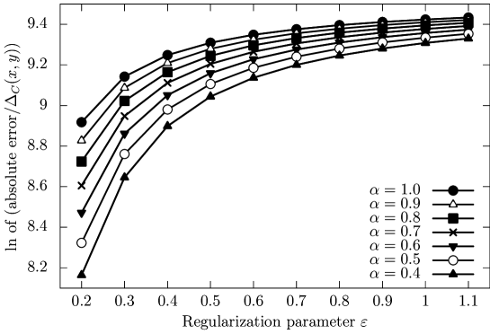
Figure 1. Absolute error$/\Delta_{C}(x,y)$ vs. regularization parameter $\varepsilon$.

7. Concluding remarks

In this paper, we considered regularization of optimal transport problems via Bregman divergence. We proved that the optimal value of the regularized problem converges to that of the given problem. More precisely, our error estimate becomes faster than exponentially. Numerical experiments showed that regularization by a Bregman divergence outperforms that by the Kullback–Leibler divergence.

There are several future directions subsequent to this study. The time complexity of our regularized problem is left open. It would also be interesting to extend the setting of this paper from a finite set to Euclidean space.

Acknowledgements

KM was supported in part by JSPS KAKENHI Grant Numbers JP20K14356,JP21H03451. KS was supported in part by JSPS KAKENHI Grant Numbers JP22K03425, JP22K18677, JP23H00086. AT was supported in part by JSPS KAKENHI Grant Numbers JP19K03494, JP19H01786. The authors are sincerely grateful to Maria Matveev and Shin-ichi Ohta for helpful discussion.