Drift Control of High-Dimensional RBM: A Computational Method Based on Neural Networks

Abstract

Motivated by applications in queueing theory, we consider a stochastic control problem whose state space is the $d$-dimensional positive orthant. The controlled process $Z$ evolves as a reflected Brownian motion whose covariance matrix is exogenously specified, as are its directions of reflection from the orthant’s boundary surfaces. A system manager chooses a drift vector $\theta(t)$ at each time $t$ based on the history of $Z$, and the cost rate at time $t$ depends on both $Z(t)$ and $\theta(t)$. In our initial problem formulation, the objective is to minimize expected discounted cost over an infinite planning horizon, after which we treat the corresponding ergodic control problem. Extending earlier work by Han et al. (Proceedings of the National Academy of Sciences, 2018, 8505-8510), we develop and illustrate a simulation-based computational method that relies heavily on deep neural network technology. For test problems studied thus far, our method is accurate to within a fraction of one percent, and is computationally feasible in dimensions up to at least $d=30$.

1 Introduction

Beginning with the seminal work of Iglehart and Whitt [26, 27], there has developed over the last 50+ years a large literature that justifies the use of reflected Brownian motions as approximate models of queueing systems under “heavy traffic” conditions. In particular, a limit theorem proved by Reiman [39] justifies the use of $d$-dimensional reflected Brownian motion (RBM) as an approximate model of a $d$-station queueing network. Reiman’s theory is restricted to networks of the generalized Jackson type, also called single-class networks, or networks with homogeneous customer populations, but it has been extended to more complex multi-class networks under certain restrictions, most notably by Peterson [37] and Williams [45]. The survey papers by Williams [44] and by Harrison and Nguyen [20] provide an overview of heavy traffic limit theory through its first 25 years.

Many authors have commented on the compactness and simplicity of RBM as a mathematical model, at least in comparison with the conventional discrete-flow models that it replaces. For example, in the preface to Kushner [32]’s book on heavy traffic analysis one finds the following passage:

“These approximating [Brownian] models have the basic structure of the original problem, but are significantly simpler. Much inessential detail is eliminated … They greatly simplify analysis, design, and optimization, [yielding] good approximations to problems that would otherwise be intractable …”

Of course, having adopted RBM as a system model, one still confronts the question of how to do performance analysis, and in that regard there has been an important recent advance: Blanchet et al. [10] have developed a simulation-based method to estimate steady-state performance measures for RBM in dimensions up to 200, and those estimates come with performance guarantees.

Descriptive performance analysis versus optimal control. Early work on heavy traffic approximations, including the papers cited above, focused on descriptive performance analysis under fixed operating policies. Harrison [18, 19] expanded the framework to include consideration of dynamic control, using informal arguments to justify Brownian approximations for queueing network models where a system manager can make sequencing, routing and/or input control decisions. Early papers in that vein by Harrison and Wein [22, 23] and by Wein [43] dealt with Brownian models simple enough that their associated control problems could be solved analytically. But for larger systems and/or more complex decisions, the Brownian control problem that approximates an original queueing control problem may only be solvable numerically. Such stochastic control problems may be of several different types, depending on context.

At one end of the spectrum are drift control problems, in which the controlling agent can effect changes in system state only at bounded finite rates. At the other end of the spectrum are impulse control problems, in which the controlling agent can effect instantaneous jumps in system state, usually with an associated fixed cost. In between are singular control problems, in which the agent can effect instantaneous state changes of any desired size, usually at a cost proportional to the size of the displacement; see for example, Karatzas [28]. In this paper we develop a computational method for the first of those three problem classes, and then illustrate its use on selected test problems. Our method is a variant of the one developed by Han et al. [17] for solution of semi-linear partial differential equations, and in its implementation we have re-used substantial amounts of the code provided by Han et al. [17] and Zhou et al. [49].

Literature Review. Two of the most relevant streams of literature are i) drift rate control problems, and ii) solving PDEs using deep learning. Ata et al. [5] considers a one-dimensional drift rate control problem on a bounded interval under a general cost of control but no state costs. The authors characterize the optimal policy in closed form; and they discuss the application of their model to a power control problem in wireless communication. Ormeci Matoglu and Vande Vate [36] consider a drift rate control problem where a system controller incurs a fixed cost to change the drift rate. The authors prove that a deterministic, non-overlapping control band policy is optimal; also see Vande Vate [42]. Ghosh and Weerasinghe [15, 16] extend Ata et al. [5] by incorporating state costs, abandonments and optimally choosing the interval where the process lives.

Drift control problems arise in a broad range of applications in practice. Rubino and Ata [40] studies a dynamic scheduling problem for a make-to-order manufacturing system. The authors model order cancellations as abandonments from their queueing system. This model feature gives rise to a drift rate control problem in the heavy traffic limit. Ata et al. [6] uses a drift control model to study a dynamic staffing problem in order to determine the number of volunteer gleaners, who sign up to help but may not show up, for harvesting leftover crops donated by farmers for the purpose of feeding food-insecure individuals. Bar-Ilan et al. [7] use a drift control model to study international reserves.

All of the papers mentioned above study one-dimensional drift-rate control problems. To the best of our knowledge, there have not been any papers studying such problems in high dimensions. One exception to this is the recent working paper Ata and Kasikaralar [4] that studies dynamic scheduling of a multiclass queue motivated by call center industry. Focusing on the Halfin-Whitt asymptotic regime, the authors derive a (limiting) drift rate control problem whose state space is $\mathbb{R}^{d}$, where $d$ is the number of buffers in their queueing model. Similar to us, the authors build on Han et al. [17] to solve their (high-dimensional) drift rate control problem. However, our work differs from theirs significantly, because their control problem has no state space constraints.

As mentioned earlier, our work builds on the seminal paper Han et al. [17]. In the last five years, there have been many papers written on solving PDEs using deep neural networks. We refer the reader to the recent survey Beck et al. [8]; also see E et al. [14].

The remainder of this paper. Section 2 recapitulates essential background knowledge from RBM theory, after which Section 3 states in precise mathematical terms the discounted control and ergodic control problems that are the object of our study. In each case, the problem statement is expressed in probabilistic terms initially, and then re-expressed analytically in the form of an equivalent Hamilton-Jacobi-Bellman equation (hereafter abbreviated to HJB equation). Section 4 derives key identities, that significantly contribute to the subsequent development of our computational method. Section 5 describes our computational method in detail.

Section 6 specifies three families of drift control test problems, each of which has members of dimensions $d=1,2,\ldots$ . The first two families arise as heavy traffic limits of certain queueing network control problems, and we explain that motivation in some detail. Drift control problems in the third family have a separable structure that allows them to be solved exactly by analytical means, which is of obvious value for assessing the accuracy of our computational method. Section 7 presents numerical results obtained with our method for all three families of test problems. In that admittedly limited context, our computed solutions are accurate to within a fraction of one percent, and our method remains computationally feasible up to at least dimension $d=30$, and in some cases up to dimension 100 or more. In Section 8 we describe variations and generalizations of the problems formulated in Section 3 that are of interest for various purposes, and which we expect to be addressed in future work. Finally, there are a number of appendices that contain proofs or other technical elaboration for arguments or procedures that have only been sketched in the body of the paper.

2 RBM preliminaries

We consider here a reflected Brownian motion $Z=\left\{Z(t),t\geq 0\right\}$ with state space $\mathbb{R}_{+}^{d},$ where $d\geq 1.$ The data of $Z$ are a (negative) drift vector $\mu\in\mathbb{R}^{d},$ a $d\times d$ positive-definite covariance matrix $A=(a_{ij}),$ and a $d\times d$ reflection matrix $R$ of the form

$$R=I-Q,\text{ where }Q\text{ has non-negative entries and spectral radius }\rho(Q)<1.$$ (1)

The restriction to reflection matrices of the form (1) is not essential for our purposes, but it simplifies the technical development and is consistent with usage in the related earlier paper by Blanchet et al. [10]. Denoting by $W=\left\{W(t),t\geq 0\right\}$ a $d$-dimensional Brownian motion with zero drift, covariance matrix $A$, and $W(0)=0$, we then have the representation

$$Z(t) =Z(0)+W(t)-\mu t+RY(t),\text{ }t\geq 0,\text{ where}$$ (2)

$$Y_{i}(\cdot) \text{ is continuous and non-decreasing with }Y_{i}(0)=0\text{ }(i=1,2,\ldots,d),\text{ and}$$ (3)

$$Y_{i}(\cdot) \text{ only increases at those times }t\text{ when }Z_{i}(t)=0\text{ }(i=1,2,\ldots,d).$$ (4)

Harrison and Reiman [21] showed that the relationships (1) to (4) determine $Y$ and $Z$ as pathwise functionals of $W,$ and that the mapping $W\rightarrow(Y,Z)$ is continuous in the topology of uniform convergence. We interpret the $i^{\text{th}}$ column of $R$ as the direction of reflection on the boundary surface $\{z\in\mathbb{R}_{+}^{d}:z_{i}=0\},$ and call $Y_{i}=\left\{Y_{i}(t),t\geq 0\right\}$ the “pushing process” on that boundary surface.

In preparation for future developments, let $f$   be an arbitrary $C^{2}$ (that is, twice continuously differentiable) function $\mathbb{R}^{d}\rightarrow\mathbb{R}$, and let $\nabla f$ denote its gradient vector as usual. Also, we define a second-order differential operator $\mathcal{L}$ via

$$\mathcal{L}f=\frac{1}{2}\sum_{i=1}^{d}\sum_{j=1}^{d}a_{ij}\frac{\partial^{2}}{\partial z_{i}\partial z_{j}}f,$$ (5)

and a first-order differential operator $\mathcal{D}=(\mathcal{D}_{1},\ldots,\mathcal{D}_{d})^{\top}$ via

$$\mathcal{D}f=R^{\top}\nabla f,$$ (6)

where $\top$ in (6) denotes transpose. Thus $\mathcal{D}_{i}f(\cdot)$ is the directional derivative of $f$ in the direction of reflection on the boundary surface $\left\{z_{i}=0\right\}.$ With these definitions, an application of Ito’s formula now gives the following identify, cf. Harrison and Reiman [21], Section 3:

$$\mathrm{d}f(X(t))=\nabla f(Z(t))\cdot\mathrm{d}W(t)+(\mathcal{L}f-\mu\cdot\nabla f)(Z(t))\,\mathrm{d}t+\mathcal{D}f(Z(t))\cdot\mathrm{d}Y(t),\ t\geq 0.$$ (7)

In the obvious way, the first inner product on the right side of (7) is shorthand for a sum of $d$ Ito differentials, while the last one is shorthand for a sum of $d$ Riemann-Stieltjes differentials.

3 Problem statements and HJB equations

Let us now consider a stochastic control problem whose state space is $\mathbb{R}_{+}^{d}$ $(d\geq 1).$ The controlled process $Z$ has the form

$$Z(t)=Z(0)+W(t)-\int_{0}^{t}\theta(s)\mathrm{d}s+RY(t),\ t\geq 0,$$ (8)

where (i) $W=\{W(t),t\geq 0\}$ is a $d$-dimensional Brownian motion with zero drift, covariance matrix $A$, and $W(0)=0$ as in Section 2, (ii) $\theta=\left\{\theta(t),t\geq 0\right\}$ is a non-anticipating control, or non-anticipating drift process, chosen by a system manager and taking values in a bounded set $\Theta\subset\mathbb{R}^{d},$ and (iii) $Y=\left\{Y(t),t\geq 0\right\}$ is a $d$-dimensional pushing process with components $Y_{i}$ that satisfy (3) and (4). Note that our sign convention on the drift in the basic system equation (8) is not standard. That is, we denote by $\theta(t)$ the negative drift vector at time $t$.

The control $\theta$ is chosen to optimize an economic objective (see below), and attention will be restricted to stationary Markov controls, or stationary control policies, by which we mean that

$$\theta(t)=u(Z(t)),\ t\geq 0\text{ for some measurable policy function }u:\mathbb{R}_{+}^{d}\rightarrow\Theta.$$ (9)

Hereafter the set $\Theta$ of drift vectors available to the system manager will be referred to as the action space for our control problem, a function $u:\mathbb{R}_{+}^{d}\rightarrow\Theta$ will simply be called a policy, and we denote by $Z^{u}$ the controlled RBM defined via (8) and (9). With regard to the system manager’s objective, we take as given a continuous cost function $c:\mathbb{R}_{+}^{d}\times\Theta\rightarrow\mathbb{R}$ with polynomial growth (see below for the precise meaning of that phrase), and assume that the cumulative cost incurred over the time interval $[0,t]$ under policy $u$ is

$$C^{u}(t)\equiv\int_{0}^{t}c(Z^{u}(s),u(Z^{u}(s)))\,\mathrm{d}s,\text{ }t\geq 0.$$ (10)

To be more specific, for $m,n\geq 1$, a function $g:D\subset\mathbb{R}^{m}\rightarrow\mathbb{R}^{n}$ is said to have polynomial growth if there exist constants $\alpha_{1},\,\beta_{1}>0$ such that

$$|g(z)|\leq\alpha_{1}\left(1+|z|^{\beta_{1}}\right),\ z\in D.$$

Because the action space $\Theta$ is bounded, the polynomial growth assumption on $c$ reduces to the following:

$$|c(z,\theta)|\leq\alpha_{2}\left(1+|z|^{\beta_{2}}\right)\text{ for all }z\in\mathbb{R}_{+}^{d}\text{ and }\theta\in\Theta,$$ (11)

where $\alpha_{2},\,\beta_{2}$ are positive constants.

Because our action space $\Theta$ is bounded by assumption, the controlled RBM $Z^{u}$ has bounded drift under any policy $u$, from which one can prove the following mild but useful property; see Appendix A for its proof.

Proposition 1.

Under any policy $u$ and for any integer $n=1,2,\ldots$ the function

$$g_{n}(z,t)=\mathbb{E}_{z}\left\{|Z^{u}(t)|^{n}\right\},\ t\geq 0,$$

has polynomial growth in $t$ for each fixed $z\in\mathbb{R}_{+}^{d}$.

3.1 Discounted control

In our first problem formulation, an interest rate $r>0$ is taken as given, and we adopt the following discounted cost objective: choose a policy $u$ to minimize

$$V^{u}(z)\equiv\mathbb{E}_{z}\left[\int_{0}^{\infty}e^{-rt}\mathrm{d}C^{u}(t)\right]=\mathbb{E}_{z}\left[\int_{0}^{\infty}e^{-rt}c(Z^{u}(t),u(Z^{u}(t)))\,\mathrm{d}t\right],$$ (12)

where $\mathbb{E}_{z}\left(\cdot\right)$ denotes a conditional expectation given that $Z(0)=z.$ Given the polynomial growth condition (11), it follows from Proposition 1 that the moments of $Z(t)$ are polynomially bounded as functions of $t$ for each fixed initial state $z$. Given the assumed positivity of the interest rate $r$, the expectation in (12) is therefore well defined and finite for each $z\in\mathbb{R}_{+}^{d}$.

Hereafter we refer to $V^{u}(\cdot)$ as the value function under policy $u$, and define the optimal value function

$$V(z)=\min_{u\in\,\mathcal{U}}V^{u}(z)\text{ for each }z\in\mathbb{R}_{+}^{d},$$ (13)

where $\mathcal{U}$ is the set of stationary Markov control policies. To solve for the value function $V^{u}(\cdot)$ under an arbitrary policy $u$, a standard argument gives the following PDE with boundary conditions, where $\mathcal{L}$ and $\mathcal{D}_{i}$ are the differential operators defined via (5) and (6), respectively:

$$\mathcal{L}V^{u}(z)-u(z)\cdot\nabla V^{u}(z)+c(z,u(z))=rV^{u}(z),\ \ z\in\mathbb{R}_{+}^{d},$$ (14)

with boundary conditions

$$\mathcal{D}_{i}V^{u}(z)=0\text{ if }z_{i}=0\text{ }(i=1,2,\ldots,d).$$ (15)

The corresponding HJB equation, to be solved for the optimal value function $V(\cdot),$ is

$$\mathcal{L}V(z)-\max_{\theta\in\Theta}\left\{\theta\cdot\nabla V(z)-c(z,\theta)\right\}=rV(z),z\in\mathbb{R}_{+}^{d},$$ (16)

with boundary conditions

$$\mathcal{D}_{i}V(z)=0\text{ if }z_{i}=0\text{ }(i=1,2,\ldots,d).$$ (17)

Moreover, the policy

$$u^{\ast}(z)=\arg\max_{\theta\in\Theta}\{\theta\cdot\nabla V(z)-c(z,\theta)\}$$ (18)

is optimal, meaning that $V^{u^{\ast}}(z)=V(z)$ for $z\in\mathbb{R}_{+}^{d}$.

There will be no attempt here to prove existence of $C^{2}$ solutions, but our computational method proceeds as if that were the case, striving to compute a $C^{2}$ function $V$ that satisfies (16)-(17) as closely as possible in a certain sense. In Appendix B.1 we use (7) to verify that a sufficiently regular solution of the PDE (14)-(15) does in fact satisfy (12) as intended, and similarly, that a sufficiently regular solution of (16)-(17) does in fact satisfy (13).

3.2 Ergodic control

For our second problem formulation, it is assumed that

$$c(z,\theta)\geq 0\text{ for all }(z,\theta)\in\mathbb{R}_{+}^{d}\times\Theta.$$ (19)

Readers will see that our analysis can be extended to cost functions that take on negative values in at least some states, but to do so one must deal with certain irritating technicalities. To be specific, the issue is whether the expected values involved in our formulation are well defined.

In preparation for future developments, let us recall that a square matrix $R$ of the form (1), called a Minkowski matrix in linear algebra (or just M-matrix for brevity), is non-singular, and its inverse is given by the Neumann expansion

$$R^{-1}=I+Q+Q^{2}+\ldots\geq 0.$$

Hereafter, we assume that

$$\text{there exists at least one }\theta\in\Theta\text{ such that }R^{-1}\theta>0.$$ (20)

It is known that an RBM with a non-singular covariance matrix, reflection matrix $R$, and negative drift vector $\theta$ has a stationary distribution if and only if the inequality in (20) holds, cf. Section 6 of Harrison and Williams [24]. Of course, our statement of this ”stability condition” reflects the non-standard sign convention used in this paper. That is, $\theta$ denotes the negative drift vector of the RBM under discussion.

For our ergodic control problem, a policy function $u:\mathbb{R}_{+}^{d}\rightarrow\Theta$ is said to be admissible if, first, the corresponding controlled RBM $Z^{u}$ has a unique stationary distribution $\pi^{u}$, and if, moreover,

$$\int_{\mathbb{R}_{+}^{d}}|f(z)|\,\pi^{u}(dz)<\infty$$ (21)

for any function $f:\mathbb{R}_{+}^{d}\rightarrow\mathbb{R}$ with polynomial growth. Our assumption (20) ensures the existence of at least one admissible policy $u$, as follows. Let $\theta\in\Theta$ be a negative drift vector satisfying (20), and consider the constant policy $u(\cdot)\equiv\theta$. The corresponding controlled process $Z^{u}$ is then an RBM having a unique stationary distribution $\pi^{u}$, as noted above. It has been shown in Budhiraja and Lee [11] that the moment generating function of $\pi^{u}$ is finite in a neighborhood of the origin, from which it follows that $\pi^{u}$ has finite moments of all orders. Thus $\pi^{u}$ satisfies (21) for any function $f$ with polynomial growth, so $u$ is admissible.

Because our cost function $c(z,\theta)$ has polynomial growth and our action space $\Theta$ is bounded, the steady-state average cost

$$\xi^{u}\equiv\int_{\mathbb{R}_{+}^{d}}c(z,u(z))\,\pi^{u}(dz)$$ (22)

is well defined and finite under any admissible policy $u$. The objective in our ergodic control problem is to find an admissible policy $u$ for which $\xi^{u}$ is minimal.

To solve for the steady-state average cost $\xi^{u}$ and the corresponding relative value function, denoted by $v^{u}(\cdot)$, under an admissible policy $u$, a standard argument gives the following PDE:

$$\mathcal{L}v^{u}(z)-u(z)\cdot\nabla v^{u}(z)+c(z,\theta)=\xi^{u}\text{ for each }z\in\mathbb{R}_{+}^{d},$$ (23)

with boundary conditions

$$\mathcal{D}_{i}v^{u}(z)=0\text{ if }z_{i}=0\text{ }(i=1,2,\ldots,d).$$ (24)

The HJB equation for ergodic control is again of a standard form, involving a constant $\xi$ (interpreted as the minimum achievable steady-state average cost) and a relative value function $v:\mathbb{R}_{+}^{d}\rightarrow\mathbb{R}$. To be specific, the HJB equation is

$$\mathcal{L}v(z)-\max_{\theta\in\Theta}\left\{\theta\cdot\nabla v(z)-c(z,\theta)\right\}=\xi\text{ for each }z\in\mathbb{R}_{+}^{d},$$ (25)

with boundary conditions

$$\mathcal{D}_{i}v(z)=0\text{ if }z_{i}=0\text{ }(i=1,2,\ldots,d).$$ (26)

Paralleling the previous development for discounted control, we show the following in Appendix B.2: if a $C^{2}$ function $v$ and a constant $\xi$ jointly satisfy (25)-(26), then

$$\xi=\inf_{u\in\mathcal{U}}\xi^{u},$$ (27)

where $\mathcal{U}$ denotes the set of admissible controls for the ergodic cost formulation. Moreover, the policy

$$u^{\ast}(z)=\arg\max_{\theta\in\Theta}\left\{\theta\cdot\nabla v(z)-c(z,\theta)\right\},\ z\in\mathbb{R}_{+}^{d},$$ (28)

is optimal, meaning that $\xi^{u^{\ast}}=\xi.$ Again paralleling the previous development for discounted control, there is no attempt to prove that such a solution for (25)-(26) exists. In Appendix B.2 we use (7) to verify that a sufficiently regular solution of the PDE (23)-(24) does in fact satisfy (22) as intended, and similarly, that a sufficiently regular solution of (25)-(26) does in fact satisfy (27).

4 Equivalent SDEs

In this section we prove two key identities, Equations (31) and (40) below, that are closely patterned after results used by Han et al. [17] to justify their ”deep BSDE method” for solution of certain non-linear PDEs. That earlier work provided both inspiration and detailed guidance for our study, but we include these derivations to make the current account as nearly self-contained as possible. Sections 4.1 and 4.2 treat the discounted and ergodic cases, respectively.

Our method begins by specifying what we call a reference policy. This is a nominal or default policy, specified at the outset but possibly revised in light of computational experience, that we use to generate sample paths of the controlled RBM $Z$. Roughly speaking, one wants to choose the reference policy so that its paths tend to occupy parts of the state space thought to be most frequently visited by an optimal policy.

4.1 Discounted control

Our reference policy for the discounted case chooses a constant action $u(z)=\tilde{\theta}>0$ in every state $z\in\mathbb{R}_{+}^{d}$. (Again we stress that, given the non-standard sign convention embodied in (8) and (19), this means that $\tilde{Z}$ has a constant drift vector $-\tilde{\theta}$, with all components negative.) Thus the corresponding reference process $\tilde{Z}$ is a $d$-dimensional RBM which, in combination with its $d$-dimensional pushing process $\tilde{Y}$ and the $d$-dimensional Brownian motion $W$ defined in Section 2, satisfies

$$\tilde{Z}(t)=\tilde{Z}(0)+W(t)-\tilde{\theta}\,t+R\,\tilde{Y}(t),\leavevmode\nobreak\ t\geq 0,$$ (29)

plus the obvious analogs of Equations (3) and (4). For the key identity (31) below, let

$$F(z,x)=\tilde{\theta}\cdot x-\max_{\theta\in\Theta}\left\{\theta\cdot x-c(z,\theta)\right\}\text{ for }z\in\mathbb{R}_{+}^{d}\text{ and }x\in\mathbb{R}^{d}.$$ (30)

Proposition 2.

If $V\left(\cdot\right)$ satisfies the HJB equation (16) - (17), then it also satisfies the following identity almost surely for any $T>0$:

$$e^{-rT}V(\tilde{Z}(T))-V(\tilde{Z}(0))=\int_{0}^{T}e^{-rt}\nabla V(\tilde{Z}(t))\cdot\mathrm{d}W(t)-\int_{0}^{T}e^{-rt}F(\tilde{Z}(t),\nabla V(\tilde{Z}(t)))\mathrm{d}t.$$ (31)

Proof.

Applying Ito’s formula to $e^{-rt}V(\tilde{Z}(t))$ and using Equation (7) yield

$$e^{-rT}V(\tilde{Z}(T))-V(\tilde{Z}(0)) = \int_{0}^{T}e^{-rt}\nabla V(\tilde{Z}(t))\cdot\mathrm{d}W(t)+\int_{0}^{T}e^{-rt}\mathcal{D}V(\tilde{Z}(t))\cdot\mathrm{d}\tilde{Y}(t)$$

$$+\int_{0}^{T}e^{-rt}\left(\mathcal{L}V(\tilde{Z}(t))-\tilde{\theta}\cdot\nabla V(\tilde{Z}(t))-rV(\tilde{Z}(t))\right)\mathrm{d}t.$$

Using the HJB boundary condition (17), plus the complementarity condition (4) for $\tilde{Y}$ and $\tilde{Z}$, one has

$$\int_{0}^{T}e^{-rt}\mathcal{D}V(\tilde{Z}(t))\cdot\mathrm{d}\tilde{Y}(t)=0.$$

Furthermore, substituting $z=\tilde{Z}(t)$ in the HJB equation (16), multiplying both sides by $e^{-rt}$, rearranging the terms, and integrating over $[0,T]$ yields

$$\int_{0}^{T}e^{-rt}\left(\mathcal{L}V(\tilde{Z}(t))-rV(\tilde{Z}(t))\right)\mathrm{d}t=\int_{0}^{T}e^{-rt}\max_{\theta\in\Theta}\left(\theta\cdot\nabla V(\tilde{Z}(t))-c(\tilde{Z}(t),\theta)\right)\mathrm{d}t.$$ (33)

Substituting Equation (33) into Equation (4.1) gives Equation (31). ∎

Proposition 2 provides the motivation for the loss function that we strive to minimize in our computational method (see Section 5). Before developing that approach, we prove the following, which can be viewed as a converse of Proposition 2.

Proposition 3.

Suppose that $V:\mathbb{R}_{+}^{d}\rightarrow\mathbb{R}$ is a $C^{2}$ function, $G:\mathbb{R}_{+}^{d}\rightarrow\mathbb{R}^{d}$ is continuous, and $V,\,\nabla V$, and $G$ all have polynomial growth. Also assume that the following identity holds almost surely for some fixed $T>0$ and every $Z(0)=z\in\mathbb{R}_{+}^{d}$:

$$e^{-rT}V(\tilde{Z}(T))-V(\tilde{Z}(0))=\int_{0}^{T}e^{-rt}G(\tilde{Z}(t))\cdot\mathrm{d}W(t)-\int_{0}^{T}e^{-rt}F(\tilde{Z}(t),G(\tilde{Z}(t)))\,\mathrm{d}t.$$ (34)

Then $G(\cdot)=\nabla V(\cdot)$ and $V$ satisfies the HJB equation (16) - (17).

Remark 1.

The surprising conclusion that (34) implies $\nabla V(\cdot)=G(\cdot)$, without any a priori relationship between $G$ and $\nabla V$ being assumed, motivates the “double parametrization” method in Section 5.

Proof of Proposition 3.

Because $\tilde{Z}$ is a time-homogeneous Markov process, we can express (34) equivalently as follows for any $k=0,1,\ldots$ :

$$e^{-rT}V(\tilde{Z}((k+1)T)-V(\tilde{Z}(kT) =\int_{kT}^{(k+1)T}e^{-r(t-kT)}G(\tilde{Z}(t))\cdot dW(t)$$

$$-\int_{kT}^{(k+1)T}e^{-r(t-kT)}F(\tilde{Z}(t),G(\tilde{Z}(t)))\,dt.$$ (35)

Now multiply both sides of (35) by $e^{-rkT}$, then add the resulting relationships for $k=0,1,\ldots,n-1$ to arrive at the following:

$$e^{-rnT}V(\tilde{Z}(nT))=V(\tilde{Z}(0))+\int_{0}^{nT}e^{-rt}G(\tilde{Z}(t))\cdot dW(t)-\int_{0}^{nT}e^{-rt}F(\tilde{Z}(t),G(\tilde{Z}(t)))dt.$$ (36)

Because $G$ has polynomial growth, one can show that

$$\mathbb{E}_{z}\left[\int_{0}^{nT}e^{-2rt}G(\tilde{Z}(t))^{2}dz\right]<\infty$$

for all $n\geq 1$. Thus, when we take $\mathbb{E}_{z}$ of both sides of (36), the stochastic integral (that is, the second term) on the right side vanishes, and then rearranging terms gives the following:

$$V(z)=e^{-rnT}\mathbb{E}_{z}\left[V(\tilde{Z}(nT))\right]+\mathbb{E}_{z}\left[\int_{0}^{nT}e^{-rt}F(\tilde{Z}(t),G(\tilde{Z}(t)))\mathrm{d}t\right],$$

for arbitrary positive integer $n.$

By Proposition 1 and the polynomial growth condition of $V$, we have $e^{-rnT}\mathbb{E}_{z}[V(\tilde{Z}(nT))]\rightarrow 0$ as $n\rightarrow\infty$. Therefore,

$$V(z)=\lim_{n\rightarrow\infty}\mathbb{E}_{z}\left[\int_{0}^{nT}e^{-rt}F\left(\tilde{Z}(t),G(\tilde{Z}(t))\right)\mathrm{d}t\right]\text{ for }z\in\mathbb{R}_{+}^{d}.$$

Similarly, since $F$ and $G$ have polynomial growth, we conclude that

$$\mathbb{E}_{z}\left[\int_{0}^{\infty}e^{-rt}\left|F\left(\tilde{Z}(t),G(\tilde{Z}(t))\right)\right|\mathrm{d}t\right]<+\infty\text{ for }z\in\mathbb{R}_{+}^{d},\text{ and }$$

$$\int_{0}^{nT}e^{-rt}F\left(\tilde{Z}(t),G(\tilde{Z}(t))\right)\mathrm{d}t\leq\int_{0}^{\infty}e^{-rt}\left|F\left(\tilde{Z}(t),G(\tilde{Z}(t))\right)\right|\mathrm{d}t<+\infty\text{ for }z\in\mathbb{R}_{+}^{d}.$$

Thus, by dominated convergence, we have

$$V(z)=\mathbb{E}_{z}\left[\int_{0}^{\infty}e^{-rt}F\left(\tilde{Z}(t),G(\tilde{Z}(t))\right)\mathrm{d}t\right]\text{ for }z\in\mathbb{R}_{+}^{d}.$$ (37)

In other words, $V(z)$ can be viewed as the expected discounted cost associated with the RBM under the reference policy starting in state $\tilde{Z}(0)=z,$ where $F\left(\cdot,G(\cdot)\right)$ is the state-cost function. Therefore, it follows from Equations (14) - (15) with $u(z)=\tilde{\theta}$ and $c(z,u(z))=c(z,\tilde{\theta})=F(z,G(z))$ for $z\in\mathbb{R}_{+}^{d}$ that $V$ satisfies the following PDE:

$$\mathcal{L}V(z)-\tilde{\theta}\cdot\nabla V(z)+F\left(z,G(z)\right)=rV(z),\ z\in\mathbb{R}_{+}^{d},$$ (38)

with boundary conditions (15), and that it has polynomial growth.

Suppose that $G(\cdot)=\nabla V(\cdot)$ (which we will prove later). Substituting this into Equation (38) and using the definition of $F$, it follows that

$$\mathcal{L}V(z)-\max_{\theta\in\Theta}\left\{\theta\cdot\nabla V(z)-c(z,\theta)\right\}=rV(z),\ z\in\mathbb{R}_{+}^{d},$$

which along with the boundary condition (15) gives the desired result.

To complete the proof, it remains to show that $G(\cdot)=\nabla V(\cdot).$ By applying Ito’s formula to $e^{-rt}V(\tilde{Z}(t))$ and using Equations (3)-(4) and (17), we conclude that

$$e^{-rT}V(\tilde{Z}(T))-V(\tilde{Z}(0))= \int_{0}^{T}e^{-rt}\left(\mathcal{L}V(\tilde{Z}(t))-\tilde{\theta}\cdot\nabla V(\tilde{Z}(t))-rV(\tilde{Z}(t))\right)\mathrm{d}t$$

$$+\int_{0}^{T}e^{-rt}\nabla V(\tilde{Z}(t))\cdot\mathrm{d}W(t).$$

Then, using Equation (38), we rewrite the preceding equation as follows:

$$e^{-rT}V(\tilde{Z}(T))-V(\tilde{Z}(0))=\int_{0}^{T}e^{-rt}\nabla V(\tilde{Z}(t))\cdot\mathrm{d}W(t)-\int_{0}^{T}e^{-rt}F\left(\tilde{Z}(t),G(\tilde{Z}(t))\right)\mathrm{d}t.$$

Comparing this with Equation (34) yields

$$\int_{0}^{T}e^{-rt}\left(G(\tilde{Z}(t))-\nabla V(\tilde{Z}(t))\right)\cdot\mathrm{d}W(t)=0,$$

which yields the following:

$$\mathbb{E}_{z}\left[\left(\int_{0}^{T}e^{-rt}\left(G(\tilde{Z}(t))-\nabla V(\tilde{Z}(t))\right)\cdot\mathrm{d}W(t)\right)^{2}\right]=0.$$ (39)

Thus, provided that $e^{-rt}\left(G(\tilde{Z}(t))-\nabla V(\tilde{Z}(t))\right)$ is square integrable, Ito’s isometry [48, Lemma D.1] yields the following:

$$\mathbb{E}_{z}\left[\left(\int_{0}^{T}e^{-rt}\left(G(\tilde{Z}(t))-\nabla V(\tilde{Z}(t))\right)\cdot\mathrm{d}W(t)\right)^{2}\right]=\mathbb{E}_{z}\left[\int_{0}^{T}\left\|e^{-rt}\left(G(\tilde{Z}(t))-\nabla V(\tilde{Z}(t))\right)\right\|_{A}^{2}\mathrm{d}t\right]=0,$$

where $\|x\|_{A}:=x^{\top}Ax$. The square integrability of $e^{-rt}\left(G(\tilde{Z}(t))-\nabla V(\tilde{Z}(t))\right)$ follows because $G$ and $\nabla V$ have polynomial growth and the action space $\Theta$ is bounded. Because of $A$ is a positive definite matrix, we then have $\nabla V(\tilde{Z}(t))=G(\tilde{Z}(t))$ almost surely. By the continuity of $\nabla V\left(\cdot\right)$ and $G(\cdot),$ we conclude that $\nabla V(\cdot)=G(\cdot)$. ∎

4.2 Ergodic control

Again we use a reference policy with constant (negative) drift vector $\tilde{\theta}$, and now we assume that $R^{-1}\tilde{\theta}>0$, which ensures that the reference policy is admissible for our ergodic control formulation. For the following analogs of Propositions 2 and 3, let

$$f(z,x)=\tilde{\theta}\cdot x-\max_{\theta\in\Theta}\left\{\theta\cdot x-c(z,\theta)\right\}\textrm{ for }x\in\mathbb{R}^{d},\,z\in\mathbb{R}_{+}^{d}.$$

Proposition 4.

If $v\left(\cdot\right)$ and $\xi$ solve the HJB equation (25) - (26), then we have

$$v(\tilde{Z}(T))-v(\tilde{Z}(0))=\int_{0}^{T}\nabla v(\tilde{Z}(t))\cdot\mathrm{d}W(t)+T\xi-\int_{0}^{T}f(\tilde{Z}(t),\nabla v(\tilde{Z}(t)))\,\mathrm{d}t.$$ (40)

Proof.

Applying Ito’s formula to $v(z)$ yields

$$v(\tilde{Z}(T)) -v(\tilde{Z}(0))$$ (41)

$$=\int_{0}^{T}\nabla v(\tilde{Z}(t))\cdot\mathrm{d}W(t)+\int_{0}^{T}\mathcal{D}v(\tilde{Z}(t))\cdot\mathrm{d}\tilde{Y}(t)+\int_{0}^{T}\left(\mathcal{L}v(\tilde{Z}(t))-\tilde{\theta}\cdot\nabla v(\tilde{Z}(t))\right)\mathrm{d}t.$$

Recall the boundary condition of the HJB equation is $\mathcal{D}_{j}v(z)=0$ if $z_{j}=0$. Thus Equations (3)-(4) jointly imply

$$\int_{0}^{T}\mathcal{D}v(\tilde{Z}(t))\cdot\mathrm{d}\tilde{Y}(t)=0.$$

Then, substituting the HJB equation (25) into Equation (41) gives (40). ∎

Proposition 5.

Suppose that $v:\mathbb{R}_{+}^{d}\rightarrow\mathbb{R}$ is a $C^{2}$ function, $g:\mathbb{R}_{+}^{d}\rightarrow\mathbb{R}^{d}$ is continuous, and $v,\,\nabla v,\,g$ all have polynomial growth. Also assume that the following identity holds almost surely for some fixed $T>0$, a scalar $\xi$ and every $Z(0)=z\in\mathbb{R}_{+}^{d}$:

$$v(\tilde{Z}(T))-v(\tilde{Z}(0))=\int_{0}^{T}g(\tilde{Z}(t))\cdot\mathrm{d}W(t)+T\xi-\int_{0}^{T}f(\tilde{Z}(t),g(\tilde{Z}(t)))\,\mathrm{d}t.$$ (42)

Then, $g(\cdot)=\nabla v(\cdot)$ and $(v,\xi)$ satisfies the HJB equation (16) - (17).

Proof.

Let $\tilde{\pi}$ be the stationary distribution of the RBM $\tilde{Z}$ under the reference policy and $\tilde{Z}(\infty)$ be a random variable with the distribution $\tilde{\pi}$. Then, assuming the initial distribution of the RBM under the reference policy is $\tilde{\pi}$, i.e. $\tilde{Z}(0)\sim\tilde{\pi}$, its marginal distribution at time t is also $\tilde{\pi}$, i.e. $\tilde{Z}(t)\sim\tilde{\pi}$ for every $t\geq 0$.

Because $g$ has polynomial growth, one can show that the expectation of the stochastic integral (that is, the first term) on the right side of (42) vanishes. Then, by taking the expectation over $\tilde{Z}(0)\sim\tilde{\pi},$ Equation (42) implies

$$\mathbb{E}_{\tilde{\pi}}\left[v(\tilde{Z}(0))\right]=\mathbb{E}_{\tilde{\pi}}\left[v(\tilde{Z}(T))\right]+\mathbb{E}_{\tilde{\pi}}\left[\int_{0}^{T}f(\tilde{Z}(t),g(\tilde{Z}(t)))\mathrm{d}t\right]-T\xi.$$ (43)

By observing that $\mathbb{E}_{\tilde{\pi}}[v(\tilde{Z}(0))]=\mathbb{E}_{\tilde{\pi}}[v(\tilde{Z}(T))]$ and

$$\mathbb{E}_{\tilde{\pi}}\left[f(\tilde{Z}(t),g(\tilde{Z}(t)))\right] = \mathbb{E}\left[f(\tilde{Z}(\infty),g(\tilde{Z}(\infty)))\right]\text{ for }t\geq 0,$$

we conclude that $\xi=\mathbb{E}[f(\tilde{Z}(\infty),g(\tilde{Z}(\infty)))]$. In other words, $\xi$ can be viewed as the expected steady-state cost associated with the RBM under the reference policy, where $f\left(\cdot,g(\cdot)\right)$ is the state-cost function. Therefore, it follows (by assumption) from Equations (23) - (24) with $u(z)=\tilde{\theta}$ and $c(z,u(z))=c(z,\theta)=f(z,g(z))$ for $z\in\mathbb{R}^{d}_{+}$ that there exists a $C^{2}$ relative value function $\tilde{v}$ with polynomial growth that satisfies the following PDE:

$$\mathcal{L}\tilde{v}(z)-\tilde{\theta}\cdot\nabla\tilde{v}(z)+f\left(z,g(z)\right)=\xi,\ \ z\in\mathbb{R}_{+}^{d},$$ (44)

with boundary conditions $\mathcal{D}_{i}\tilde{v}(z)=0\text{ if }z_{i}=0\ \ (i=1,\ldots,d)$. Furthermore, applying Ito’s formula to $\tilde{v}(\tilde{Z}(t))$ yields

$$\tilde{v}(\tilde{Z}(T))- \tilde{v}(\tilde{Z}(0))$$ (45)

$$=\int_{0}^{T}\nabla\tilde{v}(\tilde{Z}(t))\cdot\mathrm{d}W(t)+\int_{0}^{T}\mathcal{D}\tilde{v}(\tilde{Z}(t))\cdot\mathrm{d}\tilde{Y}(t)+\int_{0}^{T}\left(\mathcal{L}\tilde{v}(\tilde{Z}(t))-\tilde{\theta}\cdot\nabla\tilde{v}(\tilde{Z}(t))\right)\mathrm{d}t.$$

Since $\tilde{v}(z)$ also satisfies the boundary conditions $\mathcal{D}_{i}\tilde{v}(z)=0\text{ if }z_{i}=0\ \ (i=1,\ldots,d)$, it follows from Equations (3)-(4) that

$$\int_{0}^{T}\mathcal{D}\tilde{v}(\tilde{Z}(t))\cdot\mathrm{d}\tilde{Y}(t)=0.$$

Then, substituting Equation (44) into Equation (45) gives

$$\tilde{v}(\tilde{Z}(T))-\tilde{v}(\tilde{Z}(0))=\int_{0}^{T}\nabla\tilde{v}(\tilde{Z}(t))\cdot\mathrm{d}W(t)+T\xi-\int_{0}^{T}f(\tilde{Z}(t),g(\tilde{Z}(t)))\,\mathrm{d}t.$$ (46)

In the proof of Proposition 3, we first showed that, because $\tilde{Z}$ is a time-homogeneous Markov process, the assumed stochastic relationship (34) can be extended to the more general form (36) with $n$ an arbitrary positive integer. In the current context one can argue in exactly the same way to establish the following. First, the assumed stochastic relationship (42) actually holds in the more general form where $T$ is replaced by $nT$, with $n$ an arbitrary positive integer. As a consequence, the derived stochastic relationship (46) also holds with $nT$ in place of $T$. And finally, after taking expectations on both sides of those generalized versions of (42) and (46) we arrive at the following:

$$v(z) = \mathbb{E}_{z}\left[v(\tilde{Z}(nT))\right]-nT\xi+\mathbb{E}_{z}\left[\int_{0}^{nT}f(\tilde{Z}(t),g(\tilde{Z}(t)))\mathrm{d}t\right],\text{ and}$$ (47)

$$\tilde{v}(z) = \mathbb{E}_{z}\left[\tilde{v}(\tilde{Z}(nT))\right]-nT\xi+\mathbb{E}_{z}\left[\int_{0}^{nT}f(\tilde{Z}(t),g(\tilde{Z}(t)))\mathrm{d}t\right],$$ (48)

for $z\in\mathbb{R}_{+}^{d}$ and an arbitrary positive integer $n.$ Note that the expectation of the stochastic integral vanishes because $\nabla\tilde{v}$ has polynomial growth. Subtracting (48) from (47) further yields

$$v(z)-\tilde{v}(z)=\mathbb{E}_{z}\left[v(Z(nT))\right]-\mathbb{E}_{z}\left[\tilde{v}(Z(nT))\right].$$

Without loss of generality, we assume $\mathbb{E}\left[\tilde{v}(\tilde{Z}(\infty))\right]=\mathbb{E}\left[v(\tilde{Z}(\infty))\right]$. Since $v(\cdot)$ and $\tilde{v}(\cdot)$ have polynomial growth and the reference policy is admissible, we have that $\sup_{n>0}\mathbb{E}_{z}\left[(v(\tilde{Z}(nT)))^{2}\right]<\infty$ and $\sup_{n>0}\mathbb{E}_{z}\left[(\tilde{v}(\tilde{Z}(nT)))^{2}\right]<\infty$ by Equation (21). Then, by the Vitali convergence theorem, we have

$$\lim_{n\rightarrow+\infty}\mathbb{E}_{z}\left[v(Z(nT))\right] = \mathbb{E}\left[v(\tilde{Z}(\infty))\right]\text{ and}$$

$$\lim_{n\rightarrow+\infty}\mathbb{E}_{z}\left[\tilde{v}(Z(nT))\right] = \mathbb{E}\left[\tilde{v}(\tilde{Z}(\infty))\right].$$

Therefore, we have

$$v(z)-\tilde{v}(z)=\lim_{n\rightarrow+\infty}\left(\mathbb{E}_{z}\left[v(Z(nT))\right]-\mathbb{E}_{z}\left[\tilde{v}(Z(nT))\right]\right)=0\text{ for }z\in\mathbb{R}_{+}^{d},$$

which means $v(\cdot)$ also satisfies the PDE (44) and the associated boundary conditions. That is,

$$\mathcal{L}v(z)-\tilde{\theta}\cdot\nabla v(z)+f\left(z,g(z)\right)=\xi,\text{ for }z\in\mathbb{R}_{+}^{d}.$$ (49)

$$\mathcal{D}_{i}v(z)=0\text{ if }z_{i}=0\ \ (i=1,\ldots,d).$$ (50)

Suppose that $g(\cdot)=\nabla v(\cdot)$ (which we will prove later). Substituting this into Equation (49) and using the definition of $f$, it follows that

$$\mathcal{L}v(z)-\max_{\theta\in\Theta}\left\{\theta\cdot\nabla v(z)-c(z,\theta)\right\}=\xi,\ \ z\in\mathbb{R}_{+}^{d},$$

which along with the boundary condition (50) gives the desired result.

To complete the proof, it remains to show that $g(\cdot)=\nabla v(\cdot).$ By applying Ito’s formula to $v(\tilde{Z}(t))$ and using Equations (3)-(4) and (50), we conclude that

$$v(\tilde{Z}(T))-v(\tilde{Z}(0))=\int_{0}^{T}\left(\mathcal{L}v(\tilde{Z}(t))-\tilde{\theta}\cdot\nabla v(\tilde{Z}(t))\right)\mathrm{d}t+\int_{0}^{T}\nabla v(\tilde{Z}(t))\cdot\mathrm{d}W(t).$$

Then, using Equation (49), we rewrite the preceding equation as follows:

$$v(\tilde{Z}(T))-v(\tilde{Z}(0))=T\xi-\int_{0}^{T}f\left(\tilde{Z}(t),g(\tilde{Z}(t))\right)\mathrm{d}t+\int_{0}^{T}\nabla v(\tilde{Z}(t))\cdot\mathrm{d}W(t).$$

Comparing this with Equation (42) yields

$$\int_{0}^{T}\left(g(\tilde{Z}(t))-\nabla v(\tilde{Z}(t))\right)\cdot\mathrm{d}W(t)=0,$$

which yields the following:

$$\mathbb{E}_{z}\left[\left(\int_{0}^{T}\left(g(\tilde{Z}(t))-\nabla v(\tilde{Z}(t))\right)\cdot\mathrm{d}W(t)\right)^{2}\right]=0.$$ (51)

Thus, provided $g(\tilde{Z}(t))-\nabla v(\tilde{Z}(t))$ is square integrable, Ito’s isometry [48, Lemma D.1] gives the following:

$$\mathbb{E}_{z}\left[\left(\int_{0}^{T}\left(g(\tilde{Z}(t))-\nabla v(\tilde{Z}(t))\right)\cdot\mathrm{d}W(t)\right)^{2}\right]=\mathbb{E}_{z}\left[\int_{0}^{T}\left\|g(\tilde{Z}(t))-\nabla v(\tilde{Z}(t))\right\|_{A}^{2}\mathrm{d}t\right]=0.$$

The square integrability of $g(\tilde{Z}(t))-\nabla v(\tilde{Z}(t))$ follows because $g$ and $\nabla v$ have polynomial growth, and $\mathbb{E}_{z}\left(|\tilde{Z}(nT)|^{k}\right)$ is finite for all $k$ because our action space $\Theta$ is bounded. Then, since $A$ is positive definite, $\nabla v(\tilde{Z}(t))=g(\tilde{Z}(t))$ almost surely. By the continuity of $\nabla v\left(\cdot\right)$ and $g(\cdot),$ we conclude that $\nabla v(\cdot)=g(\cdot)$. ∎

5 Computational method

We follow in the footsteps of Han et al. [17], who developed a computational method to solve semilinear parabolic partial differential equations (PDEs). Those authors focused on a backward stochastic differential equation (BSDE) associated with their PDE, and in similar fashion, we focus on the stochastic differential equations (34) and (42) that are associated with our two stochastic control formulations (see Section 4). Our method differs from that of Han et al. [17], because they consider PDEs on a finite-time interval with an unbounded state space and a specified terminal condition, whereas our stochastic control problem has an infinite time horizon and state space constraints. As such, it leads to a PDE on a polyhedral domain with oblique derivative boundary conditions. We modify the approach of [17] to incorporate those additional features, treating the discounted and ergodic formulations in Sections 5.1 and 5.2, respectively.

5.1 Discounted control

We approximate the value function $V(\cdot)$ and its gradient $\nabla V(\cdot)$ by deep neural networks $V_{w_{1}}(\cdot)$ and $G_{w_{2}}(\cdot)$, respectively, with associated parameter vectors $w_{1}$ and $w_{2}$. Seeking an approximate solution of the stochastic equation (34), we define the loss function

$$\ell(w_{1},w_{2}) = \mathbb{E}\left[\left(e^{-rT}\,V_{w_{1}}(\tilde{Z}(T))-V_{w_{1}}(\tilde{Z}(0))\right.\right.$$

$$\left.\left.-\int_{0}^{T}e^{-rt}G_{w_{2}}(\tilde{Z}(t))\cdot\mathrm{d}W(t)+\int_{0}^{T}e^{-rt}F(\tilde{Z}(t),G_{w_{2}}(\tilde{Z}(t)))\,\mathrm{d}t\right)^{2}\right],$$

Here the expectation is taken with respect to the sample path distribution of our reference process $\tilde{Z}$, which will be specified in Algorithm 3 below. Our definition (5.1) of the loss function does not explicitly enforce the consistency requirement $\nabla V_{w_{1}}(\cdot)=G_{w_{2}}(\cdot)$, but Proposition 3 provides the justification for this separate parametrization. This type of double parametrization has also been implemented by Zhou et al. [49].

Subroutine 1 Euler discretization scheme

1:The drift vector $-\tilde{\theta}$, the covariance matrix $A$, the reflection matrix $R$, the time horizon $T$, a step-size $h$ (for simplicity, we assume $N\triangleq T/h$ is an integer), and a starting point $\tilde{Z}(0)=z$.

2:A discretized reflected Brownian motion and the Brownian increments at times $h,2h,\ldots,Nh$.

3:function Discretize($T,h,z$)

4:     For time interval $[0,T]$ and $N=T/h$, construct the partition $0=t_{0}<t_{1}<\ldots<t_{N}=T$, where $\Delta t_{n}=t_{n+1}-t_{n}=h$ for $n=0,1,\ldots,N-1$.

5:     Generate $N$ i.i.d. $d$-dimensional Gaussian random variables with mean zero and covariance matrix $hA$, denoted by $\delta_{0},\ldots,\delta_{N-1}$.

6:     for $k\leftarrow 0$ to $N-1$  do

7:         $x\leftarrow\tilde{Z}(kh)+\delta_{k}-\tilde{\theta}h$

8:         $\tilde{Z}((k+1)h)\leftarrow$ Skorokhod($x$)

9:     end for

10:     return $\tilde{Z}(h),\tilde{Z}(2h),\ldots,\tilde{Z}(Nh)$ and $\delta_{0}$,…,$\delta_{N-1}$.

11:end function

Subroutine 2 Solve the Skorokhod problem (linear complementarity problem)

1:A vector $x\in\mathbb{R}^{d}$ and the reflection matrix $R$.

2:A solution to the Skorokhod problem $y\in\mathbb{R}^{d}_{+}$

3:Set $\epsilon=10^{-8}$;

4:function Skorokhod($x$)

5:     ${y}={x}$;

6:     while Exists ${y}_{i}<-\epsilon$ do

7:         Compute the set $B=\{i:{y}_{i}<\epsilon$};

8:         Compute ${L}_{B}=-R_{B,B}^{-1}{x}_{B}$;

9:         Compute ${y}={x}+R_{:,B}\times{L}_{B}$;

10:     end while

11:     return ${y}$.

12:end function

Our computational method seeks a neural network parameter combination $(w_{1},w_{2})$ that minimizes an approximation of the loss defined via (5.1). Specifically, we first simulate multiple discretized paths of the reference RBM $\tilde{Z}$, restricted to a fixed and finite time domain $[0,T]$. To do that, we sample discretized paths of the underlying Brownian motion $W$, and then solve a discretized Skorohod problem for each path of $W$ (this is the purpose of Subroutine 2) to obtain the corresponding path of $\tilde{Z}$. Thereafter, our method computes a discretized version of the loss (5.1), summing over sampled paths to approximate the expectation and over discrete time steps to approximate the integral over $[0,T]$, and minimizes it using stochastic gradient descent; see Algorithm 3. In Subroutine 2, given the index set $B$, $R_{B,B}$ is the submatrix derived by deleting the rows and columns of $R$ with indices in $\{1,\ldots,d\}$\$B$. Similarly, $R_{:,B}$ is the matrix that one arrives at by deleting the columns of $R$ whose indices are in the set $\{1,\ldots,d\}$\$B$.

Algorithm 3 Method for the discounted control case

1:The number of iteration steps $M$, a batch size $B$, a learning rate $\alpha$, a time horizon $T$, a discretization step-size $h$ (for simplicity, we assume $N\triangleq T/h$ is an integer), a starting point $z$, and an optimization solver (SGD, ADAM, RMSProp, etc).

2:A neural network approximation of the value function ${V}_{w_{1}}$ and the gradient function $G_{w_{2}}$.

3:Initialize the neural networks ${V}_{w_{1}}$ and $G_{w_{2}}$; set $z_{0}^{(i)}=z$ for $i=1,2,...,B$.

4:for $k\leftarrow 0$ to $M-1$  do

5:     Simulate $B$ discretized RBM paths and the Brownian increments $\{\tilde{Z}^{(i)},\delta^{(i)}\}$ with a time horizon $T$ and a discretization step-size $h$ starting from $\tilde{Z}^{(i)}(0)=z_{k}^{(i)}$ by invoking Discretize($T,h,z_{k}^{(i)}$) for $i=1,2,...,B$.

6:     Compute the empirical loss

$$\hat{\ell}(w_{1},w_{2}) = \frac{1}{B}\sum_{i=1}^{B}\left(e^{-rT}V_{w_{1}}(\tilde{Z}^{(i)}(T))-V_{w_{1}}(\tilde{Z}^{(i)}(0))\right.$$

$$\left.-\sum_{j=0}^{N-1}e^{-rhj}G_{w_{2}}(\tilde{Z}^{(i)}(hj))\cdot\delta_{j}^{(i)}+\sum_{j=0}^{N-1}e^{-rhj}F(\tilde{Z}^{(i)}(hj),G_{w_{2}}(\tilde{Z}^{(i)}(hj)))h\right)^{2}.$$

7:     Compute the gradient $\partial{\hat{\ell}(w_{1},w_{2})}/\partial w_{1},\partial{\hat{\ell}(w_{1},w_{2})}/\partial w_{2}$ and update $w_{1},w_{2}$ using the chosen optimization solver.

8:     Update $z_{k+1}^{(i)}$ as the end point of the path $\tilde{Z}^{(i)}$: $z_{k+1}^{(i)}\leftarrow\tilde{Z}^{(i)}(T)$.

9:end for

10:return Functions $V_{w_{1}}(\cdot)$ and $G_{w_{2}}(\cdot)$.

After the parameter values $w_{1}$ and $w_{2}$ have been determined, our proposed policy is as follows:

$$\theta_{w_{2}}(z)=\arg\max_{\theta\in\Theta}\left(\theta\cdot G_{w_{2}}(z)-c(z,\theta)\right),\ z\in\mathbb{R}_{+}^{d}.$$ (54)

Remark 2.

One can also consider the policy using $\nabla V_{w_{1}}(\cdot)$ instead of $G_{w_{2}}(\cdot).$ That is,

$$\arg\max_{\theta\in\Theta}\left(\theta\cdot\nabla V_{w_{1}}(z)-c(z,\theta)\right),\ z\in\mathbb{R}_{+}^{d}.$$ (55)

However, our numerical experiments suggest that this policy is inferior to (54).

5.2 Ergodic control

We parametrize $v(\cdot)$ and $\nabla v(\cdot)$ using deep neural networks $v_{w_{1}}(\cdot)$ and $g_{w_{2}}(\cdot)$ with parameters $w_{1}$ and $w_{2}$, respectively, and then use Equation (42) to define an auxiliary loss function

$$\tilde{\ell}(w_{1},w_{2},\xi) = \mathbb{E}\left[\left(v_{w_{1}}(\tilde{Z}(T))-v_{w_{1}}(\tilde{Z}(0))\right.\right.$$

$$\left.\left.-\int_{0}^{T}g_{w_{2}}(\tilde{Z}(t))\mathrm{d}W(t)-T\xi+\int_{0}^{T}f\left(\tilde{Z}(t),g_{w_{2}}\left(\tilde{Z}(t)\right)\right)\mathrm{d}t\right)^{2}\right].$$

Then, defining the loss function $\ell(w_{1},w_{2})=\min_{\xi}\ell(w_{1},w_{2},\xi)$ and noting that

$$\mathrm{Var}\left(X\right)=\min_{\xi}\mathbb{E[}\left(X-\xi\right)^{2}\mathbb{]},$$

we arrive at the following expression for the loss function

$$\ell(w_{1},w_{2})=\mathrm{Var}\left(v_{w_{1}}(\tilde{Z}(T))-v_{w_{1}}(\tilde{Z}(0))-\int_{0}^{T}g_{w_{2}}(\tilde{Z}(t))\mathrm{d}W(t)+\int_{0}^{T}f\left(\tilde{Z}(t),g_{w_{2}}\left(\tilde{Z}(t)\right)\right)\mathrm{d}t)\right).$$ (57)

We present our method for the ergodic control case formally in Algorithm 4.

Algorithm 4 Method for the ergodic control case

1:The number of iteration steps $M$, a batch size $B$, a learning rate $\alpha$, a time horizon $T$, a discretization step-size $h$ (for simplicity, we assume $N\triangleq T/h$ is an integer), a starting point $z$, and an optimization solver (SGD, ADAM, RMSProp, etc).

2:A neural network approximation of the value function ${v}_{w_{1}}$ and the gradient function $g_{w_{2}}$.

3:Initialize the neural networks ${v}_{w_{1}}$ and $g_{w_{2}}$; set $z_{0}^{(i)}=z$ for $i=1,2,...,B$.

4:for $k\leftarrow 0$ to $M-1$  do

5:     Simulate $B$ discretized RBM paths and the Brownian increments $\{\tilde{Z}^{(i)},\delta^{(i)}\}$ with a time horizon $T$ and a discretization step-size $h$ starting from $\tilde{Z}^{(i)}(0)=z_{k}^{(i)}$ by invoking Discretize($T,h,z_{k}^{(i)}$), for $i=1,2,...,B$.

6:     Compute the empirical loss

$$\hat{\ell}(w_{1},w_{2}) = \widehat{\mathrm{Var}}\left(v_{w_{1}}(\tilde{Z}^{(i)}(T))-v_{w_{1}}(\tilde{Z}^{(i)}(0))-\sum_{j=0}^{N-1}g_{w_{2}}(\tilde{Z}^{(i)}(hj))\cdot\delta^{(i)}_{j}\right.$$

$$\left.+\sum_{j=0}^{N-1}f\left(\tilde{Z}^{(i)}(hj),g_{w_{2}}\left(\tilde{Z}^{(i)}(hj)\right)\right)h\right).$$

7:     Compute the gradient $\partial{\hat{\ell}(w_{1},w_{2})}/\partial w_{1},\partial{\hat{\ell}(w_{1},w_{2})}/\partial w_{2}$ and update $w_{1},w_{2}$ using the chosen optimization solver.

8:     Update $z_{k+1}^{(i)}$ as the end point of the path $\tilde{Z}^{(i)}$: $z_{k+1}^{(i)}\leftarrow\tilde{Z}^{(i)}(T)$.

9:end for

10:return Functions $v_{w_{1}}(\cdot)$ and $g_{w_{2}}(\cdot)$.

After the parameters values $w_{1}$ and $w_{2}$ have been determined, our proposed policy is the following:

$$\bar{\theta}_{w_{2}}(z)=\arg\max_{\theta\in{\Theta}}\left(\theta\cdot g_{w_{2}}(z)-c(z,\theta)\right),\ z\in\mathbb{R}_{+}^{d}.$$

6 Three families of test problems

Here we specify three families of test problems for which numerical results will be presented later (see Section 7). Each family consists of RBM drift control problems indexed by $d=1,2,\ldots,$ where $d$ is the dimension of the orthant that serves as the problem’s state space. The first of the three problem families, specified in Section 6.1, is characterized by a feed-forward network structure and linear cost of control. Recapitulating earlier work by Ata [2], Section 6.2 explains the interpretation of such problems as “heavy traffic” limits of input control problems for certain feed-forward queueing networks.

Our second family of test problems is identical to the first one except that now the cost of control is quadratic rather than linear. The exact meaning of that phrase will be spelled out in Section 6.3, where we also explain the interpretation of such problems as heavy traffic limits of dynamic pricing problems for queueing networks. In Section 6.4, we describe two parametric families of policies with special structure that will be used later for comparison purposes in our numerical study. Finally, Section 6.5 specifies our third family of test problems, which have a separable structure that allows them to be solved exactly by analytical means. Such problems are of obvious value for evaluating the accuracy of our computational method.

6.1 Main example with linear cost of control

We consider a family of test problems with parameters $K=0,1,\ldots$, attaching to each such problem the index $d$ (mnemonic for dimension) $=K+1$. Problem $d$ has state space $\mathbb{R}_{+}^{d}$ and the $d\times d$ reflection matrix

$$R=\left[\begin{array}[]{cccc}1&&&\\ -p_{1}&1&&\\ \vdots&&\ddots&\\ -p_{K}&&&1\end{array}\right],$$ (59)

where $p_{1},\ldots,p_{K}>0$ and $p_{1}+\cdots+p_{K}=1$. Also, the set of drift vectors available in each state is

$$\Theta=\prod\limits_{k=0}^{K}\left[\underline{\theta}_{k},\overline{\theta}_{k}\right].$$ (60)

where the lower limit $\underline{\theta}_{k}$ and upper limit $\overline{\theta}_{k}$ are as specified in Section 6.2 below. Similarly, the $d\times d$ covariance matrix $A$ for problem $d$ is as specified in Section 6.2. Finally, the cost function for problem $d$ has the linear form

$$c(z,\theta)=h^{\top}z+c^{\top}\theta\ \text{ where }\ h,\,c\in\mathbb{R}_{+}^{d}.$$ (61)

That is, the cost rate $c(Z(t),u(Z(t)))$ that the system manager incurs under policy $u$ at time $t$ is linear in both the state vector $Z(t)$ and the chosen drift rate $u(Z(t))$.

In either the discounted control setting or the ergodic control setting, inspection of the HJB equation displayed earlier in Section 3 shows that, given this linear cost structure, there exists an optimal policy $u^{*}(\cdot)$ such that

$$\text{either }\ u_{k}^{*}(z)=\underline{\theta}_{k}\ \text{ or }\ u_{k}^{*}(z)=\overline{\theta}_{k}$$ (62)

for each state $z\ \in\mathbb{R}_{+}^{K+1}$ and each component $k=0,1,\ldots,K$.

In the next section we explain how drift control problems of the form specified here arise as heavy traffic limits in queueing theory. Strictly speaking, however, that interpretation of the test problems is inessential to the main subject of this paper: the computational results presented in Section 7 can be read without reference to the queueing theoretic interpretations of our test problems.

6.2 Interpretation as heavy traffic limits of queueing network control problems

Let us consider the feed-forward queueing network model of a make-to-order production system portrayed in Figure 1. There are $d=K+1$ buffers, represented by the open-ended rectangles, indexed by $k=0,1,\ldots,K.$ Each buffer has a dedicated server, represented by the circles in Figure 1. Arriving jobs wait in their designated buffer if the server is busy. There are two types of jobs arriving to the system: regular versus thin streams. Thin stream jobs have the same service time distributions as the regular jobs, but they differ from the regular jobs in two important ways: First, thin stream jobs can be turned away upon arrival. That is, a system manager can exercise admission control in this manner, but in contrast, she must admit all regular jobs arriving to the system. Second, the volume of thin stream jobs is smaller than that of the regular jobs; see Assumption 1.

Figure 1: A feedforward queueing newtork with thin arrival streams.

Regular jobs enter the systems only through buffer zero, as shown by the solid arrow pointing to buffer zero in Figure 1. A renewal process $E=\{E(t):t\geq 0\}$ models the cumulative number of regular jobs arriving to the system over time. We let $\lambda$ denote the arrival rate and $a^{2}$ denote the squared coefficient of variation of the interarrival times for the regular jobs. The thin stream jobs arrive to buffer $k$ (as shown by the dashed arrows in Figure 1) according to the renewal process $A_{k}=\{A_{k}(t):t\geq 0\}$ for $k=0,1,\ldots,K$. We let $\eta_{k}$ denote the arrival rate and $b_{k}^{2}$ denote the squared coefficient of variation of the interarrival times for renewal process $A_{k}$.

Jobs in buffer $k$ have i.i.d. general service time distributions with mean $m_{k}$ and squared coefficient of variation $s_{k}^{2}\geq 0,\ k=0,1,\ldots,K$; $\mu_{k}=1/m_{k}$ is the corresponding service rate. We let $S_{k}=\{S_{k}(t):t\geq 0\}$ denote the renewal process associated with the service completions by server $k$ for $k=1,\ldots,K$. To be specific, $S_{k}(t)$ denotes the number of jobs server $k$ processes by time $t$ if it incurs no idleness during $[0,t]$. The jobs in each buffer are served on a first-come-first-served (FCFS) basis, and servers work continuously unless their buffer is empty. After receiving service, jobs in buffer zero join buffer $k$ with probability $p_{k},\ k=1,2,\ldots,K$, independently of other events. This probabilistic routing structure is captured by a vector-valued process $\Phi(\cdot)$ where $\Phi_{k}(\ell)$ denotes the total number of jobs routed to buffer $k$ among the first $\ell$ jobs served by server zero for $k=1,\ldots,K$ and $\ell\geq 1$. We let $p=(p_{k})$ denote the $K$-dimensional vector of routing probabilities. Jobs in buffers $1,\ldots,K$ leave the system upon receiving service.

As stated earlier, the system manager makes admission control decisions for thin stream jobs. Turning away a thin stream job arriving to buffer $k$ (externally) results in a penalty of $c_{k}$. For mathematical convenience, we model admission control decisions as if the system manager can simply “turn off” each of the thin stream arrival processes as desired. In particular, we let $\Delta_{k}(t)$ denote the cumulative amount of time that the (external) thin stream input to buffer $k$ is turned off during the interval $[0,t]$. Thus, the vector-valued process $\Delta=(\Delta_{k})$ represents the admission control policy. Similarly, we let $T_{k}(t)$ denote the cumulative amount of time server $k$ is busy during the time interval $[0,t]$, and $I_{k}(t)=t-T_{k}(t)$ denotes the cumulative amount of idleness that server $K$ incurs during $[0,t]$.

Letting $Q_{k}(t)$ denote the number of jobs in buffer $k$ at time $t$, the vector-valued process $Q=(Q_{k})$ will be called the queue-length process. Given a control $\Delta=(\Delta_{k})$, assuming $Q(0)=0$, it follows that

$$Q_{0}(t) = E(t)+A_{0}(t-\Delta_{0}(t))-S_{0}(T_{0}(t))\geq 0,\text{ }\ t\geq 0,$$ (63)

$$Q_{k}(t) = A_{k}(t-\Delta_{k}(t))+\Phi_{k}\left(S_{0}(T_{0}(t))\right)-S_{k}(T_{k}(t))\geq 0,\text{ }\ t\geq 0,\text{ }\ k=1,\ldots,K.$$ (64)

Moreover, the following must hold:

$$I(\cdot)\text{ is continuous and nondecreasing with }I(0)=0,$$ (65)

$$I_{k}(\cdot)\text{ only increases at those times $t$ when }Q_{k}(t)=0,\ \ k=0,1,\ldots,K,$$ (66)

$$\Delta_{k}(t)-\Delta_{k}(s)\leq t-s,\ \ 0\leq s\leq t<\infty,\ \ k=0,1,\ldots,K.$$ (67)

$$I,\Delta\text{ are non-anticipating.}$$ (68)

The system manager also incurs a holding cost at rate $h_{k}$ per job in buffer $k$ per unit of time. We use the processes $\xi=\left\{\xi(t),t\geq 0\right\}$ as a proxy for the cumulative cost under a given admission control policy $\Delta\left(\cdot\right),$ where

$$\xi(t)=\sum_{k=0}^{K}c_{k}\eta_{k}\Delta_{k}(t)+\sum_{k=0}^{K}\int_{0}^{t}h_{k}Q_{k}(s)\,\mathrm{d}s,\ \ t\geq 0.$$

This is an approximation of the realized cost because the first term on the right-hand side replaces the admission control penalties actually incurred with their means.

In order to derive the approximating Brownian control problem, we consider a sequence of systems indexed by a system parameter $n=1,2,\ldots;$ we attach a superscript of $n$ to various quantities of interest. Following the approach used by Ata [2], we assume that the sequence of systems satisfies the following heavy traffic assumption.

Assumption 1.

For $n\geq 1,$ we have that

$$\lambda^{n}=n\lambda,\eta_{k}^{n}=\eta_{k}\sqrt{n}\text{ and }\mu_{k}^{n}=n\mu_{k}+\sqrt{n}\beta_{k},\ \ k=0,1,\ldots,K,$$

where $\lambda,$ $\mu_{k},\eta_{k}$ and $\beta_{k}$ are nonnegative constants. Moreover, we assume that

$$\lambda=\mu_{0}=\frac{\mu_{k}}{p_{k}}\ \text{ for }\ k=1,\ldots,K.$$

One starts the approximation procedure by defining suitably centered and scaled processes. For $n\geq 1,$ we define

$$\hat{E}^{n}(t) =\frac{E^{n}(t)-\lambda^{n}t}{\sqrt{n}}\quad \quad\hat{\Phi}^{n}(q)=\frac{\Phi\left([nq]\right)-p([nq])}{\sqrt{n}},\text{ }\ t\geq 0,\text{ }\ q\geq 0,$$ and

$$\hat{A}_{k}^{n} =\frac{Q^{n}(t)}{\sqrt{n}} \quad\hat{S}_{k}^{n}(t)=\frac{\text{ }S_{k}^{n}(t)-\mu_{k}^{n}t}{\sqrt{n}},\ t\geq 0,\ k=0,1,\ldots,K,$$ and

$$\hat{Q}^{n}(t) =\frac{Q^{n}(t)}{\sqrt{n}} \quad\hat{\xi}^{n}(t)=\frac{\xi^{n}(t)}{\sqrt{n}},\ t\geq 0.$$ and

In what follows, we assume

$$T_{k}^{n}(t)=t-\frac{1}{\sqrt{n}}I_{k}(t)+o\left(\frac{1}{\sqrt{n}}\right),\ t\geq 0,\ k=0,1,\ldots,K,$$ (69)

where $I_{k}(\cdot)$ is the limiting idleness process for server $k$; see [18] for an intuitive justification of (69).

Then, defining

$$\chi_{0}^{n}(t) = \hat{E}^{n}(t)+\hat{A}_{0}^{n}(t-\Delta_{0}(t))+\hat{S}_{0}^{n}(T_{0}^{n}(t)),\text{ }t\geq 0,$$

$$\chi_{k}^{n}(t) = \hat{A}_{k}^{n}(t-\Delta_{0}(t))+\Phi_{k}\left(\frac{1}{n}\hat{S}_{0}^{n}(T_{0}^{n}(t))\right)+p_{k}\hat{S}_{0}^{n}(T_{0}^{n}(t))$$

$$\quad-\hat{S}_{k}^{n}(T_{k}^{n}(t)),\text{ }t\geq 0,\text{ }k=1,2,\ldots,K,$$

and using Equations (63) - (64) and (69), it is straightforward to derive the following for $t\geq 0$ and $k=1,\ldots,K:$

$$\hat{Q}_{0}^{n}(t) = \chi_{0}^{n}(t)+\left(\eta_{0}-\beta_{0}\right)t-\eta_{0}\Delta_{0}(t)+\mu_{0}I_{0}(t)+o(1),$$ (70)

$$\hat{Q}_{k}^{n}(t) = \chi_{k}^{n}(t)+\left(\eta_{k}+p_{k}\beta_{0}-\beta_{k}\right)t-\eta_{k}\Delta_{k}(t)+\mu_{k}I_{k}(t)-p_{k}\mu_{0}I_{0}(t)+o(1).$$ (71)

Moreover, it follows from Equation (67) that $\Delta_{k}(t)$ is absolutely continuous. We denote its density by $\delta_{k}(\cdot),i.e.,$

$$\Delta_{k}(t)=\int_{0}^{t}\delta_{k}(s)\mathrm{d}s,\ t\geq 0,\text{ }k=0,1,\ldots,K,$$

where $\delta_{k}(t)\in[0,1].$ Using this, we write

$$\hat{\xi}^{n}(t)=\sum_{k=0}^{K}\int_{0}^{t}v_{k}\eta_{k}\delta_{k}(s)\mathrm{d}s+\sum_{k=0}^{K}\int_{0}^{t}h_{k}\hat{Q}_{k}^{n}(s)\mathrm{d}s,t\geq 0.$$ (72)

Then passing to the limit formally as $n\rightarrow\infty,$ and denoting the weak limit of $(\hat{Q}^{n},\hat{X}^{n},\hat{\xi}^{n})$ by $\left(Z,\chi,\xi\right),$ where $\chi$ is a $(K+1)$-dimensional driftless Brownian motion with covariance matrix (see Appendix C for its derivation)

$$A=\mu_{0}\left[\begin{array}[]{ccccc}s_{0}^{2}+a^{2}&-p_{1}s_{0}^{2}&\cdots&\cdots&-p_{K}s_{0}^{2}\\ -p_{1}s_{0}^{2}&p_{1}(1-p_{1})+p_{1}^{2}s_{0}^{2}+p_{1}s_{1}^{2}&p_{1}p_{2}\left(s_{0}^{2}-1\right)&\cdots&p_{1}p_{K}\left(s_{0}^{2}-1\right)\\ \vdots&p_{1}p_{2}\left(s_{0}^{2}-1\right)&\ddots&&\vdots\\ \vdots&\vdots&&\ddots&p_{K-1}p_{K}\left(s_{0}^{2}-1\right)\\ -p_{K}s_{0}^{2}&p_{1}p_{K}\left(s_{0}^{2}-1\right)&\cdots&\cdots&p_{K}(1-p_{K})+p_{K}^{2}s_{0}^{2}+p_{K}s_{K}^{2}\end{array}\right],$$

we deduce from (70) - (71) and (72) that

$$Z_{0}(t) = \chi_{0}(t)+(\eta_{0}-\beta_{0})t-\int_{0}^{t}\eta_{0}\delta_{0}(s)\mathrm{d}s+\mu_{0}I_{0}(t),$$

$$Z_{k}(t) = \chi_{k}(t)+\left(\eta_{k}+p_{k}\beta_{0}-\beta_{k}\right)t-\int_{0}^{t}\eta_{k}\delta_{k}(s)\mathrm{d}s+\mu_{k}I_{k}(t),k=1,\ldots,K,$$

$$\xi(t) = \sum_{k=0}^{K}\int_{0}^{t}v_{k}\eta_{k}\delta_{k}(s)\mathrm{d}s+\sum_{k=0}^{K}\int_{0}^{t}h_{k}Z_{k}(s)\mathrm{d}s.$$

In order to streamline the notation, we make the following change of variables:

$$Y_{k}(t) = \mu_{k}I_{k}(t),\text{ }k=0,\ldots,K,$$

$$\theta_{0}(t) = \eta_{0}\delta_{0}(t)-(\eta_{0}-\beta_{0}),\text{ }t\geq 0,$$

$$\theta_{k}(t) = \eta_{k}\delta_{k}(t)-\left(\eta_{k}+p_{k}\beta_{0}-\beta_{k}\right)$$

and let

$$\underline{\theta}_{0} = \beta_{0}\ \text{ and }\ \overline{\theta}_{k}=\beta_{0}-\eta_{0},$$

$$\underline{\theta}_{k} = \beta_{k}-p_{k}\beta_{0}\ \text{ and }\ \overline{\theta}_{k}=\beta_{k}-\eta_{k}-p_{k}\beta_{0},\ k=1,\ldots,K.$$

Lastly, we define the set of negative drift vectors available to the system manager as in Equation (60). As a result, we arrive at the following Brownian system model:

$$Z_{0}(t) = \chi_{0}(t)-\int_{0}^{t}\theta_{0}(s)\mathrm{d}s+Y_{0}(t),\ \ t\geq 0,$$ (73)

$$Z_{k}(t) = \chi_{k}(t)-\int_{0}^{t}\theta_{k}(s)\mathrm{d}s-Y_{k}(t)+p_{k}Y_{0}(t),\ \ k=1,\ldots,K,$$ (74)

which can be written as in Equation (2) with $d=K+1,$ where the reflection matrix $R$ is given by Equation (59). Moreover, the processes $Y,Z$ inherit properties in Equation (63) - (73) from their pre-limit counterparts in the queueing model, cf. Equations (65) - (66).

To minimize technical complexity, we restrict attention to stationary Markov control policies as done in Section 3. That is, $\theta(t)=u(Z(t))$ for $t\geq 0$ for some policy function $u:\mathbb{R}_{+}^{d}\rightarrow\Theta.$ Then, defining $c=\left(c_{0},c_{1},\ldots,c_{K}\right)^{\top},\leavevmode\nobreak\ h=\left(h_{0},h_{1},\ldots,h_{K}\right)^{\top}$ and

$$c(z,\theta)=h^{\top}z+c^{\top}\theta,$$

as in Equation (61), the cumulative cost incurred over the time interval $[0,t]$ under policy $u$ can be written as in Equation (10). Note that $C^{u}(t)$ and $\xi(t)$ differ only by a term that is independent of the control. Given $C^{u}(t),$ one can formulate the discounted control problem as done in Section 3.1. Similarly, the ergodic control problem can be formulated as done in Section 3.2.

Interpreting the solution of the drift control problem in the context of the queueing network formulation. Because the instantaneous cost rate $c(z,\theta)$ is linear in the control, inspection of the HJB equation reveals that the optimal control is of bang-bang nature. That is, $\theta_{k}(t)\in\{\underline{\theta}_{k},\overline{\theta}_{k}\}$ for all $k,t$ as stated in Equation (62). This can be interpreted in the context of the queueing network displayed in Figure 1 as follows: For $k=0,1,\ldots,K$, whenever $\theta_{k}(t)=\overline{\theta}_{k}$, the system manager turns away the thin stream jobs arriving to buffer $k$ externally, i.e., she shuts off the renewal process $A_{k}(\cdot)$ at time $t$. Otherwise, she admits them to the system. Of course, the optimal policy is determined by the gradient $\nabla V(z)$ of the value function through the HJB equation, which we solve for using the method described in Section 5.

6.3 Related example with quadratic cost of control

Çelik and Maglaras [12] and Ata and Barjesteh [3] advance formulations where a system manager controls the arrival rate of customers to a queueing system by exercising dynamic pricing. One can follow a similar approach for the feed-forward queueing networks displayed in Figure 1 with suitable modifications, e.g., the dashed arrows also correspond to arrivals of regular jobs. This ultimately results in a problem of drift control for RBM with the cost of control

$$c(\theta,z)=\sum_{k=0}^{K}\alpha_{k}(\theta_{k}-\underline{\theta}_{k})^{2}+\sum_{k=0}^{K}h_{k}z_{k},$$ (75)

where $\underline{\theta}$ is the drift rate vector corresponding to a nominal price vector.

6.4 Two parametric families of benchmark policies

Recall the optimal policy can be characterized as

$$u^{\ast}(z)=\arg\max_{\theta\in\Theta}\left\{\theta\cdot\nabla V(z)-c(z,\theta)\right\},\ z\in\mathbb{R}_{+}^{d}.$$ (76)

The benchmark policy for the main test problem. In our main test problem (see Section 6.1), we have $c(z,\theta)=h^{\top}z+c^{\top}\theta$. Therefore, it follows from (76) that for $k=0,1,\dots,K$,

$$u_{k}^{\ast}(z)=\left\{\begin{array}[]{c}\overline{\theta}_{k}\\ \underline{\theta}_{k}\end{array}\right.\begin{array}[]{l}\text{ if }\left(\nabla V(z)\right)_{k}\geq c_{k},\\ \text{ otherwise.}\end{array}$$

Namely, the optimal policy is of bang-bang type. Therefore, we consider the following linear-boundary policies as our benchmark polices: For $k=0,1,\ldots,K$,

$$u_{k}^{\mathrm{lbp}}(z)=\left\{\begin{array}[]{c}\overline{\theta}_{k}\\ \underline{\theta}_{k}\end{array}\right.\begin{array}[]{l}\text{ if }\beta_{k}^{\top}z\geq c_{k},\\ \text{ otherwise,}\end{array}$$

where $\beta_{0},\beta_{1}\ldots,\beta_{K}\in\mathbb{R}^{K+1}$ are vectors of policy parameters to be tuned.

In our numerical study, we focus attention on the symmetric case where

$$h_{0}>h_{1}=\ldots=h_{K},$$

$$c_{0}=c_{1}=\ldots=c_{K},$$

$$p_{1}=\ldots=p_{K}=\frac{1}{K},$$

$$\underline{\theta}_{1}=\ldots=\underline{\theta}_{K},$$

$$\overline{\theta}_{1}=\ldots=\overline{\theta}_{K}.$$

Due to this symmetry, the downstream buffers look identical. As such, we restrict attention to parameter vectors of the following form:

$$\beta_{0} = \left(\phi_{1},\phi_{2},\ldots,\phi_{2}\right),\text{ and}$$

$$\beta_{i} = (\phi_{3},\phi_{4},\ldots\phi_{4},\phi_{5},\phi_{4},\ldots,\phi_{4})\text{ where }\phi_{5}\text{ is the }i+1^{\text{st}}\text{ element of }\beta_{i}\text{ for }i=1,\ldots,K.$$

The parameter vector $\beta_{0}$, which is used to determine the benchmark policy for buffer zero, has two distinct parameters: $\phi_{1}$ and $\phi_{2}$. In considering the policy for buffer zero, $\phi_{1}$ captures the effect of its own queue length, whereas $\phi_{2}$ captures the effects of the downstream buffers $1,\ldots,K$. We use a common parameter for the downstream buffers because they look identical from the perspective of buffer zero. Similarly, the parameter vector $\beta_{i}\ (i=1,\ldots,K)$ has three distinct parameters: $\phi_{3},\,\phi_{4}$ and $\phi_{5}$, where $\phi_{3}$ is used as the multiplier for buffer zero (the upstream buffer), $\phi_{5}$ is used to capture the effect of buffer $i$ itself and $\phi_{4}$ is used for all other downstream buffers. Note that all $\beta_{i}$ use the same three parameters $\phi_{3},\,\phi_{4}$ and $\phi_{5}$ for $i=1,\ldots,K$. They only differ with respect to the position of $\phi_{5}$, i.e., it is in the $i+1^{\text{st}}$ position for $\beta_{i}$.

In summary, the benchmark policy uses five distinct parameters in the symmetric case. This allows us to do a brute-force search via simulation on a five-dimensional grid regardless of the number of buffers.

The benchmark policy for the test problem with the quadratic cost of control. In this case, substituting Equation (75) into Equation (76) gives the following characterization of the optimal policy:

$$u_{k}^{\ast}(z)=\underline{\theta}_{k}+\frac{(\nabla V(z))_{k}}{2\alpha_{k}},\ k=0,1,\ldots,K.$$ (77)

Namely, the optimal policy is affine in the gradient. Therefore, we consider the following affine-rate policies as our benchmark polices: For $k=0,1,\ldots,K$,

$$u_{k}^{\mathrm{arp}}(z)=\underline{\theta}_{k}+\beta_{k}^{\top}z,$$

where $\beta_{0},\beta_{1}\ldots,\beta_{K}\in\mathbb{R}^{K+1}$ are vectors of policy parameters to be tuned. We truncate this at the upper bound $\overline{\theta}_{k}$ if needed.

We focus attention on the symmetric case for this problem formulation too. To be specific, we assume

$$h_{0}>h_{1}=\ldots=h_{K},$$

$$\alpha_{0}=\alpha_{1}=\ldots=\alpha_{K},$$

$$p_{1}=\ldots=p_{K}=\frac{1}{K},$$

$$\underline{\theta}_{1}=\ldots=\underline{\theta}_{K},$$

$$\overline{\theta}_{1}=\ldots=\overline{\theta}_{K}.$$

Due to this symmetry, the downstream buffers look identical. As such, we restrict attention to parameter vectors of the following form:

$$\beta_{0} = \left(\phi_{1},\phi_{2},\ldots,\phi_{2}\right),\text{ and}$$

$$\beta_{i} = (\phi_{3},\phi_{4},\ldots\phi_{4},\phi_{5},\phi_{4},\ldots,\phi_{4})\text{ where }\phi_{5}\text{ is the }i+1^{\text{st}}\text{element for }i=1,\ldots,K.$$

As done for the first benchmark policy above, this particular form of the parameter vectors can be justified using the symmetry as well.

6.5 Parallel-server test problems

In this section, we consider a problem whose solution can be derived analytically by considering a one-dimensional problem. To be specific, we consider the parallel-server network that consists of $K$ identical single-server queues as displayed in Figure 2. Clearly, this network can be decomposed into $K$ separate single-server queues, leading to K separate one-dimensional problem formulations, which can be solved analytically, see Appendix D for details. For this example we have that $R=I_{d\times d}$ and $A=I_{d\times d}$. In addition, we assume that the action space $\Theta$ and the cost function $c(z,\theta)$ are the same as above.

Figure 2: A decomposable parallel-server queueing network.

7 Computational results

For the test problems introduced in Section 6, we now compare the performance of policies derived using our method (see Section 5) with the best benchmark we could find. The results show that our method performs well, and it remains computationally feasible up to at least dimension $d=30$. We implement our method using three-layer or four-layer neural networks with the elu activation function [38] in Tensorflow 2 [1], and using code adapted from that of Han et al. [17] and Zhou et al. [50]; see Appendix E for further details of our implementation.

For our main test problem with linear cost of control (introduced previously in Section 6.1), and also for its variant with quadratic cost of control (Section 6.3), the following parameter values are assumed: $h_{0}=2$, $h_{k}=1.9$ for $k=1,\ldots,K$, $c_{k}=1$ for $k=0,\ldots,K$, and $p_{k}=1/K$ for $k=1,\ldots,K$. Also, the reflection matrix $R$ and the covariance matrix $A$ for those families of problems are as follows:

$$R=\left[\begin{array}[]{cccc}1&&&\\ -1/K&1&&\\ \vdots&&\ddots&\\ -1/K&&&1\end{array}\right]\text{ and }A=\left[\begin{array}[]{ccccc}1&0&\cdots&\cdots&0\\ 0&1&-\frac{1}{K^{2}}&\cdots&-\frac{1}{K^{2}}\\ \vdots&-\frac{1}{K^{2}}&\ddots&&\vdots\\ \vdots&\vdots&&\ddots&-\frac{1}{K^{2}}\\ 0&-\frac{1}{K^{2}}&\cdots&\cdots&1\end{array}\right].$$

However, as stated previously in Section 6.5, the reflection matrix and covariance matrix for our parallel-server test problems are $R=I_{d\times d}$ and $A=I_{d\times d}$. Problems in that third class have $K=d$ buffers indexed by $k=1,\ldots,K$, and we set $h_{1}=2$ and $h_{k}=1.9$ for $k=2,\ldots,K$.

7.1 Main test problem with linear cost of control

For our main test problem with linear cost of control (Section 6.1), we take

$$\underline{\theta}_{k}=0\text{ and }\overline{\theta}_{k}=b\in\{2,10\}\text{ for all }k.$$

Also, interest rates $r=0.1$ and $r=0.01$ will be considered in the discounted case.

To begin, let us consider the simple case where $K=0$ (that is, there are no downstream buffers in the queueing network interpretation of the problem) and hence $d=1$. In this case, one can solve the HJB equation analytically; see Appendix D for details. For the discounted formulation with $r=0.1$, Figure 3 compares the derivative of the value function computed using the analytical solution, shown in blue, with the neural network approximation for it that we computed using our method, shown in red. (The comparisons for $r=0.01$ and the ergodic control case are similar.)

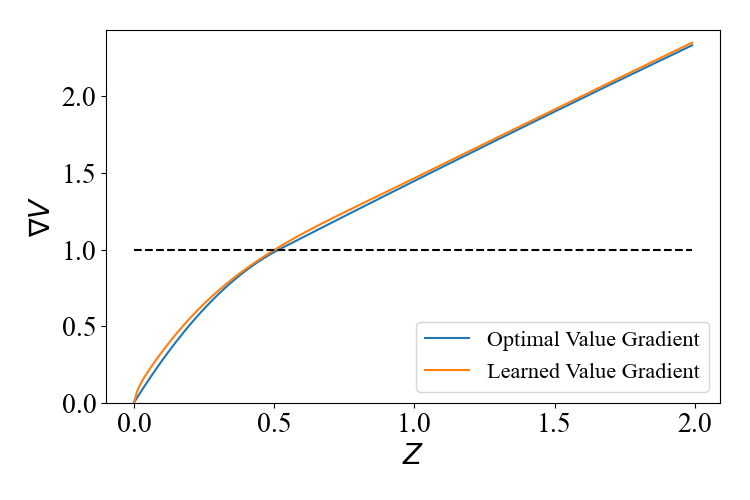
(a) $b=2$

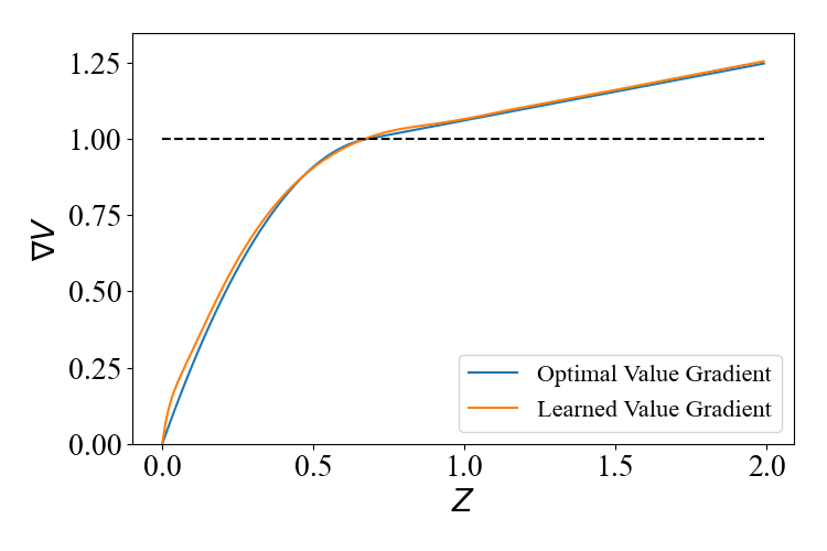
(b) $b=10$

Figure 3: Comparison between the derivative $G_{w}(\cdot)$ learned from neural networks and the derivative of the optimal value function for the case of $d=1$ and $r=0.1$. The dotted line indicates the cost $c_{0}=1$. When the value function gradient is above this dotted line, the optimal control is $\theta=b$, and otherwise it is $\theta=0$.

Combining Figure 3 with Equation (76), one sees that the policy derived using our method is close to the optimal policy. Table 1 reports the simulated performance with standard errors of these two policies based on four million sample paths and using the same discretization of time as in our computational method. Specifically, we report the long-run average cost under each policy in the ergodic control case, and report the simulated value $V(0)$ in the discounted case. To repeat, the benchmark policy in this case is the optimal policy determined analytically, but not accounting for the discretization of the time scale. Of course, all the performance figures reported in the table are subject to simulation errors. Finally, it is worth noting that our method took less than one hour to compute its policy recommendations using a 10-CPU core computer.

Table 1: Performance comparison of our proposed policy with the benchmark policy in the one-dimensional case ($K=0$).

		Ergodic	$r=0.01$	$r=0.1$
$b=2$	Our policy	1.455 $\pm$ 0.0006	145.3 $\pm$ 0.05	14.29 $\pm$ 0.004
	Benchmark	1.456 $\pm$ 0.0006	145.3 $\pm$ 0.05	14.29 $\pm$ 0.004
$b=10$	Our policy	1.375 $\pm$ 0.0007	137.2 $\pm$ 0.06	13.56 $\pm$ 0.005
	Benchmark	1.374 $\pm$ 0.0007	137.2 $\pm$ 0.06	13.56 $\pm$ 0.005

Table 2: Performance comparison of our proposed policy with the benchmark policy in the two-dimensional case ($K=1$).

		Ergodic	$r=0.01$	$r=0.1$
$b=2$	Our policy	2.471 $\pm$ 0.0008	246.6 $\pm$ 0.08	24.28 $\pm$ 0.006
	Benchmark	2.473 $\pm$ 0.0008	246.8 $\pm$ 0.08	24.29 $\pm$ 0.006
$b=10$	Our policy	2.338 $\pm$ 0.0009	233.3 $\pm$ 0.09	23.10 $\pm$ 0.006
	Benchmark	2.338 $\pm$ 0.0009	233.6 $\pm$ 0.09	23.10 $\pm$ 0.006

Let us consider now the two-dimensional case ($K=1$), where the optimal policy is unknown. Therefore, we compare our method with the best benchmark we could find: the linear boundary policy described in Section 6.4. In the two-dimensional case, the linear boundary policy reduces to the following:

$$\theta_{0}(z)=b\mathbb{I}\left\{\beta_{0}^{\top}z\geq 1\right\}\text{ and }\,\theta_{1}(z)=b\mathbb{I}\left\{\beta_{1}^{\top}z\geq 1\right\}.$$

Through simulation, we perform a brute-force search to identify the best values of $\beta_{0}$ and $\beta_{1}$. The policies for $b=2$ and $b=10$ are shown in Figures 4 and 5, respectively, for the discounted control case with $r=0.1$. Our proposed policy sets the drift to $b$ in the red region and to zero in the blue region, whereas the best-linear boundary policy is represented by the white-dotted line. That is, the benchmark policy sets the drift to $b$ in the region above and to the right of the dotted line, and sets it to zero below and left of the line. Table 2 presents the costs with standard errors of the benchmark policy and our proposed policy obtained in a simulation study. The two policies have similar performance. Our method takes about one hour to compute policy recommendations using a 10-CPU core computer.

(a) Server 0

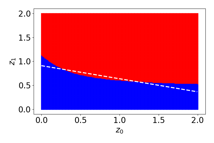
(b) Server 1

Figure 4: Graphical representation of the policy learned from neural networks and the benchmark policy for the case $b=2,d=2$ and $r=0.1$

(a) Server 0

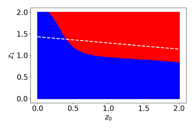
(b) Server 1

Figure 5: Graphical representation of the policy learned from neural networks and the benchmark policy for the case $b=10,d=2$ and $r=0.1$

Finally, let us consider the six-dimensional case ($K=5$), where the linear boundary policy reduces to

$$\theta_{i}(z)=b\mathbb{I}\left\{\beta_{i}^{\top}z\geq 1\right\}\text{ for }i=0,1,2,\ldots,5.$$

Although there appear to be 36 parameters to be tuned, recall that we reduced the number of parameters to five in Section 6.4 by exploiting symmetry. This makes the brute-force search computationally feasible. Table 3 compares the performance with standard errors of our proposed policies with the benchmark policies. They have similar performance. In this case, the running time for our method is several hours using a 10-CPU computer.

Table 3: Performance comparison of our proposed policy with the benchmark policy in the six-dimensional case $d=6$ ($K=5$).

		Ergodic	$r=0.01$	$r=0.1$
$b=2$	Our policy	7.927 $\pm$ 0.001	791.0 $\pm$ 0.1	77.83 $\pm$ 0.01
	Benchmark	7.927 $\pm$ 0.001	791.3 $\pm$ 0.1	77.83 $\pm$ 0.01
$b=10$	Our policy	7.565 $\pm$ 0.0016	754.8 $\pm$ 0.15	74.61 $\pm$ 0.01
	Benchmark	7.525 $\pm$ 0.0016	751.7 $\pm$ 0.15	74.32 $\pm$ 0.01

7.2 Test problems with quadratic cost of control

In this section, we consider the test problem introduced in Section 6.3, for which we set $\alpha_{k}=1$ and $\underline{\theta}_{k}=1$ for all $k$. As in the previous treatment of our main test example, we report results for the cases of $d=1,2,6$ in Tables 4, 5, 6, respectively, where the benchmark policies are the affine-rate policies discussed in Section 6.4, with policy parameters optimized via simulation and brute-force search. We observe that our proposed policies outperform the best affine-rate policies by very small margins in all cases.

Table 4: Performance comparison of our proposed policy with the benchmark policy in the case of quadratic cost of control and $d=1$.

	Ergodic	$r=0.01$	$r=0.1$
Our policy	0.757 $\pm$ 0.0004	75.53 $\pm$ 0.03	7.415 $\pm$ 0.003
Benchmark	0.758 $\pm$ 0.0004	75.67 $\pm$ 0.03	7.427 $\pm$ 0.003

Table 5: Performance comparison of our proposed policy with the benchmark policy in the case of quadratic cost of control and $d=2$ $(K=1)$

	Ergodic	$r=0.01$	$r=0.1$
Our policy	1.216 $\pm$ 0.0005	121.3 $\pm$ 0.04	11.94 $\pm$ 0.003
Benchmark	1.219 $\pm$ 0.0005	121.7 $\pm$ 0.05	11.96 $\pm$ 0.003

Table 6: Performance comparison of our proposed policy with the benchmark policy in the case of quadratic cost of control and $d=6$ $(K=5)$

	Ergodic	$r=0.01$	$r=0.1$
Our policy	3.863 $\pm$ 0.0008	385.7 $\pm$ 0.08	37.92 $\pm$ 0.006
Benchmark	3.874 $\pm$ 0.0008	386.9 $\pm$ 0.08	38.04 $\pm$ 0.006

In the one-dimensional ergodic control case ($K=0$), we obtain analytical solutions to the RBM control problem in closed form by solving the HJB equation directly, which reduces to a first-order ordinary differential equation in this case; see Appendix D for details. Figure 6 compares the derivative of the optimal value function (derived in closed form) with its approximation via neural networks in the ergodic case. Combining Figure 6 with Equation (77) reveals that our proposed policy is close to the optimal policy.

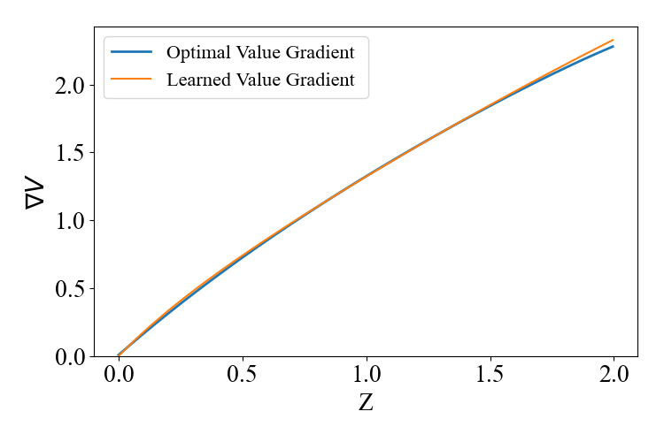
Figure 6: Comparison of the gradient approximation $G_{w}(\cdot)$ learned from neural networks with the derivative of the optimal value function for the ergodic control case with quadratic cost of control in the one-dimensional case ($d=1$).

In the two-dimensional case, our proposed policy is shown in Figure 7 for the ergodic case, with contour lines showing the state vectors ($z_{0},z_{1}$) for which the policy chooses successively higher drift rates. The white dotted lines similarly show the states ($z_{0},z_{1}$) for which our benchmark policy (that is, the best affine-rate policy) chooses the drift rate $\theta_{k}=1.5$ (for $k=0$ in the left panel and $k=1$ in the right panel).

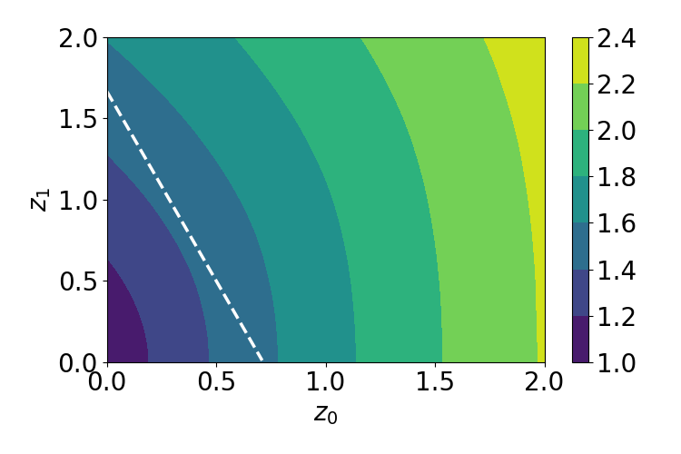
(a) Server 0

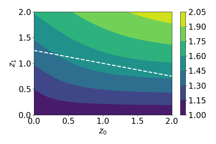
(b) Server 1

Figure 7: Graphical representation of the policy learned from neural networks and the benchmark policy for the ergodic case with $d=2$.

7.3 Parallel-server test problems

This section focuses on parallel-server test problems (see Section 6.5) to demonstrate our method’s scalability. As illustrated in Figure 2, the parallel-server networks are essentially $K$ independent copies of the one-dimensional case. We present the results in Table 7 for $d=30$ and linear cost of control. When $b=2$, our policies perform almost equally well as the optimal policy, while for $b=10$, our policies perform within 1% of the optimal policy. The run-time for our method is about one day in this case using a 20-CPU core computer.

Table 7: Performance comparison between our proposed policy and the benchmark policy for $30$-dimensional parallel-server test problems with linear cost of control.

		Ergodic	r = 0.01	r = 0.1
$b=2$	Our policy	42.56 $\pm$ 0.003	4247 $\pm$ 0.3	417.3 $\pm$ 0.02
	Benchmark	42.52 $\pm$ 0.003	4244 $\pm$ 0.3	417.2 $\pm$ 0.02
$b=10$	Our policy	40.53 $\pm$ 0.004	4054 $\pm$ 0.4	399.4 $\pm$ 0.026
	Benchmark	40.23 $\pm$ 0.004	4018 $\pm$ 0.4	396.7 $\pm$ 0.024

For quadratic cost of control, we are able to solve the test problems up to at least 100 dimensions. The results for $d=100$ are given in Table 8, where the benchmark policies are the best affine-rate policies (see Section 6.4). The performance of our policy is within 1% of the benchmark performance. The run-time for our method is several days in this case using a 30-CPU core computer.

Table 8: Performance comparison between our proposed policy and the benchmark policy for 100-dimensional parallel-server test problems with quadratic cost of control.

	Ergodic	$r=0.01$	$r=0.1$
Our policy	72.74 $\pm$ 0.003	7258.3 $\pm$ 0.3	712.4 $\pm$ 0.02
Benchmark	72.53 $\pm$ 0.003	7237.3 $\pm$ 0.3	710.2 $\pm$ 0.02

8 Concluding remarks

Consider the general drift control problem formulated in Section 3, assuming specifically that the instantaneous cost rate $c(z,\theta)$ is linear in $\theta$, and further assuming that the set of available drift vectors is a rectangle $\Theta=[0,b_{1}]\times\cdots\times[0,b_{d}]$. If one relaxes such a problem by letting $b_{i}\uparrow\infty$ for one or more $i$, then one obtains what is called a singular control problem, cf. Kushner and Martins [31]. Optimal policies for such problems typically involve the imposition of endogenous reflecting barriers, that is, reflecting barriers imposed by the system controller in order to minimize cost, in addition to exogenous reflecting barriers that may be imposed to represent physical constraints in the motivating application.

There are many examples of queueing network control problems whose natural heavy traffic approximations involve singular control; see, for example, Krichagina and Taksar [30], Martins and Kushner [34], and Martins et al. [33]. Given that motivation, we intend to show in future work how the computational method developed in this paper for drift control can be extended in a natural way to treat singular control, and to illustrate that extension by means of queueing network applications.

Separately, the following are three desirable generalizations of the problem formulations propounded in Section 3 of this paper. Each of them is straightforward in principle, and we expect to see these extensions implemented in future work, perhaps in combination with mild additional restrictions on problem data. (a) Instead of requiring that the reflection matrix $R$ have the Minkowski form (1), require only that $R$ be a completely-$\mathcal{S}$ matrix, which Taylor and Williams [41] showed is a necessary and sufficient condition for an RBM to be well defined. (b) Allow a more general state space for the controlled process $Z$, such as the convex polyhedrons characterized by Dai and Williams [13]. (c) Remove the requirement that the action space $\Theta$ be bounded.

Appendix A Proof of Proposition 1

Proof.

Let $f:\mathbb{R}_{+}\rightarrow\mathbb{R}^{d}$ be right continuous with left limits (rcll). Following Williams [46], we define the oscillation of $f$ over an interval $[t_{1},t_{2}]$ as follows:

$$Osc(f,[t_{1},t_{2}])=\sup\left\{|f(t)-f(s)|:t_{1}\leq s<t\leq t_{2}\right\},$$ (78)

where $|a|=\max_{i=1.\ldots,d}|a_{i}|$ for any $a\in\mathbb{R}^{d}$. Then for two rcll functions $f,g$, the following holds:

$$Osc(f+g)\leq Osc(f)+Osc(g).$$ (79)

Also recall that the controlled RBM $Z$ satisfies $Z(t)=X(t)+RY(t)$, where

$$X(t)=W(t)-\int_{0}^{t}\theta(s)ds,\ t\geq 0.$$ (80)

Then it follows from Theorem 5.1 of Williams [46] that

$$Osc(Z,[0,t]) \leq C\,Osc(X,[0,t])$$

$$\leq C\,Osc(W,[0,t])+C\bar{\theta}t$$

for some $C>0$, where $\bar{\theta}=\sum_{l=1}^{d}\left(\bar{\theta}_{l}-\underline{\theta}_{l}\right)$ and $\underline{\theta}_{l},\bar{\theta}_{l}$ are the minimal and maximal values on each dimension, and the second inequality follows from (79).

Let $\mathcal{O}=Ocs(W,[0,t])$ and recall that we are interested in bounding the expectation $\mathbb{E}\left[|Z(t)|^{n}\right]$. To that end, note that

$$\left|Z(t)-Z(0)\right|^{n} \leq C^{n}\left(\mathcal{O}+\bar{\theta}t\right)^{n}$$ (81)

$$= C^{n}\,\sum_{k=0}^{n}\binom{n}{k}\mathcal{O}^{k}\bar{\theta}^{n-k}t^{n-k}.$$

To bound $\mathbb{E}\left[\mathcal{O}^{k}\right],$ note that

$$\mathcal{O} \mathcal{=} \sup\left\{|W(t_{2})-W(t_{1})|:0\leq t_{1}<t_{2}\leq t\right\}$$

$$\leq \sup\left\{W(s):0\leq s\leq t\right\}-\inf\left\{W(s):0\leq s\leq t\right\}$$

$$\leq 2\sup\left\{|W(s)|:0\leq s\leq t\right\}$$

$$\leq 2\sup\left\{\sum_{l=1}^{d}|W_{l}(s)|:0\leq s\leq t\right\}$$

$$\leq 2\sum_{l=1}^{d}\sup\left\{|W_{l}(s)|:0\leq s\leq t\right\}.$$

So, by the union bound, we write

$$\mathbb{P}\left(\mathcal{O}>x\right) \leq \sum_{l=1}^{d}\mathbb{P}\left(\sup_{0\leq s\leq t}W_{l}(s)>\frac{x}{2d}\right)+\sum_{l=1}^{d}\mathbb{P}\left(\inf_{0\leq s\leq t}W_{l}(s)<-\frac{x}{2d}\right)$$

$$\leq 4\sum_{l=1}^{d}\mathbb{P}\left(W_{l}(t)>\frac{x}{2d}\right),$$

where the last inequality follows from the reflection principle.

Thus,

$$\mathbb{E}[\mathcal{O}^{k}]=\int_{0}^{\infty}x^{k-1}\mathbb{P}\left(\mathcal{O}>x\right)\mathrm{d}x\leq 4\sum_{l=1}^{d}\int_{0}^{\infty}x^{k-1}\mathbb{P}\left(W_{l}(t)>\frac{x}{2d}\right)\mathrm{d}x.$$

By change of variable $y=x/d,$ we write

$$\mathbb{E}[\mathcal{O}^{k}] \leq 4\sum_{l=1}^{d}\left(2d\right)^{k}\int_{0}^{\infty}y^{k-1}\mathbb{P}\left(W_{l}(t)>y\right)\mathrm{d}y$$

$$= 4\sum_{l=1}^{d}\left(2d\right)^{k}\mathbb{E}[|W_{l}(t)|^{k}]$$

$$= \frac{4\left(2d\right)^{k}2^{k/2}t^{k/2}\Gamma\left(\frac{k+1}{2}\right)}{\sqrt{\pi}}\sum_{l=1}^{d}\sigma_{ll}^{k},$$

where $\Gamma$ is the Gamma function, and the last equality is a well-known result; see, for example, Equation (12) in [47]. Substituting this into (81) gives the following:

$$\mathbb{E}[|Z(t)-Z(0)|^{n}] \leq C^{n}\sum_{k=0}^{n}\frac{4\left(2d\right)^{k}\binom{n}{k}2^{k/2}t^{k/2}\Gamma\left(\frac{k+1}{2}\right)}{\sqrt{\pi}}\bar{\theta}^{n-k}t^{n-k}\left(\sum_{l=1}^{d}\sigma_{ll}^{k}\right)$$ (82)

$$\leq \tilde{C}_{n}(t^{n}+1).$$

Letting $z=Z(0).$ We write

$$|Z(t)|^{n} = \left|Z(t)-z+z\right|^{n}\leq\left(|Z(t)-z|+|z|\right)^{n}$$

$$\leq \sum_{k=0}^{n}\binom{n}{k}\left|Z(t)-z\right|^{k}|z|^{n-k}.$$

Using (82), we can therefore write

$$\mathbb{E}\left[\left|Z(t)\right|^{n}\right] \leq \sum_{k=0}^{n}\binom{n}{k}\tilde{C}_{k}|z|^{n-k}\left(t^{k}+1\right)$$

$$\leq \hat{C}_{n}(1+t^{n}).$$

∎

Appendix B Validity of HJB Equations

B.1 Discounted Control

Proposition 6.

Let $u\in\mathcal{U}$ be an admissible policy and $V^{u}$ a $C^{2}$ solution of the associated PDE (14)-(15). If both $V^{u}$ and its gradient have polynomial growth, then $V^{u}$ satisfies (12).

Proof.

Applying Ito’s formula to $e^{-rt}\,V^{u}(Z^{u}(t))$ and using Equation (7), we write

$$e^{-rT}\,V^{u}(Z^{u}(T))-V^{u}(z)= \int_{0}^{T}e^{-rt}\,\left(\mathcal{L}V^{u}(Z^{u}(t))-u(Z^{u}(t))\cdot V^{u}(Z^{u}(t))-rV^{u}(Z^{u}(t))\right)dt$$

$$+\int_{0}^{T}e^{-rt}\mathcal{D}\,V^{u}(Z^{u}(t))\cdot dY(t)+\int_{0}^{T}e^{-rt}\,\nabla V^{u}(Z^{u}(t))\cdot dW(t).$$

Then using (3)-(4) and (14)-(15), we arrive at the following:

$$e^{-rT}\,V^{u}(Z^{u}(T))-V^{u}(z)=-\int_{0}^{T}e^{-rt}\,c(Z^{u}(t),u(Z^{u}(t)))\,dt+\int_{0}^{T}e^{-rt}\,\nabla V^{u}(Z^{u}(t))\cdot dW(t).$$ (83)

Because $\nabla V^{u}$ has polynomial growth and the action space $\Theta$ is bounded, we have that

$$\mathbb{E}_{z}\left[\int_{0}^{T}e^{-rt}\nabla\,V^{u}(Z^{u}(t))\cdot dW(t)\right]=0;$$

see, for example, Theorem 3.2.1 of Oksendal [35]. Thus, taking the expectation of both sides of (83) yields

$$V^{u}(z)=\mathbb{E}_{z}\left[\int_{0}^{T}e^{-rt}\,c(Z^{u}(t),u(Z^{u}(t)))\,dt\right]+e^{-rT}\,\mathbb{E}_{z}\left[V^{u}(Z^{u}(T))\right].$$

Because $V^{u}$ has polynomial growth and $\Theta$ is bounded, the second term on the right-hand side vanishes by as $T\rightarrow\infty$. Then, because $c$ has polynomial growth and $\Theta$ is bounded, passing to the limit as $T\rightarrow\infty$ completes the proof. ∎

Proposition 7.

If $V$ is a $C^{2}$ solution of the HJB equation (16)-(17), and if both $V$ and its gradient have polynomial growth, then $V$ satisfies (13).

Proof.

First, consider an arbitrary admissible policy $u$ and let $V^{u}$ denote the solution of the associated PDE (14)-(15). By Proposition 6, we have that

$$V^{u}(z)=\mathbb{E}_{z}\left[\int_{0}^{\infty}e^{-rt}\,c(Z^{u}(t),u(Z^{u}(t))\,dt\right],\ z\in\mathbb{R}_{+}^{d}.$$ (84)

On the other hand, because $V$ solves (16)-(17) and

$$u(z)\cdot\nabla V(z)-c(z,u(z))\leq\max_{\theta\in\Theta}\left\{\theta\cdot\nabla V(z)-c(z,\theta\right\},\ z\in\mathbb{R}_{+}^{d},$$

we conclude that

$$\mathcal{L}\,V(z)-u(z)\cdot\nabla V(z)+c(z,u(z))\geq r\,V(z).$$ (85)

Now applying Ito’s formula to $e^{-rt}\,V(Z^{u}(t))$ and using Equation (7) yields

$$e^{-rT}\,V(Z^{u}(T))-V(z)= \int_{0}^{T}\left(\mathcal{L}V(Z^{u}(t))-u(Z^{u}(t))\cdot\nabla V(Z^{u}(t))-rV(Z^{u}(t))\right)dt$$

$$+\int_{0}^{T}\mathcal{D}\,V(Z^{u}(t))\cdot dY(t)+\int_{0}^{T}e^{-rt}\nabla V(Z^{u}(t))\cdot dW(t).$$

Combining this with Equations (3)-(4), (16)-(17) and (85) gives

$$e^{-rT}\,V(Z^{u}(t))-V(z)\geq-\int_{0}^{T}e^{-rt}\,c(Z^{u}(t),u(Z^{u}(t)))\,dt+\int_{0}^{T}e^{-rt}\nabla V(Z^{u}(t))\cdot dW(t).$$ (86)

Because $\nabla V$ has polynomial growth and the action space $\Theta$ is bounded, we have that

$$\mathbb{E}_{z}\left[\int_{0}^{T}e^{-rt}\,\nabla V(Z^{u}(t))\cdot dW(t)\right]=0;$$

see, for example, Theorem 3.2.1 of Oksendal [35]. Using this and taking the expectation of both sides of Equation (86) yields

$$V(z)\leq\mathbb{E}_{z}\left[\int_{0}^{T}e^{-rt}\,c(Z^{u}(t),u(Z^{u}(t)))\,dt\right]+e^{-rT}\,\mathbb{E}\left[V(Z^{u}(T))\right].$$

Because $V$ has polynomial growth and $\Theta$ is bounded, the second term on the right-hand side vanishes as $T\rightarrow\infty$. Then, because $c$ has polynomial growth and $\Theta$ is bounded, passing to the limit yields

$$V(z)\leq\mathbb{E}_{z}\left[\int_{0}^{T}e^{-rt}\,c(Z^{u}(t),u(Z^{u}(t)))\,dt\right]=V^{u}(z),$$ (87)

where the equality holds by Equation (84).

Now, consider the optimal policy $u^{*}$, where $u^{*}(z)=\arg\max_{\theta\in\Theta}\left\{\theta\cdot\nabla V(z)-c(z,\theta)\right\}$. For notational brevity, let $Z^{*}=Z^{u^{*}}$ denote the RBM under policy $u^{*}$. Note from Equation (16) that

$$\mathcal{L}V(z)-u^{*}(z)\cdot\nabla V(z)+c(z,u^{*}(z))=rV(z),\ z\in\mathbb{R}_{+}^{d}.$$ (88)

Repeating the preceding steps with $u^{*}$ in place of $u$ and replacing the inequality with an equality, cf. Equations (85) and (88), we conclude that

$$V(z)=\mathbb{E}_{z}\left[\int_{0}^{\infty}e^{-rt}\,c(Z^{*}(t),u^{*}(Z^{*}(T)))\,dt\right]=V^{u^{*}}(z).$$

Combining this with Equation (87) yields (13). ∎

B.2 Ergodic Control

Proposition 8.

Let $u\in\mathcal{U}$ be an admissible policy and $(\tilde{\xi},v^{u})$ a $C^{2}$ solution of the associated PDE (23)-(24). Further assume that $v^{u}$ and its gradient have polynomial growth. Then

$$\tilde{\xi}=\xi^{u}=\int_{\mathbb{R}_{+}^{d}}c(z,u(z))\,\pi^{u}(dz).$$

Proof.

Let $\pi^{u}$ denote the stationary distribution of RBM under policy $u$, and let $Z^{u}$ denote the RBM under policy $u$ that is initiated with $\pi^{u}$. That is,

$$\mathbb{P}(Z^{u}(0)\in B)=\pi^{u}(B)\ \text{ for }B\subset\mathbb{R}_{+}^{d}.$$

Then applying Ito’s formula to $v^{u}(Z^{u}(t))$ and using Equation (7) yields

$$v^{u}(Z^{u}(t))-v^{u}(Z^{u}(0))= \int_{0}^{T}(\mathcal{L}v^{u}(Z^{u}(t))-u(Z^{u}(t))\cdot\nabla v^{u}(Z^{u}(t)))\,dt$$

$$+\int_{0}^{T}\mathcal{D}v^{u}(Z^{u}(t))\cdot dY(t)+\int_{0}^{T}\nabla v^{u}(Z^{u}(t))\cdot dW(t).$$

Then using Equations (3)-(4) and (23)-(24), we arrive at the following:

$$v^{u}(Z^{u}(T))-v^{u}(Z^{u}(0))=\int_{0}^{T}\left[\tilde{\xi}-c(Z^{u}(t),u(Z^{u}(t)))\right]dt+\int_{0}^{T}\nabla v^{u}(Z^{u}(t))\cdot dW(t).$$ (89)

Note that the marginal distribution of $Z^{u}(t)$ is $\pi^{u}$ for all $t\geq 0$. Thus, we have that

$$\mathbb{E}_{\pi^{u}}[v^{u}(Z^{u}(T))]=\mathbb{E}_{\pi^{u}}[v^{u}(Z^{u}(0))].$$

Moreover, using Equation (21) and the polynomial growth of $\nabla v^{u}$, we conclude that

$$\mathbb{E}_{\pi^{u}}\left[\int_{0}^{T}\left|\nabla v^{u}(Z^{u}(t))\right|^{2}\,dt\right]=T\,\int_{\mathbb{R}_{+}^{d}}\left|\nabla v^{u}(z)\right|^{2}\,\pi^{u}(dz)<\infty.$$

Consequently, we have that $\mathbb{E}\left[\int_{0}^{T}\nabla v^{u}(Z^{u}(t))\cdot dW(t)\right]=0$; see, for example, Theorem 3.2.1 of Oksendal [35]. Combining these and taking the expectation of both sides of (89) gives

$$\tilde{\xi}=\frac{1}{T}\int_{0}^{T}\mathbb{E}_{\pi^{u}}\left[c(Z^{u}(t),u(Z^{u}(t)))\right]\,dt=\int_{\mathbb{R}_{+}^{d}}c(z,u(z))\,\pi_{u}(dz)=\xi^{u}.$$

∎

Proposition 9.

Let $(v,\xi)$ be a $C^{2}$ solution of the HJB equation (25)-(26), and further assume that both $v$ and its gradient have polynomial growth. Then (27) holds, and moreover, $\xi=\xi^{u^{*}}$ where the optimal policy $u^{*}$ is defined by (28).

Proof.

First, consider an arbitrary policy $u$ and note that

$$\xi^{u}=\int_{\mathbb{R}_{+}^{d}}c(z,u(z))\,\pi^{u}(dz),$$

where $\pi^{u}$ is the stationary distribution of RBM under policy $u$. Let $Z^{u}$ denote the RBM under policy $u$ that is initiated with the stationary distribution $\pi^{u}$. That is,

$$\mathbb{P}(Z^{u}(0)\in B)=\pi^{u}(B),\ \ B\subset\mathbb{R}_{+}^{d}.$$

On the other hand, because ($v,\xi$) solves the HJB equation and

$$u(z)\cdot\nabla v(z)-c(z,u(z))\leq\max_{\theta\,\in\,\Theta}\left\{\theta\cdot\nabla v(z)-c(z,\theta)\right\},$$

we have that

$$\mathcal{L}v(z)-u(z)\cdot\nabla v(z)+c(z,u(z)))\geq\xi$$ (90)

Now, we apply Ito’s formula to $v(Z^{u}(t))$ and use Equation (7) to get

$$v(Z^{u}(T))-v(Z^{u}(0))= \int_{0}^{T}(\mathcal{L}v(Z^{u}(t)))-u(Z^{u}(t))\cdot\nabla v(Z^{u}(t))))\,dt$$

$$+\int_{0}^{T}\nabla v(Z^{u}(t))\cdot dY(t)+\int_{0}^{T}\nabla v(Z^{u}(t))\cdot dW(t).$$

Combining this with Equations (3)-(4), (26) and (90) gives

$$v(Z^{u}(T))-v(Z^{u}(0))\geq\int_{0}^{T}(\xi-c(Z^{u}(t),u(Z^{u}(t)))\,dt+\int_{0}^{T}\nabla v(Z^{u}(t))\cdot dW(t).$$ (91)

Note that the marginal distribution of $Z^{u}(t)$ is $\pi^{u}$ for all $t\geq 0$. Thus, we have that

$$\mathbb{E}_{\pi^{u}}[v(Z^{u}(T))]=\mathbb{E}_{\pi^{u}}[v(Z^{u}(0))].$$

Moreover, using Equation (21) and the polynomial growth of $\nabla v$, we conclude that

$$\mathbb{E}_{\pi^{u}}\left[\int_{0}^{T}\left|\nabla v(Z^{u}(t))\right|^{2}\,dt\right]=T\,\int_{\mathbb{R}_{+}^{d}}\left|\nabla v(z)\right|^{2}\,\pi^{u}(dz)<\infty.$$

Consequently, we have that $\mathbb{E}\left[\int_{0}^{T}\nabla v(Z^{u}(t))\,dW(t)\right]=0$; see for example Theorem 3.2.1 of Oksendal [35]. Combining these and taking the expectation of both sides of (91) give

$$\xi\,T\leq\int_{0}^{T}\mathbb{E}_{\pi^{u}}\left[c(Z^{u}(t),u(Z^{u}(t))\right]\,dt=T\,\mathbb{E}_{\pi^{u}}\left[c(Z^{u}(0),u(Z^{u}(0)))\right],$$

which yields

$$\xi\leq\mathbb{E}_{\pi^{u}}\left[c(Z^{u}(0),u(Z^{u}(0)))\right]=\int_{\mathbb{R}_{+}^{d}}c(z,u(z))\,\pi^{u}(dz)=\xi^{u}.$$ (92)

Now, consider policy $u^{*}$. For notational brevity, let $Z^{*}(t)=Z^{u^{*}}(t)$ denote the RBM under policy $u^{*}$ that is initiated with the stationary distribution $\pi^{u^{*}}$. In addition, note from (25) that

$$\mathcal{L}v(z)-u^{*}(z)\cdot\nabla v(z)+c(z,u^{*}(z))=\xi,\ \ z\in\mathbb{R}_{+}^{d}.$$ (93)

Repeating the preceding steps with $u^{*}$ in place of $u$ and replacing the inequality with an equality, cf. Equations (90) and (93), we conclude

$$\xi=\mathbb{E}_{\pi^{u^{*}}}\left[c(Z^{*}(0),u(Z^{*}(0)))\right]=\int_{\mathbb{R}_{+}^{d}}c(z,u^{*}(z))\,\pi^{u^{*}}(dz)=\xi^{u^{*}}.$$

Combining this with Equation (92) completes the proof. ∎

Appendix C Derivation of the covariance matrix of the feed-forward examples

By the functional central limit theorem for the renewal process [9], we have

$$\hat{E}^{n}(\cdot)\Rightarrow W_{E}\left(\cdot\right),$$

where $W_{E}\left(\cdot\right)$ is an one-dimensional Brownian motion with drift zero and variance $\lambda a^{2}=\mu_{0}a^{2}.$ Furthermore, we have

$$\hat{S}_{k}^{n}(t)\Rightarrow W_{k}\left(\cdot\right),\text{ for }k=1,2,\ldots,K,$$

where $W_{k}\left(\cdot\right)$ is an one-dimensional Brownian motion with drift zero and variance $\mu_{0}p_{k}s_{k}^{2}.$ Now, we turn to $\hat{S}_{0}^{n}(t)$ and $\hat{\Phi}^{n}(t).$ By Harrison [18], we have

$$\mathrm{Cov}\left(\left[\begin{array}[]{c}\hat{S}_{0}^{n}(t)\\ \hat{\Phi}^{n}(t)\end{array}\right]\right)=\mu_{0}\Omega^{0}+\mu_{0}s_{0}^{2}R^{0}\left(R^{0}\right)^{\top},$$

where $\Omega_{kl}^{0}=p_{k}(\mathbb{I}\{k=l\}-p_{l})$ for,$k,l=0,\ldots,K$ and $R^{0}=[1,-p_{1},\ldots,-p_{K}]^{\top}.$ Therefore, we have

$$\mathrm{Cov}\left(\left[\begin{array}[]{c}\hat{S}_{0}^{n}(t)\\ \hat{\Phi}^{n}(t)\end{array}\right]\right)=\mu_{0}\left[\begin{array}[]{ccccc}s_{0}^{2}&-p_{1}s_{0}^{2}&\cdots&\cdots&-p_{K}s_{0}^{2}\\ -p_{1}s_{0}^{2}&p_{1}(1-p_{1})+p_{1}^{2}s_{0}^{2}&p_{1}p_{2}\left(s_{0}^{2}-1\right)&\cdots&p_{1}p_{K}\left(s_{0}^{2}-1\right)\\ \vdots&p_{1}p_{2}\left(s_{0}^{2}-1\right)&\ddots&&\vdots\\ \vdots&\vdots&&\ddots&p_{K-1}p_{K}\left(s_{0}^{2}-1\right)\\ -p_{K}s_{0}^{2}&p_{1}p_{K}\left(s_{0}^{2}-1\right)&\cdots&\cdots&p_{K}(1-p_{K})+p_{K}^{2}s_{0}^{2}\end{array}\right].$$

Therefore, the variance of $\chi$ is

$$A = diag(\lambda a^{2},\mu_{1}s_{1}^{2},\ldots,\mu_{K}s_{K}^{2})+$$

$$\mu_{0}\left[\begin{array}[]{ccccc}s_{0}^{2}&-p_{1}s_{0}^{2}&\cdots&\cdots&-p_{K}s_{0}^{2}\\ -p_{1}s_{0}^{2}&p_{1}(1-p_{1})+p_{1}^{2}s_{0}^{2}&p_{1}p_{2}\left(s_{0}^{2}-1\right)&\cdots&p_{1}p_{K}\left(s_{0}^{2}-1\right)\\ \vdots&p_{1}p_{2}\left(s_{0}^{2}-1\right)&\ddots&&\vdots\\ \vdots&\vdots&&\ddots&p_{K-1}p_{K}\left(s_{0}^{2}-1\right)\\ -p_{K}s_{0}^{2}&p_{1}p_{K}\left(s_{0}^{2}-1\right)&\cdots&\cdots&p_{K}(1-p_{K})+p_{K}^{2}s_{0}^{2}\end{array}\right]$$

$$= \mu_{0}\left[\begin{array}[]{ccccc}s_{0}^{2}+a^{2}&-p_{1}s_{0}^{2}&\cdots&\cdots&-p_{K}s_{0}^{2}\\ -p_{1}s_{0}^{2}&p_{1}(1-p_{1})+p_{1}^{2}s_{0}^{2}+p_{1}s_{1}^{2}&p_{1}p_{2}\left(s_{0}^{2}-1\right)&\cdots&p_{1}p_{K}\left(s_{0}^{2}-1\right)\\ \vdots&p_{1}p_{2}\left(s_{0}^{2}-1\right)&\ddots&&\vdots\\ \vdots&\vdots&&\ddots&p_{K-1}p_{K}\left(s_{0}^{2}-1\right)\\ -p_{K}s_{0}^{2}&p_{1}p_{K}\left(s_{0}^{2}-1\right)&\cdots&\cdots&p_{K}(1-p_{K})+p_{K}^{2}s_{0}^{2}+p_{K}s_{K}^{2}\end{array}\right].$$

In particular, if the arrival and service processes are Poisson processes, we have $a=1$ and $s_{k}=1$ for $k=0,1,2,\ldots,K.$ Then, we have

$$A_{\mathrm{Poisson}}=\mu_{0}\left[\begin{array}[]{ccccc}2&-p_{1}&\cdots&\cdots&-p_{K}\\ -p_{1}&2p_{1}&&&\\ \vdots&&\ddots&&\\ \vdots&&&\ddots&\\ -p_{K}&&&&2p_{K}\end{array}\right]$$

Furthermore, if the service time for server zero is deterministic, i.e., $s_{0}=0$ , we have

$$A_{\mathrm{deterministic}}=\mu_{0}\left[\begin{array}[]{ccccc}a^{2}&0&\cdots&\cdots&0\\ 0&p_{1}(1-p_{1})+p_{1}s_{1}^{2}&-p_{1}p_{2}&\cdots&-p_{1}p_{K}\\ \vdots&-p_{1}p_{2}&\ddots&&\vdots\\ \vdots&\vdots&&\ddots&-p_{K-1}p_{K}\\ 0&-p_{1}p_{K}&\cdots&\cdots&p_{K}(1-p_{K})+p_{K}s_{K}^{2}\end{array}\right]$$

Appendix D ​​​ Analytical solution of one-dimensional test problems

D.1 Ergodic control formulation with linear cost of control

We consider the one-dimensional control problem with the cost function

$$c(z,\theta)=hz+c\theta\text{ for }z\in\mathbb{R}_{+}\text{ and }\theta\in\Theta=[0,b].$$

In the ergodic control case, the HJB equation (25) - (26) is

$$\frac{a}{2}v^{\prime\prime}(z)-\max_{\theta\in[0,b]}\left\{\theta\cdot v^{\prime}(z)-hz-c\theta\right\}=\xi,\text{ and}$$ (96)

$$v^{\prime}(0)=0\text{ and }v^{\prime}(z)\text{ having polynomial growth rate,}$$ (97)

where the covariance matrix $A=a$ in this one-dimensional case. The HJB equation (96) - (97) is equivalent to

$$\frac{a}{2}v^{\prime\prime}(z)+hz-(v^{\prime}(z)-c)^{+}b=\xi,$$

and the solution is

$$\left(v^{\ast}\right)^{\prime}(z)=\left\{\begin{array}[]{c}\frac{2}{\sqrt{a}}\sqrt{ch+\frac{ah^{2}}{4b^{2}}}z-\frac{h}{a}z^{2}\\ \frac{h}{b}z+\frac{ha}{2b^{2}}-\frac{\sqrt{a}}{b}\sqrt{ch+\frac{ah^{2}}{4b^{2}}}+c\text{ }\end{array}\right.\begin{array}[]{c}\text{if }z<z^{\ast}\\ \text{if }z\geq z^{\ast}\end{array},\text{ with}$$

$$z^{*}=\frac{1}{h}\sqrt{a\left(ch+\frac{ah^{2}}{4b^{2}}\right)}-\frac{a}{2b}\text{ and }\xi^{\ast}=\sqrt{a\left(ch+\frac{ah^{2}}{4b^{2}}\right)},$$

and the optimal control is

$$\theta^{\ast}(z)=\left\{\begin{array}[]{c}0\\ b\end{array}\right.\begin{array}[]{c}\text{if }z<z^{\ast},\\ \text{if }z\geq z^{\ast}.\end{array}$$

D.2 Discounted formulation with linear cost of control

The cost function is still

$$c(z,\theta)=hz+c\theta\text{ for }z\in\mathbb{R}_{+}\text{ and }\theta\in\Theta=[0,b],$$

and in the discounted control case, the HJB equation (16) - (17) is

$$\frac{a}{2}V^{\prime\prime}(z)+hz-(V^{\prime}(z)-c)^{+}b = rV(z),$$

$$V^{\prime}(0) = 0.$$

The solution is

$$V^{\ast}(z)=\left\{\begin{array}[]{c}V_{1}(z)\\ V_{2}(z)\end{array}\right.\begin{array}[]{c}\text{if }z<z^{\ast}\\ \text{if }z\geq z^{\ast}\end{array},$$

and the optimal control is

$$\theta^{\ast}(z)=\left\{\begin{array}[]{c}0\\ b\end{array}\right.\begin{array}[]{c}\text{if }z<z^{\ast}\\ \text{if }z\geq z^{\ast}\end{array},$$

where

$$V_{1}(z)=\frac{h\sqrt{a}e^{-\frac{\sqrt{2}\sqrt{r}z}{\sqrt{a}}}}{\sqrt{2}r^{3/2}}+\frac{hz}{r}+C_{1}e^{\frac{\sqrt{2}\sqrt{r}z}{\sqrt{a}}}+C_{1}e^{-\frac{\sqrt{2}\sqrt{r}z}{\sqrt{a}}},\text{ and}$$

$$V_{2}(z)=\frac{-bh+brc+hrz}{r^{2}}+C_{2}e^{z\left(\frac{b}{a}-\frac{\sqrt{b^{2}+2ra}}{a}\right)},$$

for some parameters $z^{\ast},C_{1},C_{2},$ to be determined later.

Case 1: $h\leq rc.$ Note that if $C_{1}=0,$ then we have

$$V_{1}^{\prime}(z)=\frac{h}{r}\left(1-e^{-\frac{\sqrt{2}\sqrt{r}z}{\sqrt{a}}}\right)<\frac{h}{r}\leq c.$$

Therefore, we have

$$V^{\ast}(z)=\frac{h\sqrt{a}e^{-\frac{\sqrt{2}\sqrt{r}z}{\sqrt{a}}}}{\sqrt{2}r^{3/2}}+\frac{hz}{r}$$

for the case $h\leq rc$ and the optimal control is always to set $\theta^{\ast}(z)=0.$

Case 2: $h>rc.$ We have

$$z^{\ast} = \frac{a\log\left(\frac{\left(h-rc\right)a}{C_{2}\lambda\left(\sqrt{b^{2}+2ra}-b\right)}\right)}{b-\sqrt{b^{2}+2ra}},$$

$$\text{ }V_{2}^{\prime}(z^{\ast}) = c,\text{ and}$$

$$\text{ }V_{2}^{\prime\prime}(z^{\ast}) = \frac{\left(h-rc\right)\left(\sqrt{b^{2}+2\lambda a}-b\right)}{ra}.$$

At point $z^{\ast},$ we must have

$$V_{1}^{\prime}(z^{\ast})=V_{2}^{\prime}(z^{\ast})\text{ and }V_{1}^{\prime\prime}(z^{\ast})=V_{2}^{\prime\prime}(z^{\ast}).$$

Then we can numerically solve for $C_{1}$ and $C_{2}$ using the following equations:

$$V_{1}^{\prime}(z^{\ast}) = c,$$

$$V_{1}^{\prime\prime}(z^{\ast}) = \frac{\left(h-rc\right)\left(\sqrt{b^{2}+2ra}-b\right)}{ra}.$$

Table 9 presents numerical values of $z^{\ast}$ for different parameter combinations.

Table 9: The numerical values of $z^{\ast}$ for different parameter combinations ($a=c=1$).

		$r=0.01$	$r=0.1$
$b=2$	$h=2$	0.501671	0.517133
	$h=1.9$	0.519136	0.535753
$b=10$	$h=2$	0.660354	0.674135
	$h=1.9$	0.678797	0.693707

D.3 Ergodic control formulation with quadratic cost of control

We consider the cost function

$$c(\theta,z)=\alpha(\theta-\underline{\theta})^{2}+hz.$$

The HJB equation (25) - (26) then becomes

$$\frac{a}{2}v^{\prime\prime}(z)-\max_{\theta}\left\{\theta\cdot v^{\prime}(z)-hz-\alpha(\theta-\underline{\theta})^{2}\right\}=\xi,\text{ and}$$ (98)

$$v^{\prime}(z)=0\text{ and }v^{\prime}(z)\text{ having polynomial growth rate,}$$ (99)

which is equivalent to

$$hz+\frac{a}{2}v^{\prime\prime}(z)-\frac{1}{4\alpha}\left(v^{\prime}(z)\right)^{2}-\underline{\theta}v^{\prime}(z) = \xi,$$

$$v^{\prime}(0) = 0.$$

Let $f(z)=v^{\prime}(z)$ with $f(0)=0.$ Then we have

$$\xi=hz+\frac{a}{2}f^{\prime}(z)-\frac{1}{4\alpha}\left(f(z)\right)^{2}-\underline{\theta}f(z),f(0)=0,$$

which is a Riccati equation. One can solve this equation numerically to find $\xi$ such that $f(\cdot)$ has polynomial growth. For example, if $\alpha=\underline{\theta}=a=1,$ and $h=2$, we have $\xi^{\ast}=0.8017.$

Appendix E Implementation Details of Our Method

Neural network architecture. We used a three or four-layer, fully connected neural network with $20$ - $1000$ neurons in each layer; see Tables 10 and 11 for details.

Common hyperparameters. Batch size $B=256$; time horizon $T=0.1$, discretization step-size $0.1/64$; see Tables 10 and 11 for details.

Learning rate. The learning rate starts from 0.0005, and decays to 0.0003 and 0.0001 with a rate detailed in Tables 10 and 11.

Optimizer. We used the Adam optimizer [29].

Reference policy. The reference policy sets $\tilde{\theta}=1$.

Activation function. We use the ’elu’ action function [38].

Code. Our code structure follows from that of Han et al. [17] and Zhou et al. [50]. We implement two major changes: First, we have separated the data generation and training processes to facilitate data reuse. Second, we have conducted the RBM simulation. We have also integrated all the features discussed in this section.

Table 10: Hyperparameters used in the test problems with linear costs

Hyperparameters	1-dimensional		2-dimensional		6-dimensional		30-dimensional
	b=2	b=10	b=2	b=10	b=2	b=10	b=2	b=10
#Iterations	6000		6000		6000		6000
#Epoches	13	17	15	19	23	27	41	135
Learning rate scheme	0.0005 (0,2000)		0.0005 (0,3000)		0.0005 (0,3000)		0.0005 (0,9500)
	0.0003 (2000,4000)		0.0003 (3000,6000)		0.0003 (3000,6000)		0.0003 (9500,22000)
	0.0001 (4000,$\infty$)		0.0001 (6000,$\infty$)		0.0001 (6000,$\infty$)		0.0001 (22000,$\infty$)
#Hidden layers	4		4		4		3
#Neurons in each layer	50		50		50		300
$\tilde{c}_{0}$			0.4	7	0.4	7	0.4	7
$\tilde{c}_{1}$			800		2400		4800

Table 11: Hyperparameters used in the test problems with quadratic costs

Hyperparameters	1-dimensional	2-dimensional	6-dimensional	100-dimensional
#Iterations	6000	6000	6000	12000
#Epoches	12	14	22	110
Learning rate scheme	0.0005 (0,3000)	0.0005 (0,3000)	0.0005 (0,3000)	0.0005 (0,9500)
	0.0003 (3000,6000)	0.0003 (3000,6000)	0.0003 (3000,6000)	0.0003 (9500,22000)
	0.0001 (6000,$\infty$)	0.0001 (6000,$\infty$)	0.0001 (6000,$\infty$)	0.0001 (22000,$\infty$)
#Hidden layers	3	4	4	3
#Neurons in each layer	20	50	50	1000

E.1 Decay loss in the test example with linear cost of control

Recall in our main test example with linear cost of control, the cost function is

$$c(z,\theta)=h^{\top}z+c^{\top}\theta.$$

In the discounted cost formulation, substituting this cost function into the $F$ function defined in Equation (30) gives the following:

$$F(\tilde{Z}(t),G_{w_{2}}(\tilde{Z}(t)))=\tilde{\theta}\cdot x+h^{\top}z-b\sum_{i=1}^{d}\max(G_{w_{2}}(\tilde{Z}(t))_{i}-c,0).$$ (100)

Note that if $G_{w_{2}}(\tilde{Z}(t))<c$, we have

$$\frac{\partial F(\tilde{Z}(t),G_{w_{2}}(\tilde{Z}(t)))}{w_{2}}=0,$$

which suggests that the algorithm may suffer from the gradient vanishing problem [25], well-known in the deep learning literature. To overcome this difficulty, we propose an alternative $F$ function

$$\tilde{F}(\tilde{Z}(t),G_{w_{2}}(\tilde{Z}(t)))=\tilde{\theta}\cdot x+h^{\top}z-b\sum_{i=1}^{d}\max(G_{w_{2}}(\tilde{Z}(t))_{i}-c,0)-\tilde{b}\sum_{i=1}^{d}\min(G_{w_{2}}(\tilde{Z}(t))_{i}-c,0)$$ (101)

where $\tilde{b}$ is a decaying function with respect to the training iteration. Specifically, we propose

$$\tilde{b}=\left(\tilde{c}_{0}-\frac{\textrm{iteration}}{\tilde{c}_{1}}\right)^{+},$$

for some positive constants $\tilde{c}_{0}$ and $\tilde{c}_{1}$. The specific choices of $\tilde{c}_{0}$ and $\tilde{c}_{1}$ are shown in Table 10.

We proceed similarly in the ergodic cost case using the function $f$ defined in Equation (4.2).

E.2 Variance loss function in discounted control

Let us parametrize the value function as $V_{w_{1}}(z)=\tilde{V}_{w_{1}}(z)+\xi.$ Note that $\partial\tilde{V}_{w_{1}}(z)/\partial z$=$\partial{V}_{w_{1}}(z)/\partial z$. Therefore, we can rewrite the loss function (5.1)

$$\ell(w_{1},w_{2}) = \mathbb{E}\left[\left(e^{-rT}\,(\tilde{V}_{w_{1}}(\tilde{Z}(T))+\xi)-(\tilde{V}_{w_{1}}(\tilde{Z}(0))+\xi)\right.\right.$$

$$\left.\left.-\int_{0}^{T}e^{-rt}G_{w_{2}}(\tilde{Z}(t))\cdot\mathrm{d}W(t)+\int_{0}^{T}e^{-rt}F(\tilde{Z}(t),G_{w_{2}}(\tilde{Z}(t)))\,\mathrm{d}t\right)^{2}\right],$$

By optimizing $\xi$ first, we obtain the following variance loss function:

$$\tilde{\ell}(w_{1},w_{2}) = \mathrm{Var}\left[e^{-rT}\,\tilde{V}_{w_{1}}(\tilde{Z}(T))-\tilde{V}_{w_{1}}(\tilde{Z}(0))\right.$$

$$\left.-\int_{0}^{T}e^{-rt}G_{w_{2}}(\tilde{Z}(t))\cdot\mathrm{d}W(t)+\int_{0}^{T}e^{-rt}F(\tilde{Z}(t),G_{w_{2}}(\tilde{Z}(t)))\,\mathrm{d}t\ \right].$$

We observe that this trick could accelerate the training speed when $r$ is small. Because when $r>0$ is small, $\xi$ is of the order $O(1/r)$ and $\tilde{V}_{w_{1}}(\cdot),G_{w_{2}}(\cdot)$ are of the order $O(1)$.

References

• Abadi et al. [2016] Martín Abadi, Paul Barham, Jianmin Chen, Zhifeng Chen, Andy Davis, Jeffrey Dean, Matthieu Devin, Sanjay Ghemawat, Geoffrey Irving, Michael Isard, et al. Tensorflow: a system for large-scale machine learning. In OSDI, volume 16, pages 265–283. Savannah, GA, USA, 2016.
• Ata [2006] Barış Ata. Dynamic control of a multiclass queue with thin arrival streams. Operations Research, 54(5):876–892, 2006.
• Ata and Barjesteh [2023] Barış Ata and Nasser Barjesteh. An approximate analysis of dynamic pricing, outsourcing, and scheduling policies for a multiclass make-to-stock queue in the heavy traffic regime. Operations Research, 71(1):341–357, 2023.
• Ata and Kasikaralar [2023] Baris Ata and Ebru Kasikaralar. Dynamic Scheduling of a Multiclass Queue in the Halfin-Whitt Regime: A Computational Approach for High-Dimensional Problems. 2023.
• Ata et al. [2005] Baris Ata, J. Michael Harrison, and Larry A. Shepp. Drift rate control of a Brownian processing system. Annals of Applied Probability, 15(2):1145–1160, 2005.
• Ata et al. [2019] Baris Ata, Deishin Lee, and Erkut Sonmez. Dynamic volunteer staffing in multicrop gleaning operations. Operations Research, 67(2):295–314, 2019.
• Bar-Ilan et al. [2007] Avner Bar-Ilan, Nancy P. Marion, and David Perry. Drift control of international reserves. Journal of Economic Dynamics & Control, 31:3110–3137, 2007.
• Beck et al. [2023] Christian Beck, Martin Hutzenthaler, Arnulf Jentzen, and Benno Kuckuck. An overview on deep learning-based approximation methods for partial differential equations. Discrete and Continuous Dynamical Systems - Series B, 28(6):3697–3746, 2023.
• Billingsley [1999] Patrick Billingsley. Convergence of probability measures (2nd edition). John Wiley & Sons, 1999.
• Blanchet et al. [2021] Jose Blanchet, Xinyun Chen, Nian Si, and Peter W Glynn. Efficient steady-state simulation of high-dimensional stochastic networks. Stochastic Systems, 11(2):174–192, 2021.
• Budhiraja and Lee [2007] Amarjit Budhiraja and Chihoon Lee. Long time asymptotics for controlled diffusions in polyhedral domains. Stochastic Processes and Their Applications, 117(8):1014–1036, 2007.
• Çelik and Maglaras [2008] Sabri Çelik and Costis Maglaras. Dynamic pricing and lead-time quotation for a multiclass make-to-order queue. Management Science, 54(6):1132–1146, 2008.
• Dai and Williams [1996] Jim G. Dai and Ruth Williams. Existence and uniqueness of semimartingale reflecting brownian motions in convex polyhedrons. Theory of Probability & Its Applications, 40(1):1–40, 1996.
• E et al. [2022] Weinan E, Jiequn Han, and Arnulf Jentzen. Algorithms for solving high dimensional pdes: from nonlinear monte carlo to machine learning. Nonlinearity, 35:278–310, 2022.
• Ghosh and Weerasinghe [2007] Arka P. Ghosh and Ananda P. Weerasinghe. Optimal buffer size for a stochastic processing network in heavy traffic. Queueing Systems, 55(3):147–159, 2007.
• Ghosh and Weerasinghe [2010] Arka P. Ghosh and Ananda P. Weerasinghe. Optimal buffer size and dynamic rate control for a queueing system with impatient customers in heavy traffic. Stochastic Processes and Their Applications, 120(11):2103–2141, 2010.
• Han et al. [2018] Jiequn Han, Arnulf Jentzen, and E Weinan. Solving high-dimensional partial differential equations using deep learning. Proceedings of the National Academy of Sciences, 115(34):8505–8510, 2018.
• Harrison [1988] J Michael Harrison. Brownian models of queueing networks with heterogeneous customer populations. In Stochastic differential systems, stochastic control theory and applications, pages 147–186. Springer, 1988.
• Harrison [2000] J Michael Harrison. Brownian models of open processing networks: Canonical representation of workload. The Annals of Applied Probability, 10(1):75–103, 2000.
• Harrison and Nguyen [1993] J Michael Harrison and Vien Nguyen. Brownian models of multiclass queueing networks: Current status and open problems. Queueing Systems, 13:5–40, 1993.
• Harrison and Reiman [1981] J Michael Harrison and Martin I Reiman. Reflected brownian motion on an orthant. The Annals of Probability, 9(2):302–308, 1981.
• Harrison and Wein [1989] J Michael Harrison and Lawrence M Wein. Scheduling networks of queues: heavy traffic analysis of a simple open network. Queueing Systems, 5:265–279, 1989.
• Harrison and Wein [1990] J Michael Harrison and Lawrence M Wein. Scheduling networks of queues: Heavy traffic analysis of a two-station closed network. Operations research, 38(6):1052–1064, 1990.
• Harrison and Williams [1987] J Michael Harrison and Ruth J Williams. Brownian models of open queueing networks with homogeneous customer populations. Stochastics: An International Journal of Probability and Stochastic Processes, 22(2):77–115, 1987.
• Hochreiter [1998] Sepp Hochreiter. The vanishing gradient problem during learning recurrent neural nets and problem solutions. International Journal of Uncertainty, Fuzziness and Knowledge-Based Systems, 6(02):107–116, 1998.
• Iglehart and Whitt [1970a] Donald L Iglehart and Ward Whitt. Multiple channel queues in heavy traffic. i. Advances in Applied Probability, 2(1):150–177, 1970a.
• Iglehart and Whitt [1970b] Donald L Iglehart and Ward Whitt. Multiple channel queues in heavy traffic. ii: Sequences, networks, and batches. Advances in Applied Probability, 2(2):355–369, 1970b.
• Karatzas [1983] Ioannis Karatzas. A class of singular control problems. Advances in Applied Probability, 15(2):225–254, 1983.
• Kingma and Ba [2014] Diederik P Kingma and Jimmy Ba. Adam: A method for stochastic optimization. arXiv preprint arXiv:1412.6980, 2014.
• Krichagina and Taksar [1992] Elena V Krichagina and Michael I. Taksar. Diffusion approximation for GI/G/1 controlled queues. Queueing Systems, 12:333–367, 1992.
• Kushner and Martins [1991] Harold J. Kushner and Luiz Felipe Martins. Numerical methods for stochastic singular control problems. SIAM journal on control and optimization, 29(6):1443–1475, 1991.
• Kushner [2001] Harold Joseph Kushner. Heavy traffic analysis of controlled queueing and communication networks, volume 28. Springer, 2001.
• Martins et al. [1996] Luis Felipe Martins, Steven E. Shreve, and H. Mete Soner. Heavy traffic convergence of a controlled, multiclass queueing system. SIAM journal on control and optimization, 34(6):2133–2171, 1996.
• Martins and Kushner [1990] Luiz Felipe Martins and Harold J. Kushner. Routing and singular control for queueing networks in heavy traffic. SIAM journal on control and optimization, 28(5):1209–1233, 1990.
• Oksendal [2003] Bernt Oksendal. Stochastic differential equations: an introduction with applications (sixth edition). Springer Science & Business Media, 2003.
• Ormeci Matoglu and Vande Vate [2011] Melda Ormeci Matoglu and John H. Vande Vate. Drift control with changeover costs. Operations Research, 59(2):427–439, 2011.
• Peterson [1991] William P Peterson. A heavy traffic limit theorem for networks of queues with multiple customer types. Mathematics of operations research, 16(1):90–118, 1991.
• Rasamoelina et al. [2020] Andrinandrasana David Rasamoelina, Fouzia Adjailia, and Peter Sinčák. A review of activation function for artificial neural network. In 2020 IEEE 18th World Symposium on Applied Machine Intelligence and Informatics (SAMI), pages 281–286. IEEE, 2020.
• Reiman [1984] Martin I Reiman. Open queueing networks in heavy traffic. Mathematics of operations research, 9(3):441–458, 1984.
• Rubino and Ata [2009] Melaine Rubino and Baris Ata. Dynamic control of a make-to-order, parallel-server system with cancellations. Operations Research, 57(1):94–108, 2009.
• Taylor and Williams [1993] Lisa Maria Taylor and Ruth J. Williams. Existence and uniqueness of semimartingale reflecting Brownian motions in an orthant. Probability Theory and Related Fields, 96(3):283–317, 1993.
• Vande Vate [2021] John H. Vande Vate. Average cost Brownian drift control with proportional changeover costs. Stochastic Systems, 11(3):218–263, 2021.
• Wein [1991] Lawrence M Wein. Brownian networks with discretionary routing. Operations Research, 39(2):322–340, 1991.
• Williams [1996] Ruth J Williams. On the approximation of queueing networks in heavy traffic. Stochastic Networks: Theory and Applications, 4:35–56, 1996.
• Williams [1998a] Ruth J Williams. Diffusion approximations for open multiclass queueing networks: sufficient conditions involving state space collapse. Queueing systems, 30:27–88, 1998a.
• Williams [1998b] Ruth J Williams. An invariance principle for semimartingale reflecting brownian motions in an orthant. Queueing Systems, 30:5–25, 1998b.
• Winkelbauer [2012] Andreas Winkelbauer. Moments and absolute moments of the normal distribution. arXiv preprint arXiv:1209.4340, 2012.
• Zhang et al. [2020] Kelvin Shuangjian Zhang, Gabriel Peyré, Jalal Fadili, and Marcelo Pereyra. Wasserstein control of mirror langevin monte carlo. In Conference on Learning Theory, pages 3814–3841. PMLR, 2020.
• Zhou et al. [2021a] Mo Zhou, Jiequn Han, and Jianfeng Lu. Actor-critic method for high dimensional static hamilton–jacobi–bellman partial differential equations based on neural networks. SIAM Journal on Scientific Computing, 43(6):A4043–A4066, 2021a.
• Zhou et al. [2021b] Mo Zhou, Jiequn Han, and Jianfeng Lu. Code for “actor-critic method for high dimensional static hamilton–jacobi–bellman partial differential equations based on neural networks”. 2021b. URL https://github.com/MoZhou1995/DeepPDE_ActorCritic.