Standing and Traveling Waves in a Minimal Nonlinearly Dispersive Lattice Model

Abstract.

In the work of [Colliander2010] a minimal lattice model was constructed describing the transfer of energy to high frequencies in the defocusing nonlinear Schrödinger equation. In the present work, we present a systematic study of the coherent structures, both standing and traveling, that arise in the context of this model. We find that the nonlinearly dispersive nature of the model is responsible for standing waves in the form of discrete compactons. On the other hand, analysis of the dynamical features of the simplest nontrivial variant of the model, namely the dimer case, yields both solutions where the intensity is trapped in a single site and solutions where the intensity moves between the two sites, which suggests the possibility of moving excitations in larger lattices. Such excitations are also suggested by the dynamical evolution associated with modulational instability. Our numerical computations confirm this expectation, and we systematically construct such traveling states as exact solutions in lattices of varying size, as well as explore their stability. A remarkable feature of these traveling lattice waves is that they are of “antidark” type, i.e., they are mounted on top of a non-vanishing background. These studies shed light on the existence, stability and dynamics of such standing and traveling states in $1+1$ dimensions, and pave the way for exploration of corresponding configurations in higher dimensions.

1. Introduction

Lattice nonlinear dynamical systems are of wide interest in a diverse array of physical applications [Aubry2006, Flach2008, kev09]. Some typical recent examples include, but are not limited to, the evolution of light beams in arrays of optical waveguides [LEDERER20081], the study of mean-field atomic Bose-Einstein condensates (BECs) in the presence of optical lattice external potentials [RevModPhys.78.179], and the propagation of traveling, breathing or shock waves in nonlinear metamaterials such as granular crystals [Nester2001, yuli_book, Chong2018]. Similar structures have been analyzed in models and experiments of electrical circuits [remoissenet], in micromechanical cantilever arrays [cantilevers], and in superconducting Josephson junction lattices [alex, alex2], as well as argued to be present during the denaturation of the DNA double strand [Peybi].

Arguably, one of the most prototypical models that have arisen in the context of the interplay of dispersion (diffraction) on a lattice and nonlinearity is the discrete nonlinear Schrödinger (DNLS) equation [kev09, chriseil]. This model has been central in the theoretical analysis and significant experimental developments associated with discrete solitons in optics [sukho]. Moreover, it has played a role in unveiling instabilities (both theoretically [PhysRevLett.89.170402] and experimentally [Cataliotti_2003]), as well as intriguing dynamical behavior (such as coherent perfect absorption [doi:10.1126/sciadv.aat6539]) in atomic BECs. Finally, its role cannot be understated as a quintessential model within mathematical physics [cole], at the intersection of integrable and non-integrable variants of the continuum NLS equation [AblowitzPrinariTrubatch].

While the DNLS equation is characterized by linear dispersion and explores its interplay with nonlinearity, there are reasons to examine the scenario where dispersion is purely nonlinear (and does not have a linear component). For instance, in the work of [vvk1], motivated by the complicated nonlinearities associated with Frenkel excitons in [vvk2], bright discrete compactons were studied, and the results were subsequently extended to encompass some exact results, including ones regarding moving discrete states in such models [vvk3]. However, the focus and motivation of the present work is different. It stems instead from a fundamental study regarding energy cascades in models of turbulence, which arise from considerations in the context of the defocusing NLS equation [Colliander2010]. The latter considers a suitably modified notion of a “lattice node” as representing a group of wavenumbers in the Fourier space formulation of the original problem. In this setting, a minimal model of lattice dynamics was developed in order to offer insights regarding the transfer of energy to high frequencies.

The minimal model of [Colliander2010] has spurred considerable further activity in its own right, including dynamical simulations illustrating the existence of cascades in the model [jeremy1], the exploration of the connection with Burgers equation (notably towards the study of rarefaction waves [Her]), a consideration of the continuum limit of the model [jeremy2], as well as a comparative study of integrators of such a model [gideon2], among others. A notable associated question, however, remains in identifying the principal “vehicle” enabling the cascades within this model.

In the present work, motivated by all of the above interconnected factors — namely the broad interest in nonlinear lattice models, the special features of this model such as its lack of linear dispersion (and hence potential for compactly supported states), and its nontrivial appeal as a minimal model for transfer of energy across wavenumbers — we revisit this prototypical nonlinearly dispersive setting. After setting the stage and reviewing some basic properties of the model in section 2, we proceed to briefly examine its modulational instability in section 3, identifying already at that level the potential for both localized and propagating states. We then corroborate this expectation through the identification of the stationary compactly supported states in section 4, accompanied by the study of their spectral stability. In section 5, we start to explore the dynamics of the system via the simplest nontrivial case thereof, namely that of two lattice nodes, i.e., the nonlinearly dispersive dimer. We revisit the important “slider” states earlier identified in [Colliander2010], but importantly we showcase their sensitivity as separatrices in the full system dynamics which we are able to completely characterize with exact, analytical solutions and illustrate with a two-dimensional phase portrait involving relevant dynamical variables. Finally, this complete understanding of the dimer case, and, in particular, the presence of states wherein the intensity is transferred between the two sites, prompts us to explore genuinely traveling states in progressively larger lattices in section 6. We also examine the stability of the associated waveforms. Section 7 summarizes our findings and presents a number of directions for future studies. We briefly comment on the continuum limit of the model in an appendix.

2. Model

The model we will be considering here is the fully nonlinear lattice differential equation

$$i\dot{u}_{j}+d(u_{j-1}^{2}+u_{j+1}^{2})\overline{u}_{j}-|u_{j}|^{2}u_{j}=0,$$ (1)

where $u_{j}\in{\mathbb{C}}$ and $d>0$ quantifies the nonlinear nearest neighbor coupling. (See section 2 of [Colliander2010] for a derivation of this model, which is equation (2.15) in that reference with $d=2$.) The present exploration of solutions to Eq. 1 is motivated by timestepping experiments showing the appearance and breakdown of a diverse array of coherent structures which exist in different parts of the lattice; see Figure 1 for a pertinent illustration. Examples suggested by the figure include traveling solutions (Figure 1, left, starting around $t=8$ and $j=50$, the intensity moves to lower $j$), “breather” solutions (Figure 1, left, the intensity alternates regularly between sites 41 and 42 starting around $t=40$) and stationary solutions (Figure 1, right, the intensity is constant at site 46 starting around $t=20$).

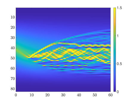
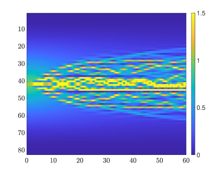
Figure 1. Colormap of intensity $|u_{j}|^{2}$ for evolution of Eq. 1 in $t$. Horizontal axis is $t$, vertical axis is lattice index $j$. Initial condition is $u_{j}=c_{j}e^{ij\phi}$, where $c_{j}$ is a piecewise linear ramp from 0 to 1 and back, defined by $u_{j}=2j/N$ for $0\leq j\leq N/2$ and $u_{j}=2-2j/N$ for $N/2\leq j\leq N$. $\phi=\pi/4$ (left) and $\phi=\pi/2$ (right). $N=80$ lattice sites, $d=0.25$.

Equation Eq. 1 is Hamiltonian, with conserved energy given by

$$H(u)=\sum_{j}\left(\frac{1}{4}|u_{j}|^{4}-\frac{d}{4}\left(\overline{u}_{j}^{2}u_{j-1}^{2}+u_{j}^{2}\overline{u}_{j-1}^{2}\right)\right),$$ (2)

which follows from translation symmetry of Eq. 1 in $t$. By the Cauchy-Schwarz inequality,

$$\frac{1-2d}{4}\sum_{j}|u_{j}|^{4}\leq H(u)\leq\frac{1+2d}{4}\sum_{j}|u_{j}|^{4},$$

which implies, in particular, that the Hamiltonian is coercive if $d\in(0,1/2)$ (it is then equivalent to the $\ell^{4}$ norm); we will see that it is useful to think of this case as defocusing. The power of the solution (squared $\ell^{2}$ norm)

$${}P(u)=\|u\|_{\ell^{2}}^{2}=\sum_{j}|u_{j}|^{2}$$

is also conserved, which follows from the gauge symmetry $u\mapsto e^{i\theta}u$ of Eq. 1. In addition, the model is invariant under the transformation $u\mapsto au$, $t\mapsto a^{3}t$, for a real constant $a$. As a consequence, scaling the amplitude of the solution does not qualitatively affect the solution but merely speeds up or slows down its time evolution. Finally, some “staggering transforms” act in an interesting way on the equation. The transform $u_{j}\mapsto\epsilon_{j}u_{j}$, where $\epsilon_{j}=\pm 1$, leaves the equation invariant. The transform $u_{j}\mapsto i^{j}u_{j}$ amounts to flipping the sign of $d$, which shows that the case $d<0$ is included in our analysis, thus we can take $d>0$ without loss of generality.

Defining the density matrix elements by

$$\rho_{jk}=u_{j}\overline{u_{k}},$$ (3)

the evolution equation for $\rho_{jk}$ is given by

$$\frac{d}{dt}\rho_{jk}=i \Big{[}d\left(\rho_{j-1,j}\rho_{j-1,k}+\rho_{j+1,j}\rho_{j+1,k}-\rho_{j,k-1}\rho_{k,k-1}-\rho_{j,k+1}\rho_{j,k+1}\right)$$ (4)

$$\quad+\left(\rho_{kk}-\rho_{jj}\right)\rho_{jk}\Big{]}.$$

The intensity at lattice site $j$ is given by $\rho_{jj}=|u_{j}|^{2}$, which has evolution

$$\frac{d}{dt}\rho_{jj} =id\left(\rho_{j-1,j}^{2}+\rho_{j+1,j}^{2}-\rho_{j,j-1}^{2}-\rho_{j,j+1}^{2}\right)$$ (5)

$$=-2d\mathop{\mathrm{missing}}{Im}\nolimits\left(\rho_{j-1,j}^{2}+\rho_{j+1,j}^{2}\right),$$

where we used the fact that $\rho_{jk}=\overline{\rho_{kj}}$. We can also separate real and imaginary parts by writing $u_{j}=a_{j}+ib_{j}$ for real $a_{j}$ and $b_{j}$. Equation Eq. 1 can then be written as

$$\frac{d}{dt}\begin{pmatrix}a_{j}\\ b_{j}\end{pmatrix}=\begin{pmatrix}(a_{j}^{2}+b_{j}^{2})b_{j}-2da_{j}(a_{j-1}b_{j-1}+a_{j+1}b_{j+1})+db_{j}(a_{j-1}^{2}+a_{j+1}^{2}-b_{j-1}^{2}-b_{j+1}^{2})\\ -(a_{j}^{2}+b_{j}^{2})a_{j}+2db_{j}(a_{j-1}b_{j-1}+a_{j+1}b_{j+1})+da_{j}(a_{j-1}^{2}+a_{j+1}^{2}-b_{j-1}^{2}-b_{j+1}^{2})\end{pmatrix}.$$

This form of the equation is useful for numerical analysis, as well as for the linear stability analysis in subsection 4.5 below.

The system Eq. 1 can be posed either on the full integer lattice or on a finite lattice comprising $N$ nodes. Since equation Eq. 1 can be written as

$$\dot{u}_{j}=i\left[d(u_{j-1}^{2}+u_{j+1}^{2})-u_{j}^{2}\right]\overline{u_{j}},$$ (6)

it follows that if $u_{j}(0)=0$, then $u_{j}(t)=0$ for all $t>0$. If the initial data on the full integer lattice is nonzero only at a finite number of lattice sites, the system is equivalent to one on a finite lattice. In other words, intensity cannot spread to sites which are initialized to 0 (or bypass these sites), which is a feature fundamentally different from the linear dispersion case.

3. Modulational instability

We now turn to an analysis of modulational instability (MI) in the model, in order to further motivate the wave features which we will subsequently explore. Plane wave solutions of Eq. 1 can be found in the form

$$u_{j}(t)=Be^{i(kj-\omega t)},$$

with $k\in[-\pi,\pi]$. Substituting this into equation Eq. 1, plane waves satisfy the dispersion relation

$$\omega=|B|^{2}(1-2d\cos(2k)).$$

To understand the stability of such plane waves, we perturb according to

$$u_{j}(t)=Be^{i(kj-\omega t)}(1+a_{j}(t)).$$

Linearizing in $a_{j}$ (and using the dispersion relation) leads to the equation

$$-i\partial_{t}a_{j}=\omega(a_{j}-\overline{a_{j}})+|B|^{2}(-2a_{j}+2de^{2ik}a_{j+1}+2de^{-2ik}a_{j-1}).$$

Taking the Fourier transform normalized as

$$\widehat{a}(\theta)=\sum a_{j}e^{-i\theta j},$$

with $\theta\in[0,2\pi]$ being the wavenumber of the perturbation, this becomes

$$-i\partial_{t}\widehat{a}(\theta)=\omega(\widehat{a}(\theta)-\overline{\widehat{a}(-\theta)})+|B|^{2}(-2+4d\cos(2k+\theta))\widehat{a}(\theta).$$

This can be written as the vector equation

$$-i\partial_{t}A=MA$$

with $A=\widehat{a}(\theta)/\,\overline{\widehat{a}(-\theta)}$ and

$$M=\begin{pmatrix}|B|^{2}(-2+4d\cos(2k+\theta))+\omega&-\omega\\ \omega&-|B|^{2}(-2+4d\cos(2k-\theta))+\omega\end{pmatrix}.$$ (7)

Stability is then equivalent to the matrix $M$ having real eigenvalues, or, in other words

$$(\cos(2k+\theta)+\cos(2k-\theta)-2\cos(2k))(-1+d\cos(2k+\theta)+d\cos(2k-\theta))>0.$$ (8)

Using standard trigonometric identities, this criterion simplifies to

$$h(\theta)=2\cos(2k)(\cos\theta-1)(2d\cos(2k)\cos\theta-1)>0,$$ (9)

which is quadratic in $\cos\theta$ for fixed $d$ and $k$. Equation Eq. 9 always has a root at $\theta=0$; for $\qquad|2d\cos(2k)|\geq 1$, it has an additional pair of roots at

$$\theta=\pm\arccos\left(\frac{1}{2d\cos(2k)}\right).$$

Given the dependence of these expressions on $\cos\theta$, we can restrict the discussion (by mirror symmetry) to $\theta>0$ hereafter.

As an example, the left panel of Figure 2 plots $h(\theta)$ from Eq. 9 vs. $\theta$ for $k=\pi/8$. (The specific wavenumber is chosen so that the periodic boundary conditions on a lattice of size $N=256$ nodes are satisfied.) The roots of $h(\theta)$ are at 0 and $\pm\pi/4$, thus $h(\theta)$ is negative for $\pi/4<\theta<0$ and $0<\theta<\pi/4$, which is MI region. Compare the evolution of the two perturbations in the center panel of Figure 2; the perturbation with $\theta=\pi/6$ (solid blue line) is within the MI region and grows exponentially, in contrast to the perturbation with $\theta=\pi/2$ (dotted orange line), which is outside the MI region and thus does not grow. A colormap showing regions of MI in the $(\theta,k)$ plane is shown in the right panel of Figure 2; the color indicates the growth rate of MI, as given by the maximal imaginary part of the eigenvalues of Eq. 7. Two interesting observations here are as follows. First, MI is not always (and in particular is not for $k=0$) a long-wavelength instability with a band starting at $\theta=0$, as is typically the case in NLS models. Second, there are regions of modulationally stable wavenumbers $k$.

Colormaps showing the evolution of MI for all lattice sites are shown in Figure 3; comparison of these to the evolution plots in Figure 1 suggests that MI plays a significant role in the dynamics of this system. Importantly, the astute reader can discern a number of both standing and moving waves in the pattern that results from the MI. It is to these coherent structures that we now turn in more detail in what follows.

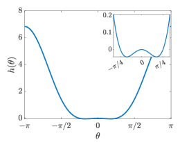
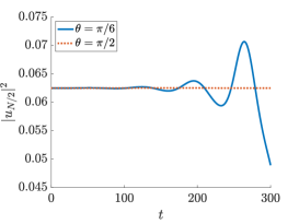
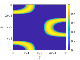
Figure 2. Left: plot of $h(\theta)$ from Eq. 9 vs. $\theta$ for $k=\pi/8$. Center: Evolution of the perturbation of plane wave using the initial condition $u_{j}(0)=Be^{ikj}(1+\epsilon e^{-i\theta j})$ with $\epsilon=0.0001$ and $B=1/4$ for $k=\pi/8$. Right: Regions of MI in the $(\theta,k)$ plane; intensity of colormap is maximum imaginary part of matrix $M$ from Eq. 7. The plot can be extended to negative $\theta$ and $k$ by symmetry. $d=1$ for all plots.

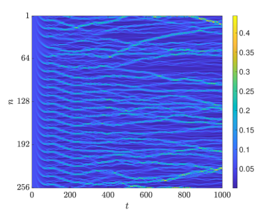
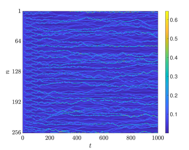
Figure 3. Evolution of perturbation of a plane wave using initial condition $u_{j}(0)=Be^{ikj}(1+\epsilon e^{-i\theta j})$ with $\epsilon=0.0001$ and $B=1/4$ for $k=\pi/8$, $\theta=\pi/6$ (left) and $k=\pi/2$, $\theta=\pi/6$ (right). For all plots, $N=256$ lattice nodes with periodic boundary conditions and $d=1$.

4. Standing Waves: Compactons

The first nonlinear structures of interest are compactons, which are standing waves supported on a finite set of $N$ adjacent lattice sites. (These also appear in different nonlinearly dispersive DNLS variants in, e.g., [vvk1, vvk2, vvk3], as discussed earlier.) Standing waves are solutions of the form

$$u_{j}=c_{j}e^{-i\omega t},$$ (10)

with frequency $\omega$ and amplitudes $c_{j}$. Although these amplitudes are traditionally real (as in, for example, the DNLS equation), we will see below that there is a class of solutions (the staggered compactons) where this is not the case.

4.1. Real compactons

Real compactons are solutions of the form Eq. 10, where all the $c_{j}$ are taken to be real. In this case, substituting Eq. 10 into Eq. 1 and simplifying, we obtain the standing wave equation

$$d(c_{j-1}^{2}+c_{j+1}^{2})c_{j}-c_{j}^{3}+\omega c_{j}=0.$$ (11)

For a compacton comprising $N$ sites labeled $c_{1}$ to $c_{N}$, since $c_{j}\neq 0$ for all $j$, we can divide equation Eq. 11 by $c_{j}$ to obtain

$$\begin{pmatrix}1&-d\\ -d&1&-d\\ &-d&1&-d\\ &&\ddots&\ddots&\ddots\\ &&&-d&1&-d\\ &&&&-d&1\end{pmatrix}\begin{pmatrix}c_{1}^{2}\\ c_{2}^{2}\\ c_{3}^{2}\\ \vdots\\ c_{N-1}^{2}\\ c_{N}^{2}\end{pmatrix}=\begin{pmatrix}\omega\\ \omega\\ \omega\\ \vdots\\ \omega\\ \omega\end{pmatrix},$$ (12)

which is linear in the square amplitudes $c_{j}^{2}$ and can be solved by row reduction. See Figure 4 for representative compacton solutions. We note that we can take either the positive or the negative root for each amplitude $c_{j}$.

For $N=1$, the compacton is a single-site standing wave $u_{1}=c_{1}e^{-i\omega t}$, with $c_{1}=\pm\sqrt{\omega}$. For $N=2,3,4$, and $5$, solving this linear system yields the solutions from Table 1. For fixed $\omega>0$, the norm of these solutions blows up as $d$ approaches $1$, $1/\sqrt{2}$, $(\sqrt{5}-1)/2$, and $1/\sqrt{3}$ (respectively) from below; the matrix in Eq. 12 is singular at these values of $d$. For a given $\omega$, since we are assuming the amplitudes $c_{j}$ are real, a compacton solution exists only if all of the square amplitudes $c_{j}^{2}$ are positive (see the intervals of existence in Table 1); this depends on whether $\omega>0$ or $\omega<0$. For example, for $N=2$, a real compacton exists on $(0,1)$ for $\omega>0$ and on $(1,\infty)$ for $\omega<0$. Interestingly, the 2-site compacton is spectrally stable on both of these intervals (See subsection 4.5.1 below for further discussion of stability; we note here that spectral stability does not change at the existence thresholds in Table 1 where the norm of the solution blows up).

For $N=2$ and $N=3$, the matrix in Eq. 12 is only singular at the values of $d$ already discussed. For $N\geq 4$, however, the matrix is singular at other values of $d$. For example, when $N=4$, the matrix is singular when $d=(\sqrt{5}+1)/2$. At this value of $d$, the solution in Table 1 exists but is not unique; we can add any multiple of the kernel vector $(d,1,-1,-d)$ to obtain another solution. The case when $N=5$ is similar. The matrix in Eq. 12 is singular when $d=1$, in which case we can add any multiple of the kernel vector $(1,1,0,-1,-1)$ to get another solution. (See subsection 4.5.1 below for a discussion on how spectral stability changes at these singular points.) In addition, for $N=5$, real compactons do not exist when $d>(1+\sqrt{5})/2$, since, in that case, $c_{1}^{2}$ and $c_{2}^{2}$ have opposite signs for all $\omega$. For larger $N$, analytic computation of exact solutions is less straightforward. Numerical computation strongly suggests that real compactons of all sizes $N$ exist for $0<d<1/2$. Existence results for compactons for $d$ outside this interval are more complicated. (The blue filled circles in Figure 6 indicate which compactons exist for a few values of $d>1/2$.) Finally, we note that the real compacton solutions are characterized by a plateau in the center of the solution. For $0<d<1/2$, the height of this plateau approaches

$$c^{2}=\frac{\omega}{1-2d}$$ (13)

for large $N$, which is found by taking $c_{j}=c_{j-1}=c_{j+1}=c$ in Eq. 11 and solving for $c$.

$N$	real compacton solution			$\omega>0$	$\omega<0$
2	$c_{1}^{2},\,c_{2}^{2}=\frac{\omega}{1-d}$			$(0,1)$	$(1,\infty)$
3	$c_{1}^{2},\,c_{3}^{2}=\frac{\omega(1+d)}{1-2d^{2}}$	$c_{2}^{2}=\frac{\omega(1+2d)}{1-2d^{2}}$		$\left(0,\frac{1}{\sqrt{2}}\right)$	$\left(\frac{1}{\sqrt{2}},\infty\right)$
4	$c_{1}^{2},\,c_{4}^{2}=\frac{\omega}{1-d-d^{2}}$	$c_{2}^{2},\,c_{3}^{2}=\frac{\omega(1+d)}{1-d-d^{2}}$		$\left(0,\frac{\sqrt{5}-1}{2}\right)$	$\left(\frac{\sqrt{5}-1}{2},\infty\right)$
5	$c_{1}^{2},\,c_{5}^{2}=\frac{\omega(1+d-d^{2})}{1-3d^{2}}$	$c_{2}^{2},\,c_{4}^{2}=\frac{\omega(1+2d)}{1-3d^{2}}$	$c_{3}^{2}=\frac{\omega(1+d)^{2}}{1-3d^{2}}$	$\left(0,\frac{1}{\sqrt{3}}\right)$	$\left(\frac{1}{\sqrt{3}},\frac{\sqrt{5}+1}{2}\right)$

Table 1. Square amplitudes for real compacton solutions for $N=2,3,4$ and $5$, together with intervals of existence for these solutions for $\omega>0$ and $\omega<0$.

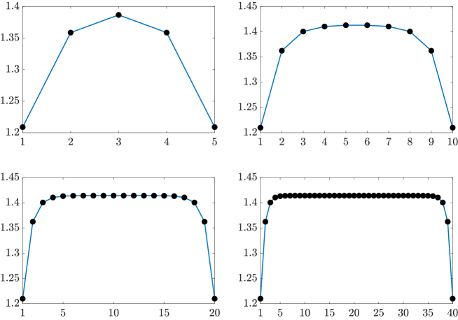
Figure 4. Compacton solutions for $N=5,10,20,40$. Positive amplitude $c_{j}$ is chosen at each site, $d=0.25$, $\omega=1$.

To better understand the solutions of the above linear problem, we observe first that it suffices to consider the case $\omega=1$. Denoting $M$ for the matrix in Eq. 12, $\mathbf{x}$ for the vector $(c_{j}^{2})$ and $\mathbf{1}$ for the vector $(1,\dots,1)^{\top}$, equation Eq. 12 becomes

$$M\mathbf{x}=\mathbf{1}.$$

Since $M$ is a tridiagonal Toeplitz matrix, its eigenvalues $\lambda_{k}$ and eigenvectors $\mathbf{e}_{k}$ can be computed explicitly (see for instance [Smith1985], page 154):

$$\lambda_{k}=1-2d\cos\left(\frac{k\pi}{N+1}\right),\qquad\mathbf{e}_{k}=\left(\sin\left(\frac{kj\pi}{N+1}\right)\right)_{j=1,\dots,N}\qquad\mbox{$k=1\dots N$.}$$

For $d\in(0,1/2)$, the eigenvalues $\lambda_{k}$ are positive, and the matrix $M$ is an $M$-matrix; in particular its inverse has positive entries, so that $\mathbf{x}$ has positive entries.

Using trigonometric identities, we can then compute

$$\|\mathbf{e}_{k}\|^{2}=\sum_{j=1}^{N}\sin\left(\frac{kj\pi}{N+1}\right)^{2}=\frac{N}{2}-\frac{1}{2}\sum_{j=1}^{N}\cos\left(\frac{2kj\pi}{N+1}\right)=\frac{N-1}{2}$$

$$\langle\mathbf{1},\mathbf{e}_{k}\rangle=\sum_{j=1}^{N}\sin\left(\frac{kj\pi}{N+1}\right)=\left\{\begin{array}[]{ll}0&\mbox{if $k$ even}\\ \mbox{cotan}\left(\frac{k\pi}{2(N+1)}\right)&\mbox{if $k$ odd}.\end{array}\right.$$

Since $M$ is self-adjoint, We can now invert the linear equation through the formula

$$\mathbf{x}=\sum_{k=1}^{N}\frac{1}{\|\mathbf{e}_{k}\|^{2}}\langle\mathbf{1},\mathbf{e}_{k}\rangle\mathbf{e}_{k}.$$

In other words, the coordinates of $\mathbf{x}$ are given by

$$x^{\ell}=\frac{2}{N-1}\sum_{\begin{subarray}{c}k\in 2\mathbb{N}-1\end{subarray}}\frac{1}{1-2d\cos\left(\frac{k\pi}{N+1}\right)}\mbox{cotan}\left(\frac{k\pi}{2(N+1)}\right)\sin\left(\frac{k\ell\pi}{N+1}\right),$$

We now want to find the limit as $N\to\infty$ of this expression, when $\ell$ is away from the extremities; we will assume that $\frac{\ell}{N}\to\alpha\in(0,1)$. In the above sum, the leading contribution is given by small $k$’s, due to the singularity at zero of the cotan function. Therefore, it is legitimate to expand in $\frac{k}{N}$, which gives

$$x^{\ell}\sim\frac{2}{n-1}\sum_{\begin{subarray}{c}k\in 2\mathbb{N}-1\end{subarray}}\frac{1}{1-2d}\frac{2(N+1)}{k\pi}\sin\left(\alpha k\pi\right)\sim\frac{4}{\pi(1-2d)}\sum_{\begin{subarray}{c}k\in 2\mathbb{N}-1\end{subarray}}\frac{\sin\left(\alpha k\pi\right)}{k}.$$

By the formula for the Fourier series of the sawtooth wave

$$\sum_{k=1}^{\infty}\frac{\sin(kx)}{k}=\frac{\pi}{2}-\frac{x}{2}$$

for $x\in(0,2\pi)$, we obtain for $\alpha\in(0,\pi)$

$$x^{\ell} \sim\frac{4}{\pi(1-2d)}\left[\sum_{k\in\mathbb{N}}\frac{\sin\left(\alpha k\pi\right)}{k}-\sum_{k\in\mathbb{N}}\frac{\sin\left(2\alpha k\pi\right)}{2k}\right]=\frac{1}{1-2d}.$$

This result suggests, in close correspondence with Figure 4, that the compacton solution becomes nearly flat in its center for sufficiently large $N$.

4.2. The staggered compacton

For solutions supported on $N$ sites, another standing wave solution is obtained by using the ansatz

$$u_{j}=i^{j}c_{j}e^{-i\omega t},$$

where the $c_{j}$ are again real. We call this a staggered compacton, since there is a phase difference of $\pi/2$ between each pair of adjacent sites. Substituting this ansatz into Eq. 1 and simplifying, the amplitudes $c_{j}$ solve the equation

$$-d(c_{j-1}^{2}+c_{j+1}^{2})c_{j}-c_{j}^{3}+\omega c_{j}=0,$$ (14)

which leads to the linear system

$$\begin{pmatrix}1&d\\ d&1&d\\ &d&1&d\\ &&\ddots&\ddots&\ddots\\ &&&d&1&d\\ &&&&d&1\end{pmatrix}\begin{pmatrix}c_{1}^{2}\\ c_{2}^{2}\\ c_{3}^{2}\\ \vdots\\ c_{N-1}^{2}\\ c_{N}^{2}\end{pmatrix}=\begin{pmatrix}\omega\\ \omega\\ \omega\\ \vdots\\ \omega\\ \omega\end{pmatrix}.$$ (15)

We note that these are the same equations as those satisfied by the real compacton, except that $d$ has been changed to $-d$. Staggered compacton solutions for small $N$ are shown in Table 2. Although the solutions from this table are obtained from those in Table 1 by replacing $d$ with $-d$, their intervals of existence are very different. Of note, for $\omega>0$, the 2-site compacton exists for all $d$; in particular, its norm does not blow up for any $d>0$. As with the real compacton case, numerical computations suggest that staggered compactons of all sizes $N$ exist for $0<d<1/2$. As with the real compacton, existence results are more complicated for $d>1/2$ (see the orange unfilled circles in Figure 6, which indicate compactons that exist for a few values of $d>1/2$).

$N$	staggered compacton solution			$\omega>0$
2	$c_{1}^{2},\,c_{2}^{2}=\frac{\omega}{1+d}$			$(0,\infty)$
3	$c_{1}^{2},\,c_{3}^{2}=\frac{\omega(1-d)}{1-2d^{2}}$	$c_{2}^{2}=\frac{\omega(1-2d)}{1-2d^{2}}$		$\left(0,\frac{1}{2}\right)$, $\left(1,\infty\right)$
4	$c_{1}^{2},\,c_{4}^{2}=\frac{\omega}{1+d-d^{2}}$	$c_{2}^{2},\,c_{3}^{2}=\frac{\omega(1-d)}{1+d-d^{2}}$		$\left(0,1\right)$
5	$c_{1}^{2},\,c_{5}^{2}=\frac{\omega(1-d-d^{2})}{1-3d^{2}}$	$c_{2}^{2},\,c_{4}^{2}=\frac{\omega(1-2d)}{1-3d^{2}}$	$c_{3}^{2}=\frac{\omega(1-d)^{2}}{1-3d^{2}}$	$\left(0,\frac{1}{2}\right)$

Table 2. Square amplitudes for staggered compacton solutions for $N=2,3,4$ and $5$, together with intervals of existence for these solutions for $\omega>0$ . These four solutions do not exist for $\omega<0$.

Plots of staggered compactons for the same values of $N$ as the real-valued compactons are shown in Figure 5. The staggered compacton has higher energy than the real compacton (Figure 6, left). There is an intensity plateau in the middle of the solution; for large $N$, this plateau approaches

$$c^{2}=\frac{\omega}{1+2d}$$ (16)

for $0<d<1/2$. As in the case of the real compacton, this corresponds to a solution $\mathbf{x}$ such that

$$x^{\ell}\to\frac{1}{1+2d}\qquad\mbox{as $N\to\infty$}.$$

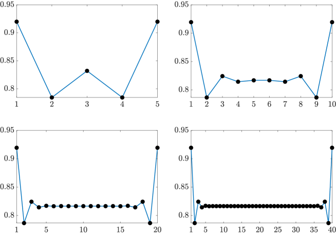
Figure 5. Staggered compacton solutions for $N=5,10,20,40$. Positive amplitude at each site, $d=0.25$, $\omega=1$.

4.3. Mixed compactons

The phase differences between adjacent lattice sites are 0 (or $\pi$, if negative roots are taken for the $c_{j}$) for real compactons and $\pi/2$ for staggered compactons. It is possible to construct compactons which have “mixed” phase differences. For example, for a 3-site compacton, we can take the ansatz

$$u_{1}=c_{1},\quad u_{2}=c_{2},\quad u_{3}=ic_{3},$$

where $c_{1}$, $c_{2}$, and $c_{3}$ are real. A compacton solution is then given by

$$c_{1}^{2}=\frac{\omega(1+d-2d^{2})}{1-2d^{2}},\quad c_{2}^{2}=\frac{\omega}{1-2d^{2}},\quad c_{3}^{2}=\frac{\omega(1-d-2d^{2})}{1-2d^{2}},$$

for $0<d<1/2$ (the square amplitudes $c_{j}^{2}$ are only all positive on this interval). This compacton is unstable. Indeed, numerical computations suggest that all such compactons are unstable, hence we will not consider such “mixed-phase” solutions hereafter.

4.4. Energy considerations

$N$	energy ($H$)
2	$\frac{\omega^{2}}{2(1-d)}=\frac{(1-d)P^{2}}{8}$
3	$\frac{(3+4d)\omega^{2}}{4(1-2d^{2})}=\frac{(1-2d^{2})P^{2}}{4(3+4d)}$
4	$\frac{(2+d)\omega^{2}}{2(1-d-d^{2})}=\frac{(1-d-d^{2})P^{2}}{8(2+d)}$
5	$\frac{(5+8d-d^{2})\omega^{2}}{4(1-3d^{2})}=\frac{(1-3d^{2})P^{2}}{4(5+8d-d^{2})}$

Table 3. Energy for real compacton solutions for $N=2,3,4$ and $5$ as a function of frequency $\omega$ or power of solution $P$. Energy for staggered compactons is found by replacing $d$ with $-d$. Single-site solution has energy $H=P^{2}/4$.

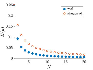
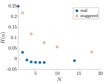
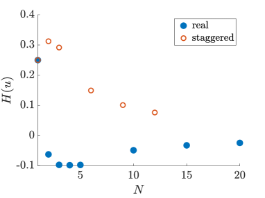
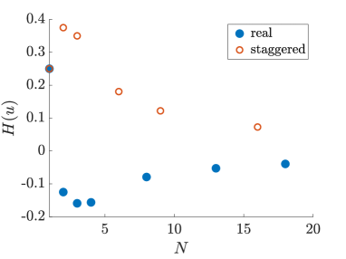
Figure 6. Energy $H$ for real and staggered compacton solutions scaled so that power $P=1$ for all solutions. $d=0.25,0.75,1.5$, and $2$ (top to bottom, left to right). For $d>1/2$, solutions for a particular $N$ do not exist if a marker is not shown.

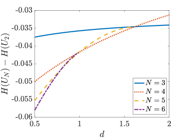
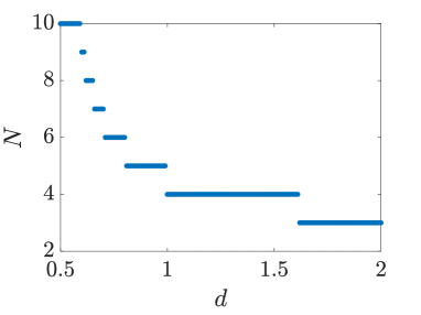
Figure 7. Right: Energy difference between compacton of size $N$ and compacton of size 2 vs. $d$. Left: size of compacton of minimum energy (selected only from among compactons of sizes from $N=1$ to $N=10$) vs. $d$. All solutions scaled so that power $P=1$. The value of $N$ selected for the given $d$ corresponds to the spatial extent of the ground state of the system.

The energy Eq. 2 of real and staggered compactons for various $N$ and $d$ is plotted in Figure 6 (the power of the solution is scaled to $1$ for all $N$). Formulas for the energy of small compactons are also given in Table 3. For $0<d<1/2$ and fixed power (exemplified by Figure 6, top left), the energy decreases monotonically with increasing $N$, both for real and staggered compactons. The staggered compacton has higher energy than the real compacton, although this difference becomes smaller with increasing $N$; the latter is natural to expect, as the profile of both compactons asymptotes to a constant near the center of the respective structure. For all $d$, the single-site solution (compacton with $N=1$) of power $P$ has energy $H=P^{2}/4$, which is independent of $d$. For $0<d<1$, this single-site solution is the energy maximum. The energy of the two-site staggered compacton is $(1+d)P^{2}/8$, which increases with increasing $d$, and surpasses the energy of the single site solution at $d=1$. For $d>1$, the two-site staggered compacton is the energy maximum. This implies that the two-site staggered compacton is stable for $d>1$ (see subsection 4.5.2 below). Numerical computations indicate that these solutions (single site solution if $d<1$ and two-site staggered compacton if $d>1$) maximize the Hamiltonian $H$ over all vectors in $\ell^{2}$, under the constraint that the power $P$ is fixed. Since $H$ and $P$ are conserved quantities of the system, this implies that both are stable in the sense of Lyapunov (for the appropriate value of $d$). Note that the growth mechanism exhibited in [Colliander2010] exploits the instability of the single site solution, which follows from the value $d=2$.

For $d>1/2$, numerical computations suggest that the energy minimizer is the real compacton of a finite size (which depends on $d$). See the left panel of Figure 7 for a plot of the energies of compactons of sizes $N=3,4,5$ and $6$ vs. $d$ (for ease of visualization, the vertical axis actually plots the energy difference with the 2-site compacton). This is further confirmed by performing a constrained minimization using Matlab’s fmincon function, with fixed power as the sole constraint; we note that we do not restrict ourselves to standing wave solutions. For $d=0.75$, 1.5, and 2, the energy minimizer is the real compacton comprising $N=6$, 4, and 3 sites, respectively. Numerical computations suggest that as $d$ is increased from $d=1/2$, the size of the compacton with energy minimum decreases until it reaches $N=4$ at $d=1$ and then finally $N=3$ at $d=(1+\sqrt{5})/2$ (see Figure 7, right, noting that only compactons with sizes of 10 and smaller are considered). The right panel of Figure 7 also suggests that as $d$ approaches 1/2 from above, the size of the compacton with minimum energy approaches infinity.

4.5. Linearization and stability

Linearizing about a standing wave of the form $(a_{j}+ib_{j})e^{-i\omega t}$, where $a_{j}$ and $b_{j}$ are real, we obtain the eigenvalue problem

$$\begin{pmatrix}\tilde{L}^{-}&L^{-}\\ -L^{+}&-\tilde{L}^{+}\end{pmatrix}\begin{pmatrix}v_{j}\\ w_{j}\end{pmatrix}=\lambda\begin{pmatrix}v_{j}\\ w_{j}\end{pmatrix}$$ (17)

where

$$\tilde{L}^{-}v_{j} =2[a_{j}b_{j}-d(a_{j-1}b_{j-1}+a_{j+1}b_{j+1})]v_{j}$$ (18)

$$\qquad+2d[(a_{j-1}b_{j}-a_{j}b_{j-1})v_{j-1}+(a_{j+1}b_{j}-a_{j}b_{j+1})v_{j+1}]$$

$$L^{-}w_{j} =[(a_{j}^{2}+3b_{j}^{2})+d(a_{j-1}^{2}+a_{j+1}^{2}-b_{j-1}^{2}-b_{j+1}^{2})-\omega]w_{j}$$

$$\qquad-2d[(a_{j-1}a_{j}+b_{j-1}b_{j})w_{j-1}+(a_{j+1}a_{j}+b_{j+1}b_{j})w_{j+1}]$$

$$L^{+}v_{j} =[(3a_{j}^{2}+b_{j}^{2})-d(a_{j-1}^{2}+a_{j+1}^{2}-b_{j-1}^{2}-b_{j+1}^{2})-\omega]v_{j}$$

$$\qquad-2d[(a_{j-1}a_{j}+b_{j-1}b_{j})v_{j-1}+(a_{j+1}a_{j}+b_{j+1}b_{j})v_{j+1}]$$

$$\tilde{L}^{+}w_{j} =2[a_{j}b_{j}-d(a_{j-1}b_{j-1}+a_{j+1}b_{j+1})]w_{j}$$

$$\qquad-2d[(a_{j-1}b_{j}-a_{j}b_{j-1})w_{j-1}+(a_{j+1}b_{j}-a_{j}b_{j+1})w_{j+1}]$$

For both the real and the staggered compacton, these linear operators simplify significantly. We treat these two cases separately below.

4.5.1. Real compactons

For a compacton solution $c_{j}e^{-i\omega t}$ where the amplitudes $c_{j}$ are real, the linear operators $\tilde{L}^{\pm}$ are 0, thus the eigenvalue problem becomes

$$\begin{pmatrix}0&L^{-}\\ -L^{+}&0\end{pmatrix}\begin{pmatrix}v_{j}\\ w_{j}\end{pmatrix}=\lambda\begin{pmatrix}v_{j}\\ w_{j}\end{pmatrix},$$ (19)

where

$$L^{-}w_{j} =(c_{j}^{2}+d(c_{j+1}^{2}+c_{j-1}^{2})-\omega)w_{j}-2dc_{j}(c_{j+1}w_{j+1}+c_{j-1}w_{j-1})$$

$$L^{+}v_{j} =(3c_{j}^{2}-d(c_{j+1}^{2}+c_{j-1}^{2})-\omega)v_{j}-2dc_{j}(c_{j+1}v_{j+1}+c_{j-1}v_{j-1}).$$

Since $d(c_{j-1}^{2}+c_{j+1}^{2})=c_{j}^{2}-\omega$ from Eq. 12, we can rewrite $L^{-}$ and $L^{+}$ as

$$L^{-}w_{j}=2(c_{j}^{2}-\omega)w_{j}-2dc_{j}(c_{j+1}w_{j+1}+c_{j-1}w_{j-1})$$

$$L^{+}v_{j}=2c_{j}^{2}v_{j}-2dc_{j}(c_{j+1}v_{j+1}+c_{j-1}v_{j-1}),$$

from which it follows that $L^{-}=L^{+}-2\omega I$. Furthermore, if we let $M$ be the matrix in Eq. 12, $L^{+}=2\,\text{diag}(c)\,M\,\text{diag}(c)$, where $\text{diag}(c)$ is the diagonal matrix with the amplitudes $c_{j}$ on the diagonal. The eigenvalues $\lambda$ do not depend on whether we take the positive or negative root for $c_{j}$. To see this, if $L^{+}$ is the matrix associated with a compacton with all positive amplitudes, and $\tilde{L}^{+}$ is the matrix associated with the same compacton, except the amplitude $c_{j}$ of site $j$ is negative, then $\tilde{L}^{+}=AL^{+}A$, where $A$ is the self-invertible matrix formed by changing the $j$th diagonal element of the identity matrix to $-1$.

Since the eigenvalue problem Eq. 19 can be written as $L^{-}L^{+}v=-\lambda^{2}v$, and the matrix $L^{-}L^{+}v=(L^{+}-2\omega I)L^{+}$ is symmetric, the eigenvalues of $L^{-}L^{+}$ are real, which implies that the eigenvalues $\lambda$ come in pairs which are either real or purely imaginary. For all $N$, there is an eigenvalue of algebraic multiplicity 2 and geometric multiplicity 1 at the origin due to the gauge symmetry of the system. For $N=1$, this double eigenvalue at $0$ is the only eigenvalue. For $N=2$, there is an additional pair of eigenvalues on the imaginary axis at

$$\lambda=\pm 2\omega\frac{\sqrt{2d(1+d)}}{1-d}i.$$

Since these are imaginary for both $0<d<1$ and $d>1$ (and for all $\omega$), the 2-site real compacton is spectrally stable. Perturbations of the 2-site real compacton yield oscillatory states which remain close to the unperturbed compacton (see subsection 4.5, in particular Figure 11). Exact formulas for eigenvalues are less straightforward to obtain (and present) for $N\geq 3$. Numerical computations suggest that the 3-site real compacton is spectrally stable for all $d>0$ and all $\omega$ for which it exists (see Table 1). Similarly, computations suggest that the 4-site real compacton is spectrally stable for $d\in\left(0,\frac{\sqrt{5}+1}{2}\right)$, and the 5-site real compacton is spectrally stable for $d\in(0,1)$. Stability is lost at the right endpoints of these intervals as a pair of imaginary eigenvalues collides at the origin and becomes real. We note that these endpoints coincide precisely with the additional values of $d$ at which the matrix in Eq. 12 is singular (see subsection 4.1 above). For $0<d<1/2$, numerical computations suggest that for all $N$, all of the nonzero eigenvalues are purely imaginary, which implies that real compactons of all sizes are spectrally stable in this parameter regime.

4.5.2. Staggered compactons

The staggered compacton alternates between sites which are real and site which are purely imaginary, thus all terms of the form $a_{j}b_{j}$, $a_{j}a_{j-1}$, $a_{j}a_{j+1}$, $b_{j}b_{j-1}$, and $b_{j}b_{j+1}$ are 0, which reduces the four linear operators in Eq. 18 to

$$\tilde{L}^{-}v_{j} =2d[(a_{j-1}b_{j}-a_{j}b_{j-1})v_{j-1}+(a_{j+1}b_{j}-a_{j}b_{j+1})v_{j+1})]$$

$$L^{-}w_{j} =[(a_{j}^{2}+3b_{j}^{2})+d(a_{j-1}^{2}+a_{j+1}^{2}-b_{j-1}^{2}-b_{j+1}^{2})-\omega]w_{j}$$

$$L^{+}v_{j} =[(3a_{j}^{2}+b_{j}^{2})-d(a_{j-1}^{2}+a_{j+1}^{2}-b_{j-1}^{2}-b_{j+1}^{2})-\omega]v_{j}$$

$$\tilde{L}^{+}w_{j} =-2d[(a_{j-1}b_{j}-a_{j}b_{j-1})w_{j-1}+(a_{j+1}b_{j}-a_{j}b_{j+1})w_{j+1}].$$

We note that for the staggered compacton, $\tilde{L}^{+}=-\tilde{L}^{-}$, and that both $L^{+}$ and $L^{-}$ are diagonal. As with the real compactons, there is an eigenvalue of algebraic multiplicity 2 and geometric multiplicity 1 at the origin due to the gauge symmetry of the system. For $N=2$, there is an additional pair of eigenvalues at

$$\lambda=\pm 2\omega\frac{\sqrt{2d(1-d)}}{1+d},$$

which are real when $0<d<1$, implying instability, and purely imaginary when $d>1$, implying spectral stability, with a bifurcation occurring at $d=1$. The behavior of perturbations to the 2-site staggered compacton can be fully understood using the phase portraits in Figure 11, noting that the staggered compacton corresponds to the fixed point at $(p,\phi)=(0,\pi/2)$ therein, where $p=|u_{2}|^{2}-|u_{1}|^{2}$ and $\phi$ is the phase difference between $u_{2}$ and $u_{1}$ (see subsection 5.3 below for details).

For $N\geq 3$, numerical eigenvalue computations suggest that for staggered compactons in the parameter regime $0<d<1/2$, all of the nonzero eigenvalues are real, thus the structures are all unstable. This instability is sufficiently strong that it can be demonstrated using numerical evolution experiments from unperturbed initial conditions (Figure 8). In general, these structures break down and do not tend towards or oscillate about any stable coherent structure. For example, for large $N$ (right panel of Figure 8), the staggered compacton solution breaks down into smaller structures similar to those seen in Figure 1. For small staggered compactons ($N=3$ and $N=4$) and particular values of $d$, however, the staggered compacton appears to decay into a coherent periodic orbit (Figure 9), but this behavior appears to be uncommon. For $N=3$, the periodic orbit in the top of Figure 9 has the symmetry $u_{3}=-u_{1}$, and the system Eq. 1 reduces to the pair of equations with asymmetric coupling terms

$$i\dot{u}_{1}+du_{2}^{2}\overline{u_{1}}-|u_{1}|^{2}u_{1}=0$$

$$i\dot{u}_{2}+2du_{1}^{2}\overline{u_{2}}-|u_{2}|^{2}u_{2}=0.$$

For $N=4$, the periodic orbit in the bottom of Figure 9 has the symmetry $u_{3}=iu_{2}$ and $u_{4}=-iu_{1}$, and the system reduces to the pair of equations with asymmetric nonlinear terms

$$i\dot{u}_{1}+du_{2}^{2}\overline{u_{1}}-|u_{1}|^{2}u_{1}=0$$

$$i\dot{u}_{2}+du_{1}^{2}\overline{u_{2}}-(1+d)|u_{2}|^{2}u_{2}=0.$$

Compare both of these cases to equation Eq. 20 for the symmetric dimer. Phase portraits of these periodic orbits are shown in the bottom panels of Figure 9, where $p=|u_{2}|^{2}-|u_{1}|^{2}$ and $\phi$ is the phase difference between $u_{2}$ and $u_{1}$ (see also subsection 5.3 below).

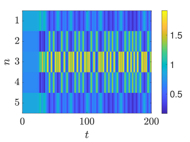
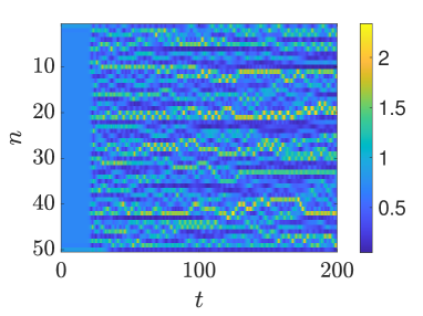
Figure 8. Colormap of square intensity $|u_{n}|^{2}$ of unperturbed staggered compactons with $N=5$ (left) and $N=50$ (right). $\omega=1$, $d=0.2$.

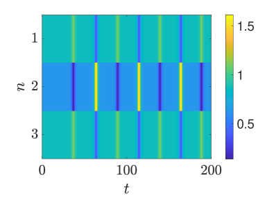
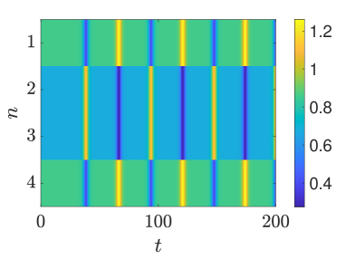
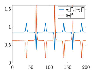
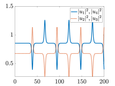
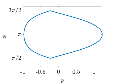
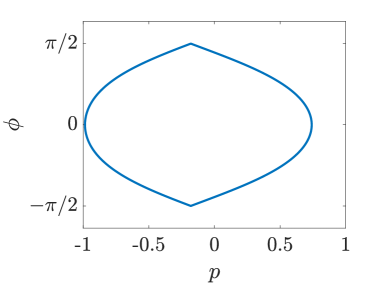
Figure 9. Top: colormap of square intensity $|u_{n}|^{2}$ of unperturbed staggered compactons. Middle: square intensity vs. $t$ of these solutions. Bottom: phase portraits corresponding to periodic orbits from the middle plots; $p=|u_{2}|^{2}-|u_{1}|^{2}$, and $\phi$ is the phase difference between $u_{2}$ and $u_{1}$. A “near-corner” occurs at the top and bottom of these periodic orbits as they pass very close to a saddle point equilibrium (compare to left panel of Figure 11). Left: $N=3$, $u_{3}=-u_{1}$ in periodic orbit. Right: $N=4$, $u_{3}=iu_{2}$ and $u_{4}=-iu_{1}$ in periodic orbit. $d=0.21$, $\omega=1$.

5. Dynamical considerations: the dimer case

Next, we look at solutions in which the intensity moves along the lattice. It turns out that a useful starting point is the dimer (two-site solution) on a periodic lattice:

$$i\dot{u}_{1}+2du_{2}^{2}\overline{u_{1}}-|u_{1}|^{2}u_{1}=0$$ (20)

$$i\dot{u}_{2}+2du_{1}^{2}\overline{u_{2}}-|u_{2}|^{2}u_{2}=0.$$

Note that if we take Dirichlet instead of periodic boundary conditions on the lattice, we replace $d$ with $d/2$ in Eq. 20. Numerical evolution experiments show that if one site is initialized to high intensity and the other to low intensity, optical intensity moves periodically between the two sites if $d>1/2$, but remains confined to the initial sites if $d<1/2$ (see Figure 10).

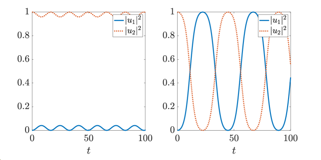
Figure 10. Evolution of dimer equation Eq. 20 on periodic lattice with initial conditions $u_{1}(0)=0.02$, $u_{2}(0)=1$. $d=0.49$ (left), $d=0.51$ (right). One can clearly discern the self-trapping transition occurring at $d=1/2$.

We can understand what is occurring by looking at the evolution of the four density matrix elements $\rho_{jk}=u_{j}\overline{u_{k}}$:

$$\dot{\rho}_{11}=2id\left(\rho_{21}^{2}-\rho_{12}^{2}\right) \quad\dot{\rho}_{12}=i\left(\rho_{22}-\rho_{11}\right)\left(2d\rho_{21}+\rho_{12}\right)$$ (21)

$$\dot{\rho}_{21}=-i\left(\rho_{22}-\rho_{11}\right)\left(2d\rho_{12}+\rho_{21}\right) \quad\dot{\rho}_{22}=-2id\left(\rho_{21}^{2}-\rho_{12}^{2}\right).$$

We note that in the degenerate case when one of the sites starts with zero intensity, e.g. $u_{2}(0)=0$, then $\rho_{22}(0)=\rho_{12}(0)=\rho_{21}(0)=0$, from which it follows that all four time derivatives in Eq. 21 are 0 for all $t\geq 0$. This implies that $u_{2}(t)=0$ for all $t>0$, thus we effectively have a single-site solution instead of a dimer. This is in line with our earlier comment regarding compactly supported initial data in this system. From here on, we assume both initial conditions are nonzero.

The analysis that follows is an adaptation of the method used in [Kenkre1986, ParkerPerMod]. We define

$$p=\rho_{22}-\rho_{11}\qquad q=i\left(\rho_{12}-\rho_{21}\right)\qquad r=\rho_{12}+\rho_{21}$$ (22)

$$s=(1-2d)q^{2}-(1+2d)r^{2}$$

where we note in particular that $p$ is the difference in intensity between the two sites in the dimer. Since

$$q=-2\mathop{\mathrm{missing}}{Im}\nolimits\rho_{12}\qquad\quad r=2\mathop{\mathrm{missing}}{Re}\nolimits\rho_{12},$$ (23)

all of these quantities are real. We can also write $s$ in terms of the density matrix elements as follows:

$$s =(q^{2}-r^{2})-2d(q^{2}+r^{2})$$ (24)

$$=-\left(\rho_{12}^{2}+\rho_{21}^{2}\right)-4d\rho_{12}\rho_{21}=-4\mathop{\mathrm{missing}}{Re}\nolimits\rho_{12}^{2}-8d|\rho_{12}|^{2}.$$

Letting

$$P=|u_{1}|^{2}+|u_{2}|^{2}=\rho_{11}+\rho_{22}$$

be the power of the solution, which is conserved in $t$, the intensities at the two lattice sites can be written in terms of $P$ and $p$ as

$$|u_{1}(t)|^{2}=\frac{1}{2}\left(P-p(t)\right)\qquad|u_{2}(t)|^{2}=\frac{1}{2}\left(P+p(t)\right).$$ (25)

We note that $|p(t)|\leq P$, and since we are not considering the degenerate case, the inequality will always be strict.

The time derivatives of $p$, $q$, $r$, and $s$ are given by

$$\dot{p}=4dqr \quad\dot{q}=-pr(1+2d)$$ (26)

$$\dot{r}=pq(1-2d) \quad\dot{s}=4(4d^{2}-1)pqr.$$

Since

$$\frac{d}{dt}\left(p^{2}\right)=2p\dot{p}=8dpqr,$$

the equation for $\dot{s}$ becomes

$$\dot{s}=\frac{4d^{2}-1}{2d}\frac{d}{dt}\left(p^{2}\right).$$

We can solve this to obtain

$$s=s_{0}+\frac{4d^{2}-1}{2d}\left(p^{2}-p_{0}^{2}\right),$$ (27)

where $p_{0}$ and $s_{0}$ are the initial conditions for $p$ and $s$. Since $\ddot{p}=4d\left(\dot{q}r+q\dot{r}\right)=4dps$, we obtain the second order differential equation for $p$

$$\ddot{p} =4dp\left[s_{0}+\frac{4d^{2}-1}{2d}\left(p^{2}-p_{0}^{2}\right)\right]$$

$$=\left[4ds_{0}-2(4d^{2}-1)p_{0}^{2}\right]p+2(4d^{2}-1)p^{3},$$

which we write as

$$\ddot{p}=(A-Bp_{0}^{2})p+Bp^{3},$$ (28)

where

$$A=4ds_{0},\qquad B=2(4d^{2}-1).$$

The two initial conditions are

$$p_{0}=p(0)=\rho_{22}(0)-\rho_{11}(0)$$ (29)

$$\dot{p}_{0}=\dot{p}(0)=4dq(0)r(0)=-8d\mathop{\mathrm{missing}}{Re}\nolimits\rho_{12}(0)\mathop{\mathrm{missing}}{Im}\nolimits\rho_{12}(0),$$

where the second line follows from Eq. 26 and Eq. 23.

The solutions for $p(t)$ will be in terms of Jacobi elliptic functions. To facilitate this, we look for a solution of the form

$$p(t)=Cy(Tt+\phi),$$ (30)

where the function $y$ will be a Jacobi elliptic function. Making this substitution and simplifying, equation Eq. 28 becomes

$$\ddot{y}=\frac{A-Bp_{0}^{2}}{T^{2}}y+\frac{BC^{2}}{T^{2}}y^{3}.$$ (31)

5.1. Real initial conditions

We first consider the case where the initial conditions $u_{1}(0)$ and $u_{2}(0)$ are both real. Using Eq. 25, the initial conditions for $q$, $r$, and $s$ are

$$q(0)=0\qquad r(0)=\sqrt{P^{2}-p_{0}^{2}}\qquad s(0)=-(1+2d)\sqrt{P^{2}-p_{0}^{2}},$$

from which it follows from Eq. 29 that $\dot{p}_{0}=0$. This in turn implies that $\phi=0$ and $C=p_{0}$ in Eq. 30. Equation Eq. 31 then becomes

$$\ddot{y}=-\frac{2(1+2d)(2dP^{2}-p_{0}^{2})}{T^{2}}y+\frac{2d(4d^{2}-1)p_{0}^{2}}{T^{2}}y^{3}.$$ (32)

If the two sites have identical initial intensity, i.e. $p_{0}=p(0)=0$, then $p(t)=0$ for all $t$. Otherwise, the solution is given by

$$p(t)=\begin{cases}p_{0}\,\text{dn}\left(\sqrt{1-4d^{2}}\,p_{0}t\,;m=m_{0}\right)&0<d<1/2,\left(\frac{p_{0}}{P}\right)^{2}>\frac{4d}{1+2d}\\ p_{0}\,\text{cn}\left(\sqrt{4d(1+2d)(P^{2}-p_{0}^{2})}t\,;m=\frac{1}{m_{0}}\right)&0<d<1/2,\left(\frac{p_{0}}{P}\right)^{2}<\frac{4d}{1+2d}\\ p_{0}\,\text{cd}\left(\sqrt{(1+2d)\left(4dP^{2}-(1+2d)p_{0}^{2}\right)}t\,;m=m_{1}\right)&d>1/2\end{cases}$$ (33)

where

$$m_{0}=\dfrac{4d}{1-2d}\left[\left(\dfrac{P}{p_{0}}\right)^{2}-1\right]\qquad m_{1}=\dfrac{(2d-1)p_{0}^{2}}{(2d-1)p_{0}^{2}+4d(P^{2}-p_{0}^{2})},$$

and we recall that $\text{cd}(t;m)=\text{cn}(t;m)/\text{dn}(t;m)$. For $d<1/2$, when $\left(\frac{p_{0}}{P}\right)^{2}=\frac{4d}{1+2d}$, $m=1$ in the first and second lines of Eq. 33, and the limiting solution is

$$p(t)=p_{0}\sech\left(\sqrt{1-4d^{2}}\,p_{0}t\right).$$ (34)

When $d=1/2$, $m=0$ in the second and third line of Eq. 33, and the limiting solution is

$$p(t)=p_{0}\cos\left(2\sqrt{P^{2}-p_{0}^{2}}\,t\right).$$

5.2. Equal intensity initial conditions

If $p_{0}=0$, i.e. the initial intensity at the two sites is identical, then the behavior of the system depends on $\dot{p}(0)$. If $\dot{p}_{0}\neq 0$, the solution $p(t)$ will not be 0 for all $t>0$. Let $u_{1}(0)=a$ and $u_{2}(0)=ae^{i\theta}$, where $a=\sqrt{P/2}>0$ and $\theta\in(-\pi,\pi)$. Due to the gauge symmetry, we can, without loss of generality, assume that $a$ is real and positive. The initial density matrix elements are given by

$$\rho_{11}(0)=\rho_{22}(0)=a^{2}\qquad\rho_{12}(0)=a^{2}e^{-i\theta}\qquad\rho_{21}(0)=a^{2}e^{i\theta},$$

and the initial conditions for $p$, $q$, $r$, and $s$ are $p(0)=0$ and

$$q(0)=P\sin\theta\qquad r(0)=P\cos\theta\qquad s(0)=-P^{2}(cos2\theta+2d),$$

where we used the formulas from Eq. 23 and Eq. 24. It follows from Eq. 26 that

$$\dot{p}(0)=4dq(0)r(0)=4dP^{2}\sin\theta\cos\theta=2dP^{2}\sin 2\theta.$$ (35)

If $\theta=0$ or $\theta=\pm\pi/2$, equation Eq. 35 implies that $\dot{p}(0)=0$, thus in those cases we will have $p(t)=0$ for all $t>0$. From here on, we will assume that $\theta\notin\{0,\pm\pi/2\}$.

Next, we define the constant $A_{0}$ by

$$A_{0}=1+2d\cos 2\theta.$$ (36)

In terms of $A_{0}$, the constant $A$ is given by

$$A=-4dP^{2}(\cos 2\theta+2d)=-2P^{2}\left[A_{0}+(4d^{2}-1)\right],$$

thus Eq. 28 becomes

$$\ddot{p}=-2P^{2}\left[A_{0}+(4d^{2}-1)\right]p+2(4d^{2}-1)p^{3}.$$

The solution depends on $d$ and the sign of $A_{0}$. We note if $d>1/2$, then we always have $A_{0}>0$.

$$p(t)=\begin{cases}\frac{dP\sin 2\theta}{\sqrt{d(1+2d\cos 2\theta)}}\,\text{sd}\left(2P\sqrt{d(1+2d\cos 2\theta)}\,t\,;m=\frac{(1-2d)\sin^{2}\theta}{1+2d\cos 2\theta}\right)&0<d<1/2\\ 2P\sin\theta\sqrt{\frac{d}{2d+1}}\,\text{sn}\left(2P\cos\theta\sqrt{d(2d+1)}\,t\,;m=\frac{2d-1}{2d+1}\tan^{2}\theta\right)&d>1/2,A_{0}>0\\ 2P\cos\theta\sqrt{\frac{d}{2d-1}}\,\text{sn}\left(2P\sin\theta\sqrt{d(2d-1)}\,t\,;m=\frac{2d+1}{2d-1}\cot^{2}\theta\right)&d>1/2,A_{0}<0,\end{cases}$$ (37)

where we recall that $\text{sd}(t;m)=\text{sn}(t;m)/\text{dn}(t;m)$. When $d=1/2$, $m=0$ in the first and second line of Eq. 37, and the limiting solution is

$$p(t)=P\sin\theta\sin\left((2P\cos\theta)t\right).$$

If $d>1/2$ and $A_{0}=0$, then $m=1$ in the second and third line of Eq. 37, and the limiting solution is

$$p(t)=P\tanh\left(P\sqrt{4d^{2}-1}\,t\right).$$ (38)

Using Eq. 25, the intensities at the two lattice sites are

$$|u_{1}(t)|^{2}=\frac{P}{1+e^{2P\sqrt{4d^{2}-1}t}}\qquad|u_{2}(t)|^{2}=\frac{P}{1+e^{-2P\sqrt{4d^{2}-1}t}}.$$ (39)

Taking $P=1$ and $d=1$, these are the slider solutions in [Colliander2010]*(3.7).

5.3. Dynamical system

Although the evolution of Eq. 20 occurs in a four-dimensional phase space comprising the real and imaginary parts of $u_{1}$ and $u_{2}$ (or, equivalently, the amplitude and phase of $u_{1}$ and $u_{2}$), we can reduce it to a two-dimensional dynamical system using the conservation of power and the gauge invariance of the system. To do this, we fix a power $P$, which will remain invariant as $t$ evolves. Writing $u_{1}=r_{1}e^{i\theta_{1}}$ and $u_{2}=r_{2}e^{i\theta_{2}}$, we will recast the system in the two dynamical variables

$$p=r_{2}^{2}-r_{1}^{2}\qquad\phi=\theta_{2}-\theta_{1},$$ (40)

where $p$ and $\phi$ are the intensity difference and phase difference, respectively, between $u_{1}$ and $u_{2}$. Using Eq. 20, we can derive the following dynamical system for $p$ and $\phi$:

$$\dot{p} =2d(P^{2}-p^{2})\sin 2\phi$$ (41)

$$\dot{\phi} =-p(1+2d\cos 2\phi),$$

where $p\in[-P,P]$ and $\phi\in(-\pi,\pi)$. (We note that the second-order ODE Eq. 28 for $p$ derived above, while less intuitive than Eq. 41, is much more useful for obtaining an exact solution for $p$). The system Eq. 41 is Hamiltonian, with conserved quantity $H$ given by

$$H(p,\phi)=\frac{1}{2}p^{2}-d(P^{2}-p^{2})\cos 2\phi,$$

and it can be written in standard Hamiltonian form as

$$\frac{dp}{dt}=\frac{\partial H}{\partial\phi},\qquad\frac{d\phi}{dt}=-\frac{\partial H}{\partial p}.$$

Equation Eq. 41 always has equilibria at $(0,0)$ and $(0,\pm\pi/2)$, which are the real compacton and the staggered compacton, respectively (see Figure 11). For $d>1/2$, there exist four additional pairs of equilibria (Figure 11, right) at $(\pm P,\phi_{*})$, where

$$\cos 2\phi_{*}=-\frac{1}{2d}.$$ (42)

At the bifurcation point ($d=1/2$), there are two entire lines of equilibria (blue lines in Figure 11, center) given by $(p,\pm\pi/2)$ for $p\in[-P,P]$; the endpoints of these lines satisfy Eq. 42, and the center points of these lines incorporate the equilibria at $(0,\pm\pi/2)$. For $d>1/2$, these lines become heteroclinic orbits connecting the equilibria $(\pm P,\phi_{*})$ (red lines in Figure 11, right).

Linearization about an equilibrium point $(p,\phi)$ yields the $2\times 2$ Jacobian matrix

$$\begin{pmatrix}-4dp\sin 2\phi&4d(P^{2}-p^{2})\\ -1-2d\cos 2\phi&4dp\sin 2\phi\end{pmatrix}.$$

The equilibrium at $(0,0)$ (corresponding to the real compacton) has a pair of eigenvalues $\lambda=\pm 2iP\sqrt{d(1+2d)}$; these are always imaginary, thus this equilibrium is a linear center (and, in fact, is a nonlinear center, since the system is Hamiltonian). The equilibria at $(0,\pm\pi/2)$ (corresponding to staggered compactons) have a pair of eigenvalues $\lambda=\pm 2P\sqrt{d(1-2d)}$, which are real for $0<d<1/2$ and imaginary for $d>1/2$. These equilibria are saddles for $0<d<1/2$ and centers for $d>1/2$; a bifurcation occurs at $d=1/2$. We note that for Dirichlet boundary conditions (where $d$ is replaced with $d/2$), this bifurcation takes place at $d=1$, which is consistent with subsection 4.5. When $d>1/2$, the four additional equilibria at $(\pm P,\phi_{*})$, where $\phi_{*}$ is defined by Eq. 42, are all saddles, since their eigenvalues are $\lambda=\pm 4dP\sin(2\phi_{*})$. It should be noted that the bifurcation at $d=1/2$ is responsible for the change from self-trapped dynamics (for $d<1/2$) to oscillatory behavior (for $d>1/2$) observed in Figure 10. For $d<1/2$, the manifolds of the saddle points at $(0,\pm\pi/2)$ prevent the orbit with strongly asymmetric initial data from oscillating with a changing sign of $p$, resulting in the observed self-trapped dynamics. On the contrary, the bifurcation at $d=1/2$ enables such large amplitude oscillations in $p$ past the critical point.

A phase portrait of this system is shown in Figure 11, and representative solutions are shown in Figure 12. When $0<d<1/2$, the limiting solutions Eq. 34 are heteroclinic orbits connecting the saddle points at $(0,-\pi/2)$ and $(0,\pi/2)$, which are depicted by red lines in the left panel of Figure 11. When $d>1/2$, the limiting solutions Eq. 38 are heteroclinic orbits connecting the saddles at $(-P,\phi_{*})$ and $(P,\phi_{*})$, with $\phi_{*}$ defined in Eq. 42. Note that $\dot{\phi}=0$, i.e., $\phi$ is constant, on these heteroclinic orbits, which are the red horizontal lines on the phase portrait in the right panel of Figure 11. These solutions are the sliders in [Colliander2010]; their highly unstable nature that has been observed in our dynamics can be explained by the phase portrait, since any perturbation (no matter how small) moves the solution onto one of the nearby periodic orbits. Indeed, depending on the nature of the perturbation, the resulting orbit may be confined to completely different regions of phase space, corresponding to very different values of the relative phase $\phi$.

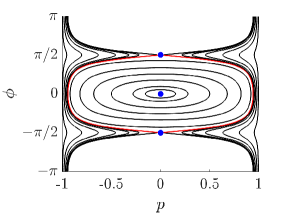
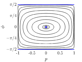
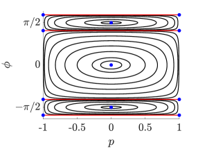
Figure 11. Phase portrait of the dynamical system Eq. 41. $d=0.4$ (left), 0.5 (center), and 0.6 (right). The red lines in the left and right panels are the limiting solutions Eq. 34 and Eq. 38, respectively. Equilibrium points are shown with blue dots, and the lines of equilibria for $d=1/2$ are blue solid lines. Power $P=1$.

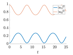
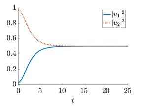
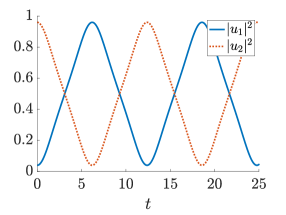
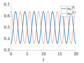
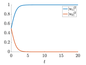
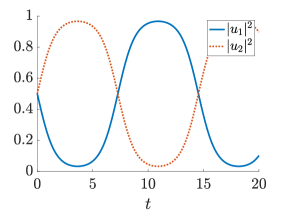
Figure 12. Representative solutions of dimer. Top row: $d=0.4<1/2$. Initial intensity $|u_{1}|^{2}$ is real and increases from left to right; solution Eq. 34 at bifurcation corresponds to red line in left panel of Figure 11. Bottom row: $d=0.6>1/2$. Initial intensity $|u_{1}|^{2}=|u_{2}|^{2}$, and initial phase difference $\phi$ increases from left to right; slider solution Eq. 38 at bifurcation corresponds to red line in right panel of Figure 11. Total power of solution is 1 in all cases.

6. Lattice traveling solutions

Motivated by the results we obtained from the dimer that showed the existence of solutions in which intensity is transferred between the two sites, we look for solutions in larger lattices in which the intensity flows unidirectionally along the lattice. In particular, we consider a lattice of $N$ nodes with periodic boundary conditions, i.e. the lattice is effectively a ring of $N$ nodes. We use a shooting method to find a solution in which the bulk of the intensity starts at the first lattice site at $t=0$, and then the entire solution reproduces itself exactly, except shifted one site to the right, at $t=1$. The choice of $t=1$ is arbitrary, but can be made without loss of generality due to the time-amplitude scaling from section 2; by symmetry, we can equivalently look for leftward-moving solutions. Thus we look to solve the boundary value problem

$$\dot{u}_{j} =i\left[d(u_{j-1}^{2}+u_{j+1}^{2})\overline{u_{j}}-|u_{j}|^{2}u_{j}\right] \qquad j=1,\dots,N$$ (43)

$$u_{j+1}(1) =u_{j}(0),$$

where the subscripts are taken $\mathop{\mathrm{missing}}{mod}\nolimits N$ due to the periodic lattice. In addition, due to the gauge symmetry, we can without loss of generality take $\mathop{\mathrm{missing}}{Im}\nolimits u_{1}(0)=0$. For the initial seed for the shooting method, we use the vector $(1,\epsilon,\dots,\epsilon)^{\top}$, where $\epsilon$ is small but nonzero. (We cannot take $\epsilon=0$, since sites which start at intensity of 0 will remain at 0 for all $t$). See Figure 13 for rightward moving solutions of varying $N$ computed numerically using this method. The solutions at each site are identical, except shifted by an integer time, thus they all satisfy the advance-delay equation

$$i\dot{u}(t)+d(u(t+1)^{2}+u(t-1)^{2})\overline{u(t)}-|u(t)|^{2}u(t)=0$$ (44)

for $t\in[0,N]$ with periodic boundary conditions. Once a solution has been obtained via a shooting method, equation Eq. 44 is useful for parameter continuation.

Representative moving solutions for four values of $N$ are shown in the top panel of Figure 13. Numerical experiments strongly suggest that these solutions only exist for $d>1/2$ (Figure 14, top left). Although the intensity profile of these moving solutions for sufficiently large $d$ (and $N$) are indicative of a localized solution on a constant background (solid blue line in Figure 14, top right), a plot of the real and imaginary parts of this solution (Figure 14, middle left) shows that the background is, in fact, not constant. As $d$ decreases towards 1/2, the difference between the minimum and maximum intensity decreases (Figure 14, top right), and the solution takes the form of oscillations on a constant background (Figure 14, middle right). Nevertheless, the relevant oscillation is only expected to disappear in the limit and is clearly found to persist in Figure 14 even close to that limit.

For exactly $d=1/2$, any constant state $u_{j}=C$, $j=1,\dots,N$, is a solution to Eq. 43. The parameter continuation in the top left of Figure 14 never reaches this constant limit at $d=1/2$, but it does come closer to it for larger lattice sizes. Furthermore, these solutions appear to only be spectrally stable (as defined by the Floquet multipliers being confined to the unit circle) for $d$ close to 1/2, i.e. for $1/2<d<d^{*}(N)$, where $d^{*}(N)$ approaches 1/2 as $N$ becomes large. The dynamical consequences of this can be observed in the lower panels of Figure 14 for $N=5$. For $d<d^{*}(5)$ (bottom left of Figure 14), the solution remains coherent for the 25 full periods shown in the figure (one period has a length in $t$ of 5, after which the system has returned exactly to its starting condition); in fact, numerical experiments show that it remains coherent for at least 1000 periods. By contrast, for $d>d^{*}(5)$, the solution breaks down after approximately 20 periods (Figure 14, bottom right).

These findings constitute, in our view, a significant addition to our understanding of such nonlinearly dispersive models. This is not only since, to our understanding, they have not been presented previously, but also because they appear to be central to segments of the dynamics that emerge in both our ramp (Figure 1) and in our modulationally unstable (Figure 3) dynamical evolutions.

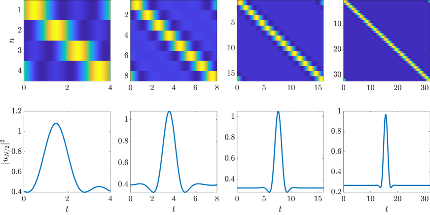
Figure 13. Colormap showing lattice site intensity (top) and intensity of central lattice site vs. $t$ (bottom) for rightward moving solutions on a periodic lattice for lattice sizes $N=4,8,16,32$. $d=0.6$.

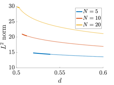
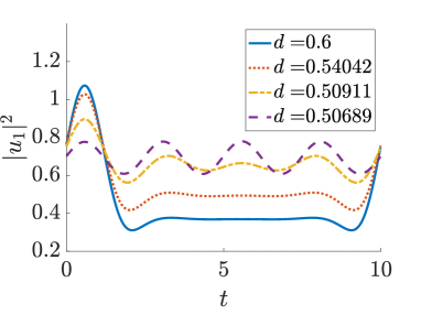
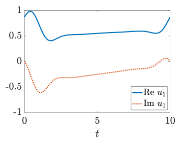
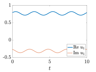
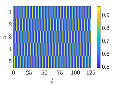
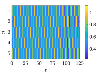
Figure 14. Top left: $L^{2}$ norm of $u_{1}(t)$ vs. $d$ for periodic lattice with $N=5,10$ and $20$; spectrally stable (unstable) solutions denoted by solid (dotted) lines. Top right: square intensities $|u_{1}(t)|^{2}$ of periodic moving solutions for $N=10$ and varying $d$. Middle: real and imaginary parts of $u_{1}(t)$ of periodic moving solutions from top left panel for $d=0.6$ (left) and $d=0.50689$ (right). Bottom: colormap of square intensity $|u_{n}|^{2}$ of evolution of unperturbed moving solutions on a periodic lattice with $N=5$, $d=0.537$ (left) and $d=0.555$ (right). $\omega=1$

7. Conclusions and Future Challenges

In the present work, we have revisited an intriguing minimal model characterized by the interplay of nonlinear dispersion and cubic nonlinearity. The motivation of the model stems from its derivation as a minimal description for the study of cascades across (groups of) Fourier modes in the defocusing NLS equation, which constitute the effective nodes of this lattice, that was initiated in the work of [Colliander2010]. This study adds to the wealth of earlier numerical [jeremy1, gideon2] and analytical [jeremy1, Her] explorations of this model by considering the prototypical nonlinear excitations thereof and their spectral stability properties, as well as their associated nonlinear dynamics. We found that the model exhibits different types of compactly supported nonlinear states, showcased their ranges of existence, and identified the termination and bifurcation points of the relevant structures. Both regular (monotonic) and staggered (non-monotonic) states were explored; for $d<1/2$, it was found that the former are spectrally stable, while the latter are spectrally unstable. We then turned to dynamical considerations and were able to analytically solve the simplest scenario thereof, namely the two-site (dimer); in addition, we were able to convert this problem into one involving only two degrees of freedom by using the relevant conservation laws. The phase portrait of this two-dimensional system captures the full dynamics of the dimer, explains the relevant bifurcations, and also sheds light on the subtle non-robustness of the so-called slider solutions discussed in [Colliander2010]. This, in turn, prompted us to search for generalizations of moving solutions in lattices with larger numbers of nodes, which we were able to identify. The somewhat unexpected (yet, a posteriori, justified) feature of such solutions was their apparent (for large lattice sizes) anti-dark nature, i.e., their density profiles that asymptoted to a constant nonzero value. While the states themselves are found to be unstable for large lattices, direct numerical simulations clearly illustrate their transient role in cascade dynamics and indeed motivated their direct numerical identification. Moreover we illustrated their potential stability near the parameter $d=1/2$.

This study motivates a wide range of additional questions worth examining. It might be useful to examine if analytical results can be extended beyond the dimer setting, e.g., into the trimer case of $N=3$, also potentially addressing the question of whether variants of slider states may be found therein. A deeper understanding of the transient role of the obtained traveling states in the dynamics and perhaps even more importantly in the thermodynamics and long time asymptotics [cretegny] of such nonlinear dispersive models would be particularly interesting to elucidate. While the relevance of this class of models as minimal models for turbulence is less evident in higher dimensions, their potential nonlinear wave patterns in the latter setting would be quite interesting to explore in their own right, motivated by the wealth of states accessible to higher dimensional linearly dispersive models [LEDERER20081]. Lastly, the implications of the present findings for continuum models of turbulence, while perhaps more removed from the current work, are certainly relevant to future thought and exploration.

Acknowledgments

This material is based upon work supported by the U.S. National Science Foundation under RTG Grants No. DMS-1840260 (R.P. and A.A.), No. PHY-2110030, No. DMS-2204702 (P.G.K.), and No. DMS-1909559 (A.A.). J.C.-M. acknowledges support from EU (FEDER Program No. 2014-2020) through MCIN/AEI/10.13039/501100011033 under Project No. PID2020-112620GB-I00. P.G. and P.G.K. gratefully acknowledge Professor Jeremy Marzuola for numerous informative discussions on the models considered herein.

Appendix A The continuous limit

The continuous or long wave limit, first considered in [jeremy1], is an important regime for the equation under consideration, and would deserve an investigation in its own right. We will not carry it out here, but will simply sketch some of its features. A key connection with the earlier developments in the present article has to do with the key value $d=1/2$, which arose repeatedly as a turning point. Namely, if one considers features such as variational properties, modulational stability, and stability of compactons, it makes sense to think of the cases $d<1/2$ (resp. $d>1/2$) as defocusing (resp. focusing). It is an interesting coincidence that $d=1/2$ also corresponds to the only value of $d$ for which the continuous limit asymptotically makes sense, as we will see below (compare to  [jeremy1, GHGM, jeremy2], which focus on the value $d=2$).

To investigate the continuous limit, we choose the ansatz

$$u_{j}(t)=u(t,hj)$$

where $u$ is a smooth function, $h>0$ (this is a slight abuse of notation; from now on, $u$ is a function on the real line instead of the lattice). Here, $u$ is a smooth function and $h>0$. Expanding in a Taylor series in $h$, one finds

$$i\partial_{t}u+(2d-1)|u|^{2}u+2h^{2}d\overline{u}\partial_{x}(u\partial_{x}u)+O(h^{3})=0.$$

The continuous limit corresponds to the case where

$$h\to 0,\quad\frac{2d-1}{2h^{2}}\to\alpha,$$

where $\alpha$ is a real constant (this implies in particular $d\to 1/2$). Upon rescaling time, the limiting equation is then

$$i\partial_{t}u+\alpha|u|^{2}u+\overline{u}\partial_{x}(u\partial_{x}u)=0.$$

A further rescaling enables one to restrict the value of $\alpha$ to $\alpha\in\{-1,0,1\}$. The Hamiltonian is now

$$H(u)=\frac{1}{2}\int|u\partial_{x}u|^{2}\,dx-\frac{\alpha}{4}\int|u|^{4}\,dx.$$

We now follow [GHGM] and seek solitary waves of the form

$$u(t,x)=Q(x-vt)e^{-ict},$$

where the wave profile $Q$ solves the ODE

$$cQ-ivQ^{\prime}+\overline{Q}(QQ^{\prime})^{\prime}+\alpha|Q|^{2}Q=0.$$

Multiplying by $\overline{Q}$ and taking the imaginary part, or multiplying by $\overline{Q^{\prime}}$ and taking the real part, one finds the two conservation laws

$$\frac{v}{2}|Q|^{2}+\text{Im}(|Q|^{2}\overline{Q}Q^{\prime})=\eta$$

$$-c|Q|^{2}+|Q|^{2}|Q^{\prime}|^{2}+\frac{\alpha}{4}|Q|^{4}=\kappa,$$

for constants $\eta$ and $\kappa$. In the particular case where $\eta=\kappa=0$, which correspond to localized waves, one finds that $Q=\psi e^{i\theta}$, where $\psi$ and $\theta$ solve the system of equations

$$c\psi=\psi(\psi\psi^{\prime})^{\prime}+\alpha\psi^{3}$$ (45)

$$\theta^{\prime}=-\frac{v}{2}\frac{1}{\psi^{2}}$$ (46)

The equation for $\psi$ can be integrated to give

$$c\psi^{2}=(\psi\psi^{\prime})^{2}+\frac{\alpha}{2}\psi^{4}+C,$$

for an integration constant $C$. If $C=0$, this can be integrated to give, up to translation

$$\psi=\sqrt{\frac{2c}{\alpha}}\sin\left(\sqrt{\frac{\alpha}{2}}(x-vt)\right),$$

which is valid for $\alpha=1$ or $d\rightarrow 1/2^{+}$. As one can see from the equation for the phase above, the solution fails to exist when $z=x-vt=n\pi$, as it creates a singularity in the phase, unless $v=0$, or the solution is stationary.

This result can be generalized for when $C\neq 0$. In that case, let $U=\psi^{2}$. Then $U$ satisfies the equation

$$2cU=(U^{\prime})^{2}+\alpha U^{2}+A$$

for a constant $A$. Completing squares and defining $W=U-\frac{c}{\alpha}$ we arrive at

$$(W^{\prime})^{2}=-\alpha W^{2}+\left[\left(\frac{c}{\alpha}\right)^{2}-A\right].$$

A solution to this is

$$U=\frac{c}{\alpha}\pm\sqrt{\frac{B}{\alpha}}\sin(\sqrt{\alpha}z+C),$$

for a constant $C$, where $B=\left(\frac{c}{\alpha}\right)^{2}-A$, thus $A<\left(\frac{c}{\alpha}\right)^{2}$. From the definition of $U$, only solutions that are non-negative are valid, restricting the choice of $B$ so that $\sqrt{\frac{B}{\alpha}}<\frac{c}{\alpha}$. Exploring the potential of constructing weak solutions out of a single period of these sinusoidal (static and traveling) waveforms, appropriately glued to a constant background (in the spirit of the compactons of [rosenau]) would constitute an interesting direction for future study.