Potential and limitations of random Fourier features for
dequantizing quantum machine learning

Abstract

Quantum machine learning is arguably one of the most explored applications of near-term quantum devices. Much focus has been put on notions of variational quantum machine learning where parameterized quantum circuits (PQCs) are used as learning models. These PQC models have a rich structure which suggests that they might be amenable to efficient dequantization via random Fourier features (RFF). In this work, we establish necessary and sufficient conditions under which RFF does indeed provide an efficient dequantization of variational quantum machine learning for regression. We build on these insights to make concrete suggestions for PQC architecture design, and to identify structures which are necessary for a regression problem to admit a potential quantum advantage via PQC based optimization.

1 Introduction

In recent years, the technique of using parameterized quantum circuits (PQCs) to define a model class, which is then optimized over via a classical optimizer, has emerged as one of the primary methods of using near-term quantum devices for machine learning tasks [CAB+21, BLS+19]. We will refer to this approach as variational quantum machine learning (variational QML), although it is often also referred to as hybrid quantum/classical optimization. While a large amount of effort has been invested in both understanding the theoretical properties of variational QML, and experimenting on trial datasets, it remains unclear whether variational QML on near-term quantum devices can offer any meaningful advantages over state-of-the-art classical methods.

One approach to answering this question is via dequantization. In this context, the idea is to use insights into the structure of PQCs, and the model classes that they define, to design quantum-inspired classical methods which can be proven to match the performance of variational QML. Ultimately, the goal is to understand when and why variational QML can be dequantized, in order to better identify the PQC architectures, optimization algorithms and problem types for which one might obtain a meaningful quantum advantage via variational QML.

In order to discuss notions of dequantization of variational QML, we note that for typical applications variational QML consists of two distinct phases. Namely, a training stage and an inference stage. In the training stage, one uses the available training data to identify an optimal PQC model, and in the inference stage one uses the identified model to make predictions on previously unseen data, or in the case of generative modelling, to generate new samples from the unknown data distribution.

A variety of works have recently proposed dequantization methods for inference with PQC models. The first such work was Ref. [SEM23], which used insights into the functional analytic structure of PQC model classes to show that, given a trained quantum model, one can sometimes efficiently extract a purely classical model – referred to as a classical surrogate – which performs inference just as well as the PQC model. More recently, Ref. [JGM+23] used insights from shadow tomography to show that it is sometimes possible to extract a classical shadow of a trained PQC model – referred to as a shadow model – which is again guaranteed to perform as well as the PQC model for inference. Interestingly, however, Ref. [JGM+23] also proved that, under reasonable complexity-theoretic assumptions, there exist PQC models whose inference cannot be dequantized by any efficient method – i.e., all efficient methods for the dequantization of PQC inference possess some fundamental limitations.

In this work, we are concerned with dequantization of the training stage of variational QML – i.e., the construction of efficient classical learning algorithms which can be proven to match the performance of variational QML in learning from data. To this end, we start by noting that Ref. [JGM+23] constructed a learning problem which admits an efficient variational QML algorithm but, again under complexity-theoretic assumptions, cannot be dequantized by any efficient classical learning algorithm. As such, we know that all methods for the dequantization of variational QML must posses some fundamental limitations, and for any given method we would like to understand its domain of applicability.

With this in mind, one natural idea is to ask whether the effect of noise allows direct efficient classical simulation of the the PQC model, and, therefore, of the entire PQC training process and subsequent inference. Indeed, a series of recent works has begun to address this question, and to delineate the conditions under which noise renders PQC models classically simulatable [FRD+22, FRD+23, SWC+23]. Another recent result has shown that the presence of symmetries, often introduced to improve PQC model performance for symmetric problems [MMG+23, LSS+22], can also constrain PQC models in a way which allows for efficient classical simulation [ABK+]. Another natural idea, inspired by the dequantization of inference with PQC models, is to “train the surrogate model”. More specifically, Ref. [SEM23] used the insight that the class of functions realizable by PQC models is a subset of trigonometric polynomials with a specific set of frequencies [SSM21], to “match” the trained PQC model to the closest trigonometric polynomial with the correct frequency set (which is then the classical surrogate for inference). This, however, immediately suggests the following approach to dequantizing the training stage of variational QML – simply directly optimize from data over the “PQC-inspired” model class of trigonometric polynomials with the appropriate frequency set. Indeed, this is in some sense what happens during variational QML! This idea was explored numerically in the original work on classical surrogates for inference [SEM23]. Unfortunately, for typical PQC architectures the number of frequencies in the corresponding frequency set grows exponentially with the problem size, which prohibits efficient classical optimization over the relevant class of trigonometric polynomials. However, for the PQC architectures for which numerical experiments were possible, direct classical optimization over the PQC-inspired classical model class yielded trained models which outperformed those obtained from variational QML.

Inspired by Ref. [SEM23], the subsequent work of Ref. [LTD+22] introduced a method for addressing the efficiency bottleneck associated with exponentially growing frequency sets. The authors of Ref. [LTD+22] noticed that all PQC models are linear models with respect to a trigonometric polynomial feature map. As such, one can optimize over all PQC-inspired models via kernel ridge regression, which will be efficient if one can efficiently evaluate the kernel defined from the feature map. While naively evaluating the appropriate kernel classically will be inefficient – again due to the exponential growth in the size of the frequency set – the clever insight of Ref. [LTD+22] was to see that one can gain efficiency improvements by using the technique of random Fourier features [RR07] to approximate the PQC-inspired kernel. Using this technique, Ref. [LTD+22] obtained a variety of theoretical results concerning the sample complexity required for RFF-based regression with the PQC-inspired kernel to yield a model whose performance matches that of variational QML. However, the analysis of Ref. [LTD+22] applied only to PQC architectures with universal parameterized circuit blocks – i.e., PQC models which can realize any trigonometric polynomial with the appropriate frequencies. This contrasts with the PQC models arising from practically relevant PQC architectures, which due to depth constraints, can only realize a subset of trigonometric polynomials.

In light of the above, the idea of this work is to further explore the potential and limitations of RFF-based linear regression as a method for dequantizing the training stage of variational QML, with the goal of providing an analysis which is applicable to practically relevant PQC architectures. In particular, we identify a collection of necessary and sufficient requirements – of the PQC architecture, the regression problem, and the RFF procedure – for RFF-based linear regression to provide an efficient classical dequantization method for PQC based regression. This allows us to show clearly that:

1. RFF-based linear regression cannot be a generic dequantization technique. At least, there exist regression problems and PQC architectures for which RFF-based linear regression can not efficiently dequantize PQC based regression. As mentioned before, we already knew from the results of Ref. [JGM+23] that all dequantization techniques must posses some limitations, and our results shed light on the specific nature of these limitations for RFF based dequantization.

2. There exist practically relevant PQCs, and regression problems, for which RFF-based linear regression can be guaranteed to efficiently produce output models which perform as well as the best possible output of PQC based optimization. In other words, there exist problems and PQC architectures for which PQC dequantization via RFF is indeed possible.

Additionally, using the necessary and sufficient criteria that we identify, we are able to provide concrete recommendations for PQC architecture design, in order to mitigate the possibility of dequantization via RFF. Moreover, we are able to identify a necessary condition on the structure of a regression problem which ensures that dequantization via RFF is not possible. This, therefore, provides a guideline for the identification of problems which admit a potential quantum advantage (or at least, cannot be dequantized via RFF-based linear regression).

This paper is structured as follows: We begin in Section 2 by providing all the necessary preliminaries and background material. Following this, we proceed in Section 3 to motivate and present RFF-based linear regression with PQC-inspired kernels as a method for the dequantization of variational QML. Given this, we then go on in Section 4 to provide a detailed theoretical analysis of RFF-based linear regression with PQC-inspired kernels. Finally, we conclude in Section 5 with a discussion of the consequences of the previous analysis, and with an overview of natural directions for future research.

2 Setting and preliminaries

Here we provide the setting and required background material.

2.1 Statistical learning framework

Let $\mathcal{X}$ denote a set of all possible data points, and $\mathcal{Y}$ a set of all possible labels. In this work, we will set $\mathcal{X}\coloneqq[0,2\pi)^{d}\subset\mathbb{R}^{d}$ for some integer $d$ and $\mathcal{Y}=\mathbb{R}$. We assume the existence of some unknown probability distribution $P$ over $\mathcal{X}\times\mathcal{Y}$, which we refer to as a regression problem. Additionally, we assume a parameterized class of functions $\mathcal{F}=\{f_{\theta}\colon\mathcal{X}\rightarrow\mathcal{Y}\,|\,\theta\in\Theta\}$, which we call hypotheses. Given access to some finite dataset $S=\{(x_{i},y_{i})\sim P\}|_{i=1}^{n}$ the goal of the regression problem specified by $P$ is to identify the optimal hypothesis $f_{\theta^{*}}$, i.e., the hypothesis which minimizes the true risk, defined via

$$R(f)\coloneqq\mathop{\mathbb{E}}_{(x,y)\sim P}\left[\mathcal{L}(y,f(x))\right],$$ (1)

where $\mathcal{L}\colon\mathcal{Y}\times\mathcal{Y}\rightarrow\mathbb{R}$ is some loss function. In this work, we will consider only the quadratic loss defined via

$${\mathcal{L}(y,y^{\prime})\coloneqq(y-y^{\prime})^{2}}.$$ (2)

We also define the empirical risk with respect to the dataset $S$ as

$$\hat{R}(f)\coloneqq\frac{1}{n}\sum_{i=1}^{n}\mathcal{L}(y_{i},f(x_{i})).$$ (3)

2.2 Linear and kernel ridge regression

Linear ridge regression and kernel ridge regression are two popular classical learning algorithms. In linear ridge regression we consider linear functions $f_{w}(x)=\langle w,x\rangle$, and given a dataset $S=\{(x_{i},y_{i})\}|^{n}_{i=1}$, we proceed by minimizing the empirical risk, regularized via the $2$-norm, i.e.,

$$\hat{R}_{\lambda}(f_{w})\coloneqq\frac{1}{n}\sum_{i=1}^{n}\left(y_{i}-\langle w,x_{i}\rangle\right)^{2}+\lambda\|w\|_{2}^{2}.$$ (4)

With this regularization, which is added to prevent over-fitting, minimizing Eq. (4) becomes a convex quadratic problem, which admits the closed form solution

$$w=\left(\hat{X}^{T}\hat{X}+\lambda n\mathds{1}\right)^{-1}\hat{X}^{T}\hat{Y},$$ (5)

where $\hat{X}$ is the $n\times d$ “data matrix” with $x_{i}$ as rows, and $\hat{Y}$ is the $n$ dimensional “target vector” with $y_{i}$ as the $i$’th component [MRT18]. Linear ridge regression requires $\mathcal{O}(nd)$ space and $\mathcal{O}(nd^{2}+d^{3})$ time. As linear functions are often not sufficiently expressive, a natural approach is to consider linear functions in some higher dimensional feature space. More specifically, one assumes a feature map $\phi\colon\mathbb{R}^{d}\rightarrow\mathbb{R}^{D}$, and then considers linear functions of the form $f_{v}(x)=\langle v,\phi(x)\rangle$, where $v$ is an element of the feature space $\mathbb{R}^{D}$. Naively, one could do linear regression at a space and time cost of $\mathcal{O}(nD)$ and $\mathcal{O}(nD^{2}+D^{3})$, respectively. However, often we would like to consider $D$ extremely large (or infinite) and this is therefore infeasible. The solution is to use “the kernel trick” and consider instead a kernel function $K\colon\mathcal{X}\times\mathcal{X}\rightarrow\mathbb{R}$ which satisfies

$$K(x,x^{\prime})=\langle\phi(x),\phi(x^{\prime})\rangle,$$ (6)

but which can ideally be evaluated more efficiently than by explicitly constructing $\phi(x)$ and $\phi(x^{\prime})$ and taking the inner product. Given such a function, we know that the minimizer of the regularized empirical risk is given by

$$f_{\alpha}(x) =\sum_{i=1}^{n}\alpha_{i}K(x_{i},x)$$ (7)

$$=\left\langle\sum_{i=1}^{n}\alpha_{i}\phi(x_{i}),\phi(x)\right\rangle$$ (8)

$$=\langle v,\phi(x)\rangle,$$ (9)

where

$$\alpha=\left(\hat{K}+n\lambda\mathds{1}\right)^{-1}\hat{Y},$$ (10)

with $\hat{K}$ the kernel matrix (or Gram matrix) with entries $\hat{K}_{i,j}=K(x_{i},x_{j})$. Solving Eq. (10) is known as kernel ridge regression. If one assumes that evaluating $K(x,x^{\prime})$ requires constant time, then kernel ridge regression has space and time cost $\mathcal{O}(n^{2})$ and $\mathcal{O}(n^{3})$, respectively. We note that in practice one hardly ever specifies the feature map $\phi$, and instead works directly with a suitable kernel function $K$.

2.3 Random Fourier features

For many applications, in which $n$ can be extremely large, a space and time cost of $\mathcal{O}(n^{2})$ and $\mathcal{O}(n^{3})$, respectively, prohibits the implementation of kernel ridge regression. This has motivated the development of methods which can bypass these complexity bottlenecks. The method of random Fourier features (RFF) is one such method [RR07]. To illustrate this method we follow the presentation of Ref. [RR17], and start by assuming that the kernel $K\colon\mathcal{X}\times\mathcal{X}\rightarrow\mathbb{R}$, has an integral representation. More specifically, we assume there exists some probability space $(\Phi,\pi)$ and some function $\psi\colon\mathcal{X}\times\Phi\rightarrow\mathbb{R}$ such that for all $x,x^{\prime}\in\mathcal{X}$ one has that

$$K(x,x^{\prime})=\int_{\Phi}\psi(x,\nu)\psi(x^{\prime},\nu)\,\mathrm{d}\pi(\nu).$$ (11)

The method of random Fourier features is then based around the idea of approximating $K(x,x^{\prime})$ by using Monte-Carlo type integration to perform the integral in Eq. (11). More specifically, one uses

$$K(x,x^{\prime})\approx\langle\tilde{\phi}_{M}(x),\tilde{\phi}_{M}(x^{\prime})\rangle$$ (12)

where $\tilde{\phi}_{M}\colon\mathcal{X}\rightarrow\mathbb{R}^{M}$ is a randomized feature map of the form

$$\tilde{\phi}_{M}(x)=\frac{1}{\sqrt{M}}\big{(}\psi(x,\nu_{1}),\ldots,\psi(x,\nu_{M})\big{)},$$ (13)

where $\nu_{1},\ldots,\nu_{m}$ are $M$ features sampled randomly from $\pi$. Using the approximation in Eq. (12) allows one to replace kernel ridge regression via $K$ with linear regression with respect to the random feature map $\tilde{\phi}_{M}$. This yields a learning algorithm with time and space cost $\mathcal{O}(nM)$ and $\mathcal{O}(nM^{2}+M^{3})$, respectively, which is more efficient than kernel ridge regression whenever $M<n$. Naturally, the quality (i.e., true risk) of the output solution will depend heavily on how large $M$ is chosen. However, we postpone until later a detailed discussion of this issue, which is central to the results and observations of this work.

We stress that for implementation of linear regression with random Fourier features, it is critical that one is able to sample from the probability measure $w\mapsto\pi(w)$. We note though that for shift-invariant kernels, i.e., kernels of the form $K(x,x^{\prime})=\overline{K}(x-x^{\prime})$ for some function $\overline{K}\colon\mathcal{X}\rightarrow\mathbb{R}$, the integral representation can often be easily derived [RR07, SS15a]. Specifically, if the Fourier transform of $\overline{K}$ exists, then Bochner’s theorem ensures that by taking the Fourier transform of $\overline{K}$, and considering the probability space $\Phi=\mathcal{X}\times[0,2\pi)$, we can obtain

$$K(x,x^{\prime})=\overline{K}(x,x^{\prime}) =\frac{1}{2\pi}\int_{\omega\in\mathcal{X}}\int_{\gamma\in[0,2\pi)}\sqrt{2}\cos(\langle\omega,x\rangle+\gamma)\sqrt{2}\cos(\langle\omega,x^{\prime}\rangle+\gamma)q(\omega)\,\mathrm{d}\omega\,\mathrm{d}\gamma$$ (14)

$$\coloneqq\int_{\Phi}\psi(x,\nu)\psi(x^{\prime},\nu)\,\mathrm{d}\pi(\nu)$$ (15)

where $\omega\mapsto q(\omega)$ is the Fourier transform of $\overline{K}$, which is guaranteed to be a well-defined probability distribution, and $\pi=q\times\mu$, where $\mu$ is the uniform measure over $[0,2\pi)$. Indeed, this special case of shift-invariant kernels, in which the measure $\pi$ is proportional to the Fourier transform of $\overline{K}$, is the reason for the name random Fourier features.

2.4 PQC models for variational QML

As discussed in Section 1, variational QML is based on the classical optimization of models defined via parameterized quantum circuits (PQCs) [BLS+19]. In the context of regression, one begins by fixing a parameterized quantum circuit $C$, whose gates can be depend on both data points $x\in\mathcal{X}$ and components of a vector $\theta\in\Theta$ of variational parameters, where typically $\Theta=[0,2\pi)^{c}$ for some $c$. For each data point $x$ and each vector of variational parameters $\theta$, this circuit realizes the unitary $U(x,\theta)$. Given this, we then choose an observable $O$, and define the associated PQC model class $\mathcal{F}_{(C,O)}$ as the set of all functions $f_{\theta}\colon\mathcal{X}\rightarrow\mathbb{R}$ defined via

$$f_{\theta}(x)=\langle 0|U^{\dagger}(x,\theta)OU(x,\theta)|0\rangle$$ (16)

for all $x\in\mathcal{X}$, i.e.,

$$\mathcal{F}_{(C,O)}=\{f_{\theta}(\cdot)=\langle 0|U^{\dagger}(\cdot,\theta)OU(\cdot,\theta)|0\rangle\,|\,\theta\in\Theta\}.$$ (17)

One then proceeds by using a classical optimization algorithm to optimize over the variational parameters $\theta$. In this work, we consider an important sub-class of PQC models in which the classical data $x$ enters only via Hamiltonian time evolutions, whose duration is controlled by a single component of $x$. To be more precise, for $x=(x_{1},\ldots,x_{d})\in\mathbb{R}^{d}$, we assume that each gate in the circuit $C$ which depends on $x$ is of the form

$$V_{(j,k)}(x_{j})=e^{-iH^{(j)}_{k}x_{j}},$$ (18)

for some Hamiltonian $H^{(j)}_{k}$. We stress that we exclude here more general encoding schemes, such as those which allow for time evolutions parameterized by functions of $x$, or time evolutions of parameterized linear combinations of Hamiltonians. We denote by $\mathcal{D}^{(j)}=\{H^{(j)}_{k}\,|\,k\in[L_{j}]\}$ the set of all $L_{j}$ Hamiltonians which are used to encode the component $x_{j}$ at some point in the circuit, and we call the tuple

$$\mathcal{D}\coloneqq\left(\mathcal{D}^{(1)},\ldots,\mathcal{D}^{(d)}\right)$$ (19)

the data-encoding strategy. It is by now well known that these models admit a succinct “classical” description [SSM21, GT20, CGM+21] given by

$$f_{\theta}(x)=\sum_{\omega\in\tilde{\Omega}_{\mathcal{D}}}c_{\omega}(\theta)e^{i\langle\omega,x\rangle},$$ (20)

where

1. the set of frequency vectors $\tilde{\Omega}_{\mathcal{D}}\subseteq\mathbb{R}^{d}$ is completely determined by the data-encoding strategy. We describe the construction of $\tilde{\Omega}_{\mathcal{D}}$ from $\mathcal{D}$ in Appendix A.

2. the frequency coefficients $c_{\omega}(\theta)$ depend on the trainable parameters $\theta$, but in a way which usually does not admit a concise expression.

As described in Ref. [SSM21], we know that $\omega_{0}\coloneqq(0,\ldots,0)\in\tilde{\Omega}_{\mathcal{D}}$ and that the non-zero frequencies in $\tilde{\Omega}_{\mathcal{D}}$ come in mirror pairs – i.e $\omega\in\tilde{\Omega}_{\mathcal{D}}$ implies $-\omega\in\tilde{\Omega}_{\mathcal{D}}$. Additionally, one has $c_{\omega}(\theta)=c^{*}_{-\omega}(\theta)$ for all $\omega\in\tilde{\Omega}_{\mathcal{D}}$ and all $\theta$, which ensures the function $f_{\theta}$ evaluates to a real number. As a result, we can perform an arbitrary splitting of pairs to redefine $\tilde{\Omega}_{\mathcal{D}}\coloneqq\Omega_{\mathcal{D}}\cup\left(-\Omega_{\mathcal{D}}\right)$, where $\Omega_{\mathcal{D}}\cap\left(-\Omega_{\mathcal{D}}\right)=\{\omega_{0}\}$. It will also be convenient to define $\Omega^{+}_{\mathcal{D}}\coloneqq\Omega_{\mathcal{D}}\setminus\{\omega_{0}\}$. Given this, by defining

$$a_{\omega}(\theta) \coloneqq c_{\omega}(\theta)+c_{-\omega}(\theta),$$ (21)

$$b_{\omega}(\theta) \coloneqq i(c_{\omega}(\theta)-c_{-\omega}(\theta))$$ (22)

for all $\omega\in\Omega^{+}_{\mathcal{D}}$, and writing $\Omega_{\mathcal{D}}=\{\omega_{0},\omega_{1},\ldots,\omega_{|\Omega^{+}_{\mathcal{D}}|}\},$ we can rewrite Eq. (20) as

$$f_{\theta}(x) =c_{\omega_{0}}(\theta)+\sum_{i=1}^{|\Omega^{+}_{\mathcal{D}}|}\left(a_{\omega_{i}}(\theta)\cos(\langle\omega_{i},x\rangle)+b_{\omega_{i}}(\theta)\sin(\langle\omega_{i},x\rangle)\right)$$ (23)

$$=\langle c(\theta),\phi_{\mathcal{D}}(x)\rangle$$ (24)

where

$$c(\theta) \coloneqq\sqrt{|\Omega_{\mathcal{D}}|}\left(c_{\omega_{0}}(\theta),a_{\omega_{1}}(\theta),b_{\omega_{1}}(\theta),\ldots,a_{\omega_{|\Omega^{+}_{\mathcal{D}}|}}(\theta),b_{\omega_{|\Omega^{+}_{\mathcal{D}}|}}(\theta)\right),$$ (25)

$$\phi_{\mathcal{D}}(x) \coloneqq\frac{1}{\sqrt{|\Omega_{\mathcal{D}}|}}\bigg{(}1,\cos(\langle\omega_{1},x\rangle),\sin(\langle\omega_{1},x\rangle),\ldots,\cos(\langle\omega_{|\Omega^{+}_{\mathcal{D}}|},x\rangle),\sin(\langle\omega_{|\Omega^{+}_{\mathcal{D}}|},x\rangle)\bigg{)},$$ (26)

and the normalization constant has been chosen to ensure that $\langle\phi_{\mathcal{D}}(x),\phi_{\mathcal{D}}(x)\rangle=1$, which will be required shortly. The formulation in Eq. (24) makes it clear that $f_{\theta}$ is a linear model in $\mathbb{R}^{|\tilde{\Omega}_{\mathcal{D}}|}$, taken with respect to the feature map ${\phi_{\mathcal{D}}\colon\mathcal{X}\rightarrow\mathbb{R}^{|\tilde{\Omega}_{\mathcal{D}}|}}$. We can now define the model class of all linear models realizable by the parameterized quantum circuit with data-encoding strategy $\mathcal{D}$, variational parameter set $\Theta$ and observable $O$ via

$$\mathcal{F}_{(\Theta,\mathcal{D},O)} =\{f_{\theta}(\cdot)=\langle 0|U^{\dagger}(\theta,\cdot)OU(\theta,\cdot)|0\rangle\,|\,\theta\in\Theta\}$$ (27)

$$=\{f_{\theta}(\cdot)=\langle c(\theta),\phi_{\mathcal{D}}(\cdot)\rangle\,|\,\theta\in\Theta\}.$$ (28)

In what follows, we will use a tuple $(\Theta,\mathcal{D},O)$ to represent a PQC architecture, as we have done above. We note that for all $f\in\mathcal{F}_{(\Theta,\mathcal{D},O)}$ we have that $\|f\|_{\infty}\leq\|O\|_{\infty}$.

It is critical to note that due to the constraints imposed by the circuit architecture $(\Theta,\mathcal{D},O)$, the class $\mathcal{F}_{(\Theta,\mathcal{D},O)}$ may not contain all possible linear functions with respect to the feature map $\phi_{\mathcal{D}}$. Said another way, the circuit architecture gives rise to an inductive bias in the set of functions which can be realized. However, for the analysis that follows, it will be very useful for us to define the set of all linear functions $\mathcal{F}_{\mathcal{D}}$ with respect to the feature map $\phi_{\mathcal{D}}$, i.e.,

$$\mathcal{F}_{\mathcal{D}}=\left\{f_{v}(\cdot)=\langle v,\phi_{\mathcal{D}}(\cdot)\rangle\,|\,v\in\mathbb{R}^{|\tilde{\Omega}_{\mathcal{D}}|}\right\}.$$ (29)

As shown in Figure. 1, we stress that for any architecture $(\Theta,\mathcal{D},O)$, we have that

$$\mathcal{F}_{(\Theta,\mathcal{D},O)}\subset\mathcal{F}_{\mathcal{D}}.$$ (30)

The inclusion is strict due to the fact that for all $f\in\mathcal{F}_{(\Theta,\mathcal{D},O)}$ we know that $\|f\|_{\infty}\leq\|O\|_{\infty}$, whereas $\mathcal{F}_{\mathcal{D}}$ contains functions of arbitrary infinity norm. However, we note that if one defines the set

$$\mathcal{F}_{(\mathcal{D},O)}=\left\{f\in\mathcal{F}_{\mathcal{D}}\,|\,\|f\|_{\infty}\leq\|O\|_{\infty}\right\},$$ (31)

then one has $\mathcal{F}_{(\Theta,\mathcal{D},O)}\subseteq\mathcal{F}_{(\mathcal{D},O)}$ for all architectures $(\Theta,\mathcal{D},O)$, and as proven in Ref. [SSM21], there exist universal architectures for which $\mathcal{F}_{(\Theta,\mathcal{D},O)}=\mathcal{F}_{(\mathcal{D},O)}$. As such, one can in some sense think of $\mathcal{F}_{(\mathcal{D},O)}$ as the “closure” of $\mathcal{F}_{(\Theta,\mathcal{D},O)}$.

2.5 PQC feature map and PQC-kernel

Given the observation from Section 2.4 that all PQC models are linear in some high-dimensional feature space fully defined by the data-encoding strategy, we can very naturally associate to each data-encoding strategy both a feature map and an associated kernel function, which we call the PQC-kernel:

Definition 1: (PQC feature map and PQC-kernel)

Given a data-encoding strategy $\mathcal{D}$, we define the PQC feature map $\phi_{\mathcal{D}}\colon\mathcal{X}\rightarrow\mathbb{R}^{|\tilde{\Omega}_{\mathcal{D}}|}$ via Eq. (26), i.e.,

$$\phi_{\mathcal{D}}(x)\coloneqq\frac{1}{\sqrt{|\Omega_{\mathcal{D}}|}}\left(1,\cos(\langle\omega_{1},x\rangle),\sin(\langle\omega_{1},x\rangle),\ldots,\cos(\omega_{|\Omega^{+}_{\mathcal{D}}|},x\rangle),\sin(\omega_{|\Omega^{+}_{\mathcal{D}}|},x\rangle)\right)$$ (32)

for $\omega_{i}\in\Omega^{+}_{\mathcal{D}}$. We then define the PQC-kernel $K_{\mathcal{D}}$ via

$$K_{\mathcal{D}}(x,x^{\prime})\coloneqq\langle\phi_{\mathcal{D}}(x),\phi_{\mathcal{D}}(x^{\prime})\rangle.$$ (33)

It is crucial to stress that the classical PQC-kernel defined in Definition 1 is fundamentally different from the so called “quantum kernels” often considered in QML – see, for example, Ref. [Sch21, JFN+23] – which are defined from a data-parameterized unitary $U(x)$ via $K(x,x^{\prime})=\mathrm{Tr}[\rho(x)\rho(x^{\prime})]$ with $\rho(x)=U(x)|0\rangle\langle 0|U^{\dagger}(x)$. Additionally, we note that the feature map $\phi_{\mathcal{D}}$ defined in Definition 1 is not the unique feature map with the property that all functions in $\mathcal{F}_{(\Theta,\mathcal{D},O)}$ are linear with respect to the feature map. Indeed, we will see in Section 4.3 that any “re-weighting” of $\phi_{\mathcal{D}}$ will preserve this property.

3 Potential of RFF-based linear regression for dequantizing variational QML

Let us now imagine that we have a regression problem to solve. More precisely, imagine that we have a dataset $S$, with $n$ elements drawn from some distribution $P$, as per Section 2.1. One option is for us to use hybrid quantum classical optimization. More specifically, we choose a PQC circuit architecture $(\Theta,\mathcal{D},O)$ – consisting of data-encoding gates, trainable gates and measurement operator – and then variationally optimize over the trainable parameters. We can summarize this as follows.

Algorithm 1: (Variational QML)

Choose a PQC architecture $(\Theta,\mathcal{D},O)$ and optimize over the parameters $\theta\in\Theta$. The output is some linear function $f_{\theta}\in\mathcal{F}_{(\Theta,\mathcal{D},O)}$.

We note that Algorithm 1 essentially performs a variational search (typically via gradient based optimization) through $\mathcal{F}_{(\Theta,\mathcal{D},O)}$, which as per Lemma 4, is some parameterized subset of $\mathcal{F}_{\mathcal{D}}$, the set of all linear functions with respect to the feature map $\phi_{\mathcal{D}}$. But this begs the question: Why run Algorithm 1, when we could just do classical linear regression with respect to the feature map $\phi_{\mathcal{D}}$? More specifically, instead of running Algorithm 1, why not just run the following purely classical algorithm:

Algorithm 2: (Classical linear regression over $\mathcal{F}_{\mathcal{D}})$)

Given a PQC architecture $(\Theta,\mathcal{D},O)$, construct $\mathcal{D}$ and the feature map $\phi_{\mathcal{D}}$, and then perform linear regression with respect to the feature map $\phi_{\mathcal{D}}$. The output is some $f_{v}\in\mathcal{F}_{\mathcal{D}}$.

Unfortunately, Algorithm 2 has the following shortcomings:

1. Exponential complexity: Recall that $\phi_{\mathcal{D}}\colon\mathcal{X}\rightarrow\mathbb{R}^{|\tilde{\Omega}_{\mathcal{D}}|}$. As such, the space and time complexity of Algorithm 2 is $\mathcal{O}(n|\tilde{\Omega}_{\mathcal{D}}|)$ and $\mathcal{O}(n|\tilde{\Omega}_{\mathcal{D}}|^{2}+|\tilde{\Omega}_{\mathcal{D}}|^{3})$, respectively. Unfortunately, as detailed in Table 1 of Ref. [CGM+21] and discussed in Section 4.4, the Cartesian product structure of $\tilde{\Omega}_{\mathcal{D}}$ results in a curse of dimensionality which leads to $|\tilde{\Omega}_{\mathcal{D}}|$ scaling exponentially in the number of data components $d$ (which gives the size of the problem). For example, if one uses a data encoding strategy consisting only of Pauli Hamiltonians, and if each component is encoded via $L$ encoding gates, then one obtains $|\tilde{\Omega}_{\mathcal{D}}|=\mathcal{O}\left(L^{d}\right)$.

2. Potentially poor generalization: As we have noted in Eq. (30), and illustrated in Figure. 1, due to the constrained depth/expressivity of the trainable parts of any PQC architecture which uses the data-encoding strategy $\mathcal{D}$, we have that

   $$\mathcal{F}_{(\Theta,\mathcal{D},O)}\subset\mathcal{F}_{\mathcal{D}},$$ (34)

   i.e., that $\mathcal{F}_{(\Theta,\mathcal{D},O)}$ is a subset of $\mathcal{F}_{\mathcal{D}}$. Now, let the output of Algorithm 1 be some $f_{\theta}\in\mathcal{F}_{(\Theta,\mathcal{D},O)}$ and the output of Algorithm 2 be some $f_{v}\in\mathcal{F}_{\mathcal{D}}$. Due to the fact that linear regression is a perfect empirical risk minimizer, and the inclusion in Eq. (34), we are guaranteed that

   $$\hat{R}(f_{v})\leq\hat{R}(f_{\theta}),$$ (35)

   i.e., the empirical risk achieved by Algorithm 2 will always be better than the empirical risk achieved by Algorithm 1. However, it could be that Algorithm 2 “overfits” – more precisely, it could be the case that the true risk achieved by $f_{\theta}$ is better than that achieved by $f_{v}$, i.e that

   $$R(f_{v})\geq R(f_{\theta}).$$ (36)

   Said another way, the PQC architecture results in an inductive bias, which constrains the set of linear functions which are accessible to Algorithm 1. As illustrated in Figure 1, it could be the case that this inductive bias leads the output of Algorithm 1 to generalize better than that of Algorithm 2.

In light of the above, the natural question is then as follows.

Question 1: (Existence of efficient linear regression)

Can we modify Algorithm 2 (classical linear regression) such that it is both efficient with respect to $d$, and with high probability outputs a function which is just as good as the output of Algorithm 1 (variational QML), with respect to the true risk?

As we have already hinted at in the preliminaries, one possible approach – at least for addressing the issue of poor complexity – is to use random Fourier features to approximate the classical PQC-kernel $K_{\mathcal{D}}(x,x^{\prime})=\langle\phi_{\mathcal{D}}(x),\phi_{\mathcal{D}}(x^{\prime})\rangle$ which is used implicitly in Algorithm 2. Indeed, this has already been suggested and explored in Ref. [LTD+22]. More specifically Ref. [LTD+22], at a very high level, suggests the following algorithm:

Algorithm 3: (Classical linear regression over $\mathcal{F}_{\mathcal{D}}$ with random Fourier features)

Given a data-encoding strategy $\mathcal{D}$, implement RFF-based $\lambda$-regularized linear regression using the classical PQC-kernel $K_{\mathcal{D}}$, and obtain some function $h_{\nu}\in\mathcal{F}_{\mathcal{D}}$. More specifically:

1. Sample $M$ “features” $\nu_{i}=(\omega_{i},\gamma_{i})\in\mathbb{R}^{d}\times[0,2\pi)$ from the distribution $\pi=p_{\mathcal{D}}\times\mu$, which as per Eq. (14) is the product distribution appearing in the integral representation of the shift-invariant kernel $K_{\mathcal{D}}$.

2. Construct the randomized feature map $\tilde{\phi}_{M}(x)=\frac{1}{\sqrt{M}}\left(\psi(x,\nu_{1}),\ldots,\psi(x,\nu_{M})\right)$, where $\psi(x,\nu)=\sqrt{2}\cos(\langle\omega,x\rangle+\gamma)$.

3. Implement $\lambda$-regularized linear regression with respect to the feature map $\tilde{\phi}_{M}$.

In the above description of the algorithm we have omitted details of how to sample frequencies from the distribution $p_{\mathcal{D}}$, which will depend on the kernel $K_{\mathcal{D}}$. We note that in order for Algorithm 3 to be efficient with respect to $d$, it is necessary for this sampling procedure to be efficient with respect to $d$. For simplicity, we assume for now that this is the case, and postpone a detailed discussion of this issue to Section 4.4. As discussed in Section 2.3, the space and time complexity of Algorithm 3 (post-sampling) is $\mathcal{O}(nM)$ and $\mathcal{O}(nM^{2}+M^{3})$, respectively, where $M$ is the number of frequencies which have been sampled. Given this setup, the natural question is then as follows:

Question 2: (Efficiency of RFF for PQC dequantization)

Given a regression problem $P$ and a circuit architecture $(\Theta,\mathcal{D},O)$, how many data samples $n$ and frequency samples $M$ are necessary to ensure that, with high probability, the output of Algorithm 3 (RFF) is a good approximation to the output of Algorithm 1 (variational QML), with respect to true risk?

Said another way, Question 2 is asking when classical RFF-based regression (Algorithm 3) can be used to efficiently dequantize variational QML (Algorithm 1). In Ref. [LTD+22] the authors addressed a similar question, but with two important differences:

1. It was implicitly assumed that $(\Theta,\mathcal{D},O)$ is universal – i.e., that using the PQC one can realize all functions in $\mathcal{F}_{(\mathcal{D},O)}$. Recall however from the discussion above that we are precisely interested in the case in which $(\Theta,\mathcal{D},O)$ is not universal – i.e., the case in which $\mathcal{F}_{(\Theta,\mathcal{D},O)}\subset\mathcal{F}_{(\mathcal{D},O)}$ due to constraints on the circuit architecture. This is for two reasons: Firstly, because this is the case for practically realizable near-term circuit architectures. Secondly, because it is in this regime in which the circuit architecture induces an inductive bias which may lead to better generalization than the output of linear regression over $\mathcal{F}_{\mathcal{D}}$.

2. Instead of considering true risk, Ref. [LTD+22] considered the complexity necessary to achieve ${|h_{\nu}(x)-f_{\theta}(x)|\leq\epsilon}$ for all $x$. We note that this is stronger than $|R(h_{\nu})-R(f_{\theta})|\leq\epsilon$, due to the later comparing the functions with respect to the data distribution $P$. Here we are concerned with the latter, which is the typical goal in statistical learning theory.

In light of these considerations, we proceed in Section 4 to provide answers to Question 2.

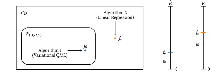
Figure 1: Illustration of the relationship between $\mathcal{F}_{\mathcal{D}}$ and $\mathcal{F}_{(\Theta,\mathcal{D},O)}$, and the output of Algorithms 1 and 2. In particular, we always have that $\mathcal{F}_{(\Theta,\mathcal{D},O)}\subset\mathcal{F}_{\mathcal{D}}$. As a consequence of this, and the fact that Algorithm 2 is a perfect empirical risk minimizer, we always have that $\hat{R}(f_{v})\leq\hat{R}(f_{\theta})$. However, it might be the case that $R(f_{v})\geq R(f_{\theta})$.

Note on recent related work: As per the discussion above, the two motivations for introducing Algorithm 3 were the poor efficiency and potentially poor generalization associated to Algorithm 2. However, we note that in Ref. [STJ23], which appeared recently, the authors show via a tensor network analysis that to every PQC architecture one can associate a feature map – different from the PQC feature map $\phi_{\mathcal{D}}$ – for which (a) all functions in the PQC model class are linear with respect to the feature map, and (b) the associated kernel can be evaluated efficiently classically. As such, using this feature map, for any number of data-samples $n$, one can run Algorithm 2 classically efficiently with respect to $d$ – i.e., there is no need to approximate the kernel via RFF! Indeed, this approach to dequantization is suggested by the authors of Ref. [STJ23]. However as above, and discussed in Ref. [STJ23], this does not immediately yield an efficient dequantization of variational QML, due to the potentially poor generalization of linear regression over the entire function space. In light of this, the generalization of linear regression with respect to the kernel introduced in Ref. [STJ23] certainly deserves attention, and we hope that the methods and tools introduced in this work can be useful in that regard.

4 Generalization and efficiency guarantees for RFF-based linear regression

In this section, we attempt to provide rigorous answers to Question 2 – i.e., for which PQC architectures and for which regression problems does RFF-based linear regression yield an efficient dequantization of variational QML?

In particular, this section is structured as follows: We begin in Section 4.1 with a brief digression, providing definitions for some important kernel notions. With these in hand, we continue in Section 4.2 to state Theorem 1 which provides a concrete answer to Question 2. In particular, Theorem 1 provides an upper bound on both the number of data samples $n$, and the number of frequency samples $M$, which are sufficient to ensure that, with high probability, the output of RFF-based linear regression with respect to the kernel $K_{\mathcal{D}}$ is a good approximation to the best possible PQC function, with respect to true risk. As we will see, these upper bounds depend crucially on two quantities which are defined in Section 4.1, namely the operator norm of the kernel integral operator associated to $K_{\mathcal{D}}$, and the reproducing kernel Hilbert space norm of the optimal PQC function.

Given the results of Section 4.2, in order to make any concrete statements it is necessary to gain a deeper quantitative understanding of both the operator norm of the kernel integral operator and the RKHS norm of functions in the PQC model class. However, before doing this, we show in Section 4.3 that the PQC feature map $\phi_{\mathcal{D}}$ is in fact a special instance of an entire family of feature maps – which we call “re-weighted PQC feature maps” – and that Theorem 1 holds not only for $K_{\mathcal{D}}$, but for the kernel induced by any such re-weighted feature map. With this in hand, we then proceed in Section 4.4 to show how the re-weighting determines the distribution over frequencies $\pi$ from which one needs to sample in the RFF procedure, and we discuss in detail for which feature maps/kernels one can and cannot efficiently sample from this distribution. This immediately allows us to rule out efficient RFF dequantization for a large class of re-weighted PQC feature maps, and therefore allows us to focus our attention on only those feature maps (re-weightings) which admit efficient sampling procedures.

With this knowledge, we then proceed in Sections 4.5 and 4.6 to discuss in detail the quantitative behaviour of the kernel integral operator and the RKHS norm of PQC functions, for different re-weighted PQC kernels. This allows us to place further restrictions on the circuit architectures and re-weightings which yield efficient PQC dequantization via Theorem 1. Finally, in Section 4.7 we show that the properties we have identified in Sections 4.5 and 4.6 as sufficient for the application of Theorem 1 are in some sense necessary. In particular, we prove lower bounds on the number of frequency samples necessary to achieve a certain average error via RFF, and use this to delineate rigorously when efficient dequantization via RFF is not possible.

4.1 Preliminary kernel theory

In order to present Theorem 1 we require a few definitions. To start, we need the notion of a reproducing kernel Hilbert space (RKHS), and the associated RKHS norm.

Definition 2: (RKHS and RKHS norm)

Given a kernel $K\colon\mathcal{X}\times\mathcal{X}\rightarrow\mathbb{R}$ we define the associated reproducing kernel Hilbert space (RKHS) as the tuple $(\mathcal{H}_{K},\langle\cdot,\cdot\rangle_{K})$ where $\mathcal{H}_{K}$ is the set of functions defined as the completion (including limits of Cauchy series) of

$$\mathrm{span}\{K_{x}(\cdot)\coloneqq K(x,\cdot)\,|\,x\in\mathcal{X}\},$$ (37)

and $\langle\cdot,\cdot\rangle_{K}$ is the inner product on $\mathcal{H}_{K}$ defined via

$$\langle g,h\rangle_{\mathcal{H}_{K}}\coloneqq\sum_{i,j}\alpha_{i}\beta_{j}K(x_{i},x_{j})$$ (38)

for any two functions $g=\sum_{i}\alpha_{i}K_{x_{i}}$ and $h=\sum_{j}\beta_{j}K_{x_{j}}$ in $\mathcal{H}_{K}$. This inner product then induces the RKHS norm $\|\cdot\|_{K}$ defined via

$$\|g\|_{K}\coloneqq\sqrt{\langle g,g\rangle_{\mathcal{H}_{K}}}.$$ (39)

It is crucial to note that for two kernels $K_{1}$ and $K_{2}$ it may be the case that $\mathcal{H}_{K_{1}}=\mathcal{H}_{K_{2}}$ but $\|\cdot\|_{K_{1}}\neq\|\cdot\|_{K_{2}}$. We will make heavy use of this fact shortly. In particular, the re-weighted PQC kernels introduced in Section 4.3 have precisely this property. In addition to the definition above, we also need a definition of the kernel integral operator associated to a kernel, which we define below.

Definition 3: (Kernel integral operator)

Given a kernel $K\colon\mathcal{X}\times\mathcal{X}\rightarrow\mathbb{R}$ and a probability distribution $P_{\mathcal{X}}$ over $\mathcal{X}$, we start by defining the space of square-integrable functions with respect to $P_{\mathcal{X}}$ via

$$L^{2}(\mathcal{X},P_{\mathcal{X}})=\left\{f\in\mathbb{R}^{\mathcal{X}}\text{ such that }\int_{\mathcal{X}}|f(x)|^{2}\,\mathrm{d}P_{\mathcal{X}}(x)<\infty\right\}.$$ (40)

The kernel integral operator $T_{K}\colon L^{2}(\mathcal{X},P_{\mathcal{X}})\rightarrow L^{2}(\mathcal{X},P_{\mathcal{X}})$ is then defined via

$$(T_{K}g)(x)=\int_{\mathcal{X}}K(x,x^{\prime})g(x^{\prime})\,\mathrm{d}P_{\mathcal{X}}(x^{\prime})$$ (41)

for all $g\in L^{2}(\mathcal{X},P_{\mathcal{X}})$.

In addition, we note that we will mostly be concerned with the operator norm of the kernel integral operator, which we denote with $\|T_{K}\|$ – i.e., when no subscript is used to specify the norm, we assume the operator norm.

4.2 Efficiency of RFF for matching variational QML

Given the definitions of Section 4.1, we proceed in this section to state Theorem 1, which provides insight into the number of data samples $n$ and the number of frequency samples $M$ which are sufficient to ensure that, with probability at least $1-\delta$, the true risk of the output hypothesis of RFF-based linear regression is no more than $\epsilon$ worse than the true risk of the best possible function realizable by the PQC architecture. To this end, we require first a preliminary definition of the “best possible PQC function”:

Definition 4: (Optimal PQC function)

Given a regression problem $P\sim\mathcal{X}\times\mathbb{R}$, and a PQC architecture $(\Theta,\mathcal{D},O)$, we define $f^{*}_{(\Theta,\mathcal{D},O)}$, the optimal PQC model for $P$ (with respect to true risk), via

$$f^{*}_{(\Theta,\mathcal{D},O)}=\operatorname*{arg\,min}_{f\in\mathcal{F}_{(\Theta,\mathcal{D},O)}}\left[R(f)\right].$$ (42)

With this in hand we can state Theorem 1. We note however that this follows via a straightforward application of the RFF generalization bounds provided in Ref. [RR17] to the PQC-kernel, combined with the insight that the set of PQC functions $\mathcal{F}_{(\Theta,\mathcal{D},O)}$ is contained within the $H_{K_{\mathcal{D}}}$, the RKHS associated with the PQC-kernel. A detailed proof is provided in Appendix B.

Theorem 1: (RFF vs. variational QML)

Let $R$ be the risk associated with a regression problem $P\sim\mathcal{X}\times\mathbb{R}$. Assume the following:

1. $\|f^{*}_{(\Theta,\mathcal{D},O)}\|_{K_{\mathcal{D}}}\leq C$

2. $|y|\leq b$ almost surely when $(x,y)\sim P$, for some $b>0$.

Additionally, define

$$n_{0} \coloneqq\max\left\{4\|T_{K_{\mathcal{D}}}\|^{2},\left(528\log\frac{1112\sqrt{2}}{\delta}\right)^{2}\right\},$$ (43)

$$c_{0} \coloneqq 36\left(3+\frac{2}{\|T_{K_{\mathcal{D}}}\|}\right),$$ (44)

$$c_{1} \coloneqq 8\sqrt{2}(4b+\frac{5}{\sqrt{2}}C+2\sqrt{2C}).$$ (45)

Then, let $\delta\in(0,1]$, let $n\geq n_{0}$, set $\lambda_{n}=1/\sqrt{n}$, and let $\hat{f}_{M_{n},\lambda_{n}}$ be the output of $\lambda_{n}$-regularized linear regression with respect to the feature map

$$\phi_{M_{n}}(x)=\frac{1}{\sqrt{M_{n}}}\big{(}\psi(x,\nu_{1}),\ldots,\psi(x,\nu_{M})\big{)}$$ (46)

constructed from the integral representation of $K_{\mathcal{D}}$ by sampling $M_{n}$ elements from $\pi$. Then, with probability at least $1-\delta$, one achieves either

$$R(\hat{f}_{M_{n},\lambda_{n}})\leq R(f^{*}_{(\Theta,\mathcal{D},O)})$$ (47)

or

$$R(\hat{f}_{M_{n},\lambda_{n}})-R(f^{*}_{(\Theta,\mathcal{D},O)})\leq\epsilon,$$ (48)

by ensuring that

$$n\geq\max\left\{\frac{c_{1}^{2}\log^{4}\frac{1}{\delta}}{\epsilon^{2}},n_{0}\right\}$$ (49)

and

$$M\geq c_{0}\sqrt{n}\log\frac{108\sqrt{n}}{\delta}.$$ (50)

Let us now try to unpack what insights can be gained from Theorem 1. Firstly, recall that here we consider $\mathcal{X}\subseteq\mathbb{R}^{d}$, in which case $d$ provides the relevant asymptotic scaling parameter. With this in mind, in order to gain intuition, assume for now that $n_{0},c_{0}$ and $c_{1}$ are constants with respect to $d$. Assume additionally that one can sample efficiently from $\pi$. In this case we see via Theorem 1 that both the number of data points $n$, and the number of samples $M$, which are sufficient to ensure that with probability $1-\delta$ there is a gap of at most $\epsilon$ between the true risk of PQC optimization and the true risk of RFF, is independent of $d$, and polylogarithmic in both $1/\epsilon$ and $1/\delta$. Given that the time and space complexity of RFF-based linear regression is $\mathcal{O}(nM)$ and $\mathcal{O}(nM^{2}+M^{3})$, respectively, in this case Theorem 1 guarantees that Algorithm 3 (RFF based linear regression) provides an efficient dequantization of variational QML.

However, in general $n_{0},c_{0}$ and $c_{1}$ will not be constants, and one will not be able to sample efficiently from $\pi$. In particular, $n_{0},c_{0}$ and $c_{1}$ depend on both $\|T_{K_{\mathcal{D}}}\|$, the operator norm of the kernel integral operator, and $C$, the upper bound on the RKHS norm of the optimal PQC function. Given the form of $n_{0},c_{0}$ and $c_{1}$, in order for Theorem 1 to yield a polynomial upper bound on $n$ and $M$, it is sufficient that $\|T_{K_{\mathcal{D}}}\|=\Omega(1/\mathrm{poly}(d))$ and that $C=\mathcal{O}(\mathrm{poly}(d))$.

Summary: In order to use Theorem 1 to make any concrete statement concerning the efficiency of RFF for dequantizing variational QML, we need to obtain the following.

1. Lower bounds on $\|T_{K_{\mathcal{D}}}\|$, the operator norm of the kernel integral operator.

2. Upper bounds on $\|f^{*}_{(\Theta,\mathcal{D},O)}\|_{K_{\mathcal{D}}}$, the RKHS norm of the optimal PQC function.

3. An understanding of the complexity of sampling from $\pi$, the distribution appearing in the integral representation of $K_{\mathcal{D}}$.

We address the above requirements in the following sections. However, before doing that, we note in Section 4.3 below that Theorem 1 applies not only to $K_{\mathcal{D}}$, but to an entire family of “re-weighted” kernels, of which $K_{\mathcal{D}}$ is a specific instance. We will see that this is important as different re-weightings will lead to substantially different sampling complexities, as well as lower and upper bounds on $\|T_{K_{\mathcal{D}}}\|$ and $C$, respectively.

4.3 Re-weighted PQC kernels

As mentioned in Section 4.2, the proof of Theorem 1 is essentially a straightforward application of the RFF generalization bound from Ref. [RR17] to the classical PQC kernel $K_{\mathcal{D}}$. However, as discussed in the proof of Theorem 1 in Appendix B, the key insight that allows one to leverage the generalization bound from Ref. [RR17] into a bound on the difference in true risk between the output of variational QML and the output of RFF based linear regression with the PQC kernel $K_{\mathcal{D}}$, is the fact that $\mathcal{F}_{(\Theta,\mathcal{D},O)}$ is a subset of $\mathcal{F}_{\mathcal{D}}$ – i.e., the fact that $\mathcal{F}_{(\Theta,\mathcal{D},O)}\subset\mathcal{F}_{\mathcal{D}}$. With this in mind, here we make the observation that the set $\mathcal{F}_{\mathcal{D}}$, which was defined from the feature map $\phi_{\mathcal{D}}$ and the kernel $K_{\mathcal{D}},$ is in fact invariant under certain re-weightings of the PQC feature map. As a result, Theorem 1 in fact holds not just for $K_{\mathcal{D}}$, but for all of the appropriately re-weighted PQC kernels.

We can now make the notion of a re-weighted PQC kernel precise. For any “re-weighting vector” $w\in\mathbb{R}^{|\Omega_{\mathcal{D}}|}$, we define the re-weighted PQC feature map via

$$\phi_{(\mathcal{D},w)}(x)\coloneqq\frac{1}{\|w\|_{2}}\big{(}w_{0},w_{1}\cos(\langle\omega_{1},x\rangle),w_{1}\sin(\langle\omega_{1},x\rangle),\ldots,w_{|\Omega^{+}_{\mathcal{D}}|}\cos(\langle\omega_{|\Omega^{+}_{\mathcal{D}}|},x\rangle),w_{|\Omega^{+}_{\mathcal{D}}|}\sin(\langle\omega_{|\Omega^{+}_{\mathcal{D}}|},x\rangle)\big{)},$$ (51)

along with the associated set of linear functions with respect to $\phi_{(\mathcal{D},w)}$, defined via

$$\mathcal{F}_{(\mathcal{D},w)}=\{f_{\theta}(\cdot)=\langle v,\phi_{(\mathcal{D},w)}(\cdot)\rangle\,|\,\theta\in\Theta\},$$ (52)

and the associated re-weighted PQC kernel

$$K_{(\mathcal{D},w)}(x,x^{\prime})\coloneqq\langle\phi_{(\mathcal{D},w)}(x),\phi_{(\mathcal{D},w)}(x^{\prime})\rangle.$$ (53)

Note that we recover the previous definitions when $w$ is the vector of all $1$’s (in which case $\|w\|_{2}=\sqrt{|\Omega_{\mathcal{D}}|}$). We can then make the following observation:

Observation 1: (Invariance of $\mathcal{F}_{\mathcal{D}}$ under non-zero feature map re-weighting)

For a re-weighting vector $w\in\mathbb{R}^{|\Omega_{\mathcal{D}}|}$ satisfying $w_{i}\neq 0$ for all $i\in[|\Omega_{\mathcal{D}}|]$, we have that

$$\mathcal{F}_{(\mathcal{D},w)}=\mathcal{F}_{\mathcal{D}}.$$ (54)

Proof.

Define the matrix $M_{w}$ as the matrix with $w$ as its diagonal, and the matrix

$$M\coloneqq\left(\sqrt{|\Omega|_{\mathcal{D}}}/\|w\|_{2}\right)M_{w}.$$ (55)

By the assumptions on $w$, the matrix $M$ is invertible. Now, let $f\in\mathcal{F}_{(\mathcal{D},w)}$. We have that

$$f(\cdot)=\langle v,\phi_{(\mathcal{D},w)}(\cdot)\rangle=\langle v,M\phi_{\mathcal{D}}(\cdot)\rangle=\langle vM,\phi_{\mathcal{D}}(\cdot)\rangle=\langle\tilde{v},\phi_{\mathcal{D}}(\cdot)\rangle,$$ (56)

i.e., $f\in\mathcal{F}_{\mathcal{D}}$, and, therefore, $\mathcal{F}_{(\mathcal{D},w)}\subset\mathcal{F}_{\mathcal{D}}$. Similarly, for all $g\in\mathcal{F}_{\mathcal{D}}$ we have that

$$g(\cdot)=\langle v,\phi_{\mathcal{D}}(\cdot)\rangle=\langle v,M^{-1}M\phi_{\mathcal{D}}(\cdot)\rangle=\langle vM^{-1},M\phi_{\mathcal{D}}(\cdot)\rangle=\langle\tilde{v}|\phi_{(\mathcal{D},w)}(\cdot)\rangle,$$ (57)

i.e., $g\in\mathcal{F}_{(\mathcal{D},w)}$, and hence $\mathcal{F}_{\mathcal{D}}\subset\mathcal{F}_{(\mathcal{D},w)}$. ∎

We note that Observation 1, combined with the fact that $\mathcal{F}_{(\Theta,\mathcal{D},O)}\subset\mathcal{F}_{\mathcal{D}}$, implies that $\mathcal{F}_{(\Theta,\mathcal{D},O)}\subset\mathcal{F}_{(\mathcal{D},w)}$. As alluded to before, we therefore see that Theorem 1 actually holds for any PQC kernel $K_{(\mathcal{D},w)}$, re-weighted via a re-weighting vector $w$ with no zero elements. We note that allowing re-weighting vectors with zero elements has the effect of “shrinking” the set $F_{(\mathcal{D},w)}$, which might result in the existence of functions $f$ satisfying both $f\in\mathcal{F}_{(\Theta,\mathcal{D},O)}$ and $f\notin F_{(\mathcal{D},w)}$. Intuitively, this is problematic because for regression problems in which $f$ is the optimal solution, we know that the PQC architecture $(\Theta,\mathcal{D},O)$ can realize $f$, but we cannot hope for the RFF procedure $K_{(\mathcal{D},w)}$ to do the same, as it is limited to hypotheses within $F_{(\mathcal{D},w)}$.

In light of the above observations, from this point on we can broaden our discussion of the application of Theorem 1 to include all appropriately re-weighted PQC kernels. This insight is important because:

1. We will see that all appropriately re-weighted PQC kernels give rise to the same function set $\mathcal{F}_{\mathcal{D}}$, but to different RKHS norms. As a result, the RKHS norm of the optimal PQC function – which as we have seen is critical to the complexity of the RFF method – will depend on which re-weighting we choose.

2. Similarly, we will see that the operator norm of the kernel integral operator – and therefore again the complexity of RFF linear regression – depends heavily on the re-weighting chosen.

3. We will see that the re-weighting of the PQC kernel completely determines the probability distribution $\pi$, from which it is necessary to sample in order to implement RFF-based linear regression. Therefore, once again, the efficiency of RFF will depend on the re-weighting chosen. This perspective will also allow us to see why zero elements are not allowed in the re-weighting vector. Namely, because doing this will cause the probability of sampling the associated frequency to be zero, which is problematic if that frequency is required to represent the regression function.

4.4 RFF implementation

Recall from Section 2.3, and from our presentation of Algorithm 3 in Section 3, that when given a shift-invariant kernel $K$, in order to implement RFF-based linear regression, one has to sample from the probability measure $\pi=p\times\mu$, which one obtains from the Fourier transform of $K$. As such, given a re-weighted PQC kernel $K_{(\mathcal{D},w)}$, we need to:

1. Understand the structure of the probability distribution $p$, which should depend on both $\mathcal{D}$ and the re-weighting vector $w$.

2. Understand when and how – i.e., for which data-encoding strategies and which re-weightings – one can efficiently sample from $p$.

Let us begin with point 1. To this end we start by noting that the re-weighted PQC kernels $K_{(\mathcal{D},w)}$ have a particularly simple integral representation, from which one can read off the required distribution. In particular, note that

$$K_{(\mathcal{D},w)}(x,x^{\prime}) =\langle\phi_{(\mathcal{D},w)}(x),\phi_{(\mathcal{D},w)}(x^{\prime})\rangle$$ (58)

$$=\frac{1}{\|w\|^{2}_{2}}\left(w_{0}^{2}+\sum_{i=1}^{|\Omega^{+}_{\mathcal{D}}|}w_{i}^{2}\left[\cos(\langle\omega_{i},x\rangle)\cos(\langle\omega_{i},x^{\prime}\rangle)+\sin(\langle\omega_{i},x\rangle)\sin(\langle\omega_{i},x^{\prime}\rangle)\right]\right)$$ (59)

$$=\frac{1}{\|w\|^{2}_{2}}\sum_{i=0}^{|\Omega^{+}_{\mathcal{D}}|}w_{i}^{2}\left[\cos(\langle\omega_{i},x\rangle)\cos(\langle\omega_{i},x^{\prime}\rangle)+\sin(\langle\omega_{i},x\rangle)\sin(\langle\omega_{i},x^{\prime}\rangle)\right]$$ (60)

$$=\frac{1}{\|w\|^{2}_{2}}\sum_{i=0}^{|\Omega^{+}_{\mathcal{D}}|}w_{i}^{2}\left[\cos(\langle\omega_{i},(x-x^{\prime})\rangle)\right],$$ (61)

$$=\frac{1}{2\pi}\int_{\mathcal{X}}\int_{0}^{2\pi}\sqrt{2}\cos(\langle\omega,x\rangle+\gamma)\sqrt{2}\cos(\langle\omega,x^{\prime}\rangle+\gamma)q_{(\mathcal{D},w)}(\omega)\,\,\mathrm{d}\gamma\mathrm{d}\nu,$$ (62)

where

$$q_{(\mathcal{D},w)}(\omega)=\sum_{i=0}^{|\Omega^{+}_{\mathcal{D}}|}\frac{w_{i}^{2}}{\|w\|^{2}_{2}}\delta(\omega-\omega_{i}),$$ (63)

and $\delta$ is the Dirac delta function. By comparison with Eq. (14) we therefore see that $\pi=q_{(\mathcal{D},w)}\times\mu$, where as before, $\mu$ is the uniform distribution over $[0,2\pi)$. For convenience, we refer to $q_{(\mathcal{D},w)}$ as the probability distribution associated to $K_{(\mathcal{D},w)}$.

Let us now move on to point 2 – in particular, for which data encoding strategies and re-weighting vectors can we efficiently sample from $q_{(\mathcal{D},w)}$? Firstly, note that sampling from the continuous distribution $q_{(\mathcal{D},w)}$ can be done by sampling from the discrete distribution $p_{(\mathcal{D},w)}$ over $\Omega_{\mathcal{D}}$ defined via

$$p_{(\mathcal{D},w)}(\omega_{i})=\frac{w_{i}^{2}}{\|w\|^{2}_{2}}$$ (64)

for all $\omega_{i}\in\Omega_{\mathcal{D}}$. As a result, from this point on we focus on the distribution $p_{(\mathcal{D},w)}$, and when clear from the context we drop the subscript and just use $p$ to refer to $p_{(\mathcal{D},w)}$. Also, we note that we can in principle just work directly with the choice of probability distribution, as opposed to the underlying weight vector, as we know for any probability distribution over $\Omega_{\mathcal{D}}$ there exists an appropriate weight vector.

As $p$ is a distribution over $\Omega_{\mathcal{D}}$, in order to discuss the efficiency of sampling from $p$, it is necessary to briefly recall some facts about the sets $\Omega_{\mathcal{D}}$ and $\tilde{\Omega}_{\mathcal{D}}$. In particular, as discussed in Appendix A, given a data-encoding strategy $\mathcal{D}=\left(\mathcal{D}^{(1)},\ldots,\mathcal{D}^{(d)}\right)$, where $\mathcal{D}^{(j)}$ contains the Hamiltonians used to encode the $j$’th data component $x_{j}$, we know that

$$\tilde{\Omega}_{\mathcal{D}}=\tilde{\Omega}^{(1)}_{\mathcal{D}}\times\ldots\times\tilde{\Omega}^{(d)}_{\mathcal{D}},$$ (65)

where $\tilde{\Omega}^{(j)}_{\mathcal{D}}\subset\mathbb{R}$ depends only on $\mathcal{D}^{(j)}$ – i.e., $\tilde{\Omega}_{\mathcal{D}}$ has a Cartesian product structure. Additionally, as discussed in Section 2.4 we know that $\tilde{\Omega}_{\mathcal{D}}\coloneqq\Omega_{\mathcal{D}}\cup\left(-\Omega_{\mathcal{D}}\right)$, where $\Omega_{\mathcal{D}}\cap\left(-\Omega_{\mathcal{D}}\right)=\{\omega_{0}\}$. Taken together, we see that

$$|\tilde{\Omega}_{\mathcal{D}}| =\prod_{j=1}^{d}|\tilde{\Omega}_{\mathcal{D}}^{(j)}|,$$ (66)

$$|\Omega_{\mathcal{D}}| =\frac{|\tilde{\Omega}_{\mathcal{D}}|-1}{2}+1.$$ (67)

Now, let us define $N_{j}:=|\tilde{\Omega}^{(j)}_{\mathcal{D}}|$, and make the assumption that $N_{j}$ is independent of $d$. Furthermore, let us define $N_{\text{min}}=\min\{N_{j}\}$. We then have that

$$|\tilde{\Omega}_{\mathcal{D}}|\geq N_{\text{min}}^{d}$$ (68)

i.e., that the number of frequencies in $\tilde{\Omega}_{\mathcal{D}}$, and therefore $\Omega_{\mathcal{D}}$, scales exponentially with respect to $d$. From this we can immediately make our first observation:

Observation 2:

Given that the number of elements in $\Omega_{\mathcal{D}}$ scales exponentially with $d$, one cannot efficiently store and sample from arbitrary distributions supported on $\Omega_{\mathcal{D}}$.

As such, we have to restrict ourselves to structured distributions, whose structure facilitates efficient sampling. One such subset of distributions are those which are supported only on a polynomial (in $d$) size subset of $\Omega_{\mathcal{D}}$. Another suitable set of distributions is what we call product-induced distributions. Specifically, let $\tilde{p}^{(j)}$ be an arbitrary distribution over $\tilde{\Omega}^{(j)}_{\mathcal{D}}$, and define the product distribution $\tilde{p}$ over $\tilde{\Omega}_{\mathcal{D}}$ via

$$\tilde{p}\big{(}\omega=(\omega_{1},\ldots,\omega_{d})\big{)}=\tilde{p}^{(1)}(\omega_{1})\times\ldots\times\tilde{p}^{(d)}(\omega_{d}).$$ (69)

Note that, due to the $d$-independence of $|\tilde{\Omega}^{(j)}_{\mathcal{D}}|$ we can store and sample from $\tilde{p}^{(j)}$ efficiently, which then allows us to sample from $\tilde{p}$ by simply drawing $\omega_{j}\sim\tilde{p}^{(j)}$ for all $j\in[d]$ and then outputting $\omega=(\omega_{1},\ldots,\omega_{d})$. However, it may be the case that $\omega\notin\Omega_{\mathcal{D}}$. As such, the natural thing to do is simply output $\omega$ if $\omega\in\Omega_{\mathcal{D}}$, and if not, output $-\omega$. If one does this, then one samples from the distribution $p$ over $\Omega_{\mathcal{D}}$ defined via

$$p(\omega):=\begin{cases}\tilde{p}(\omega)\hskip 50.00008pt\text{ if }\omega=\omega_{0},\\ \tilde{p}(\omega)+\tilde{p}(-\omega)\hskip 11.99998pt\text{ else,}\end{cases}$$ (70)

which we refer to as a product-induced distribution. We can in fact however go further, and use the Cartesian product structure of $\tilde{\Omega}_{\mathcal{D}}$ to generalize product-induced distributions to matrix-product-state-induced (MPS-induced) distributions. To do this, let us label the elements of $\tilde{\Omega}^{(j)}_{\mathcal{D}}$ via $\tilde{\Omega}^{(j)}_{\mathcal{D}}=\{\tilde{\Omega}^{(j)}_{k_{j}}\}$ for $k_{j}\in[N_{j}]$. We can then write any $\omega\in\tilde{\Omega}_{\mathcal{D}}$ via $\omega=(\omega^{(1)}_{k_{1}},\ldots,\omega^{(d)}_{k_{d}})$, for some indexing $(k_{1},\ldots,k_{d})$. From this, we see that any distribution $\tilde{p}$ over $\tilde{\Omega}_{\mathcal{D}}$ can be naturally represented as a $d$-tensor - i.e., as as a tensor with $d$ legs, where the $j$’th leg is $N_{j}$ dimensional. Graphically, we have that

$$\tilde{p}[(\omega^{(1)}_{k_{1}},\ldots,\omega^{(d)}_{k_{d}})]=\vbox{\hbox{\includegraphics[height=43.36464pt]{figures/p_tensor.pdf}}}$$ (71)

Now we can consider the subset of distributions which can be represented by a matrix product state [Sch11], i.e., those distributions for which

$$\tilde{p}[(\omega^{(1)}_{k_{1}},\ldots,\omega^{(d)}_{k_{d}})]=\vbox{\hbox{\includegraphics[height=47.69846pt]{figures/p_mps.pdf}}}$$ (72)

We refer to distributions which admit such a representation as MPS distributions [FV12, SW10, pac, GSP+19]. One can efficiently store such distributions whenever the bond dimension $\chi$ is polynomial in $d$, and as described in Refs. [FV12, SW10, pac], one can sample from such distributions with complexity $dN_{\text{max}}\chi^{3}$. Note that the product distribution in Eq. (69) is a special case of an MPS distribution,with $\chi=1$. Now, given an MPS distribution $\tilde{p}$ over $\tilde{\Omega}_{\mathcal{D}}$, we define the induced distribution over $\Omega_{\mathcal{D}}$ via Eq. (70).

Summary: In order to efficiently implement the RFF procedure for a kernel $K_{(\mathcal{D},w)}$, it is necessary that one can sample efficiently from $p_{(\mathcal{D},w)}$, the discrete probability distribution associated to the kernel. However, the number of frequency vectors $|\Omega_{\mathcal{D}}|$ typically scales exponentially in $d$, and as such one cannot efficiently store and sample from arbitrary probability distributions over $\Omega_{\mathcal{D}}$. As such, efficiently implementing RFF is only possible for the subset of kernels whose associated distributions have a structure which facilitates efficient sampling. Due to the Cartesian product structure of $\tilde{\Omega}_{\mathcal{D}}$ one such set of distributions (amongst others) are those induced by MPS with polynomial bond dimension.

4.5 Kernel integral operator for PQC kernels

Recall from Theorem 1 that

$$M\geq c_{o}\sqrt{n}\log\frac{108\sqrt{n}}{\delta}$$ (73)

frequency samples are sufficient to guarantee, with probability greater than $1-\delta$, an error of at most $\epsilon$ between the output of the RFF procedure and the optimal PQC model. As such, in order to fully understand the complexity of RFF-based regression, it is necessary for us to gain a better understanding of $c_{0}$, which is given by

$$c_{0}=9\left(\frac{29}{4}+\frac{4}{\|T_{K_{(\mathcal{D},w)}}\|}\right).$$ (74)

In particular, in order to find the smallest number of sufficient frequency samples, it is necessary for us to obtain an upper bound on $c_{0}$, which in turn requires a lower bound on $\|T_{K_{(\mathcal{D},w)}}\|$, the operator norm of the kernel integral operator associated with $K_{(\mathcal{D},w)}$. We achieve this with the following lemma, whose proof can be found in Appendix C.

Lemma 1: (Operator norm of $T_{(K_{\mathcal{D}},w)}$)

Let $K_{(\mathcal{D},w)}$ be the re-weighted PQC kernel defined via Eq. (53), and let $T_{K_{(\mathcal{D},w)}}$ be the associated kernel integral operator (as per Definition 3). Assume that (a) the marginal distribution $P_{\mathcal{X}}$ appearing in the definition of the kernel integral operator is fixed to the uniform distribution, and (b) The frequency set $\Omega_{\mathcal{D}}$ consists only of integer vectors – i.e., $\Omega_{\mathcal{D}}\subset\mathbb{Z}^{d}$. Then, we have that

$$\|T_{K_{(\mathcal{D},w)}}\| =\max_{i\in|\Omega_{\mathcal{D}}|}\left\{\frac{1}{2}\frac{w_{i}^{2}}{\|w\|^{2}_{2}}\right\}$$ (75)

$$=\max_{\omega\in\Omega_{\mathcal{D}}}\left\{\frac{1}{2}p_{(\mathcal{D},w)}(\omega)\right\}.$$ (76)

In light of this, let us again drop the subscript for convenience, and define $p_{\text{max}}\coloneqq\max_{\omega\in\Omega_{\mathcal{D}}}\left\{p_{(\mathcal{D},w)}(\omega)\right\}$. With this in hand we can immediately make the following observation:

Observation 3:

In order to achieve $c_{0}=\mathcal{O}\left(\mathrm{poly}(d)\right)$, which is necessary for Theorem 1 to imply that ${M=\mathcal{O}(\mathrm{poly}(d))}$ frequency samples are sufficient, we require that

$$p_{\text{max}}=\Omega\left(\frac{1}{\mathrm{poly}(d)}\right),$$ (77)

i.e., the maximum probability of the probability distribution associated to $K_{(\mathcal{D},w)}$ must decay at most inversely polynomially in $d$.

It is important to stress that we have not yet established the necessity that $p_{\text{max}}$ decays inversely polynomially for the RFF procedure to be efficient. In particular, we have only established that this is required for the guarantee of Theorem 1 to be meaningful. However, we will show shortly, in Section 4.7, that Eq. (77) is indeed also necessary, at least in order to obtain a small average error.

In light of Observation 3, we can immediately rule out the meaningful applicability of Theorem 1 for kernels with the following associated distributions:

The uniform distribution: As discussed in Section 4.4, we have that $|\tilde{\Omega}_{\mathcal{D}}|\geq N_{\text{min}}^{d}$, and therefore, for the uniform distribution over $|\Omega_{\mathcal{D}}|$ one has that

$$p_{\text{max}}\leq\frac{2}{N_{\text{min}}^{d}},$$ (78)

i.e., $p_{\mathrm{max}}$ scales inverse exponentially with $d$.

Product-induced distributions: Consider a probability distribution $p$ over $\Omega_{\mathcal{D}}$ induced by the product distribution $\tilde{p}$ over $\tilde{\Omega}_{\mathcal{D}}$, defined as per Eq. (69). We have that

$$p_{\text{max}} \leq 2\tilde{p}_{\text{max}}\hskip 50.00008pt\text{[via Eq.~{}\eqref{eq:induced_distributions}]}$$ (79)

$$=2\prod_{j\in[d]}\tilde{p}^{j}_{\text{max}}\hskip 31.0001pt\text{[via Eq.~{}\eqref{eq:product}]}$$ (80)

$$\leq 2\left(\max_{j\in[d]}\left\{\tilde{p}^{j}_{\text{max}}\right\}\right)^{d}.$$ (81)

Therefore, whenever $\max_{j\in[d]}\left\{\tilde{p}^{j}_{\text{max}}\right\}<1$, there exists some constant $c>1$ such that

$$p_{\text{max}}\leq\frac{2}{c^{d}}.$$ (82)

Summary: In order for Theorem 1 to be meaningfully applicable – i.e to guarantee the efficiency of RFF for approximating variational QML – one requires that the operator norm of the kernel integral operator decays at most inverse polynomially with respect to $d$, which via Lemma 1 requires that the maximum probability of the distribution associated with the kernel decays at most inversely polynomially with $d$. Unfortunately, this rules out any efficiency guarantee, via Theorem 1, for kernels $K_{(\mathcal{D},w)}$ whose associated distribution $p_{(\mathcal{D},w)}$ is either the uniform distribution or a product-induced distribution (with all component probability distributions non-trivial).

4.6 RKHS norm for PQC kernels

Recall from Theorem 1 that one requires

$$n\geq\max\left\{\frac{c_{1}^{2}\log^{4}\frac{1}{\delta}}{\epsilon^{2}},n_{0}\right\}$$ (83)

data samples, in order for Theorem 1 to guarantee, with probability greater than $1-\delta$, an error of at most $\epsilon$ between the output of the RFF procedure and the optimal PQC model. As such, in order to fully understand the complexity of RFF-based regression, it is necessary for us to gain a better understanding of $c_{1}$, which is given by

$$c_{1}\leq 8(4b+3C+2\sqrt{C}),$$ (84)

where $b$ is set by the regression problem (and we can assume to be constant), and $C$ is an upper bound on the RKHS norm of the optimal PQC model, with respect to the kernel used for RFF – i.e.,

$$\|f^{*}_{(\Theta,\mathcal{D},O)}\|_{K_{(\mathcal{D},w)}}\leq C.$$ (85)

Therefore, we see that in order to determine the smallest number of sufficient data samples, it is necessary for us to obtain a concrete upper bound on the RKHS norm of the optimal PQC function with respect to the kernel $K_{(\mathcal{D},w)}$. More specifically, we would like to understand, for which PQC architectures, and for which kernels, one obtains

$$C=\mathcal{O}\left(\mathrm{poly}(d)\right)$$ (86)

as for any such kernel and architecture, we can guarantee, via Theorem 1, the sample efficiency of the RFF procedure for approximating the optimal PQC model.

Ideally we would like to obtain results and insights which are problem independent and therefore we focus here not on the optimal PQC function (which requires knowing the solution to the problem) but on the maximum RKHS norm over the entire PQC architecture. More specifically, given an architecture $(\Theta,\mathcal{D},O)$ we would like to place upper bounds on

$$C_{(\Theta,\mathcal{D},O)}:=\max\left\{\|f\|_{K_{(\mathcal{D},w)}}\,|\,f\in\mathcal{F}_{(\Theta,\mathcal{D},O)}\right\},$$ (87)

as this clearly provides an upper bound on $\|f^{*}_{(\Theta,\mathcal{D},O)}\|_{K_{(\mathcal{D},w)}}$ for any regression problem.

We start off with an alternative definition of the RKHS norm, which turns out to be much more convenient to work with than the one we have previously encountered.

Lemma 2: (Alternative definition of RKHS norm – Adapted from Theorem 4.21 in Ref. [SC08])

Given some kernel $K\colon\mathcal{X}\times\mathcal{X}\rightarrow\mathbb{R}$ defined via

$$K(x,x^{\prime})=\langle\phi(x),\phi(x^{\prime})\rangle,$$ (88)

for some feature map $\phi\colon\mathcal{X}\rightarrow\mathcal{X}^{\prime}$, one has that

$$\|f\|_{K}=\inf\,\{\|v\|_{2}\,|\,v\in\mathcal{X}^{\prime}\text{ such that }f(\cdot)=\langle v,\phi(\cdot)\rangle\}$$ (89)

for all $f\in\mathcal{H}_{K}$.

In words, Lemma 2 says that the RKHS norm is defined as the infimum over the 2-norms of all hyperplanes in feature space which realize $f$ - i.e., the infimum over $\|v\|_{2}$ for all $v$ such that $f(x)=\langle v,\phi(x)\rangle$. We stress that in general functions in the reproducing kernel Hilbert space do not have a unique hyper-plane representation with respect to the feature map. However, as detailed in Observation 4 below, for PQC feature maps and data-encoding strategies giving rise to integer frequency vectors (such as encoding strategies using only Pauli Hamiltonians [SSM21]), the hyperplane representation is indeed unique.

Observation 4: (Hyperplane uniqueness for integer frequencies)

Let $\mathcal{D}$ be an encoding strategy for which ${\Omega^{+}_{\mathcal{D}}\subset\mathbb{Z}^{d}}$. In this case, one has that

$$\left\{1,\cos(\langle\omega_{1},x\rangle),\sin(\langle\omega_{1}x\rangle),\ldots,\cos(\langle\omega_{|\Omega^{+}_{\mathcal{D}}|},x\rangle),\sin(\langle\omega_{|\Omega^{+}_{\mathcal{D}}|},x\rangle)\right\}$$ (90)

is a mutually orthogonal set of functions. Therefore for any strictly positive re-weighting $w$, and any $u,v\in\mathbb{R}^{|\tilde{\Omega}_{\mathcal{D}}|}$, if ${f(\cdot)=\langle v,\phi_{(\mathcal{D},w)}(\cdot)\rangle}$ and $f(\cdot)=\langle u,\phi_{(\mathcal{D},w)}(\cdot)\rangle$ then $u=v$. Specifically, there exists only one hyperplane in feature space which realizes $f$. As a consequence one has, via Lemma 2, that if $f(\cdot)=\langle v,\phi_{(\mathcal{D},w)}(\cdot)\rangle$ then

$$\|f\|_{K_{(\mathcal{D},w)}}=\|v\|_{2}.$$ (91)

With this in hand, we can do some examples to gain intuition into the behaviour of the RKHS norm.

Example 1:

Given a data-encoding strategy $\mathcal{D}$, and the uniform weight vector $w=\frac{1}{\sqrt{|\Omega_{\mathcal{D}}|}}(1,\ldots,1)$, consider the function $f(x)=\cos(\langle\omega_{1},x\rangle)$. In this case one has that $f(\cdot)=\langle v,\phi_{(\mathcal{D},w)}(\cdot)\rangle$ with

$$v=\left(0,\sqrt{|\Omega_{\mathcal{D}}|},0,\ldots,0\right),$$ (92)

and therefore $\|f\|_{K_{(\mathcal{D},w)}}\leq\sqrt{|\Omega_{\mathcal{D}}|}$, with an equality in the case of encoding strategies with integer frequency vectors. Note that we obtain the same result for $f(x)=\cos(\langle\omega,x\rangle)$ and $f(x)=\sin(\langle\omega,x\rangle)$ for any $\omega\in\Omega_{\mathcal{D}}$.

Example 2:

Let us consider the same function as in Example 1 – i.e., $f(x)=\cos(\langle\omega_{1},x\rangle)$ – but this time let us consider the weight vector $w=(0,1,0,\ldots,0)$. In this case one has $f(\cdot)=\langle v,\phi_{(\mathcal{D},w)}(\cdot)\rangle$ with

$$v=\left(0,1,0\ldots,0\right),$$ (93)

and therefore $\|f\|_{K_{(\mathcal{D},w)}}\leq 1$, with an equality in the case of encoding strategies with integer frequency vectors. We again get the same result for $f(x)=\cos(\langle\omega,x\rangle)$ and $f(x)=\sin(\langle\omega,x\rangle)$ for any $\omega\in\Omega_{\mathcal{D}}$, if one uses the weight vector with $w_{\omega}=1$.

Example 3:

Given a data-encoding strategy $\mathcal{D}$, and the uniform weight vector $w=\frac{1}{\sqrt{|\Omega_{\mathcal{D}}|}}(1,\ldots,1)$, consider the function

$$f(x)=\frac{1}{|\Omega_{\mathcal{D}}|}\sum_{\omega\in\Omega_{\mathcal{D}}}\cos(\langle\omega,x\rangle).$$ (94)

In this case one has $f(\cdot)=\langle v,\phi_{(\mathcal{D},w)}(\cdot)\rangle$ with

$$v=\frac{1}{\sqrt{|\Omega_{\mathcal{D}}|}}\left(1,1,0,1,0\ldots,1,0\right),$$ (95)

and therefore $\|f\|_{K_{(\mathcal{D},w)}}\leq 1$, with an equality in the case of encoding strategies with integer frequency vectors.

Given these examples, we can extract the following important observations:

1. As per Example 1, there exist functions, and re-weighted PQC kernels, for which the RKHS norm of the function scales with the number of frequencies in $\Omega_{\mathcal{D}}$, and therefore exponentially in $d$. As such, we cannot hope to place a universally applicable (architecture independent) polynomial (in $d$) upper bound on $C_{(\Theta,\mathcal{D},O)}$. On the contrary, as per Examples 2 and 3 there do exist functions and reweightings for which the RKHS norm is constant. Therefore, while we cannot hope to place an architecture independent upper bound on the RKHS norm, it may be the case that there exist specific circuit architectures and kernel re-weightings for which $C_{(\Theta,\mathcal{D},O)}$ is upper bounded by a polynomial in $d$. Note that this can be interpreted as an expressivity constraint on $(\Theta,\mathcal{D},O)$, as the more expressive an architecture is, the more likely it contains a function with large RKHS norm (with this likelihood becoming a certainty for the case of universal architectures).

2. By comparing Examples 1 and 2 we see that, as expected, the RKHS norm of a function depends strongly on the reweighting which defines the kernel. In particular, the same function can have a very different RKHS norm with respect to different feature map re-weightings.

3. By looking at all examples together, we see that informally, what seems to determine the RKHS norm of a given function $f_{v}$ is the “alignment” between (a) the frequency distribution of the function $f_{v}$, i.e., the components of the vector $v$, and (b) the re-weighting vector $w$ (or alternatively, the probability distribution $p_{(\mathcal{D},\omega)}$). In particular, in Example 1, the frequency representation of the function $f$ is peaked on a single frequency, whereas the probability distribution $p_{(\mathcal{D},\omega)}$ is uniform over all frequencies. In this example, $v$ and $p_{(\mathcal{D},\omega)}$ are non-aligned, and we find that the RKHS norm of $f$ with respect to $K_{(\mathcal{D},\omega)}$ scales exponentially in $D$. On the contrary, in both Examples 2 and 3 we have that the frequency representation of $f$ is well aligned with the probability distribution $p$, and we find that we can place a constant upper bound on the RKHS norm of the function.

4. At an intuitive level, one should expect the “alignment” between the frequency representation of a target function and the probability distribution associated with the kernel to play a role in the complexity of RFF. Informally, in order to learn an approximation of the function $f_{v}$ via RFF, when constructing the approximate kernel via frequency sampling we need to sample frequencies present in $v$. Therefore, if the distribution is supported mainly on frequencies not present in $v$, we cannot hope to achieve a good approximation via RFF. On the contrary, if the distribution is supported on frequencies present in $v$, with the correct weighting, then we can hope to approximate $f_{v}$ using our approximate kernel. In this sense, our informal observation that the RKHS norm depends on the alignment of target function with kernel probability distribution squares well with our intuitive understanding of RFF-based linear regression. We will make this intuition much more precise in Section 4.7.

Summary: In order for the statement of Theorem 1 to imply that a polynomial number of data samples is sufficient, we require that $\|f^{*}_{(\Theta,\mathcal{D},O)}\|_{K_{(\mathcal{D},w)}}$, the RKHS norm of the optimal PQC function, scales polynomially with respect to $d$. Unfortunately, in the worst case, $\|f^{*}_{(\Theta,\mathcal{D},O)}\|_{K_{(\mathcal{D},w)}}$ can scale exponentially with respect to $d$, and therefore we cannot hope for efficient dequantization of variational QML via RFF for all possible circuit architectures. However, given a specific circuit architecture, and a re-weighting which leads to a distribution $p_{(\mathcal{D},w)}$ with an efficient sampling algorithm, it may be the case that $C_{(\Theta,\mathcal{D},O)}$ scales polynomially in $d$, in which case Theorem 1 yields a meaningful sample complexity for the RFF dequantization of optimization of $(\Theta,\mathcal{D},O)$ for any regression problem $P$. Unfortunately however, it seems unlikely that an expressive circuit architecture will not contain any functions with large RKHS norm. Ultimately though, all that is required by Theorem 1 is that the RKHS norm of the optimal PQC function scales polynomially in $d$, and this may be the case even when $C_{(\Theta,\mathcal{D},O)}$ scales superpolynomially. Unfortunately, given a regression problem $P$ it is not clear how to assess the RKHS norm of the optimal PQC function without knowing this function in advance, which seems to require running the PQC optimization.

4.7 Lower bounds for RFF efficiency

By this point we have seen that the following is sufficient for Theorem 1 to imply the efficient dequantization of variational QML via RFF-based linear regression:

1. We need to be able to efficiently sample from $p_{(\mathcal{D},w)}$.

2. The distribution $p_{(\mathcal{D},w)}$ needs to be sufficiently concentrated. In particular, we need $p_{\text{max}}=\Omega(1/\mathrm{poly}(d))$ in order to place a sufficiently strong lower bound on the operator norm of the kernel integral operator.

3. The frequency representation of the optimal PQC function needs to be “well aligned” with the probability distribution $p_{(\mathcal{D},w)}$. This is required to ensure a sufficiently strong upper bound on the RKHS norm of the optimal PQC function.

It is clear that point 1 above is a necessary criterion for efficient dequantization via RFF. However, it is less clear to which extent points 2 and 3 are necessary. In particular, it could be the case that the bounds provided by Theorem 1 are not tight, and that efficient PQC dequantization via RFF is possible even when not guaranteed by Theorem 1. In this section we address this issue, by proving lower bounds on the complexity of RFF, which show that both points 2 and 3 are also necessary conditions, at least in order to obtain an average-case guarantee on the output of RFF with respect to the $L^{2}$-norm.

We consider a data encoding strategy, giving rise to a frequency set $\tilde{\Omega}_{\mathcal{D}}$, as well as a weight vector $w$, giving rise to the sampling distribution $p_{(\mathcal{D},w)}$, which we abbreviate as $p$. Now, given a regression problem, we define the following notions:

1. Let $f^{*}_{(\Theta,\mathcal{D},O)}$ represent the optimal PQC model. In this section, for convenience we abbreviate this as $f^{*}$.

2. As per Section 2.3 and the description of Algorithm 3 in Section 3, we consider running RFF regression by sampling $M$ frequencies from the distribution $\pi=p\times\mu$. Let $\vec{\omega}=(\omega_{1},\ldots,\omega_{M})\in\Omega^{M}_{\mathcal{D}}$ be the random variable of $M$ frequencies sampled from $p$, and let $g_{\vec{\omega}}$ be the output of linear regression using these frequencies to approximate the kernel $K_{(\mathcal{D},w)}$.

In this section, we are concerned with lower bounding the expected $L^{2}$-norm of the difference between the optimal PQC function and the output of the RFF procedure, with respect to multiple runs of RFF-based linear regression. In particular, we want to place lower bounds on the quantity

$$\hat{\epsilon}\coloneqq \underset{\vec{\omega}\sim p^{M}}{\mathbb{E}}\|f^{*}-g_{\vec{\omega}}\|^{2}_{2}$$ (96)

$$= \sum_{\vec{\omega}\in\Omega^{M}_{\mathcal{D}}}\|f^{*}-g_{\vec{\omega}}\|_{2}^{2}\xi(\vec{\omega})$$ (97)

where $\xi=p^{M}$, i.e., $\xi(\vec{\omega})=p(\omega_{1})\times\ldots\times p(\omega_{M})$. In order to lower bound $\hat{\epsilon}$, recall from Section 2.4 that $f^{*}$ can be written as

$$f^{*}(x)=\sum_{\omega\in\tilde{\Omega}_{\mathcal{D}}}\hat{f}^{*}(\omega)e^{i\langle\omega,x\rangle}.$$ (98)

We abuse notation slightly and use the notation $\hat{f}^{*}$ to denote the vector with entries $\hat{f}^{*}(\omega)$. Finally, we denote by $p_{\text{max}}$ the maximum probability in $p$. With this in hand, we have the following lemma (whose proof can be found in Appendix D):

Lemma 3: (Lower bound on average relative error)

The expected $L^{2}$-norm of the difference between the optimal PQC function and the output of RFF-based linear regression can be lower bounded as

$$\hat{\epsilon} \geq(2\pi)^{d}\|\hat{f}^{*}\|_{2}^{2}-(2\pi)^{d}2M\sum_{\omega\in\Omega_{\mathcal{D}}}|\hat{f}^{*}(\omega)|^{2}p(\omega)$$ (99)

$$\geq(2\pi)^{d}\|\hat{f}^{*}\|_{2}^{2}-(2\pi)^{d}2M\sum_{\omega\in\Omega_{\mathcal{D}}}|\hat{f}^{*}(\omega)|^{2}p_{\max}$$ (100)

$$=\|f^{*}\|_{2}^{2}\left(1-2Mp_{\max}\right).$$ (101)

Using this Lemma, we can now see that indeed both concentration of the probability distribution $p$, and “alignment” of the frequency representation of the optimal function with $p$, are necessary conditions to achieve a small expected relative error $\hat{\epsilon}$.

Concentration of $p$: To this end, note that we can rewrite Eq. (101) as

$$M\geq\frac{1}{2p_{\text{max}}}\left(1-\frac{\hat{\epsilon}}{\|f^{*}\|_{2}^{2}}\right).$$ (102)

Therefore, provided $\hat{\epsilon}/\|f^{*}\|_{2}^{2}$ is asymptotically upper bounded by some constant less than 1 (which, for example, will be the case for constant $\hat{\epsilon}$ and growing $\|f^{*}\|_{2}^{2}$), then one requires ${M=\Omega(1/p_{\text{max}})}$ frequency samples to achieve expected relative error $\hat{\epsilon}$. Given this, we see that the RFF procedure cannot be efficient whenever $p_{\text{max}}$ is a negligible function – i.e., decays faster than any inverse polynomial. Recall from Section 4.5 that for all product-induced distributions, including the uniform distribution, $p_{\text{max}}$ is a negligible function of $d$ - and therefore we cannot achieve efficient RFF dequantization of variational QML via any re-weighting giving rise to such a distribution. However, on the contrary, as also discussed in Section 4.5, whenever $p_{\text{max}}=\Omega(1/\mathrm{poly}(d))$ then one can apply Theorem 1 to place a polynomial upper bound on $M$.

Alignment of $\hat{f}^{*}$ and $p$: Note that we can rewrite Eq. (99) as

$$M\geq\frac{1}{2\sum_{\omega\in\Omega_{\mathcal{D}}}|\hat{f}^{*}(\omega)|^{2}p(\omega)}\left(\|\hat{f}^{*}\|^{2}_{2}-\frac{\hat{\epsilon}}{(2\pi)^{d}}\right).$$ (103)

Therefore, whenever $\|\hat{f}^{*}\|^{2}_{2}-\hat{\epsilon}/(2\pi)^{d}=\Omega(1)$ then one has that

$$M=\Omega\left(\frac{1}{\sum_{\omega\in\Omega_{\mathcal{D}}}|\hat{f}^{*}(\omega)|^{2}p(\omega)}\right)$$ (104)

where

$$\sum_{\omega\in\Omega_{\mathcal{D}}}|\hat{f}^{*}(\omega)|^{2}p(\omega)$$ (105)

is the inner product between the frequency vector $\hat{f}^{*}$ and the probability distribution $p$, which we interpret as the “alignment” between the frequency representation and the sampling distribution. We therefore see that the smaller this overlap, the larger number of frequencies are required to achieve a given relative error. Again, we therefore see that “large alignment” between $\hat{f}^{*}$ and the probability distribution $p$ is a necessary condition to achieve a smaller expected relative error.

5 Discussion, conclusions and future directions

In this work, we have provided a detailed analysis of classical linear regression with random Fourier features, using re-weighted PQC kernels, as a method for the dequantization of PQC based regression. Intuitively, as discussed in Section 3, this method is motivated by the fact that it optimizes over a natural extension of the same function space used by PQC models – i.e., the method has to some extent an inductive bias which is comparable to that of PQC regression. At a very high level, given a PQC architecture $(\Theta,\mathcal{D},O)$, and a regression problem $P\sim\mathcal{X}\times\mathbb{R}$, the method consists of:

1. Choosing a re-weighting $w$ of the PQC feature map, or equivalently, choosing a distribution $p$ over frequencies appearing in $\Omega_{\mathcal{D}}$.

2. Sampling $M$ frequencies from $p$, and using them to construct an approximation of the PQC feature map.

3. Sampling $n$ training data points from $P$ and running regularized linear regression with the approximate feature map.

We know that Step 3 above has time and space complexity $\mathcal{O}(nM)$ and $\mathcal{O}(nM^{2}+M^{3})$, respectively. Given this, we have been interested in obtaining necessary and sufficient conditions on $n$ and $M$, in order to guarantee that, with high probability, the output of classical RFF-based linear regression achieves a true risk which is no more than $\epsilon$ worse than the output of PQC based optimization. To this end, we have seen, via Theorem 1, that if the following conditions are satisfied, then RFF-based linear regression yields a fully efficient classical dequantization of PQC regression:

1. There exists an efficient algorithm to sample from $p$, given as input only the data encoding strategy $\mathcal{D}$.

2. The distribution $p$ is sufficiently concentrated. In particular, $p_{\text{max}}$ should decay at most inversely polynomially in $d$.

3. The RKHS norm of the optimal PQC function should scale polynomially in $d$. Informally, the frequency distribution of the optimal PQC function should be sufficiently “well-aligned” with the probability distribution $p$.

On the other hand, we have seen, via Lemma 3, that the above conditions are necessary in a certain sense – i.e., that if they are not satisfied then RFF-based linear regression will not provide an efficient dequantization of PQC regression (on average). With this in mind, we can make the following observations:

Problem independent dequantization and PQC architecture design: If there exists an efficiently sampleable distribution $p$ over $\Omega_{\mathcal{D}}$, which is also sufficiently concentrated, such that with respect to this distribution all PQC functions ${f\in\mathcal{F}_{(\Theta,\mathcal{D},O)}}$ have an RKHS norm which is polynomial in $d$, then RFF-based linear regression using $p$ provides an efficient classical dequantization method of variational QML using $(\Theta,\mathcal{D},O)$ for any regression problem $P$. Intuitively, we expect this to be the case if the frequency representations of all functions $f\in\mathcal{F}_{(\Theta,\mathcal{D},O)}$ are well aligned with some suitable distribution $p$. We can use this observation to guide PQC architecture design - in particular, in order to ensure that generic dequantization via RFF is not immediate, one should ensure that $\mathcal{F}_{(\Theta,\mathcal{D},O)}$ does not have the property specified above. However, we note that for any sufficiently expressive architecture $(\Theta,\mathcal{D},O)$, and any distribution $p$, we would expect there to exist functions $f\in\mathcal{F}_{(\Theta,\mathcal{D},O)}$ whose frequency representation is misaligned with $p$, and therefore have super-polynomial RKHS norm. Indeed, we have seen in Section 4.6 that there exist functions with exponentially scaling RKHS norm, and therefore in the limit of universal circuit architectures $(\Theta,\mathcal{D},O)$, it is certainly the case that $\mathcal{F}_{(\Theta,\mathcal{D},O)}$ contains such functions.

Problem dependent dequantization and potential quantum advantage: As above, we expect that for sufficiently expressive circuit architectures, for any distribution $p$ there will exist functions $f\in\mathcal{F}_{(\Theta,\mathcal{D},O)}$ with super-polynomial RKHS norm - i.e., that for such architectures problem independent dequantization is not possible. However, in order for RFF-based linear regression to provide an efficient dequantization method for a specific regression problem $P$, all that is required is that the optimal PQC function for $P$ has polynomial RKHS norm. Intuitively, we expect this to be the case when the regression function for $P$ has a frequency representation which is aligned with some efficiently sampleable and sufficiently concentrated distribution $p$. As such, we can use this to gain insight into which type of regression problems might admit a quantum advantage via PQC based optimization. Specifically, we know that for any regression problem $P$ whose regression function has a frequency representation aligned with a sufficiently “anti-concentrated” distribution over $\Omega_{\mathcal{D}}$ (one for which $p_{\text{max}}$ is a negligible function), RFF-based linear regression will not provide an efficient dequantization – and therefore variational QML might offer a quantum advantage. On the contrary, for any regression problem $P$ whose regression function has a frequency representation well aligned with a distribution $p$ that is both sufficiently concentrated and efficiently sampleable, then RFF-based linear regression will provide an efficient dequantization, provided one can identify $p$. We note that in practice, even if such a distribution $p$ exists, it is unclear how to identify $p$ from the training data, without first solving the problem.

Given the above, the following are natural avenues for future research:

Identification of problems admitting potential quantum advantage: Can we identify a class of scientifically, industrially or socially relevant regression problems, whose regression functions are well aligned with anti-concentrated distributions over exponentially large frequency sets, and are therefore good candidates for quantum advantage via variational QML?

Extension to classification problems: The analysis we have performed here has focused on regression problems. Extending this analysis to classification problems would be both natural and interesting.

Design of suitable sampling distributions: We have seen that a necessary condition for efficient dequantization via RFF is that the distribution $p$ is both efficiently sampleable and sufficiently concentrated. This immediately rules out a large class of natural distributions - namely the uniform distribution and product-induced distributions with non-trivial components. Given this, in order for RFF-based dequantization to be useful, it is important to identify and motivate suitable sampling distributions. We note that ideally one would choose the distribution based on knowledge of the regression function of the problem $P$, however in practice it is more likely that one would first choose a distribution $p$, which will then determine the class of problems for which RFF will be an efficient dequantization method – namely those problems whose regression function is well aligned with $p$.

Understanding the RKHS norm for different architectures: As we have discussed, for any circuit architecture for which all expressible functions are well aligned with a suitable distribution $p$, one cannot obtain a quantum advantage, as RFF-based linear regression will provide an efficient dequantization method. Given this, it is of interest to investigate circuit architectures from this perspective, to understand which architectures might facilitate a quantum advantage, and which architectures are prone to dequantization. Unfortunately, we note that gaining analytic insight into which hyperplanes (i.e frequency representations) are expressible by a given PQC architecture is a hard problem, which has so far resisted progress.

Effect of noise on RKHS norm of PQC architectures: As we have pointed out, for any sufficiently expressive circuit architecture we expect the worst case RKHS norm to scale superpolynomially – i.e., that there exist PQC functions whose frequency representation is aligned with an anti-concentrated distribution over frequencies. It would, however, be of interest to understand the effect of noise on architectures realizing such functions. In particular, it could be the case that realistic circuit noise causes a concentration of the frequencies which are expressible by a PQC architecture, and therefore facilitates dequantization via RFF-based linear regression.

Improved RFF methods for sparse data: In this work, we have provided an analysis of “standard” RFF-based linear regression, for regression problems with no promised structure. However, when one is promised that the distribution $P$ has some particular structure, then one can devise variants of RFF with improved efficiency guarantees. One such example we have already seen – namely, if one can guarantee that the regression function has a frequency representation supported on a subset of possible frequencies, then on can design the sampling distribution appropriately, which leads to improved RFF efficiencies [RR17]. In a similar vein, it is known that when one has a promise on the sparsity of the vectors in the support of $P$, then one can devise variants of RFF with improved efficiency [RSV16]. As this is a natural promise for application-relevant distributions, understanding the potential and limitations of “Sparse-RFF" as a dequantization method is an interesting research direction.

PQC dequantization without RFF: Here we have discussed only one potential method for the dequantization of variational QML. As we have noted in Section 3, recently Ref. [STJ23] has noted that to each PQC one can associate a feature map for which the associated kernel can be evaluated efficiently classically without requiring any approximations. As such, understanding the extent to which one can place relative error guarantees on linear regression using such a kernel is a natural avenue for investigation. Additionally, as mentioned in the introduction, a variety of recent works have shown that PQCs can be efficiently simulated, in an average case sense, in the presence of certain types of circuit noise [FRD+23, SWC+23]. Again, understanding the extent to which this allows one to classically emulate noisy variational QML is another natural approach to dequantization of realistic variational QML. Finally, quite recently Ref. [JGM+23] has shown that one can sometimes efficiently extract from a trained PQC a “shadow model” which can be used for efficient classical inference. Given this, it would be interesting to understand the extent to which one can train classical shadow models directly from data.

Appendix A Construction of the frequency set $\tilde{\Omega}_{\mathcal{D}}$

We describe here the way in which the frequency set $\tilde{\Omega}_{\mathcal{D}}$ of a PQC model is constructed from the data-encoding strategy $\mathcal{D}$. We follow closely the presentation in Ref. [LTD+22], and start by noting that

$$\tilde{\Omega}_{\mathcal{D}}=\tilde{\Omega}^{(1)}_{\mathcal{D}}\times\ldots\times\tilde{\Omega}^{(d)}_{\mathcal{D}}$$ (106)

where $\tilde{\Omega}^{(j)}_{\mathcal{D}}\subseteq\mathbb{R}$ depends only on $\mathcal{D}^{(j)}$. We can therefore focus on the construction of $\tilde{\Omega}^{(j)}_{\mathcal{D}}$ for a single co-ordinate. In light of this, let us drop some coordinate-indicating superscripts for ease of presentation. In particular, let us write $\mathcal{D}^{(j)}=\{H_{k}\,|\,k\in[L_{j}]\}$, where we have dropped the coordinate-indicating superscripts from the Hamiltonians. We then use $\lambda^{i}_{k}$ to denote the $i$’th eigenvalue of $H_{k}$, and $N_{k}$ to denote the number of eigenvalues of $H_{k}$. We also introduce the multi-index $\vec{i}=(i_{1},\ldots,i_{L_{j}})$, with $i_{k}\in[N_{k}]$, which allows us to define the sum of the eigenvalues indexed by $\vec{i}$, one from each Hamiltonian, as

$$\Lambda_{\vec{i}}=\lambda^{i_{1}}_{1}+\ldots+\lambda^{i_{L_{j}}}_{L_{j}}.$$ (107)

With this setup, we then have that the frequency set $\tilde{\Omega}^{(j)}_{\mathcal{D}}$ is given by the set of all differences of all possible sums of eigenvalues, i.e.,

$$\tilde{\Omega}^{(j)}_{\mathcal{D}}=\left\{\Lambda_{\vec{i}}-\Lambda_{\vec{j}}\,|\,\vec{i},\vec{j}\right\},$$ (108)

and as mentioned before, the total frequency set is given by Eq. (106). There is a convenient graphical way to understand this construction, which is illustrated in Figure. 2. Essentially, one notes that, in order to construct $\tilde{\Omega}^{(j)}_{\mathcal{D}}$ one can consider a tree, with depth equal to the number of data-encoding gates, whose leaves contain the eigenvalue sums $\Lambda_{\vec{i}}$. The frequency set is then given by all possible pairwise differences between leaves.

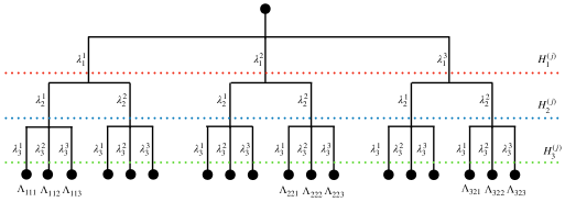
Figure 2: Construction of the frequency set $\tilde{\Omega}^{(j)}_{\mathcal{D}}$ from the data-encoding strategy $\mathcal{D}^{(j)}$.

Appendix B Proof of Theorem 1

We start by noting that Theorem 1 in the main text follows as an immediate corollary of the following Theorem:

Theorem 2: (RFF vs. variational QML – alternative form)

Let $R$ be the risk associated with a regression problem $P\sim\mathcal{X}\times\mathbb{R}$. Assume the following:

1. $\|f^{*}_{(\Theta,\mathcal{D},O)}\|_{K_{\mathcal{D}}}\leq C$,

2. $|y|\leq b$ almost surely when $(x,y)\sim P$, for some $b>0$.

Additionally, define

$$n_{0} \coloneqq\max\left\{4\|T_{K_{\mathcal{D}}}\|^{2},\left(528\log\frac{1112\sqrt{2}}{\delta}\right)^{2}\right\},$$ (109)

$$c_{0} \coloneqq 36\left(3+\frac{2}{\|T_{K_{\mathcal{D}}}\|}\right),$$ (110)

$$c_{1} \coloneqq 8\sqrt{2}(4b+\frac{5}{\sqrt{2}}C+2\sqrt{2C}).$$ (111)

Then, let $\delta\in(0,1]$, let $n\geq n_{0}$, set $\lambda_{n}=1/\sqrt{n}$, and let $\hat{f}_{M_{n},\lambda_{n}}$ be the output of $\lambda_{n}$-regularized linear regression with respect to the feature map

$$\phi_{M_{n}}(x)=\frac{1}{\sqrt{M_{n}}}\big{(}\psi(x,\nu_{1}),\ldots,\psi(x,\nu_{M})\big{)}$$ (112)

constructed from the integral representation of $K_{\mathcal{D}}$ by sampling $M_{n}$ elements from $\pi$. Then,

$$M_{n}\geq c_{0}\sqrt{n}\log\frac{108\sqrt{n}}{\delta}$$ (113)

is enough to guarantee, with probability at least $1-\delta$, that if $R(\hat{f}_{M_{n},\lambda_{n}})\geq R(f^{*}_{(\Theta,\mathcal{D},O)})$, then

$$R(\hat{f}_{M_{n},\lambda_{n}})-R(f^{*}_{(\Theta,\mathcal{D},O)})\leq\frac{c_{1}\log^{2}\frac{1}{\delta}}{\sqrt{n}}.$$ (114)

Next we note that Theorem 2 above – from which we derive Theorem 1 in the main text as an immediate corollary – is essentially a straightforward application of the generalization bound given as Theorem 1 in Ref. [RR17]. As such, we start our proof of Theorem 2 with a presentation of this result. To this end, we require first a few definitions. Firstly, given a kernel $K$, with associated RKHS $(\mathcal{H}_{K},\langle\cdot,\cdot\rangle_{K})$, we define $\mathcal{H}^{C}_{K}=\{f\in\mathcal{H}_{K}\,|\,\|f\|_{K}\leq C\}$ as the subset of functions in $\mathcal{H}_{K}$ with RKHS norm bounded by $C$. We define $\mathcal{F}^{C}_{\mathcal{D}}$ and $\mathcal{F}^{C}_{(\Theta,\mathcal{D},O)}$ analogously. Additionally, given a regression problem $P$ with associated risk $R$, we then define

$$f^{*}_{\mathcal{H}^{C}_{K}}=\operatorname*{arg\,min}_{f\in\mathcal{H}^{C}_{K}}\left[R(f)\right],$$ (115)

as the optimal function for $P$ in $\mathcal{H}^{C}_{K}$. Finally, recall that we denote by $T_{K}$ the kernel integral operator associated with the kernel $K$ (see Definition 3). With this in hand, we can state a slightly reformulated version of the RFF generalization bound proven in Ref. [RR17] (which in turn build on the earlier results of Ref. [SS15]).

Theorem 3: (Theorem 1 from [RR17])

Assume a regression problem $P\sim\mathcal{X}\times\mathbb{R}$. Let $K:\mathcal{X}\times\mathcal{X}\rightarrow\mathbb{R}$ be a kernel, and let $\mathcal{H}^{C}_{K}$ be the subset of the RKHS $\mathcal{H}_{K}$ consisting of functions with RKHS-norm upper bounded by some constant $C$. Assume the following:

1. K has an integral representation

   $$K(x,x^{\prime})=\int_{\Phi}\psi(x,\nu)\psi(x^{\prime},\nu)\,\mathrm{d}\pi(\nu).$$ (116)

2. The function $\psi$ is continuous in both variables and satisfies $|\psi(x,\nu)|\leq\kappa$ almost surely, for some $\kappa\in[1,\infty)$.

3. $|y|\leq b$ almost surely when $(x,y)\sim P$, for some $b>0$.

Additionally, define

$$\overline{B} \coloneqq 2b+2\kappa\max\{1,\|f^{*}_{\mathcal{H}^{C}_{K}}\|_{K}\},$$ (117)

$$\overline{\sigma} \coloneqq 2b+2\kappa\sqrt{\max\{1,\|f^{*}_{\mathcal{H}^{C}_{K}}\|_{K}\}},$$ (118)

and

$$n_{0} \coloneqq\max\left\{4\|T_{K}\|^{2},\left(264\kappa^{2}\log\frac{556\kappa^{3}}{\delta}\right)^{2}\right\},$$ (119)

$$c_{0} \coloneqq 9\left(3+4\kappa^{2}+\frac{4\kappa^{2}}{\|T_{K}\|}+\frac{\kappa^{4}}{4}\right),$$ (120)

$$c_{1} \coloneqq 8\big{(}\overline{B}\kappa+\overline{\sigma}\kappa+\max\{1,\|f^{*}_{\mathcal{H}^{C}_{K}}\|_{K}\}\big{)}.$$ (121)

Then, let $\delta\in(0,1]$, $n\geq n_{0}$, assume $\lambda_{n}=1/\sqrt{n}$, and let $\hat{f}_{M_{n},\lambda_{n}}$ be the output of $\lambda_{n}$-regularized linear regression with respect to the feature map

$$\phi_{M_{n}}(x)=\frac{1}{\sqrt{M_{n}}}\big{(}\psi(x,\nu_{1}),\ldots\psi(x,\nu_{M})\big{]}$$ (122)

constructed from the integral representation of $K$ by sampling $M_{n}$ elements from $\pi$. Then,

$$M_{n}\geq c_{0}\sqrt{n}\log\frac{108\kappa^{2}\sqrt{n}}{\delta}$$ (123)

is enough to guarantee, with probability at least $1-\delta$, that

$$R(\hat{f}_{M_{n},\lambda_{n}})-R(f^{*}_{\mathcal{H}^{C}_{K}})\leq\frac{c_{1}\log^{2}\frac{1}{\delta}}{\sqrt{n}}.$$ (124)

This statement demonstrates, that under reasonable assumptions, the estimator that is obtained with a number of random features proportional to $\mathcal{O}(\sqrt{n}\log n)$ achieves a $\mathcal{O}(1/\sqrt{n})$ learning error. We would now like to prove Theorem 2 by applying Theorem 3 to the classical PQC-kernel $K_{\mathcal{D}}$. To do this, we require the following Lemma:

Lemma 4: (Function set inclusions)

For any constant $C$ one has that

$$\mathcal{F}^{C}_{(\Theta,\mathcal{D},O)}\subseteq \,\mathcal{F}^{C}_{\mathcal{D}}\subseteq\mathcal{F}_{\mathcal{D}}\subseteq\mathcal{H}_{K_{\mathcal{D}}}$$

(125)

$$\mathcal{H}^{C}_{K_{\mathcal{D}}}.$$

Proof of Lemma 4.

The inclusions $\mathcal{F}^{C}_{(\Theta,\mathcal{D},O)}\subseteq\mathcal{F}^{C}_{\mathcal{D}}\subseteq\mathcal{F}_{\mathcal{D}}$ are immediate by definition. To prove $\mathcal{F}_{\mathcal{D}}\subseteq\mathcal{H}_{K_{\mathcal{D}}}$ we consider any $f_{v}\in\mathcal{F}_{\mathcal{D}}$ and let $\tilde{\mathcal{F}}$ be the image of $\mathcal{X}$ under $\phi_{\mathcal{D}}$. We can then write $v=v_{1}+v_{2}$ where $v_{1}\in\tilde{\mathcal{F}}$ and $v_{2}$ lies in the remainder. We then have that

$$f_{v}(x) =\langle v,\phi_{\mathcal{D}}(x)\rangle$$ (126)

$$=\langle v_{1},\phi_{\mathcal{D}}(x)\rangle+\langle v_{2},\phi_{\mathcal{D}}(x)\rangle$$ (127)

$$=\langle v_{1},\phi_{\mathcal{D}}(x)\rangle.$$ (128)

By definition – i.e. the fact that $v_{1}\in\tilde{\mathcal{F}}$ – we know that we can write

$$v_{1}=\sum_{j}\gamma_{j}\phi_{\mathcal{D}}(x_{j})$$ (129)

and therefore we see that

$$f_{v}(x) =\sum_{j}\gamma_{j}\langle\phi_{\mathcal{D}}(x_{j}),\phi_{\mathcal{D}}(x)\rangle_{\mathcal{F}}$$ (130)

$$=\sum_{j}\gamma_{j}K_{\mathcal{D}}(x_{j},x)$$ (131)

i.e. $f_{v}$ is indeed in the RKHS $\mathcal{H}_{K_{\mathcal{D}}}$. Finally, the inclusion $\mathcal{F}^{C}_{\mathcal{D}}\subseteq\mathcal{H}^{C}_{K_{\mathcal{D}}}$ now follows easily, as $\mathcal{F}^{C}_{\mathcal{D}}\subseteq\mathcal{F}_{\mathcal{D}}\subseteq\mathcal{H}_{K_{\mathcal{D}}}$ yields

$$f\in\mathcal{F}^{C}_{\mathcal{D}}\implies f\in\mathcal{H}_{K_{\mathcal{D}}},$$ (132)

and by definition

$$f\in\mathcal{F}^{C}_{\mathcal{D}}\implies\|f\|_{K_{\mathcal{D}}}\leq C$$ (133)

which together means that

$$f\in\mathcal{F}^{C}_{\mathcal{D}}\implies f\in\mathcal{H}^{C}_{K_{\mathcal{D}}}.$$ (134)

∎

With this in hand, we can now prove Theorem 2.

Proof of Theorem 2.

We start by recalling that, as shown in Section 4.4, for any reweighting vector $w$ the reweighted PQC-kernel $K_{(\mathcal{D},w)}$ has the integral representation

$$K_{(\mathcal{D},w)}(x,x^{\prime})=\frac{1}{2\pi}\int_{\mathcal{X}}\int_{0}^{2\pi}\sqrt{2}\cos(\langle\omega,x\rangle+\gamma)\sqrt{2}\cos(\langle\omega,x^{\prime}\rangle+\gamma)q_{(\mathcal{D},w)}(\omega)\,\,\mathrm{d}\gamma\mathrm{d}\nu,$$ (135)

where

$$q_{(\mathcal{D},w)}(\omega)=\sum_{i=0}^{|\Omega^{+}_{\mathcal{D}}|}\frac{w_{i}^{2}}{\|w\|^{2}_{2}}\delta(\omega-\omega_{i}).$$ (136)

As a result, for any reweighting, including $w=(1,\ldots,1)$, the kernel $K_{(\mathcal{D},w)}$ satisfies assumption (1) of Theorem 3 with

$$\psi(x,\nu)=\sqrt{2}\cos(\langle\omega,x\rangle+\gamma).$$ (137)

Given this, we note that $\psi$ is continuous in both variables and that $|\psi(x,\nu)|\leq\sqrt{2}$ for all $x,\nu$ – i.e., for any kernel $K_{(\mathcal{D},w)}$, assumption (2) of Theorem 3 is satisified with $\kappa=\sqrt{2}$.

Next, set the $C$ appearing in Theorem 3 to the constant $C$ appearing in assumption (1) of Theorem 2. More specifically, we apply Theorem 3 to the subset $\mathcal{H}_{K_{\mathcal{D}}}^{C}$, where $C$ is an upper bound on the RKHS norm of the optimal function for $P$ in $\mathcal{F}_{(\Theta,\mathcal{D},O)}$ – i.e. $\|f^{*}_{(\Theta,\mathcal{D},O)}\|_{K_{\mathcal{D}}}\leq C$. Doing this we obtain, via Theorem 3 and the fact that $\kappa=\sqrt{2}$, that provided all the conditions of Theorem 2 are satisfied, then

$$R(\hat{f}_{M_{n},\lambda_{n}})-R(f^{*}_{\mathcal{H}^{C}_{K_{\mathcal{D}}}})\leq\frac{c_{1}\log^{2}\frac{1}{\delta}}{\sqrt{n}}.$$ (138)

To achieve the statement of Theorem 1 we then use the assumption that $\|f^{*}_{(\Theta,\mathcal{D},O)}\|_{K_{\mathcal{D}}}\leq C$. More specifically, via Lemma 4 this assumption implies that $f^{*}_{(\Theta,\mathcal{D},O)}\in\mathcal{H}^{C}_{K_{\mathcal{D}}}$, which together with the definition of $f^{*}_{\mathcal{H}^{C}_{K_{\mathcal{D}}}}$ as the optimal function in $\mathcal{H}^{C}_{K_{\mathcal{D}}}$, allows us to conclude that

$$R(f^{*}_{(\Theta,\mathcal{D},O)})\geq R(f^{*}_{\mathcal{H}^{C}_{K_{\mathcal{D}}}}).$$ (139)

This then implies

$$R(\hat{f}_{M_{n},\lambda_{n}})-R(f^{*}_{(\Theta,\mathcal{D},O)}) \leq R(\hat{f}_{M_{n},\lambda_{n}})-R(f^{*}_{\mathcal{H}^{C}_{K_{\mathcal{D}}}})$$ (140)

$$\leq\frac{c_{1}\log^{2}\frac{1}{\delta}}{\sqrt{n}}\hskip 80.00012pt\text{[via Eq.~{}\eqref{eq:intermediate_step}]}$$ (141)

as per the statement of Theorem 2. ∎

As already mentioned, Theorem 1 in the main text then follows as an immediate corollary of Theorem 2.

Appendix C Proof of Lemma 1

Proof of Lemma 1.

As discussed in Ref. [RBD10], the kernel integral operator is self-adjoint. In light of this, we know that $\|T_{K_{(\mathcal{D},w)}}\|=\rho(T_{K_{(\mathcal{D},w)}})$, where $\rho(T_{K_{(\mathcal{D},w)}})$ denotes the spectral radius of $\rho(T_{K_{(\mathcal{D},w)}})$. As such, we focus on determining the spectrum of $\rho(T_{K_{(\mathcal{D},w)}})$. To this end, note that under assumption (a) of the lemma statement we have that

$$(T_{K_{(\mathcal{D},w)}}g)(x) =\int_{\mathcal{X}}K_{(\mathcal{D},w)}(x,x^{\prime})g(x^{\prime})dP_{\mathcal{X}}(x^{\prime})$$ (142)

$$=\frac{1}{(2\pi)^{d}}\int_{\mathcal{X}}K_{(\mathcal{D},w)}(x,x^{\prime})g(x^{\prime})\,\mathrm{d}x^{\prime}\qquad\qquad\text{[via assumption (a)]}$$ (143)

with

$$K_{(\mathcal{D},w)}(x,x^{\prime}) =\frac{1}{\|w\|^{2}_{2}}\left(w^{2}_{0}+\sum_{i=1}^{|\Omega^{+}_{\mathcal{D}}|}w_{i}^{2}\cos(\langle\omega_{i},(x-x^{\prime})\rangle)\right)$$ (144)

where $\omega_{0}=(0,\ldots,0)$. We now use assumption (b) – i.e. that $\Omega_{\mathcal{D}^{+}}\subset\mathbb{Z}^{d}$ – to show that for any $\omega\in\mathbb{Z}^{d}$, the function $g(x^{\prime})=\cos(\langle\omega,x^{\prime}\rangle)$ is an eigenfunction of $T_{K_{(\mathcal{D},w)}}$. Specifically, using the following notation

$$\delta(\omega\pm\nu)\coloneqq\begin{cases}1\hskip 10.00002pt\text{if }(\omega=\nu)\lor(\omega=-\nu),\\ 0\hskip 10.00002pt\text{else},\end{cases}$$ (146)

and defining $w_{\omega}$ to be the weight associated with $\omega\in\Omega_{\mathcal{D}}$, we have that

$$(T_{K_{(\mathcal{D},w)}}g)(x) =\frac{1}{(2\pi)^{d}}\int_{\mathcal{X}}\left[\frac{1}{\|w\|^{2}_{2}}\left(w^{2}_{0}+\sum_{i=1}^{|\Omega^{+}_{\mathcal{D}}|}w_{i}^{2}\cos(\langle\omega_{i},(x-x^{\prime})\rangle)\right)\right]\cos(\langle\omega,x^{\prime}\rangle)\,\mathrm{d}x^{\prime}$$ (147)

$$=\frac{1}{(2\pi)^{d}\|w\|_{2}^{2}}\left[\int_{\mathcal{X}}w^{2}_{0}\cos(\langle\omega,x^{\prime}\rangle)\,\mathrm{d}x^{\prime}+\int_{\mathcal{X}}\sum_{i=1}^{|\Omega^{+}_{\mathcal{D}}|}w_{i}^{2}\cos(\langle\omega_{i},(x-x^{\prime})\rangle)\cos(\langle\omega,x^{\prime}\rangle)\,\mathrm{d}x^{\prime}\right]$$ (148)

$$=\frac{1}{(2\pi)^{d}\|w\|_{2}^{2}}\int_{\mathcal{X}}\sum_{i=1}^{|\Omega^{+}_{\mathcal{D}}|}w_{i}^{2}\cos(\langle\omega_{i},(x-x^{\prime})\rangle)\cos(\langle\omega,x^{\prime}\rangle)\,\mathrm{d}x^{\prime}\hskip 30.00005pt\text{[via assumption (b)]}$$ (149)

$$=\frac{1}{(2\pi)^{d}\|w\|_{2}^{2}}\sum_{i=1}^{|\Omega^{+}_{\mathcal{D}}|}w_{i}^{2}\int_{\mathcal{X}}\cos(\langle\omega_{i},(x-x^{\prime})\rangle)\cos(\langle\omega,x^{\prime}\rangle)\,\mathrm{d}x^{\prime}$$ (150)

$$=\frac{1}{(2\pi)^{d}\|w\|^{2}_{2}}\sum_{i=1}^{|\Omega^{+}_{\mathcal{D}}|}w_{i}^{2}\frac{(2\pi)^{d}}{2}\cos(\langle\omega_{i},x\rangle)\delta(\omega_{i}\pm\omega)\hskip 75.0001pt\text{[via assumption (b)]}$$ (151)

$$=\begin{cases}\frac{w_{\omega}^{2}}{2\|w\|^{2}_{2}}\cos(\langle\omega,x\rangle)\hskip 10.00002pt\text{if }\omega\in\Omega^{+}_{\mathcal{D}},\\ \frac{w_{-\omega}^{2}}{2\|w\|^{2}_{2}}\cos(\langle\omega,x\rangle)\hskip 10.00002pt\text{if }\omega\in-\Omega^{+}_{\mathcal{D}},\\ 0\hskip 68.00012pt\text{else}.\end{cases}$$ (152)

A similar calculation shows that, for all $\omega\in\mathbb{Z}^{d}$,

$$\left(T_{K_{(\mathcal{D},w)}}\sin(\langle\omega,x^{\prime}\rangle)\right)(x)=\begin{cases}\frac{w_{\omega}^{2}}{2\|w\|^{2}_{2}}\sin(\langle\omega,x\rangle)\hskip 20.00003pt\text{if }\omega\in\Omega^{+}_{\mathcal{D}},\\ \frac{w_{-\omega}^{2}}{2\|w\|^{2}_{2}}\sin(\langle\omega,x\rangle)\hskip 10.00002pt\text{if }\omega\in-\Omega^{+}_{\mathcal{D}},\\ 0\hskip 72.00008pt\text{else}.\end{cases}$$ (153)

As such, we have that all functions in the set $\{\sin\langle\omega,x\rangle)\,|\,\omega\in\mathbb{Z}^{d}\}\cup\{\cos\langle\omega,x\rangle)\,|\,\omega\in\mathbb{Z}^{d}\}$ are eigenfunctions of $T_{K_{\mathcal{D}}}$. However, as this set is a basis for $L^{2}(\mathcal{X},P_{\mathcal{X}})$ – in the relevant case where $P_{\mathcal{X}}$ is the uniform distribution – we can conclude that

$$\|T_{K_{(\mathcal{D},w)}}\| =\rho\left(T_{K_{(\mathcal{D},w)}}\right)$$ (154)

$$=\max_{\omega\in\Omega_{\mathcal{D}}}\left\{\frac{1}{2}\frac{w_{\omega}^{2}}{\|w\|^{2}_{2}}\right\}$$ (155)

$$=\max_{\omega\in\Omega_{\mathcal{D}}}\left\{\frac{1}{2}p_{(\mathcal{D},w)}(\omega)\right\}.$$ (156)

∎

As an aside, it is interesting to note that the minimization of the norm $\|T_{K_{(\mathcal{D},w)}}\|$ subject to the constraint $\|w\|^{2}_{2}\leq c_{0}$ for some $c_{0}>0$ can be captured in terms of a convex semi-definite problem. This problem can be written as

minimize $$c$$ (157)

$$\text{subject to }\frac{1}{2}\frac{w_{\omega}^{2}}{\|w\|^{2}_{2}} \leq c,$$ (158)

$$\|w\|^{2}_{2} \leq c_{0},$$ (159)

which is easily seen to be equivalent with

minimize $$c$$ (160)

$$\text{subject to }\left[\begin{array}[]{cc}2c&|w_{\omega}|\\ |w_{\omega}|&d\end{array}\right] \geq 0\,\text{for all }\omega,$$ (163)

$$d \leq c_{0},$$ (164)

$$\left[\begin{array}[]{cc}d&w\\ w^{T}&I\end{array}\right] \geq 0,$$ (167)

by making use of Schur complements.

Appendix D Proof of Lemma 3

Proof of Lemma 3.

As $g_{\vec{\omega}}(x)$ is the output of the RFF procedure in which frequencies $\vec{\omega}=(\omega_{1},\ldots,\omega_{M})$ were drawn, we know that $g_{\vec{\omega}}$ can be written as

$$g_{\vec{\omega}}(x)=\sum_{\omega\in\tilde{\Omega}_{\mathcal{D}}}\hat{g}_{\vec{\omega}}(\omega)e^{i\langle\omega,x\rangle},$$ (168)

where $\hat{g}_{\vec{\omega}}(\omega)=0$ for all $\omega\notin\{\omega_{i}\}|_{i=1}^{M}$. Again we abuse notation and use $\hat{g}_{\vec{\omega}}$ to denote the vector with entries $\hat{g}_{\vec{\omega}}(\omega)$. Now, given some vector $\vec{\omega}=(\omega_{1},\ldots,\omega_{M})\in\Omega^{M}_{\mathcal{D}}$, we define the sets $\Omega_{\vec{\omega}}\coloneqq\{\omega_{1},\ldots,\omega_{M}\}\subseteq\Omega_{\mathcal{D}}$ and $\tilde{\Omega}_{\vec{\omega}}\coloneqq\Omega_{\vec{\omega}}\cup(-\Omega_{\vec{\omega}})$. Given some $\hat{f}^{*}$, we then define the vectors

$$\hat{f}^{*}_{\vec{\omega}}(\omega) =\begin{cases}\hat{f}^{*}(\omega)\text{ if }\omega\in\tilde{\Omega}_{\vec{\omega}},\\ 0\text{ else},\end{cases}$$ (169)

$$\hat{f}^{*}_{/\vec{\omega}}(\omega) =\begin{cases}0\text{ if }\omega\in\tilde{\Omega}_{\vec{\omega}},\\ \hat{f}^{*}(\omega)\text{ else}.\end{cases}$$ (170)

Note that with these definitions, $\hat{f}^{*}=\hat{f}^{*}_{\vec{\omega}}+\hat{f}^{*}_{/\vec{\omega}}$. Using this, we have that

$$\|\hat{f}^{*}-\hat{g}_{\vec{\omega}}\|_{2}^{2} =\|\hat{f}^{*}_{\vec{\omega}}+\hat{f}^{*}_{/\vec{\omega}}-\hat{g}_{\vec{\omega}}\|_{2}^{2}$$ (171)

$$=\|\hat{f}^{*}_{/\vec{\omega}}\|^{2}_{2}+\|\hat{f}^{*}_{\vec{\omega}}-\hat{g}_{\vec{\omega}}\|_{2}^{2}$$ (172)

$$\geq\|\hat{f}^{*}_{/\vec{\omega}}\|^{2}_{2}$$ (173)

$$=\|\hat{f}^{*}\|^{2}_{2}-\|\hat{f}^{*}_{\vec{\omega}}\|_{2}^{2}.$$ (174)

Using this expression, we can then lower-bound $\hat{\epsilon}$, the expected $L^{2}$-norm of the difference between the optimal PQC function and the output of the RFF procedure, recalling that $\xi(\vec{\omega})$ is the probability of sampling the vector of frequencies $\vec{\omega}$:

$$\hat{\epsilon} =\sum_{\vec{\omega}\in\Omega^{M}_{\mathcal{D}}}\|f^{*}-g_{\vec{\omega}}\|_{2}^{2}\,\xi(\vec{\omega})$$ (175)

$$=(2\pi)^{d}\sum_{\vec{\omega}\in\Omega^{M}_{\mathcal{D}}}\|\hat{f}^{*}-\hat{g}_{\vec{\omega}}\|_{2}^{2}\xi(\vec{\omega})\hskip 50.00008pt\text{ [via Parseval's identity]}$$ (176)

$$\geq(2\pi)^{d}\sum_{\vec{\omega}\in\Omega^{M}_{\mathcal{D}}}\left[\|\hat{f}^{*}\|^{2}_{2}-\|\hat{f}^{*}_{\vec{\omega}}\|_{2}^{2}\right]\xi(\vec{\omega})\hskip 30.00005pt\text{ [via Eq.~{}\eqref{eq:two_norm_split}]}$$ (177)

$$=(2\pi)^{d}\|\hat{f}^{*}\|^{2}_{2}-(2\pi)^{d}\sum_{\vec{\omega}\in\Omega^{M}_{\mathcal{D}}}\|\hat{f}^{*}_{\vec{\omega}}\|_{2}^{2}\,\xi(\vec{\omega}).$$ (178)

Using the short-hand notation $0$ to denote the frequency vector $(0,\ldots,0)$, we can now analyze the final term as

$$\sum_{\vec{\omega}\in\Omega^{M}_{\mathcal{D}}}\|\hat{f}^{*}_{\vec{\omega}}\|_{2}^{2}\;\xi(\vec{\omega}) =\sum_{\begin{subarray}{c}\vec{\omega}\in\Omega^{M}_{\mathcal{D}}\\ 0\notin\Omega_{\vec{\omega}}\end{subarray}}\sum_{i=1}^{M}\left(|\hat{f}^{*}(-\omega_{i})|^{2}+|\hat{f}^{*}(\omega_{i})|^{2}\right)\xi(\vec{\omega})$$ (179)

$$\qquad\qquad+\sum_{\begin{subarray}{c}\vec{\omega}\in\Omega^{M}_{\mathcal{D}}\\ 0\in\Omega_{\vec{\omega}}\end{subarray}}\left[\sum_{i=1}^{M-1}\left(|\hat{f}^{*}(-\omega_{i})|^{2}+|\hat{f}^{*}(\omega_{i})|^{2}\right)+|\hat{f}^{*}(0)|^{2}\right]\xi(\vec{\omega})$$ (180)

$$\leq\sum_{\begin{subarray}{c}\vec{\omega}\in\Omega^{M}_{\mathcal{D}}\\ 0\notin\Omega_{\vec{\omega}}\end{subarray}}\sum_{i=1}^{M}2|\hat{f}^{*}(\omega_{i})|^{2}\xi(\vec{\omega})$$ (181)

$$\qquad\qquad+\sum_{\begin{subarray}{c}\vec{\omega}\in\Omega^{M}_{\mathcal{D}}\\ 0\in\Omega_{\vec{\omega}}\end{subarray}}\left[\sum_{i=1}^{M-1}2|\hat{f}^{*}(\omega_{i})|^{2}+2|\hat{f}^{*}(0)|^{2}\right]\xi(\vec{\omega})$$ (182)

$$=2\sum_{i=1}^{M}\sum_{\omega_{1}\in\Omega_{\mathcal{D}}}\cdot\cdot\cdot\sum_{\omega_{M}\in\Omega_{\mathcal{D}}}|\hat{f}^{*}(\omega_{i})|^{2}p(\omega_{1})\cdot\cdot\cdot p(\omega_{M})$$ (183)

$$=2\sum_{i=1}^{M}\sum_{\omega_{i}\in\Omega_{\mathcal{D}}}|\hat{f}^{*}(\omega_{i})|^{2}p(\omega_{i})$$ (184)

$$=2M\sum_{\nu\in\Omega_{\mathcal{D}}}|\hat{f}^{*}(\nu)|^{2}p(\nu).$$ (185)

Substituting Eq. (185) into Eq. (178) then gives the statement of the Lemma. ∎

References

- [ABK+] Eric R. Anschuetz, Andreas Bauer, Bobak T. Kiani and Seth Lloyd “Efficient classical algorithms for simulating symmetric quantum systems” DOI: 10.48550/arXiv.2211.16998
- [BLS+19] Marcello Benedetti, Erika Lloyd, Stefan Sack and Mattia Fiorentini “Parameterized quantum circuits as machine learning models” In Quantum Science and Technology 4.4 IOP Publishing, 2019, pp. 043001 DOI: 10.1088/2058-9565/ab4eb5
- [CAB+21] Marco Cerezo et al. “Variational quantum algorithms” In Nature Reviews Physics 3.9 Springer ScienceBusiness Media LLC, 2021, pp. 625–644 DOI: 10.1038/s42254-021-00348-9
- [CGM+21] Matthias C. Caro et al. “Encoding-dependent generalization bounds for parametrized quantum circuits” In Quantum 5 Verein zur Forderung des Open Access Publizierens in den Quantenwissenschaften, 2021, pp. 582 DOI: 10.22331/q-2021-11-17-582
- [FRD+22] Enrico Fontana, Ivan Rungger, Ross Duncan and Cristina Cîrstoiu “Spectral analysis for noise diagnostics and filter-based digital error mitigation”, 2022 arXiv:2206.08811 [quant-ph]
- [FRD+23] Enrico Fontana et al. “Classical simulations of noisy variational quantum circuits”, 2023 arXiv:2306.05400
- [FV12] Andrew J. Ferris and Guifre Vidal “Perfect sampling with unitary tensor networks” In Phys. Rev. B 85 American Physical Society, 2012, pp. 165146 DOI: 10.1103/PhysRevB.85.165146
- [GSP+19] Ivan Glasser et al. “Expressive power of tensor-network factorizations for probabilistic modeling, with applications from hidden Markov models to quantum machine learning” In Advances in Neural Information Processing Systems 32, Proceedings of the NeurIPS 2019 Conference, 2019 arXiv:1907.03741
- [GT20] Francisco Javier Gil Vidal and Dirk Oliver Theis “Input redundancy for parameterized quantum circuits” In Frontiers in Physics 8 Frontiers Media SA, 2020, pp. 297
- [JFN+23] Sofiene Jerbi et al. “Quantum machine learning beyond kernel methods” In Nature Communications 14, 2023, pp. 517 DOI: 10.1038/s41467-023-36159-y
- [JGM+23] Sofiene Jerbi et al. “Shadows of quantum machine learning”, 2023 arXiv:2306.00061
- [LSS+22] Martín Larocca et al. “Group-invariant quantum machine learning” In PRX Quantum 3.3 APS, 2022, pp. 030341
- [LTD+22] Jonas Landman et al. “Classically approximating variational quantum machine learning with random Fourier features” arXiv, 2022 arXiv:2210.13200
- [MMG+23] Johannes Jakob Meyer et al. “Exploiting Symmetry in Variational Quantum Machine Learning” In PRX Quantum 4 American Physical Society, 2023, pp. 010328 DOI: 10.1103/PRXQuantum.4.010328
- [MRT18] Mehryar Mohri, Afshin Rostamizadeh and Ameet Talwalkar “Foundations of machine learning” MIT press, 2018
- [pac] Tensor package “Sampling from an MPS”
- [RBD10] Lorenzo Rosasco, Mikhail Belkin and Ernesto De Vito “On learning with integral operators.” In Journal of Machine Learning Research 11.2, 2010
- [RR07] Ali Rahimi and Benjamin Recht “Random features for large-scale kernel machines” In Advances in neural information processing systems 20, 2007 DOI: 10.5555/2981562.2981710
- [RR17] Alessandro Rudi and Lorenzo Rosasco “Generalization properties of learning with random features” In Proceedings of the 31st International Conference on Neural Information Processing Systems, NIPS’17 Long Beach, California, USA: Curran Associates Inc., 2017, pp. 3218–3228
- [RSV16] Jen-Hao Rick Chang, Aswin C Sankaranarayanan and B… Vijaya Kumar “Random features for sparse signal classification” In Proceedings of the IEEE Conference on Computer Vision and Pattern Recognition, 2016, pp. 5404–5412
- [SC08] Ingo Steinwart and Andreas Christmann “Support vector machines” Springer Science & Business Media, 2008
- [Sch11] Ulrich Schollwöck “The density-matrix renormalization group in the age of matrix product states” In Annals of Physics 326.1 Elsevier BV, 2011, pp. 96–192 DOI: 10.1016/j.aop.2010.09.012
- [Sch21] Maria Schuld “Supervised quantum machine learning models are kernel methods” arXiv, 2021 arXiv:2101.11020
- [SEM23] Franz J. Schreiber, Jens Eisert and Johannes Jakob Meyer “Classical surrogates for quantum learning models” In Physical Review Letters 131, 2023, pp. 100803 DOI: 10.1103/PhysRevLett.131.100803
- [SS15] B.. Sriperumbudur and Z. Szabo “Optimal rates for random Fourier features”, 2015 arXiv:1506.02155
- [SS15a] Danica J. Sutherland and Jeff Schneider “On the error of random Fourier features” arXiv, 2015 arXiv:1506.02785
- [SSM21] Maria Schuld, Ryan Sweke and Johannes Jakob Meyer “Effect of data encoding on the expressive power of variational quantum-machine-learning models” In Phys. Rev. A 103 American Physical Society, 2021, pp. 032430 DOI: 10.1103/PhysRevA.103.032430
- [STJ23] Seongwook Shin, Yong Siah Teo and Hyunseok Jeong “Analyzing quantum machine learning using tensor network”, 2023 arXiv:2307.06937
- [SW10] Miles Stoudenmire and Steven R. White “Minimally entangled typical thermal state algorithms” In New Journal of Physics 12.5 IOP Publishing, 2010, pp. 055026 DOI: 10.1088/1367-2630/12/5/055026
- [SWC+23] Yuguo Shao, Fuchuan Wei, Song Cheng and Zhengwei Liu “Simulating quantum mean values in noisy variational quantum algorithms: A polynomial-scale approach”, 2023 arXiv:2306.05804