TOPPQuad: Dynamically-Feasible Time Optimal Path Parametrization for Quadrotors

Abstract

Planning time-optimal trajectories for quadrotors in cluttered environments is a challenging, non-convex problem. This paper addresses minimizing the traversal time of a given collision-free geometric path without violating bounds on individual motor thrusts of the vehicle. Previous approaches have either relied on convex relaxations that do not guarantee dynamic feasibility, or have generated overly conservative time parametrizations. We propose TOPPQuad, a time-optimal path parameterization algorithm for quadrotors which explicitly incorporates quadrotor rigid body dynamics and constraints such as bounds on inputs (including motor speeds) and state of the vehicle (including the pose, linear and angular velocity and acceleration). We demonstrate the ability of the planner to generate faster trajectories that respect hardware constraints of the robot compared to several planners with relaxed notions of dynamic feasibility. We also demonstrate how TOPPQuad can be used to plan trajectories for quadrotors that utilize bidirectional motors. Overall, the proposed approach paves a way towards maximizing the efficacy of autonomous micro aerial vehicles while ensuring their safety.

I Introduction

Autonomous micro aerial vehicles (MAVs) have demonstrated an immense potential to transform logistics in numerous domains. Package delivery in large metropolitan areas with dense traffic, aid distribution in disaster-stricken environments, and inventory management in large warehouses are only a few such examples. The unique combination of size and aerial agility makes MAVs ideal for navigating cluttered 3-D environments beyond the reach of other robots. However, key to realizing their full potential in boosting task productivity while ensuring safe environmental interaction lies in planning missions that respect their physical limitations. This work addresses a class of problems in planning dynamically-feasible time-optimal trajectories for MAVs.

Planning time-optimal trajectories for robots subject to actuation constraints in cluttered environments is a challenging task. First, the presence of obstacles renders the underlying optimization problem non-convex, even for systems with linear dynamics. Second, the high-dimensional non-Euclidean state space of most aerial vehicles makes trajectory synthesis subject to actuation constraints formidable, especially in obstacle-rich environments. One way of addressing these hurdles involves a decoupled approach to motion planning [1]. First, a sufficiently smooth collision-free geometric path is determined. It is then endowed with an optimal time parametrization that respects the actuation constraints of the robot. Our work focuses on the second stage, the minimization of the traversal time of a given geometric path while respecting individual motor thrusts bounds of the MAV.

A landmark result [2] previously established the differential flatness [3] of quadrotor dynamics. This initiated a line of computationally-efficient approaches [2, 4, 5] that optimize trajectories in the space of (piecewise) polynomials of quadrotor positions and yaw angles. It also demonstrated the highly non-convex dependence of motor thrusts on the underlying flat outputs. Most previous works either (a) use (convex) relaxations of actuation constraints [6], (b) use bounds on the total thrust and angular velocity instead of actual motor thrusts [7], or (c) plan dynamically feasible trajectories without clear bounds on suboptimality [5]. Our approach can be viewed as a generalization of [5] in that we use a spatially-varying dilation of time to transform any sufficiently smooth trajectory into a feasible one.

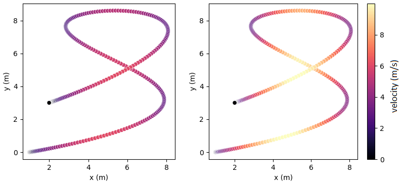
Figure 1: The square-speed profile over the course of a trajectory for a dynamically feasible $\alpha$-scaled minimum snap trajectory (left) and a TOPPQuad trajectory (right), plotted with respect to the trajectory velocity (m/s). The TOPPQuad trajectory decreased traversal by $2.97s$ ($37.3\%$) in a $28.9m$ trajectory.

Optimizing spatially-varying time dilations of a trajectory is also known as the time optimal path parametrization (TOPP) problem. Early works addressed this in the context of planning trajectories for manipulators subject to bounds on its joint velocities and torques [8]. Verscheure et al introduced the square speed profile, uncovering the hidden convexity behind such problems [9]. This approach has been adopted to many other robotic systems [10, 11], and various computational improvements to the original method have been proposed [12]. However, none of these approaches deal with the subtle bounds involved in planning rotational components of trajectories of the vehicle, which are critical. This is due to the inclusion of rotations which introduces non-convex constraints, even with the aid of the square speed profile. Addressing the rotational aspects of trajectory generation for MAVs is the core theme of this paper.

Various existing work has explored time-optimal quadrotor trajectory planning with individual motor speed constraints. Ryou et al uses Gaussian Processes to learn a time-optimal obstacle-free trajectory from repeated simulation results, but any changes to the set of waypoints or obstacle space requires re-training the network [13]. Foehn et al formulates the planning problem by trajectory ‘progress’ to find time-optimal trajectories and allows minor waypoint deviation, but in doing so assumes an sparse environment [14].

Towards this end, we propose TOPPQuad, a TOPP algorithm that considers the full rigid body dynamics of the quadrotor. The contributions of this paper are as follows:

• A trajectory planner capable of refining time-optimal trajectories obtained from any arbitrary planner.

• A method of planning time-optimal trajectories for a bidirectional quadrotor (i.e. one whose motor thrusts can be both parallel and antiparallel to its body $z$ axis), that seamlessly bypasses switching between flatness diffeomorphisms.

• A comparison of the resulting trajectories with existing planners in simulation and with real-world experimental data. We show that inclusion of rotational variables leads to faster dynamically feasible trajectories.

II Problem Formulation

We consider the problem of minimizing the traversal time of an arbitrary sufficiently smooth geometric path for an actuation-constrained quadrotor. A geometric path

$$\gamma:[0,S_{end}]\rightarrow\mathbb{R}^{3}.$$ (1)

is one not necessarily parametrized by time, but rather by some other abstract parameter denoted by $s\in[0,S_{end}]$, such as arc length. We model the quadrotor using the standard rigid body dynamics model given by

$$\underbrace{\begin{bmatrix}\dot{\mathbf{p}}\\ \dot{\mathbf{v}}\\ \dot{\mathbf{R}}\\ \dot{\mathbf{\omega}}\\ \end{bmatrix}}_{\dot{\mathbf{x}}}=\underbrace{\begin{bmatrix}\mathbf{v}\\ \mathbf{R}\mathbf{e}_{3}\ \frac{c}{m}+\mathbf{g}\\ \mathbf{R}[\omega\times]\\ \mathbf{J}^{-1}(\tau-\omega\times\mathbf{J}\omega)\\ \end{bmatrix}}_{\mathbf{f}(\mathbf{x},\mathbf{u})},$$ (2)

where the total thrust $c\in\mathbb{R}$ and torque $\tau\in\mathbb{R}^{3}$ are given by

$$\begin{bmatrix}c\\ \tau\\ \end{bmatrix}=\underbrace{\mathbf{F}}_{\in\mathbb{\mathbf{R}}^{4\times 4}}\begin{bmatrix}u_{1}\\ u_{2}\\ u_{3}\\ u_{4}\end{bmatrix}.$$ (3)

In Eq. (3), $\mathbf{F}$ is a constant scaled control matrix, and $\mathbf{u}=[u_{1},u_{2},u_{3},u_{4}]^{T}\in\mathbb{R}^{4}$ represents control inputs — the squared speeds of the four motors. The position of the vehicle’s center of mass with respect to (w.r.t.) the world frame is denoted by $\mathbf{p}\in\mathbb{R}^{3}$, its velocity by $\mathbf{v}$, the columns of $\mathbf{R}\in SO(3)$ encode its body axes as linear combinations of world axes ($\mathbf{e}_{1},\mathbf{e}_{2},\mathbf{e}_{3}$), and $\omega\in\mathbb{R}^{3}$ is the angular velocity of the quadrotor expressed in the body frame of the vehicle.

The minimum-time path traversal problem can then be specified as an optimization problem over execution time $T$ and a sufficiently smooth time parametrization function $\chi(\cdot)$:

$$\min_{\begin{subarray}{c}T>0,\\ \chi:[0,T]\rightarrow[0,S_{end}]\end{subarray}}T$$ (4)

$$\hskip 17.07164pts.t.\hskip 2.84526pt\chi(0)=0,\ \chi(T)=S_{end},$$

$$\hskip 34.1433pt\chi(\cdot)\ \text{increasing on }[0,S_{end}],$$

$$\hskip 34.1433pt\mathbf{p}(t)=\gamma(\chi(t)),\quad\text{(path following constraint)}$$

$$\hskip 34.1433pt\dot{\mathbf{x}}(t)=\mathbf{f}(\mathbf{x}(t),\mathbf{u}(t)),\quad\text{(dynamics constraint)}$$

$$\hskip 34.1433pt\mathcal{H}(\mathbf{x}(t),\chi(t))\leq 0,\hskip 34.1433pt\text{(state constraints)}$$

$$\hskip 34.1433ptu_{min}\leq\mathbf{u}(t)\leq u_{max}\hskip 11.38109pt\text{(actuation constraint)}.$$

The relation $\mathcal{H}(\mathbf{x}(t),\chi(t))\leq 0$ collects state constraints such as bounds on the velocity, acceleration, and angular velocity of the vehicle. Additional requirements could include pose constraints at specified points along $\gamma$ that ensure the robot can pass through narrow gaps.

III Methodology

III-A Problem Reparametrization

Solving Problem (4) for many types of robots is easier upon introduction of the square speed profile [9, 10], defined via $h(s):=\left(\frac{ds}{dt}(s)\right)^{2}$ for all $s\in[0,S_{end}]$. When $s$ represents the arc length of $\gamma$, $h$ represents the square speed of the robot as a function of the distance it has traversed along the path. One motivation for the square speed profile comes from the elementary relation $\Delta v^{2}=2a\Delta s$; a bound on the maximum acceleration is equivalent to a bound on the Lipschitz constant of $v^{2}$ (i.e. $h$) w.r.t. $s$ — a linear (and thus convex) constraint [9, 15, 16]. In addition, we rewrite the orientation kinematics ($\dot{\mathbf{R}}=\mathbf{R}[\omega\times]$) as

$$\dot{\mathbf{q}}(t)=\frac{1}{2}\Omega(\omega)\mathbf{q}(t),$$ (5)

where $\mathbf{q}(t)\in S^{3}$ is a quaternion representing the rotation matrix $\mathbf{R}$, and

$$\Omega(\omega):=\begin{bmatrix}0&-\omega^{T}\\ \omega&-[\omega\times]\\ \end{bmatrix}.$$ (6)

Let $\gamma^{\prime}=d\gamma/ds$ and $\dot{\gamma}=d\gamma/dt$. Using the relation $\frac{d}{dt}=\frac{ds}{dt}\frac{d}{ds}=\sqrt{h(s)}\frac{d}{ds}$, we rewrite the objective and dynamics as follows. The objective function can be recovered as

$$T=\int_{0}^{S_{end}}dt=\int_{0}^{S_{end}}\frac{dt}{ds}ds=\int_{0}^{S_{end}}\frac{1}{\sqrt{h(s)}}ds.$$ (7)

We next unpack and rewrite the dynamic constraints in Problem (4). For the translational dynamics, the crucial relation is $\mathbf{p}(s)=\gamma(s)$. Differentiating, we get

$$\dot{\mathbf{p}}=\sqrt{h(s)}\mathbf{p}^{\prime}(s)=\sqrt{h(s)}\gamma^{\prime}(s),$$ (8)

$$\dot{\mathbf{v}}=\frac{1}{2}\gamma^{\prime}(s)h^{\prime}(s)+\gamma^{\prime\prime}(s)h(s).$$ (9)

Substituting these into the second line of Eq. (2),

$$\frac{1}{2}\gamma^{\prime}(s)h^{\prime}(s)+\gamma^{\prime\prime}(s)h(s)=\mathbf{R}(s)\mathbf{e}_{3}\ \frac{c(s)}{m}+\mathbf{g}.$$ (10)

For the rotational dynamics, we write with a slight abuse of notation

$$\mathbf{q}^{\prime}(s)=\frac{1}{2}\Omega([\omega(s)\times])\mathbf{q}(s).$$ (11)

To clarify, we abused notation in the expression above in that the relationship between $\omega$ from Eq. (5) and (11) is

$$\omega(t)=\sqrt{h(s)}\omega(s).$$ (12)

Noting the parallel between Eq. (8) and (12), and defining

$$\alpha(s):=\omega^{\prime}(s),$$ (13)

we get the relation

$$\dot{\omega}=\frac{1}{2}\omega(s)h^{\prime}(s)+\alpha(s)h(s).$$ (14)

This ultimately allows us to rewrite line 4 of Eq. (2) as

$$\tau=\mathbf{J}\underbrace{\left(\frac{1}{2}\omega(s)h^{\prime}(s)+\alpha(s)h(s)\right)}_{=\ \dot{\omega}}+\omega(s)\times\mathbf{J}\omega(s)\ h(s).$$ (15)

Combining Eq. (10) and (15), we get that the individual motor thrusts at point $s$ along the path are related to the translational and angular accelerations via

$$\begin{bmatrix}m(\frac{1}{2}\gamma^{\prime}(s)h^{\prime}(s)+\gamma^{\prime\prime}(s)h(s)-\mathbf{g})\\ \mathbf{J}\left(\frac{1}{2}\omega(s)h^{\prime}(s)+\alpha(s)h(s)\right)+\omega(s)\times\mathbf{J}\omega(s)\ h(s)\\ \end{bmatrix}$$ (16)

$$=\begin{bmatrix}\mathbf{R}(s)\mathbf{e}_{3}&0\\ 0&\mathbf{I}_{3}\\ \end{bmatrix}\mathbf{F}\mathbf{u}$$

III-B Numerical Implementation

To solve Problem (4), we therefore use the following decision variables:

$$h(\cdot),\ h^{\prime}(\cdot),\ \mathbf{q}(\cdot),\ \omega(\cdot),\ \alpha(\cdot),\ \mathbf{u}(\cdot),$$ (17)

which are all functions on $[0,S_{end}]$ as related by equations in part III-A. We approximately represent these functional decision variables by their values at a finite set of grid points $D=(0=s_{0}<s_{1}<\cdots<s_{N}=S_{end})$ where each consecutive pair is spaced $\Delta s$ apart. Thus, $h_{i}:=h(s_{i})$ and similarly for the remaining variables in Eq. (17). Furthermore, the differential constraints are approximated using forward Euler integration. As such, the effective dynamic constraints for $h(\cdot)$ and $\omega(\cdot)$ become

$$\begin{bmatrix}h_{i+1}\\ \omega_{i+1}\\ \end{bmatrix}=\begin{bmatrix}h_{i}+h_{i}^{{}^{\prime}}\ \Delta s\\ \omega_{i}+\alpha_{i}\ \Delta s\end{bmatrix}$$ (18)

$$\begin{bmatrix}m(\frac{1}{2}\gamma_{i}^{{}^{\prime}}h_{i}^{{}^{\prime}}+\gamma_{i}^{{}^{\prime\prime}}h_{i}-\mathbf{g})\\ J\left(\frac{1}{2}\omega_{i}h_{i}^{{}^{\prime}}+\alpha_{i}h_{i}\right)+\omega_{i}\times J\omega_{i}\ h_{i}\\ \end{bmatrix}=\begin{bmatrix}\mathbf{R}_{i}\mathbf{e}_{3}&0\\ 0&\mathbf{I}_{3}\\ \end{bmatrix}\mathbf{F}\mathbf{u}_{i}.$$ (19)

Actuation constraints amount to $\mathbf{u}_{i}\in[u_{min},u_{max}]^{4}$, whereas the objective function, the total execution time, equals

$$T=\sum_{i=0}^{N-1}\frac{2\Delta s}{\sqrt{h_{i}}+\sqrt{h_{i+1}}}.$$ (20)

The critical numerical approximation we make is in the rotational kinematics. In particular, we approximate the dynamics of $q$ via

$$\mathbf{q}_{i+1}=\frac{(\mathbf{I}_{4}+\frac{\Delta s}{2}\Omega(\omega_{i}))\ \mathbf{q}_{i}}{\sqrt{1+\frac{\Delta s^{2}}{4}||\omega_{i}||_{2}^{2}}},$$ (21)

where $\mathbf{I}_{4}$ denotes the $4\times 4$ identity matrix. The numerator of Eq. (21) represents the first-order Euler integration of quaternion kinematics, whereas the denominator projects this value back onto $S^{3}$, the manifold of quaternions.

IV Experimental Setup

We benchmark TOPPQuad against a family of flatness-based planners and alternate TOPP procedures based on convex relaxations of dynamic constraints. All planners are written in Python and computed on a laptop with an i7-6700HQ CPU. The flatness-based planners are implemented with a linear least-squares program [17], the TOPP methods with cvxpy [18], and our TOPPQuad algorithm with the CasADi interface to IPOPT [19]. The planners are compared on a set of 200 randomized trajectories, each formed by interpolating four waypoints sampled from a $10m\times 10m\times 10m$ box. We use quadrotor parameters from the CrazyFlie 2.0 from bitcraze [20], including motor speed bounds of $[0,2500]$ $rad/s$.

IV-A Baselines

We select three sets of commonly-used baselines: minimum snap, minimum jerk, and minimum acceleration [5]. Within each set, we apply three types of constraints while ensuring the geometric path remains fixed:

IV-A1 The unconstrained flatness-based trajectory planner

Waypoint visit times are pre-assigned, with the time interval between consecutive waypoints determined from their Euclidean distance and a nominal velocity $v$.

IV-A2 An upper bound on the maximum speed along the path

This approach solves a convex relaxation of the TOPP problem on the path generated from 1) by placing an equivalent bound on the squared speed profile.

$$\min \sum_{i=0}^{N-1}\frac{2\Delta s}{\sqrt{h_{i}}+\sqrt{h_{i+1}}}+\lambda\sum_{i=0}^{N}(h_{i}^{(3)})^{2}\quad$$ (22)

$$s.t. 0\leq h_{i}\leq\frac{v_{max}^{2}}{||\gamma_{i}^{\prime}||_{2}^{2}}\quad\forall i\leq N.$$

IV-A3 An upper bound on the maximum speed and total thrust magnitude

The TOPP problem is modified to include bounds on the maximum thrust:

$$\min \sum_{i=0}^{N-1}\frac{2\Delta s}{\sqrt{h_{i}}+\sqrt{h_{i+1}}}+\lambda\sum_{i=0}^{N}(h_{i}^{(3)})^{2}\quad$$ (23)

$$s.t. 0\leq h_{i}\leq\frac{v_{max}^{2}}{||\gamma_{i}^{\prime}||_{2}^{2}}$$

$$\left|\left|\frac{1}{2}\gamma_{i}^{{}^{\prime}}h_{i}^{{}^{\prime}}+\gamma_{i}^{{}^{\prime\prime}}h_{i}-\mathbf{g}\right|\right|_{2}\leq 4u_{max}\quad\forall i\leq N.$$

We represent the square speed profile as a third-order integrator to ensure a $\mathcal{C}^{3}$ trajectory. We add a regularization term $\lambda\sum_{i=0}^{N}(h_{i}^{(3)})^{2}$ to the objectives of Eq. (22) and (LABEL:eq:topp_acc) for a small positive $\lambda$ to ensure our optimization problems are numerically well conditioned. The sub-optimality of the solutions of convex relaxations decreases as $\lambda\downarrow 0$, but non-vanishing values of $\lambda$ are necessary for the solver to converge. In our experiments, we chose $\lambda=10^{-1}$.

We refer to “$\alpha$-scaling” ($\alpha$) as the method introduced in [5], which slows down the time uniformly across the trajectory until all the actuation constraints (i.e. motor speeds) lie within allowed ranges. This is equivalent to multiplying the square speed profile and its spatial derivatives by a suitable quantity (less than one). We perform $\alpha$-scaling on each of the baselines mentioned above to enforce dynamic feasibility.

IV-B Initial Guess

TOPPQuad requires an initial guess of variables in Eq. (17), the quality of which can greatly affect optimizer performance. For these comparisons, the initial guess is supplied from the baseline trajectories. To determine a ‘good’ initial guess, we examine the effect of three parameters: the planner’s nominal velocity $v$, the constraints on the planner, and $\Delta s$ determined by the number of discretization points $N$. Failure is considered to be one of two cases: when the CasADi solver fails to find a solution, and when the solver settles on a local minimum with a significantly slower traversal time than the initial guess.

We see that of three nominal velocities, $v=1m/s$ offers the best performance in both iteration count and success rate, as shown in Table I. A further examination shows that of the three cases considered, only at $v=1m/s$ do the resulting motor speeds consistently stay within the input bounds of the quadrotor. We then compare in Table II the algorithm’s optimization success rate given initial guesses from four planners: 1) a minimum snap (MS) trajectory computed with $v=1m/s$, 2) an $\alpha$-scaled minimum snap trajectory computed with some higher $v$, 3) an $\alpha$-scaled TOPP trajectory with only speed bounds, and 4) an $\alpha$-scaled TOPP trajectory with speed and acceleration bounds. We see that the minimum snap initial guesses have the highest success rates. We postulate that an initial guess with motor speeds far from the bounds of the input constraints is more likely to succeed, and in fewer iterations. From these results, we proceed using only the flatness-based planner initial guess, with $v=1m/s$.

Nominal Velocity ($v$)	1m/s	3m/s	5m/s
Avg Iterations	473	659	1138
Success Rate	0.981	0.918	0.609

TABLE I: TOPPQuad Initial Guess Success - Velocity Comparison

For the trajectories in this experiment, we find $N=300$ ($\Delta s\approx 0.025$) adquately satisfies requirements for optimizer convergence. Selecting $N$ too coarsely will see IPOPT frequently failing to converge, as the discrete dynamics in Eq. (19), (21) no longer accurately model the continuous dynamics in Eq. (16). On the other hand, selecting $N$ too finely will drastically increase run time for diminishing returns.

	MS (1 m/s)	$\alpha$ MS	$\alpha$ TOPP vel	$\alpha$ TOPP acc
Success Rate	0.991	0.981	0.936	0.891

TABLE II: TOPPQUad Initial Guess Success - Planner Comparison

V Comparison of Planning Algorithms

In this section, we first demonstrate the effectiveness of our algorithm along two metrics: dynamic feasibility and time optimality. In dynamic feasibility, we compare our optimized trajectories against the aforementioned baselines. In time optimality, we compare our algorithm against only the dynamically feasible $\alpha$-scaled baselines. Next, we extend our formulation to trajectory generation for bidirectional quadrotors. Finally, we apply our algorithm to real-world trajectories based on odometry data.

For a fair comparison, we bound the velocity magnitude of our planner and the TOPP planners to $5m/s$, and use $v=5m/s$ as the nominal velocity for the flatness-based planners. The computed trajectories average $27.5m$ in length for the minimum snap planner, $26.8m$ for the minimum jerk planner, and $21.4m$ for the minimum acceleration planner.

V-A Dynamic Feasibility

We measure dynamic feasibility by the percentage of trajectories that stay within motor speed bounds. Fig. 2 shows that even though trajectories have constraints on velocity and acceleration, they often require inputs that strongly exceed allowed motor speed bounds. Next, we focus only on the motor speeds of dynamically feasible planners, including TOPPQuad (Fig. 3). While all planners generate trajectories that respect motor speed constraints, the three baseline methods are conservative compared to the TOPPQuad trajectories, and do not always take full advantage of the quadrotor’s flight capabilities.

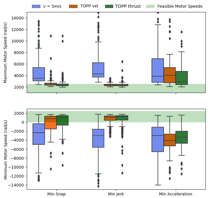
Figure 2: The distribution of maximum (top) and minimum (bottom) motor speeds over 200 randomized trajectories for three sets of planners: minimum snap (left), minimum jerk (middle), and minimum acceleration (right). In each set, we compare a flatness-based planner at $v=5m/s$ (blue), a TOPP planner subject to velocity constraints (orange), and a TOPP planner subject to velocity and thrust constraints (green). No planner consistently plans trajectories that stay within motor speed bounds.

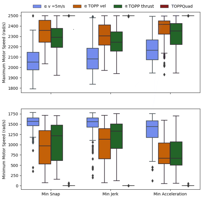
Figure 3: The distribution of maximum (top) and minimum (bottom) motor speeds over 200 randomized trajectories for three sets of $\alpha$-scaled planners: minimum snap (left), minimum jerk (middle), and minimum acceleration (right). In each set, we compare against an $\alpha$-scaled flatness-based planner (blue), an $\alpha$-scaled TOPP planner subject to velocity constraints (orange), and an $\alpha$-scaled TOPP planner subject to velocity and thrust constraints (green). Only TOPPQuad (red) is able to take full range of the quadrotor’s inputs.

V-B Time Optimality

Here, we focus on the time optimality of the dynamically feasible trajectory planners: the $\alpha$-scaled methods and TOPPQuad. Fig. 4 shows that our TOPPQuad method consistently generates faster trajectories than the $\alpha$-scaled methods. We see anywhere between a $2-5$ sec decrease from the unconstrained trajectories and about a $2$ sec decrease from the TOPP trajectories. This corresponds to an approximate $1.8m/s$ and $0.8m/s$ increase in respective average trajectory velocity. Note that the shorter average speed of the minimum acceleration trajectories is due to the faster average trajectory, not algorithm performance.

In Fig. 5, we show the percentage time decrease between our method and the three dynamically feasible baselines for the minimum snap case, as well as the $v=1m/s$ initial guess. For the $\alpha$-scaled minimum snap planner, the majority of trajectories see a time decrease of $40\%$ or more, and even the TOPP methods see at least a $10\%$ decrease.

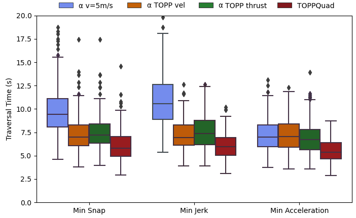
Figure 4: The distribution of traversal times over 200 randomized trajectories for three sets of $\alpha$-scaled planners: minimum snap (left), minimum jerk (middle), and minimum acceleration (right). In each set, we compare the traversal time for a $\alpha$-scaled flatness-based planner (blue), an $\alpha$-scaled TOPP planner subject to velocity constraints (orange), an $\alpha$-scaled TOPP planner subject to velocity and thrust constraints (green), and our TOPPQuad algorithm (red).

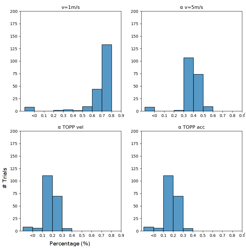
Figure 5: The distribution of traversal time improvement over the four dynamically feasible planners when refined with TOPPQuad: min snap $v=1m/s$ (top left), $\alpha$-scaled $v=5m/s$ min snap (top right), $\alpha$-scaled TOPP w/velocity constraints (bottom left), and $\alpha$-scaled TOPP w/acceleration constraints (bottom right). Values are computed against the initial $v=1m/s$ trajectory guess. Our algorithm consistently sees improvements in total traversal time, even against other time-optimal methods.

V-C Bidirectionality

The TOPP algorithm can be adapted for optimizing trajectories for bidirectional quadrotors, while sidestepping the difficulties of planning for a flatness-based model [21]. Such vehicles are governed by the same set of rigid body dynamics as ’unidirectional’ quadrotors, but can also exert thrust along the negative body $z$-axis of the robot. In particular, at each moment in time, the thrust of the four motors is given by the vector $u\in\mathbb{R}^{4}$ with coordinates $u_{j}=sign(u_{j})\omega_{j}^{2},\ 1\leq j\leq 4$. Here $\omega_{j}\in[0,\omega_{max}]$ represents the speed of motor $j$, and $sign(u_{j})\in\{+1,-1\}$ the direction of its thrust.

Towards optimizing trajectories with such input constraints, one possible approach involves introducing additional integral decision variables $(sign(u_{j,i}))_{1\leq j\leq 4,0\leq i\leq N}\in\{-1,+1\}^{4\times(N+1)}$ (with $j$ indexing the motors, and $i$ indexing the discretization points). However, solving mixed integer problems with a large number of integral variables ($N\sim 200$) is typically computationally expensive. To work around this challenge, we instead introduce continuous decision variables $z_{j,i}\in[-1,+1]$, and represent the thrust of motor $j$ at discretization point $i$ as $u_{j}=z_{j,i}\omega_{j,i}^{2}$, where $\omega_{j,i}\in[0,\omega_{max}]$. In light of the fact that

$$z_{j,i}\omega_{j,i}^{2}=\underbrace{sign(z_{j,i})}_{=:sign(u_{j,i})}(\underbrace{\sqrt{|z_{j,i}|}\ \omega_{j,i}}_{\in[0,\omega_{max}]})^{2},$$ (24)

our re-parametrization leaves the set of feasible inputs intact.

We ultimately use the adapted method to compare time optimal parametrizations for unidirectional and bidirectional quadrotors with the same mass, moment of inertia, and maximum motor speeds. The purpose of this example is to see how much efficiency can be gained by using bidirectional motors. With the $v=5m/s$ constraint, we see a traversal time performance on par with the unidirectional quad. This can likely be attributed to the saturation of the maximum velocity constraint, preventing any further time improvements.

In Fig. 6, we show the same trajectory computed for a time-optimal unidirectional and bidirectional quadrotor, with the maximum speed capped at $v=10m/s$. While the total traversal time improved by only around 0.2s, we can see that allowing the individual motor speeds to dip into the negative in turn allows the quadrotor to saturate its motor speeds for longer. We suspect this is related to the increased rate at which the quadrotor can change its orientation, as illustrated in the quadrotor’s orientation along the path.

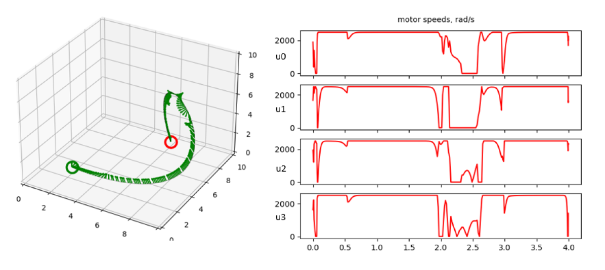
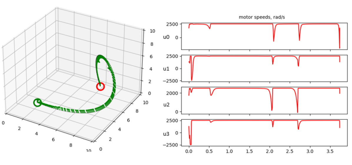
Figure 6: A sample trajectory computed with TOPPQuad for both a unidirectional (top) and bidirectional (bottom) quadrotor, and the respective motor speeds. The green vectors represent the quadrotor’s $\mathbf{R}\mathbf{e}_{3}$ vector at each point along the trajectory

V-D TOPPQuad in the Wild

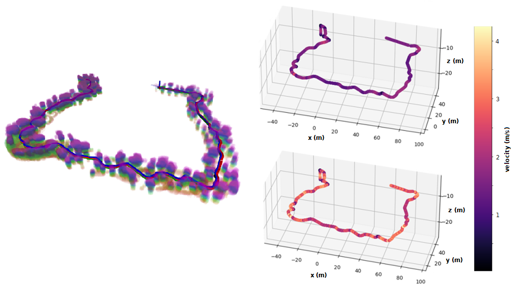
Figure 7: Obstacle-free path through a forest (Left) . We show the quadrotor speed along the original path (Top right) and refined TOPPQuad path (Top left). Maximum velocity is bounded at $v=5m/s$.

Finally, we demonstrate the performance of our planner on real-world data, when not all initial guess values are known. We apply TOPPQuad to a trajectory flown in the Wharton State Forest, NJ, USA, where a Falcon IV quadrotor autonomously navigated under the canopy of a large, tree-dense environment ([22], [23]). We recover the geometric path and the initial guess for TOPPQuad from the flight’s odometry data. As we do not have estimates of motor speeds or angular acceleration, we use the values of the hover configuration ($4108$ $rad/s$, $0$ $rad/s^{2}$). Fig. 7 shows the increase in speed along the obstacle-free path. The total trajectory time decreases from $236$ $sec$ to $136$ $sec$ across a total trajectory length of $336.2$ $m$.

VI Conclusion

We present TOPPQuad, an optimization algorithm for finding time-optimal quadrotor trajectories. We explicitly enforce state and input constraints, such as motor speeds, instead of relying on convex relaxations, which we demonstrate are not always sufficient. The key to our algorithm is an optimization of the total trajectory time given the full dynamics of the quadrotor. We show the ability to refine trajectories that come from a variety of commonly used flatness-based planners, expand motor speed bounds to automatically generate trajectories for bidirectional quadrotors, and demonstrate our planner’s performance on real world data.

However, our algorithm still has room for improvement time. Firstly, the computation time takes on the order of half a minute. Secondly, by virtue of solving a non-convex problem, our planner is not complete. However, fall-backs such as $\alpha$-scaling offer completeness, although without guarantees of time-optimality. Finally, our model does not account for drag or motor dynamics. Future work will focus on examining implementations for improving algorithm computation time and will focus on a higher fidelity model by incorporating representations of air resistance and motor dynamics into the optimization framework.

References

- [1] S. M. LaValle, “Planning algorithms.” Cambridge university press, 2006, ch. 14, pp. ”841–855”.
- [2] D. Mellinger and V. Kumar, “Minimum snap trajectory generation and control for quadrotors,” in 2011 IEEE international conference on robotics and automation. IEEE, 2011, pp. 2520–2525.
- [3] M. J. Van Nieuwstadt and R. M. Murray, “Real-time trajectory generation for differentially flat systems,” International Journal of Robust and Nonlinear Control: IFAC-Affiliated Journal, vol. 8, no. 11, pp. 995–1020, 1998.
- [4] M. Hehn and R. D’Andrea, “Real-time trajectory generation for quadrocopters,” IEEE Transactions on Robotics, vol. 31, no. 4, pp. 877–892, 2015.
- [5] C. Richter, A. Bry, and N. Roy, “Polynomial trajectory planning for aggressive quadrotor flight in dense indoor environments,” in Robotics Research: The 16th International Symposium ISRR. Springer, 2016, pp. 649–666.
- [6] S. Liu, K. Mohta, N. Atanasov, and V. Kumar, “Search-based motion planning for aggressive flight in se (3),” IEEE Robotics and Automation Letters, vol. 3, no. 3, pp. 2439–2446, 2018.
- [7] Z. Wang, X. Zhou, C. Xu, and F. Gao, “Geometrically constrained trajectory optimization for multicopters,” IEEE Transactions on Robotics, vol. 38, no. 5, pp. 3259–3278, 2022.
- [8] J. E. Bobrow, S. Dubowsky, and J. S. Gibson, “Time-optimal control of robotic manipulators along specified paths,” The international journal of robotics research, vol. 4, no. 3, pp. 3–17, 1985.
- [9] D. Verscheure, B. Demeulenaere, J. Swevers, J. De Schutter, and M. Diehl, “Time-optimal path tracking for robots: A convex optimization approach,” IEEE Transactions on Automatic Control, vol. 54, no. 10, pp. 2318–2327, 2009.
- [10] T. Lipp and S. Boyd, “Minimum-time speed optimisation over a fixed path,” International Journal of Control, vol. 87, no. 6, pp. 1297–1311, 2014.
- [11] H. Nguyen and Q.-C. Pham, “Time-optimal path parameterization of rigid-body motions: Applications to spacecraft reorientation,” Journal of Guidance, Control, and Dynamics, vol. 39, no. 7, pp. 1667–1671, 2016.
- [12] H. Pham and Q.-C. Pham, “A new approach to time-optimal path parameterization based on reachability analysis,” IEEE Transactions on Robotics, vol. 34, no. 3, pp. 645–659, 2018.
- [13] G. Ryou, E. Tal, and S. Karaman, “Multi-fidelity black-box optimization for time-optimal quadrotor maneuvers,” The International Journal of Robotics Research, vol. 40, no. 12-14, pp. 1352–1369, 2021.
- [14] P. Foehn, A. Romero, and D. Scaramuzza, “Time-optimal planning for quadrotor waypoint flight,” Science Robotics, vol. 6, no. 56, p. eabh1221, 2021.
- [15] L. Consolini, M. Locatelli, A. Minari, and A. Piazzi, “An optimal complexity algorithm for minimum-time velocity planning,” Systems & Control Letters, vol. 103, pp. 50–57, 2017.
- [16] I. Spasojevic, V. Murali, and S. Karaman, “Asymptotic optimality of a time optimal path parametrization algorithm,” IEEE Control Systems Letters, vol. 3, no. 4, pp. 835–840, 2019.
- [17] P. Virtanen, R. Gommers, T. E. Oliphant, M. Haberland, T. Reddy, D. Cournapeau, E. Burovski, P. Peterson, W. Weckesser, J. Bright, S. J. van der Walt, M. Brett, J. Wilson, K. J. Millman, N. Mayorov, A. R. J. Nelson, E. Jones, R. Kern, E. Larson, C. J. Carey, İ. Polat, Y. Feng, E. W. Moore, J. VanderPlas, D. Laxalde, J. Perktold, R. Cimrman, I. Henriksen, E. A. Quintero, C. R. Harris, A. M. Archibald, A. H. Ribeiro, F. Pedregosa, P. van Mulbregt, and SciPy 1.0 Contributors, “SciPy 1.0: Fundamental Algorithms for Scientific Computing in Python,” Nature Methods, vol. 17, pp. 261–272, 2020.
- [18] S. Diamond and S. Boyd, “CVXPY: A Python-embedded modeling language for convex optimization,” Journal of Machine Learning Research, vol. 17, no. 83, pp. 1–5, 2016.
- [19] J. A. E. Andersson, J. Gillis, G. Horn, J. B. Rawlings, and M. Diehl, “CasADi – A software framework for nonlinear optimization and optimal control,” Mathematical Programming Computation, vol. 11, no. 1, pp. 1–36, 2019.
- [20] W. Giernacki, M. Skwierczyński, W. Witwicki, P. Wroński, and P. Kozierski, “Crazyflie 2.0 quadrotor as a platform for research and education in robotics and control engineering,” in 2017 22nd International Conference on Methods and Models in Automation and Robotics (MMAR), 2017, pp. 37–42.
- [21] K. Mao, J. Welde, M. A. Hsieh, and V. Kumar, “Trajectory planning for the bidirectional quadrotor as a differentially flat hybrid system,” in 2023 IEEE International Conference on Robotics and Automation (ICRA), 2023, pp. 1242–1248.
- [22] L. Jarin-Lipschitz, X. Liu, Y. Tao, and V. Kumar, “Experiments in adaptive replanning for fast autonomous flight in forests,” in 2022 International Conference on Robotics and Automation (ICRA), 2022, pp. 8185–8191.
- [23] X. Liu, G. V. Nardari, F. C. Ojeda, Y. Tao, A. Zhou, T. Donnelly, C. Qu, S. W. Chen, R. A. F. Romero, C. J. Taylor, and V. Kumar, “Large-scale autonomous flight with real-time semantic slam under dense forest canopy,” IEEE Robotics and Automation Letters, vol. 7, no. 2, pp. 5512–5519, 2022.