Efficient homogenization of multicomponent metamaterials: chiral effects

Abstract

We extend an efficient homogenization procedure based on a Haydock representation of the microscopic wave operator for the calculation of the macroscopic dielectric response of a periodic composite to the case of an arbitrary number of components of arbitrary composition. As a test, we apply our numerical procedure to the calculation of the optical properties of a Bouligand structure, made of a large number of anisotropic layers stacked on top of each other and progresively rotated. This system consitutes a photonic crystal with circularly polarized electromagnetic normal modes, naturally ocurring in the cuticle of several arthropods, and which has a gap for one helicity, which corresponds to the observation of circularly polarized strong metallic like reflections. Our numerical procedure is validated through its good agreement with the analytical solution for this simple chiral system.

I Introduction

The importance of the optical properties of inhomogeneous artificial media such as metamaterials and photonic crystals made up of alternating particles of diverse ordinary materials has been well established. They have led to novel miniature optical devices [1]. Metamaterials may display exotic optical properties that are absent from ordinary materials such as a negative index of refraction [2]. These properties may me employed to design systems such as invisibility cloaks [3] based on metamaterials with permittivities and permeabilities that mimic the properties of curved space [4]. By manipulating the variation of the phase of a lightwave along a surface on which high index of refraction particles of appropiate shape, size and orientation are layed down, planar metalenses [5] can be fabricated. They may be designed to focus light with a high numerical aperture, to elliminate chromatic aberration [6], they may be tuned through mechanical stretching or controlled phase changes changes [7], and they may be sensitive to the polarization of light. For example, in Ref. [8] a submillimeter metasurface capable of focusing light of different wavelengths at pre-established points along a single focal plane was developed, leading to ultra-compact spectrometers.

One approach to the calculation of the optical properties of these systems is through the homogenization of its dielectric properties; the inhomogeneous system is replaced by a homogeneous material with effective properties related to its composition and geometry [9]. The most simple and widely used homogenization method is that of Maxwell-Garnett [10], based on the quasi-static interaction among small polarizable spherical particles within a host. Many other homogenization schemes have since been devised with a more general applicability. For example, in Ref. [11] a formulation of the bianisotropic macroscopic response of a metamaterial with an arbitrary composition and geometry was derived in the long-wavelength regime. A very general approach to the calculation of the macroscopic dielectric response of inhomogeneous materials, with some applications to liquids and disordered systems, roughnes at surfaces, periodic crystals and the surface local field effect was developed in Refs. [12, 13]. The formal theory therein has been further developed in the non-retarded limit [14], and led to the development of a very efficient numerical procedure, inspired on Haydock’s recursive procedure [15] for the calculation of the projected Green’s functions of quantum systems. That procedure is applicable to binary metamaterials made of arbitrary materials, dielectric or conducting, dispersive or not, dissipative or transparent, as it factors out the dynamical response of the components, which are encoded by a single number $u$, the possibly complex and frequency dependent spectral variable, from the geometry of the system which is characterized by a real characteristic function $B(\bm{r})$ of the position $\bm{r}$. The longitudinal component of the characteristic function is interpreted as a Hermitian operator, analogous to a Hamiltonian, and an iterative procedure yields its representation as a symmetric tridiagonal matrix whose elements are the Haydock coefficients. The macroscopic response is then given by a continued fraction in terms of the Haydock coefficients and the spectral variable. This procedure may be applied in one, two or three dimensions [14, 16], and it has been used to design and optimize thin devices to manipulate the polarization of light [17, 18]. Furthermore, the formalism allows the calculation of the microscopic electric field, and from it, nonlinear processes such as interface induced second harmonic generation [19]. The theory was generalized to the calculation of the macroscopic response of periodic binary materials in the retarded regime, in which the period of the structure is comparable to the wavelength of light [20]. In this work it was shown that the concept of a homogenized response does make sense even in the retarded regime, and that the macroscopic wave equation may be employed to obtain the photonic band structure of the system. However, to that end, the spatial dispersion or non-locality of the macroscopic permittivity has to be accounted for. Nonlocality has been shown to be important for the description of the response of nanometric metallic components [21]. Furthermore, non-locality of the effective response may be useful for the design of novel elements such as broadband, omnidirectiona impedance matching layers [22]. From the non-local dependance of the macroscopic response on the wave-vector $\bm{k}$, beyond its dependence on the frequency $\omega$, the magnetic properties of metamaterials made of non-magnetic materials may be extracted [23] in accordance to the Landau-Lifshitz approach [24].

A limitation of the homogenization procedure above is that it is constrained to binary metamaterials, made of only two components. The reason is that the geometry of the system is described by a characteristic function $B(\bm{r})$ that takes only two values, 0 and 1, depending on the material that occupies the position $\bm{r}$. The theory may readily be generalized to metamaterials with more components by renouncing to the factorization into geometry and dynamics, by writing the theory in terms of the position dependent microscopic response $\epsilon(\bm{r})$. However, the need for a Hermitian operator analogous to a Hamiltonian in order to apply Haydock’s formalism would restrict the formalism to media free of dissipation. In Ref. [25] it was noted that using an Euclidean internal product of wavefunctions instead of the usual Hermitian product, the relevant operators such as the dielectric response and its longitudinal proyection become symmetric in an extended space, in which counterpropagating waves, with wavevectors $\pm\bm{k}$ are considered simultaneously. As symmetric operators share many of their properties with Hermitian operators, it was possible to reformulate Haydock’s formalism for the calculation of the macroscopic response of multicomponent metamaterials of arbitrary composition and with an arbitrary number of components. Nevertheless, that formulation was restricted to the non-retarded regime.

The purpose of the present paper is to formulate the calculation of the macroscopic response of multicomponent metamaterials of arbitrary composition by applyingd the ideas developed in Ref. [25] to the retarded formulation developed in Ref. [20].

The structure of the paper is the following: In Sec. II we develop the theory. In order to test the theory, in Sec. III we apply it to a simple system, a Bouligand structure [26, 27], such as that present in the cuticles of several arthropods, and consisting of chitin micro-filaments that are arranged in layers within which the filaments are aligned, but rotated with respect to the filaments in the layers above and below, making an helicoidal structure analogous to that within cholesteric liquid crystals. The system is interesting as it is a naturaly ocurring photonic crystal whose optical properties include iridescent metalic-like reflections that furthermore, produce circularly polarized light. To perform the calculation we have extended the computational package Photonic [28] to incorporate the results of Sec. II, and we used it to obtain the macroscopic non-local response, analyze its structure and obtain the dispersion relation of the normal modes. In order test our numerical results, in Sec. IV we develop an exact analytical theory to obtain the macroscopic dielectric tensor and the normal modes of the system, and we explain their features such as optical activity and photonic band structure. Finally, Sec. V is devoted to conclusions.

II Theory

Following Ref. [20], from Maxwell’s equations we find an integral equation for the electric field $\bm{E}$ within the metamaterial, which we write formally as

$$\bm{E}=-\hat{\mathcal{W}}^{-1}\frac{4\pi i}{qc\epsilon_{h}}\bm{j}^{\text{ex}},$$ (1)

where $\bm{j}^{\text{ex}}$ is an external monochromatic current source oscillating in time with frequency $\omega$ and in space with some given wavevector $\bm{k}$, $q=\omega/c$ is the free-space wave-number corresponding to $\omega$, $\epsilon_{h}$ is an arbitrary convenient reference position independent permittivity, and $\hat{\mathcal{W}}$ is the wave operator

$$\hat{\mathcal{W}_{ij}}=\frac{\hat{\epsilon}^{ij}}{\epsilon_{h}}-\frac{\partial_{i}\partial_{j}-\delta_{ij}\nabla^{2}}{\epsilon_{h}q^{2}},$$ (2)

with $\hat{\bm{\epsilon}}$ the microscopic dielectric operator corresponding to the position dependent local permittivity $\bm{\epsilon}(\bm{r})$, which may be a scalar or a tensor with real or complex frequency dependent components, $\partial_{i}$ denotes the partial derivative with respect to the spatial coordinate $r_{i}$ ($i=$1,2,3 or $x,y,z$), and $\delta_{ij}$ is Kronecker’s delta. As the source $\bm{j}^{\text{ex}}$ is unrelated to the induced currents due to the response $\hat{\bm{\epsilon}}$, it has no spatial fluctuations [12] related to the texture of the metamaterial, so it is equal to its average

$$\bm{j}_{M}^{\text{ex}}=\bm{j}_{a}^{\text{ex}}=\hat{\mathcal{P}}_{a}\bm{j},$$ (3)

where we denote macroscopic quantities by the index $M$ and we introduce the average operator $\hat{\mathcal{P}}_{a}$, which together with the fluctuation operator ${\mathcal{P}}_{f}=\hat{1}-\hat{\mathcal{P}}_{a}$ forms a couple of complementary idempotent projectors, $\hat{\mathcal{P}}_{a}\hat{\mathcal{P}}_{a}=\hat{\mathcal{P}}_{a}$, $\hat{\mathcal{P}}_{f}\hat{\mathcal{P}}_{f}=\hat{\mathcal{P}}_{f}$, $\hat{\mathcal{P}}_{a}\hat{\mathcal{P}}_{f}=\hat{\mathcal{P}}_{f}\hat{\mathcal{P}}_{a}=0$. Thus, averaging Eq. (1) we obtain

$$\bm{E}_{M}=-\hat{\mathcal{W}}_{M}^{-1}\frac{4\pi i}{qc\epsilon_{h}}\bm{j}^{\text{ex}},$$ (4)

where we identify the macroscopic inverse wave operator

$$\hat{\mathcal{W}}_{M}^{-1}=\hat{\mathcal{P}}_{a}\hat{\mathcal{W}}^{-1}\hat{\mathcal{P}}_{a},$$ (5)

that is, the inverse macroscopic wave operator is the average of the inverse of the microscopic wave operator restricted to act on averaged sources. From the macroscopic wave operator one can extract the macroscopic dielectric tensor and employ it to calculate the optical properties of the system.

In Ref. [20] the microscopic wave operator of a binary system was written in terms of a Hermitian operator which was built from the characteristic function that defined the geometry of the system, and its use allowed the use of Haydock’s recursion to obtain a tri-diagonal representation of $\hat{\mathcal{W}}$, from which the macroscopic response was readily obtained. However, for multicomponent systems that procedure may not be directly applied, and the presence of dissipation disallows to use directly the non-Hermitian wave operator within Haydock’s scheme. Our purpose is to obtain a procedure that may be applied to multicomponent systems of arbitrary geometry and composition. Thus, it must be capable to deal with dissipation. In Ref. [25] a similar problem was solved by redefining the inner product of two fields. Instead of the usual Hermitian product

$$\braket{\psi}{\phi}=\frac{1}{V}\int d^{3}r\,\psi^{*}(\bm{r})\phi(\bm{r})\quad\text{(Hermitian)}$$ (6)

between two states $\ket{\psi}$ and $\ket{\phi}$ corresponding to the scalar wavefunctions $\psi(\bm{r})$ and $\psi(\bm{r})$ within a volume $V$, we introduce the Euclidean product

$$\braket{\psi}{\phi}=\frac{1}{V}\int d^{3}r\,\psi(\bm{r})\phi(\bm{r}),\quad\text{(Euclidean)}$$ (7)

notwithstanding the fact that for complex valued fields it is not positive definite and it may produces complex values for the product of a state with itself. The generalization to vector valued states is immediate. The motivation for using this product is that the matrix elements of the wave operator between any two vector valued states $\ket{\bm{\psi}}$ and $\ket{\bm{\phi}}$ represented in real space by the functions $\psi_{i}(\bm{r})$ and $\phi_{i}(\bm{r})$, and in reciprocal space by the Fourier transforms $\psi_{i}(\bm{p})$ and $\phi_{i}(\bm{p})$, where $\bm{p}$ is the wavevector, is

$$\braket{\bm{\psi}}{\hat{\mathcal{W}}}{\bm{\phi}}=\int d^{3}p^{\prime}\int d^{3}p\,\psi_{i}(\bm{p}^{\prime})\left(\frac{\epsilon^{ij}(-\bm{p}^{\prime}-\bm{p})}{\epsilon_{h}}-\delta(\bm{p}^{\prime}+\bm{p})\frac{p^{2}\delta_{ij}-p_{i}p_{j}}{\epsilon_{h}q^{2}}\right)\phi_{j}(\bm{p}),$$ (8)

where we apply Einstein implicit sumation convention to the repeated cartesian indices $i$ and $j$ (disregarding if they are subscripts or superscripts), $\epsilon^{ij}(-\bm{p}^{\prime}-\bm{p})$ is the Fourier transform of $\epsilon^{ij}(\bm{r})$ with wavevector $\bm{p}^{\prime}-\bm{p}$ and $\delta(\ldots)$ is Dirac’s delta. Notice that the interchange $\ket{\bm{\psi}}\leftrightarrow\ket{\bm{\phi}}$ leaves the matrix element invariant. This means that under this product the wave operator is symmetric, i.e., it has symmetric matrix elements between any pair of states. There are important theorems about real symmetric linear operators that are analogous to those for Hermitian operators, and some of them may be carried over to complex symmetrical matrices. This allows generalizing Haydock’s procedure to complex symmetrical matrices.

To proceed, we assume that the system is periodic in space. Thus, $\epsilon^{ij}(-\bm{p}-\bm{p}^{\prime})$ is null unless $\bm{p}+\bm{p}^{\prime}$ is a reciprocal vector of the lattice. Writing $\bm{p}=\bm{k}+\bm{G}\equiv\bm{G}_{\bm{k}}$, then the only relevant value for $\bm{p}^{\prime}$ are of the form $\bm{p}^{\prime}=-\bm{k}-\bm{G}^{\prime}=-\bm{G}^{\prime}_{\bm{k}}$, where $\bm{k}$ is a Bloch’s vector and $\bm{G}$ and $\bm{G}^{\prime}$ are reciprocal vectors, and we may rewrite Eq. (8) as

$$\braket{\bm{\psi}}{\hat{\mathcal{W}}}{\bm{\phi}}=\int_{BZ}d^{3}k\sum_{\bm{G}^{\prime}}\sum_{\bm{G}}\psi_{i,-\bm{G}^{\prime}_{\bm{k}}}\left(\frac{\epsilon^{ij}_{\bm{G}^{\prime}-\bm{G}}-\bm{G}_{\bm{k}}^{2}(\mathcal{P}^{T}_{\bm{G}^{\prime}\bm{G}}(\bm{k}))_{ij}}{\epsilon_{h}q^{2}}\right)\phi_{j,{\bm{G}_{\bm{k}}}},$$ (9)

where $\bm{\epsilon}_{\bm{G}^{\prime}-\bm{G}}$ is the coefficient of the Fourier series of $\bm{\epsilon}(\bm{r})$ corrersponding to the reciprocal vector $\bm{G}^{\prime}-\bm{G}$,

$$(\mathcal{P}^{T}_{\bm{G}^{\prime}\bm{G}}(\bm{k}))_{ij}=\delta_{\bm{G}^{\prime},\bm{G}}\delta_{ij}-(\mathcal{P}^{L}_{\bm{G}\bm{G}^{\prime}}(\bm{k}))_{ij}$$ (10)

is the transverse projector for a wave with wavevector $\bm{G}_{\bm{k}}\equiv\bm{k}+\bm{G}$, and

$$(\mathcal{P}^{L}_{\bm{G}^{\prime}\bm{G}}(\bm{k}))_{ij}=\delta_{\bm{G}^{\prime},\bm{G}}\frac{(\bm{G}_{\bm{k}})_{i}(\bm{G}_{\bm{k}})_{j}}{(\bm{k}+\bm{G})^{2}}$$ (11)

is the longitudinal projector. Notice that in this expressions a Bloch’s vector $\bm{k}$ is only coupled to $-\bm{k}$ and viceversa, so we can restrict ourselves to states consisting of two counterpropagating Bloch waves ($\pm$) with fixed Bloch vectors $\pm\bm{k}$ and thus eliminate the integral over the Brillouin zone (BZ) in Eq. (9). We write such pair of states employing a spinor like notations in terms of 2-vectors

$$\ket{\bm{\phi}}\to\begin{pmatrix}\bm{\phi}_{+,\bm{G}}\\ \bm{\phi}_{-,\bm{G}}\\ \end{pmatrix},$$ (12)

each of whose components is a vector field that depends on the reciprocal vectors $\bm{G}$, with corresponding inner product

$$\braket{\bm{\psi}}{\bm{\phi}}=\sum_{\bm{G}}(\bm{\psi}_{-,-\bm{G}}\cdot\bm{\phi}_{+,\bm{G}}+\bm{\psi}_{+,-\bm{G}}\cdot\bm{\phi}_{-,\bm{G}}).$$ (13)

The wave operator in this space may then be be represented as a $2\times 2$ matrix

$$\mathcal{W}_{\bm{G}\bm{G}^{\prime}}=\begin{pmatrix}\frac{\bm{\epsilon}_{\bm{G}-\bm{G}^{\prime}}}{\epsilon_{h}}-\frac{\bm{G}_{\bm{k}}^{2}\mathcal{P}^{T}_{\bm{G}\bm{G}^{\prime}}(\bm{k})}{\epsilon_{h}q^{2}}&0\\ 0&\frac{\bm{\epsilon}_{\bm{G}-\bm{G}^{\prime}}}{\epsilon_{h}}-\frac{\bm{G}_{-\bm{k}}^{2}\mathcal{P}^{T}_{\bm{G}\bm{G}^{\prime}}(-\bm{k})}{\epsilon_{h}q^{2}}\end{pmatrix}$$ (14)

In order to tame the growth of $\mathcal{W}$ with $\bm{G}$ it is convenient to rewrite (14) as

$$\hat{\mathcal{W}}=(\hat{\bm{1}}-\hat{\bm{H}}\hat{\bm{g}})\hat{\bm{g}}^{-1},$$ (15)

where the inverse of the operator $\hat{\bm{g}}$ is

$${\bm{g}}^{-1}_{\bm{G}^{\prime}\bm{G}}=\begin{pmatrix}\bm{1}-\frac{G_{\bm{k}}^{2}}{\epsilon_{h}q^{2}}\mathcal{P}^{T}_{\bm{G}\bm{G}}(\bm{k})&0\\ 0&\bm{1}-\frac{G_{-\bm{k}}^{2}}{\epsilon_{h}q^{2}}\mathcal{P}^{T}_{\bm{G}\bm{G}}(-\bm{k}),\\ \end{pmatrix}\delta_{\bm{G}^{\prime}\bm{G}}$$ (16)

where $\bf 1$ is the cartesian unit matrix, while

$$\hat{\bm{H}}=\frac{\epsilon_{h}\hat{\bm{1}}-\hat{\bm{\epsilon}}}{\epsilon_{h}}.$$ (17)

Notice that $\hat{\bm{H}}$ and $\hat{\bm{g}}$ correspond to symmetric operators, but not so their product $\hat{\bm{H}}\hat{\bm{g}}$. Nevertheless, introducing yet another inner product,

$$(\bm{\psi}|\bm{\phi})=\braket{\bm{\psi}}{\hat{\bm{g}}}{\bm{\phi}}$$ (18)

interpeting $\hat{\bm{g}}$ as a metric, the operator $\hat{\bm{H}}\hat{\bm{g}}$ becomes symmetric, i.e., $(\bm{\psi}|\hat{\bm{H}}\hat{\bm{g}}|\bm{\phi})=\braket{\bm{\psi}}{\hat{\bm{g}}\hat{\bm{H}}\hat{\bm{g}}}{\bm{\phi}}=\braket{\bm{\phi}}{\hat{\bm{g}}\hat{\bm{H}}\hat{\bm{g}}}{\bm{\psi}}=(\bm{\phi}|\hat{\bm{H}}\hat{\bm{g}}|\bm{\psi})$ for any pair of spinor states $\ket{\bm{\psi}}$ and $\ket{\bm{\phi}}$. The metric $\hat{\bm{g}}$ is readily obtained from Eq. (16), and it is a diagonal matrix in reciprocal space with elements

$$\bm{g}_{\bm{G}^{\prime}\bm{G}}=\begin{pmatrix}\frac{\epsilon_{h}q^{2}\bm{1}-G_{\bm{k}}^{2}{\mathcal{P}}^{L}_{\bm{G}\bm{G}}(\bm{k})}{\epsilon_{h}q^{2}-G_{\bm{k}}^{2}}&0\\ 0&\frac{\epsilon_{h}q^{2}\bm{1}-G_{-\bm{k}}^{2}{\mathcal{P}}^{L}_{\bm{G}\bm{G}}(-\bm{k})}{\epsilon_{h}q^{2}-G_{-\bm{k}}^{2}}\end{pmatrix}\delta_{\bm{G}^{\prime}\bm{G}},.$$ (19)

To calculate the inverse macroscopic wave operator,

$$\hat{\mathcal{W}}_{M}^{-1}=\hat{\mathcal{P}}_{a}\hat{\bm{g}}(\hat{\bm{1}}-\hat{\bm{H}}\hat{\bm{g}})^{-1}\hat{\mathcal{P}}_{a},$$ (20)

we start by defining a normalized macroscopic starting state $\ket{\bm{\phi}_{0}}$, a spinor consisting of two counterpropagating plane waves with wavevectors $\pm\bm{k}$, with corresponding polarizations $\hat{\bm{e}}_{\pm}$ and normalized so that

$$\braket{\bm{\phi}_{0}}{\bm{\phi}_{0}}=1.$$ (21)

Then, we start Haydock’s iteration with the same state but normalized according to the metric $\hat{\bm{g}}$,

$$\ket{0}=\frac{1}{b_{0}}\ket{\bm{\phi}_{0}},$$ (22)

where

$$b_{0}^{2}=\braket{\bm{\phi}_{0}}{\hat{\bm{g}}}{\bm{\phi}_{0}}.$$ (23)

Starting from $\ket{0}$ and defining $\ket{-1}\equiv 0$, we define iteratively the states $\ket{n}$ through the Haydock recursion

$$b_{n+1}\ket{n+1}=\hat{\bm{H}}\hat{\bm{g}}\ket{n}-a_{n}\ket{n}-b_{n}\ket{n-1},$$ (24)

where the coefficients $a_{n}$ and $b_{n+1}$ are chosen so that the state $\ket{n+1}$ is orthogonal to all previous states and is itself normalized, i.e.,

$$\braket{n}{\hat{\bm{g}}}{m}=\delta_{nm}.$$ (25)

Due to the symmetry of $\hat{\bm{H}}\hat{\bm{g}}$, the coefficient of $\ket{n-1}$ in Eq. (24) is simply the coefficient $b_{n}$ obtained in the previous step, and there is no contribution from states $\ket{n-2}$, $\ket{n-3}$, etc. Notice that in this basis the wave operator is represented by a tridiagonal symmetric matrix

$$(\mathcal{W}_{nm})=\begin{pmatrix}1-a_{0}&-b_{1}&0&0&\cdots\\ -b_{1}&1-a_{1}&-b_{2}&0&\cdots\\ 0&-b_{2}&1-a_{2}&-b_{3}&\cdots\\ \vdots&\vdots&\vdots&\vdots&\ddots\end{pmatrix}$$ (26)

though its entries are in general complex numbers. The projected inverse wave operator is then given by a continued fraction,

$$\braket{\phi_{0}}{\mathcal{W}^{-1}}{\phi_{0}}=b_{0}^{2}\braket{0}{\mathcal{W}^{-1}}{0}=\frac{b_{0}^{2}}{1-a_{0}-\frac{b_{1}^{2}}{1-a_{1}-\frac{b_{2}^{2}}{1-a_{2}-\ddots}}}-$$ (27)

From Eqs. (12), (13) and (20), we interpret the result above as $\hat{\bm{e}}_{-}\cdot(\mathcal{W}_{M}^{-1})_{++}\cdot\hat{\bm{e}}_{+}+\hat{\bm{e}}_{+}\cdot(\mathcal{W}_{M}^{-1})_{--}\cdot\hat{\bm{e}}_{-}$, where $\pm$ denote spinor indices. Thus, repeating the calculation for different polarization vectors $\hat{\bm{e}}_{\pm}$ such as $\hat{\bm{e}}_{+}=\hat{\bm{x}}$, $\hat{\bm{y}}$, $(\hat{\bm{x}}+\hat{\bm{y}})/\sqrt{2}$, $(\hat{\bm{x}}+i\hat{\bm{y}})/\sqrt{2}$, etc., with $\hat{\bm{e}}_{-}=\hat{\bm{e}}_{+}^{*}$, and using the condition of symmetry under the simultaneous reversal of Bloch’s vector $\bm{k}\leftrightarrow-\bm{k}$, and interchange of cartesian indices $i\leftrightarrow j$, we may obtain all the components of $\mathcal{W}_{M}^{-1}$. A simple matrix inversion yields then the macroscopic wave operator, which we interpret using Eq. (14) in terms of the macroscopic dielectric tensor as

$$(\mathcal{W}_{M})_{++}=\frac{\bm{\epsilon}^{M}(\bm{k})}{\epsilon_{h}}-\frac{k^{2}\mathcal{P}^{T}_{\bm{0}\bm{0}}(\bm{k})}{\epsilon_{h}q^{2}}.$$ (28)

The procedure above and some others have been incorporated into a free, open access computational package called Photonic written in the Perl language and using the Perl Data Language number-crunching extension and is available in a Github repository [28].

III Application

To test the theory developed in the previous section and its numerical implementation we use a simple multicomponent system given by a Bouligand structure. This kind of structures is present in the cuticle of several arthropods [26, 27] and sometimes it is responsible for strong metallic-like reflections which are frequently iridescent and which furthermore are circularly polarized. The structures consist of stacked layers, each of which consists of fibers of chitin, a protein, aligned along the layer and giving rise to an anisotropic thin film. Subsequent films are stacked one over the other rotated among themselves around the stacking axis giving rise to a helical structure as illustrated in Fig. 1, similar to that of cholesteric liquid crystals.

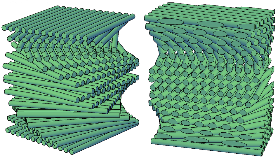
Figure 1: Bouligand structure. Films made of aligned fibers are stacked one on top of the other after a relative rotation by a constant angle. The left (right) side illustrates a left (right) helical structure. (Illustration by Andrea López-Reyna.)

Recently, the optical properties of individual layers was investigated using a homogenization procedure, and those of the full structure using a transfer matrix approach [30]. In this section we will apply the theory developed in the previous section to obtain the macroscopic response of Bouligand-like structures.

Notice that the system is periodic as it repeats itself after half a rotation. Thus, the modes of the system are Bloch waves. For simplicity, we will consider only Bloch waves moving along the stacking direction $\hat{\bm{s}}$. We assume that each layer has a well defined local dielectric response, which would be anisotropic. The principal axes of the layer’s response would naturally be the common axis of the fibers $\hat{\bm{f}}$, the normal $\hat{\bm{n}}=\hat{\bm{s}}\times\hat{\bm{f}}$ to the both fibers and to the stacking direction, and $\hat{\bm{s}}$, which we assume coincides with the $z$ axis. Thus, in these principal axes, the dielectric tensor would be

$$\bm{\epsilon}_{p}=\begin{pmatrix}\epsilon_{ff}&0&0&\\ 0&\epsilon_{nn}&0\\ 0&0&\epsilon_{zz}\end{pmatrix}=\begin{pmatrix}I+A&0&0\\ 0&I-A&0\\ 0&0&\epsilon_{zz}\end{pmatrix},$$ (29)

where we introduced the isotropic $I$ and anisotropic $A$ contributions to the in-plane response.

The dielectric response of a given layer at height $z$ may be obtained by rotating the response above by an angle $\theta$, which grows with $z$. Assuming that at $z=0$ $\hat{\bm{f}}$ points along $\hat{\bm{x}}$, we write $\theta(z)=G_{0}z$ where $G_{0}=\pm 2\pi/a$ with $a$ the pitch of the helix, i.e., the distance required for a full turn, and the sign of $G_{0}$ is positive (negative) for right (left) helices. Thus, the actual dielectric tensor at height $z$ would be

$$\bm{\epsilon}(z)=\bm{R}(z)\bm{\epsilon}_{p}\bm{R}^{T}(z),$$ (30)

where

$$\bm{R}(z)=\begin{pmatrix}\cos G_{0}z&-\sin G_{0}z&0\\ \sin G_{0}z&\cos G_{0}z&0\\ 0&0&1\end{pmatrix}$$ (31)

is a rotation matrix. Confining our attention to the in-plane response, the result is

$$\bm{\epsilon}(z)=I\begin{pmatrix}1&0\\ 0&1\\ \end{pmatrix}+A\begin{pmatrix}\cos 2G_{0}z&\sin 2G_{0}z\\ \sin 2G_{0}z&-\cos 2G_{0}z\end{pmatrix},$$ (32)

a height independent term propoprtional to the identity and a term that changes sinusoidally with a spatial period $a/2$ corresponding to a reciprocal vector $2G_{0}$.

To test the procedure detailed in the preceeding section we performed a numerical calculation using the Photonic package [28], assuming a unit cell consisting of $N>2$ layers numbered $n=0\ldots N-1$, of equal width $d$. The $n$-th layer is located at a height $z_{n}=nd$ and is rotated by an angle $\theta_{n}=G_{0}nd$, and thus has a dielectric tensor $\bm{\epsilon}_{n}=\bm{\epsilon}(nd)$ (Eq. (32)) that differs from that of other layers due to its different orientation. In the upper panel of Fig. 2 we show the diagonal component of the numerically calculatted macroscopic permitivity $\epsilon^{M}_{xx}(\omega,\bm{k})$ which equals $\epsilon^{M}_{yy}(\omega,\bm{k})$ as a function of the wavevector $\bm{k}=k\hat{\bm{z}}$ for a fixed frequency $\omega=c/a$ for a right handed Bouligand system with isotropic contribution to the microscopic permittivity $I=1.5$ and anisotropic contribution $A=0.5$.

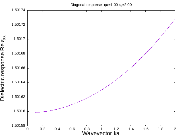
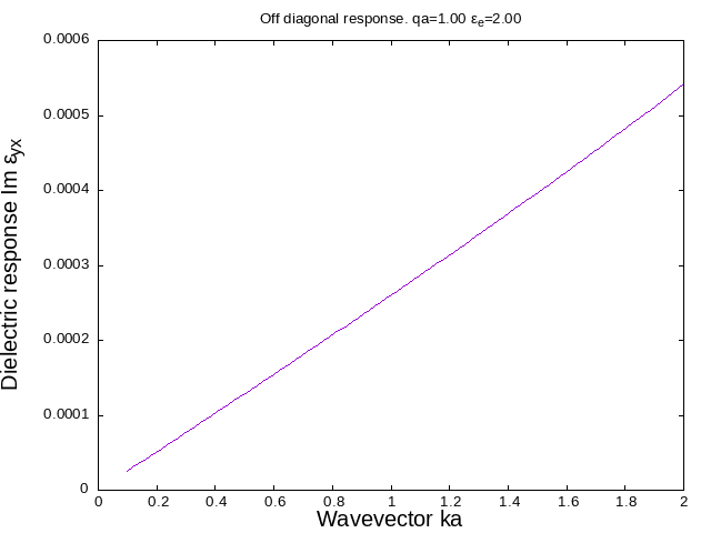
Figure 2: Diagonal components $\epsilon^{M}_{xx}(\omega,\bm{k})=\epsilon^{M}_{yy}(\bm{k},\omega)$ (top) and imaginary part of the offdiagonal components $\epsilon^{M}_{yx}=-\epsilon^{M}_{xy}$ (bottom) of the macroscopic permitivity as a function of the wavevector $\bm{k}=k\hat{\bm{z}}$ for a system with $N=11$ anisotropic layers per revolution with $I=1.5$, $A=0.5$, and frequency $\omega=c/a$

The results are already well converged for $N=11$ and using only 11 pairs of Haydock coefficients but much larger $N$’s may be used to better approximate a continuosly rotating helix. A non-retarded calculation would trivially yield an in-plane macroscopic response equal to the average over all the layers, that is $\bm{\epsilon}^{M}=I\hat{\bm{1}}$. Our results show a small deviation at $k=0$ due to the finite frequency and an additional small quadratic deviation $\propto k^{2}$ for small $k$. This quadratic dependence on the wavevector is a non-local effect than may be interpreted in terms of an effective magnetic response of the spatially dispersive system [23]. As the system has no dissipation, its diagonal response is real.

In Fig. 2 we also show the non-diagonal macroscopic response $\epsilon^{M}_{yx}$ (lower panel) for the same system as in Fig. 2, which turns out to imaginary, linear in $k$ for small $k$ and opposite to $\epsilon^{M}_{xy}$, so that in the absence of dissipation $\bm{\epsilon}^{M}$ is a Hermitian matrix.

Notice that the fact that the offdiagonal components of the permittivity tensor turned out to be antisymmetric does not contradict the statement in the previous section that with the Euclidean metric the matrix elements of the wave operator and related operators are symmetric, as the symmetry operation corresponds to an exchange of Cartesian indices $i\leftrightarrow j$ and a change of sign of the wavevector $\bm{k}\leftrightarrow-\bm{k}$ as stated in the previous section. Thus, the symmetric part of $\bm{\epsilon}^{M}$ should be an even function of the wavevector and its antisymmetric part should be an odd function. The quadratic and linear behaviors shown in Fig. 2 confirm this behaviour. Furthermore, in the absence of dissipation, $\bm{\epsilon}^{M}$ should be Hermitian. Thus, its symmetric part should be real and its antisymmetric part should be imaginary. Off-diagonal imaginary antisymmetric contributions to the response are an indication of optical activity [31], as could have been expected for Bouligand structures due to their chiral geometry.

The results above correspond to frequencies and wavevectors that are small with respect to the spatial period of the system. In Figs. 3 we show the equivalent results for a larger frequency $\omega=6c/a$ and a larger wavevector range $0<k<12/a$. Notice that both diagonal and off-diagonal components have a resonance above $k\approx 5/a$.

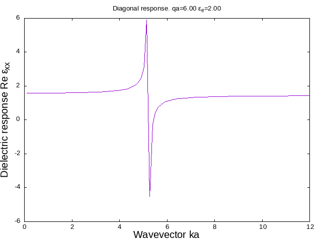
Figure 3: Diagonal (top) and off-diagonal (bottom) macroscopic response for the same system as in Fig. 2, but for a larger frequency $\omega=6c/a$ and larger wavevectors.

The normal modes of the structure may be obtained from the macroscopic wave equation in the absence of sources,

$$k^{2}\bm{E}=q^{2}\bm{\epsilon}^{M}(\omega,\bm{k})\bm{E},$$ (33)

which shows that $k^{2}/q^{2}$ should be an eigenvalue of the macroscopic dielectric tensor $\bm{\epsilon}^{M}(\omega,\bm{k})$. Given the shape of the in plane projection $\bm{\epsilon}^{M}$, a real multiple of the identity plus an imaginary antisymmetric matrix, its eigenvalues are of the form $\text{Re}\,\epsilon_{xx}\pm\text{Im}\epsilon_{yx}$, corresponding to right circular polarization, with $\bm{E}\propto(1,i)$, or left circular polarization, with $\bm{E}\propto(1,-i)$, as seen from the $z$ axis looking downward towards the $xy$ plane. Notice that with this convention, a wave with right (left) circular polarizatin would have positive (negative) helicity if it propagates in the $z$ direction and a negative (positive) helicity if it propagates in the $-z$ direction.

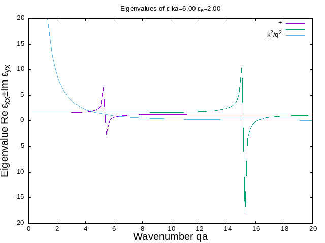
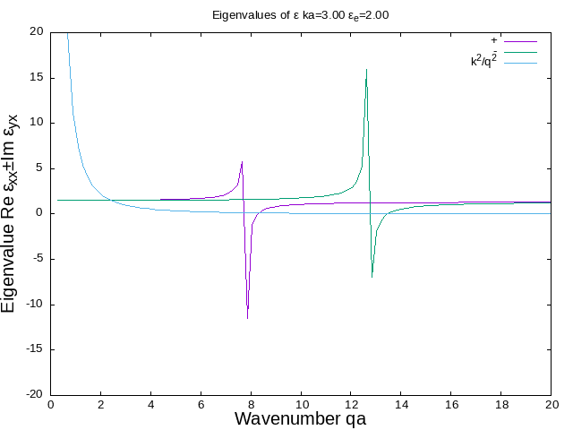
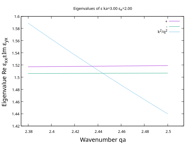
Figure 4: Eigenvalues of $\bm{\epsilon}^{M}$ for right ($+$) and left ($-$) circular polarizations and for different values $k=6/a$ (top panel) and $k=3/a$ (middle and bottom panels) of the wavevector, as a function of frequency $\omega=qc$. Also shown are the corresponding values of $k^{2}/q^{2}$. The right panel is a detail of the central panel.

The only difficulty for solving the dispersion relation (33) is that the eigenvalues depend on $\bm{k}$ due to spatial dispersion. In Fig. 4 we show the eigenvalues of $\bm{\epsilon}^{M}$ for the two circular polarizations and for two values of $k$. We also show a plot of $k^{2}c^{2}/\omega^{2}$. Its intersection with the eigenvalues yields the frequency $\omega(\bm{k})$ for the chosen wavevector $\bm{k}$ and polarization. The procedure could be repeated for several wavevectors to obtain the full dispersion relation.

Instead of searching for the intersections above, we can visualize the normal modes by plotting the determinant of the Green’s function corresponding to the macroscopic wave operator, $\det\mathcal{W}_{M}^{-1}(\omega,k)$, as the modes correspond to the singularities of the wave operator. For visualization purposes, we bound the poles of the Green’s function by introducing some dissipation, adding an imaginary part to the diagonal part of the microscopic response. This illustrates the fact that our procedure is able indeed to deal with dissipative multicomponent systems. The results are shown in the top panel of Fig. 5.

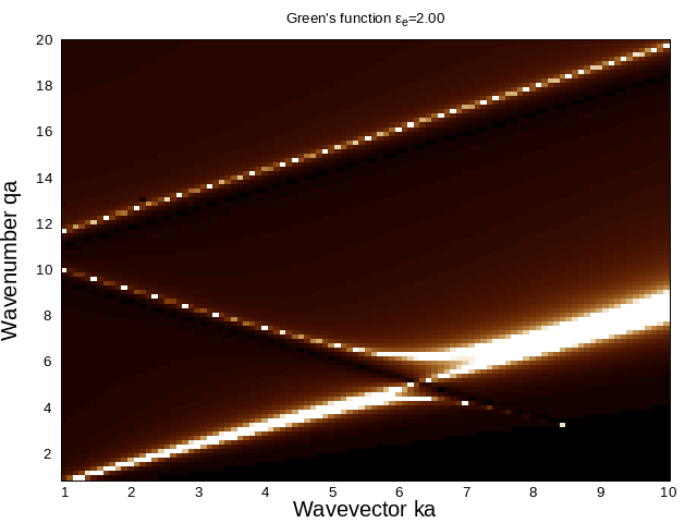
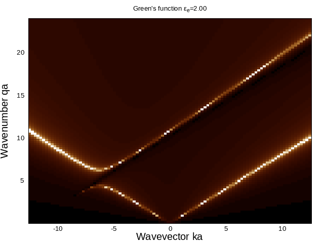
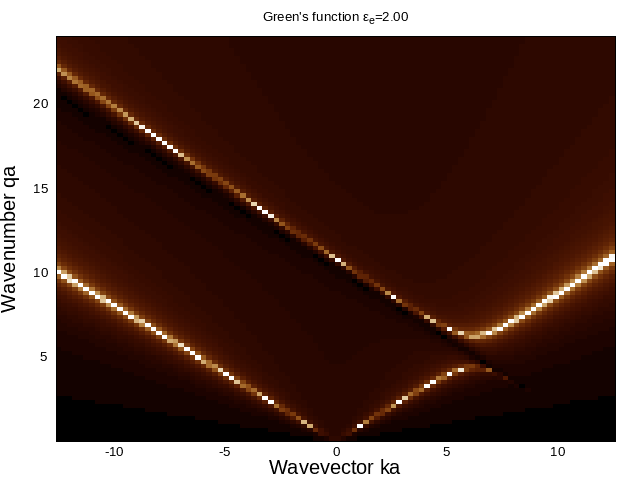
Figure 5: Determinant of the macroscopic inverse wave operator $\det\mathcal{W}_{M}^{-1}$ for the same system as in Fig. 2 as a function of frequency $\omega$ and wavevector $\bm{k}=k\hat{\bm{z}}$ (top panel). To bound the singularities, an imaginary part was added to the dielectric function. $\det\mathcal{W}_{M}^{-1}$ projected into right and left circular polarized states (middle and bottom panels).

A rich photonic band structure corresponding to the singularities of $\mathcal{W}_{M}$ may be observed. Its interpretation becomes simpler by projecting the Green’s function into right and left circular polarizations. Notice that there are photonic gaps at $k=\pm G_{0}$, the boundary of the 1D Brillouing zone, for which waves with negative helicity may not propagate within the structure. Accordingly, we expect a strong reflectance in a finite Bouligand structure at the corresponding frequencies. It is interesting to note that in this system there is negligible contrast between the response of adjacent layers; they have the same composition and they only differ by a small rotation. Nevertheless, the system is periodic and therefore it develops a photonic structure with allowed and forbidden bands. Furthermore, the dispersion relation for a given rotation sense is not symmetric under reversal of the propagation direction (for a given helicity it is symmetric).

IV Analytical results

In the previous section we obtained the macroscopic response and the normal modes of a Bouligand structure by using a general purpose theory developed for structures with an arbitrary number of different components of arbitrary geometry and composition, and employing its numerical implementation. Nevertheless, to test the validity of the results, it is important to compare them with those of alternative approaches. In this section we develop an analytical solution of the simple structure studied in section III and compare the results of both approaches.

Consider a circularly polarized plane wave propagating along $z$ with in-plane field

$$\bm{E}_{k\sigma}(z)=\frac{E_{k\sigma}}{\sqrt{2}}\begin{pmatrix}1\\ \sigma i\end{pmatrix}e^{ikz},$$ (34)

where $\sigma=1$ (-1) for right (left) circular polarization. Its interaction with a continuously rotating Bouligand structure described by the response given by Eq. (32) yields

$$\bm{\epsilon}\bm{E}_{k\sigma}(z)=I\bm{E}_{k\sigma}e^{ikz}+A\frac{E_{k\sigma}}{\sqrt{2}}\begin{pmatrix}1\\ -\sigma i\end{pmatrix}e^{i(k+\sigma 2G_{0})z}.$$ (35)

Curiously, a right polarized wave with wavevector $\bm{k}$ is single-scattered into a left polarized wave with wavevector $\bm{k}+2\bm{G}_{0}$, while a left polarized wave is scattered into a right polarized wave wave with wavevector $\bm{k}-2\bm{G}_{0}$. Thus, even allowing multiple scattering, there would only be two coupled waves propagating within the system with opposite polarizations and with wavevectors that differ by $\pm 2G_{0}$. The homogeneous wave equation

$$(\partial_{z}^{2}+q^{2}\bm{\epsilon}(z))\bm{E}=0,$$ (36)

can thus be written as an exact $2\times 2$ matricial system. For example, consider a left polarized wave propagating along $z$ with wavevector $\bm{k}$ and amplitude $E_{0-}$. It would only be coupled within a right Bouligand structure to a right polarized wave with wavevector $\bm{k}-2\bm{G}_{0}$ and amplitude, say $E_{s+}$. Thus, Eq. (36) becomes

$$\begin{pmatrix}-k^{2}+q^{2}I&q^{2}A\\ q^{2}A&-(k-2G_{0})^{2}+q^{2}I\end{pmatrix}\begin{pmatrix}E_{0-}\\ E_{s+}\end{pmatrix}=0,$$ (37)

which yields immediately the dispersion relation

$$q^{4}(I^{2}-A^{2})-q^{2}I(k^{2}+(k-2G_{0})^{2}+k^{2}(k-2G_{0})^{2}=0,$$ (38)

a quadratic equation in $q^{2}$ which yields two bands for each $k$ with frequencies $\omega_{\pm}=q_{\pm},c$ where

$$q^{2}_{\pm}=\frac{I(\tilde{k}^{2}+G_{0}^{2})\pm\sqrt{(\tilde{k}^{2}+G_{0}^{2})^{2}I^{2}-(I^{2}-A^{2})(\tilde{k}^{2}-G_{0}^{2})^{2}}}{I^{2}-A^{2}}.$$ (39)

Here we introduced a translated wavevector $\tilde{k}\equiv k-G_{0}$ to simplify the expression. In Fig. 6 we show the exact dispersion relation for this case. A comparison with the corresponding numerical result, the bottom panel of Fig. 5 shows an almost perfect agreement.

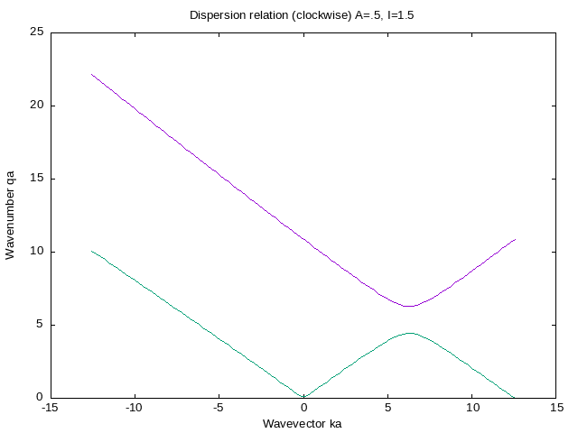
Figure 6: Exact dispersion relation for a left polarized wave propagating with wavevector $\bm{k}$ along the $z$ direction within the same system as in Fig. 2.

From Eq. (38) we may easily find the bandgap edges at $k=G_{0}$,

$$q_{\pm}=\frac{G_{0}}{\sqrt{I\mp A}}.$$ (40)

The reason is that for $\bm{k}=\bm{G}_{0}$, the scattered field has wavevector $\bm{k}-2\bm{G}_{0}=-\bm{G}_{0}$, and, as usual at the border of the Brillouin zone, the field is a stationary wave formed by either an even or an odd combination of the counter propagating components. In the former case, $E_{0-}=E_{s+}$ and the resulting microscopic field is helical, linearly polarized for all $z$ along the local direction of the fibers, so that the response to the field is $I+A$ everywhere, according to Eq. (29). Thus, $k^{2}=G_{0}^{2}=q_{+}^{2}(I+A)$. Similarly, for the odd combination, the field is linearly polarized perpendicular to the direction of the fibers, so the appropriate response is $I-A$ and $G_{0}^{2}=q_{-}^{2}(I-A)$.

Besides the dispersion relation, we may also obtain analytical expressions for the macroscopic permittivity. To that end, consider an external current that propagates with wavevector $\bm{k}$ along the $z$ direction and with right polarization, i.e.

$$\bm{j}_{\text{ex}}=\frac{j_{+}}{\sqrt{2}}\begin{pmatrix}1\\ i\end{pmatrix}e^{ikz}.$$ (41)

This current induces a right polarized wave with wavevector $\bm{k}$ which is scattered by the Bouligand structure into a left circularly polarized wave with wavevector $\bm{k}+2\bm{G}_{0}$. Calling the respective amplitudes $E_{+}$ and $E_{-}$, we rewrite the inhomogeneous wave equation

$$\partial_{z}^{2}\bm{E}+q^{2}\bm{\epsilon}(z)\bm{E}=-\frac{4\pi iq}{c}\bm{j}_{\text{ex}}$$ (42)

as

$$\begin{pmatrix}-k^{2}+q^{2}I&q^{2}A\\ q^{2}A&-(k+2G_{0})^{2}+q^{2}I\end{pmatrix}\begin{pmatrix}E_{+}\\ E_{-}\end{pmatrix}=-\frac{4\pi iq}{c}\begin{pmatrix}j_{+}\\ 0\end{pmatrix}.$$ (43)

Eliminating $E_{-}$ from this system of equation we obtain

$$\left(-k^{2}+q^{2}I+\frac{q^{4}A^{2}}{(k+2G_{0})^{2}-q^{2}I}\right)E_{+}=-\frac{4\pi iq}{c}j_{+}.$$ (44)

Interpreting this equation as a macroscopic inhomogeneous wave equation

$$(-k^{2}+q^{2}\epsilon^{M}_{+})E_{+}=-\frac{4\pi iq}{c}j_{+},$$ (45)

we may identify the macroscopic permittivity for right circular polarization

$$\epsilon^{M}_{+}=I+\frac{q^{2}A^{2}}{(k+2G_{0})^{2}-q^{2}I}.$$ (46)

Similarly, for left circular polarization we obtain

$$\epsilon^{M}_{-}=I+\frac{q^{2}A^{2}}{(k-2G_{0})^{2}-q^{2}I}.$$ (47)

From these, we may readily obtain the permittivity in the cartesian basis,

$$\bm{\epsilon}^{M}=\frac{1}{2}\left(\begin{pmatrix}1\\ i\end{pmatrix}\epsilon^{M}_{+}\begin{pmatrix}1,&i\end{pmatrix}+\begin{pmatrix}1\\ -i\end{pmatrix}\epsilon^{M}_{-}\begin{pmatrix}1,&-i\end{pmatrix}\right).$$ (48)

After some algebra, we obtain analytical expressions for the macroscopic dielectric function of the Bouligand structure,

$$\begin{split}\epsilon^{M}_{xx}&=\epsilon^{M}_{yy}=I+q^{2}A^{2}\frac{k^{2}+4G_{0}^{2}-q^{2}I}{(k^{2}-4G_{0}^{2})^{2}-2q^{2}I(k^{2}+4G_{0}^{2})+q^{4}I^{2}}\\ \epsilon^{M}_{xy}&=-\epsilon^{M}_{yx}=\frac{4ikG_{0}q^{2}A^{2}}{(k^{2}-4G_{0}^{2})^{2}-2q^{2}I(k^{2}+4G_{0}^{2})+q^{4}I^{2}}.\end{split}$$ (49)

We may verify that substitution of this response into the wave equation yields the same dispersion relation as obtained previously, Eq. (39). In Fig. 7 we show the exact non-local macroscopic response corresponding to the same parameters as in Fig. 3.

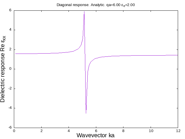
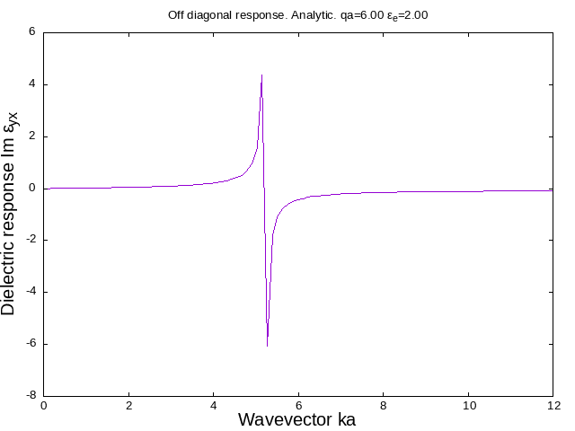
Figure 7: Exact real part of the diagonal diagonal (top) and imaginary part of the off-diagonal (bottom) macroscopic dielectric response, $\epsilon^{M}_{xx}=\epsilon^{M}_{yy}$ and $\epsilon^{M}_{yx}=-\epsilon^{M}_{xy}$ respectively, of the same system as in Fig. 2, with parameters corresponding to Fig. 3.

The figures are almost indistinguishable. Furthermore, from the denominators in Eqs. (49) we can locate the position of the poles,

$$k^{2}_{\infty}=q^{2}I+4G^{2}\pm 4qG\sqrt{I}.$$ (50)

For the parameters used for Fig. 3, there is a pole around $ka=5.22$, as seen in Figs. 3 and 7. There is a second pole around $ka=19.91$ which we have verified is also present in both the numerical as well as the analytic calculation.

V Conclusions

We have been able to extend an efficient homogenization procedure based on Haydock’s recursive algorithm for the calculation of the macroscopic response of a periodic metamaterial made of an arbitrary number of components with an arbitrary composition and an arbitrary geometry. Our extension is based on the observation that using an Euclidean, rather than a Hermitian inner product to define matrix elements of operators, all relevant operators become symmetric, even in the presence of dissipation. However, the inner product couples Bloch waves that propagate in opposite directions, so our formalism requires the simultaneous solution of the field equations for spinor-like fields with two components corresponding to counter-propagating Bloch waves. A previous work [25] followed similar ideas, but was restricted to the non-retarded regime, while the current work is applicable to waves of arbitrary frequency and wavevector. The formalism has been coded into a freely available open source computational package [28]. As a test of our formalism, we have applied it to the calculation of the macroscopic response and the dispersion relation of light within Bouligand-like structures, such as those found in the cuticle of some arthropods. These structures consist of anisotropic layers whose principal axes are continuously rotated as they are stacked on top of each other, yielding chiral helical periodic structures. We found that this structures display optical activity, and that for one helicity they have a photonic gap, which explains the circular polarization upon reflection displayed by the cuticle of some insects. To verify our results we obtained analytical results for these simple systems. Besides having an excelent agreement with the numerical results, encouraging the use with confidence of our Haydock scheme to tackle more complex systems, they allowed us to understand the structure of the macroscopic response, its singularities, the photonic band structure, the polarization of the normal modes, and the position and width of the bandgaps.