Offline and Online Use of Interval and Set-Based Approaches for Control and State Estimation: A Review of Methodological Approaches and Their Application

Abstract.

Control and state estimation procedures need to be robust against imprecisely known parameters, uncertainty in initial conditions, and external disturbances. Interval methods and other set-based techniques form the basis for the implementation of powerful approaches that can be used to identify parameters of dynamic system models in the presence of the aforementioned types of uncertainty. Moreover, they are applicable to a verified feasibility and stability analysis of controllers and state estimators. In addition to these offline approaches for analysis, interval and set-based methods have also been developed in recent years, which allow to solve the associated design tasks and to implement reliable techniques that are applicable online. The latter approaches include set-based model-predictive control, online parameter adaptation techniques for nonlinear variable-structure and backstepping controllers, interval observers, and fault diagnosis techniques. This paper provides an overview of the methodological background and reviews numerous practical applications for which interval and other set-valued approaches have been employed successfully.

1. Introduction

Interval analysis has become an active field of research over the past decades. Its fundamentals can especially be traced back to the works of R.E. Moore and his famous book published in 1966 [57].

In its widest sense, interval analysis provides an approach to perform computations on finitely large sets in such a way that the determined solutions contain all the solutions of the mathematically stated problem with certainty [55, 34]. In such a way, it is not only possible to account for numerical errors due to the limited precision of the numbers representable in floating point arithmetic on a CPU, but also for discretization and method errors. The latter arise inevitably when solving, for example, ordinary differential equations with the help of temporal series expansions truncated after a finite order [60, 61, 38, 53, 12]. In addition to these effects, which are small (at least) for a single evaluation step, but can cause severe damage if neglected, the same techniques also allow for computing with wider sets that result from imperfectly known system parameters and initial conditions in (technical) applications. This lack of knowledge is commonly referred to as epistemic uncertainty [44]. As such, interval analysis provides a mathematically sound way to handle epistemic uncertainty that can furthermore also be traced back to other kinds of a lack of knowledge of the actual system behavior, for example, friction phenomena in rigid body-body dynamics of fluidic applications.

In addition to the application domains mentioned above, further high-level functionalities have been developed on the basis of interval analysis. These contain techniques for solving sets of nonlinear algebraic equations with the help of Newton-type methods [47, 62] or the identification of feasible solution sets that satisfy (nonlinear) constraints in a guaranteed manner [3]. In the latter class of problems, the SIVIA algorithm [34, 91] (set inversion via interval analysis) as well as contractor approaches form the fundamental background, commonly being combined with Newton-type methods. Moreover, extensions exist that allow for handling outliers in a suitable manner by relaxed set intersections [33].

Besides the advantageous features mentioned above that interval techniques always provide guaranteed enclosures of a mathematically formulated problem, they also come with the disadvantage of a certain degree of pessimism. This pessimism is caused by the following two fundamental issues [34, 55, 14]:

• The dependency effect: The difference of two intervals with numerically identical bounds generally does not simplify to the value zero as shown in

  $$\left[{0}\;;\;{1}\right]-\left[{0}\;;\;{1}\right]=\left[{-1}\;;\;{1}\right]\enspace.$$ (1)

  This is due to the fact that the difference in the equation above does not carry any information on whether both arguments are identical quantities or not. Therefore, variables are generally treated as independent in any arithmetic operation according to

  $$\left\{x\circ y|x\in\left[{x}\right]:=\left[{\underline{x}}\;;\;{\overline{x}}\right],y\in\left[{y}\right]:=\left[{\underline{y}}\;;\;{\overline{y}}\right]\right\}~{},\quad\text{where}\quad\circ\in\{+,-,\cdot,/\}\enspace,$$ (2)

  unless simplifications can be carried out on the basis of symbolic formula manipulation, which allows to exploit knowledge that the two arguments $x$ and $y$ represent exactly the same (physical) quantity. Therefore, in classical interval analysis, there do not exist any set-based inversions for the operations of set-based addition and multiplication.

• The wrapping effect: Transformations of sets, for example, rotations and scalings even in linear matrix-vector products as in the recursive evaluation of discrete-time dynamic systems

  $$[{\mathbf{x}}](t_{k+1})=\mathbf{A}\cdot[{\bf{x}}](t_{k})$$ (3)

  with the exemplarily chosen initial conditions and dynamics matrix

  $$\mathbf{x}(t_{0})\in[{\mathbf{x}}](t_{0})=\begin{bmatrix}\left[-1\;;\;1\right]\\ \left[-1\;;\;1\right]\end{bmatrix},~{}\mathbf{A}=\frac{1}{2}\sqrt{2}\begin{bmatrix}1&1\\ -1&1\end{bmatrix}$$ (4)

  may lead to an exponential increase in the volume of the solution enclosures

  $$\mathbf{x}(t_{k})\in 2^{\frac{k}{2}}\cdot\begin{bmatrix}\left[-1\;;\;1\right]\\ \left[-1\;;\;1\right]\end{bmatrix}$$ (5)

  if axis-aligned interval box enclosures were determined in each step (3) despite the fact that the true volume would stay constant in the example above because the matrix $\mathbf{A}$ in (4) represents a volume-preserving rotation of the initial box by $45^{\circ}$ in each step.

In this example, changing the evaluation order according to

$$[{\mathbf{x}}](t_{k+1})=\mathbf{A}^{k+1}\cdot[{\bf{x}}](t_{0})\enspace,$$ (6)

where the integer-order powers of the point-valued matrix $\mathbf{A}$ are firstly determined, allows to solve this problem [46]. However, there is no general solution available, especially in cases where the transformations are nonlinear or the matrices $\mathbf{A}$ may themselves include intervals in each element.

Then, a large variety of other set-representations may turn out to be more efficient, for example, the use of ellipsoids [49, 9] (being mapped exactly to an ellipsoid in point-valued linear transformations), (constrained) zonotopes [32, 82], zonotope bundles [5], or polytopes [76, 85]. In nonlinear settings, the computationally inexpensive thick ellipsoid approach recently published by two of the authors provides the possibility to detect pessimism in the guaranteed outer enclosure by performing a comparison with an inner ellipsoidal enclosure belonging to the solution set with certainty [65, 71]. Moreover, computationally more demanding techniques such as Taylor model arithmetic [12, 11, 13, 31] provide further means to reduce the wrapping effect that is omnipresent in any dynamic system simulation of solution finding to algebraic systems of equations or during the integration of sets of differential equations.

Finally, coordinate transformations, as derived in [39, 40, 56] for systems with either real or complex eigenvalues after their linearization, as well as the exploitation of specific monotonicity properties, allow for reducing both the pessimism discussed above and the computational effort required for its reduction. An example for the exploitation of monotonicity properties is the design of interval observers [64, 20] that allows for computing elementwise lower and upper bounds for the state trajectories according to the following scheme [89].

An autonomous set of ordinary differential equations

$$\dot{\mathbf{x}}(t)={\mathbf{f}}\left({{\mathbf{x}}(t)}\right)~{},~{}~{}\mathbf{x}\in\mathbb{R}^{n}$$ (7)

is cooperative according to [6, 89, 30] if the property

$$x_{i}^{\langle{1}\rangle}\left({t}\right)\geq x_{i}^{\langle{2}\rangle}\left({t}\right)$$ (8)

holds for all elements $i\in\{1,\ldots,n\}$ of the two vectors with $\mathbf{x}^{\langle{1}\rangle}\left({0}\right)$ and $\mathbf{x}^{\langle{2}\rangle}\left({0}\right)$ being the initial conditions which satisfy again the inequalities

$$x_{i}^{\langle{1}\rangle}\left({t_{0}}\right)\geq x_{i}^{\langle{2}\rangle}\left({t_{0}}\right)\quad\text{for all}\quad i\in\{1,\ldots,n\}\enspace.$$ (9)

For continuous-time systems, cooperativity can be checked by the sufficient sign conditions

$$J_{i,j}\left({\mathbf{x}}\right)\geq 0~{},~{}~{}i,j\in\{1,\ldots,n\}~{},~{}~{}i\neq j$$ (10)

for all off-diagonal elements of the Jacobian

$${\mathbf{J}}\left({\mathbf{x}}\right)=\frac{\partial{\mathbf{f}}}{\partial{\mathbf{x}}}\left({{\mathbf{x}}}\right)$$ (11)

of the right-hand side of the state equations evaluated for all reachable states ${\mathbf{x}}={\mathbf{x}}(t)$. Matrices satisfying this non-negativity property for the off-diagonal elements are also denoted as Metzler matrices in the literature [89, 73, 64, 63].

In the case of linear uncertain systems, this cooperativity property simplifies to an elementwise sign condition for the off-diagonal elements of the lower interval bounds of the uncertain dynamics matrix $\mathbf{A}\in\left[{\underline{\mathbf{A}}}\;;\;{\overline{\mathbf{A}}}\right]$ in the dynamic system model

$$\dot{\mathbf{x}}(t)=\mathbf{A}\cdot\mathbf{x}(t)\enspace.$$ (12)

Guaranteed bounds for the state trajectories $\mathbf{x}(t)$ can be obtained in the form $\left[{\mathbf{x}}\right](t)=\left[{\mathbf{v}(t)}\;;\;{\mathbf{w}(t)}\right]$ so that all reachable states are included by an evaluation of the following coupled set of state equations (which are a direct consequence of [58])

$$\begin{split}\dot{v}_{i}(t)&=\inf\left({{[{{A}_{i,i}}]}\cdot v_{i}(t)}\right)+\inf\left({\sum\limits_{j=1\atop j\neq i}^{n}{[{{A}_{i,j}}]}\cdot\left[{z_{j}}\right](t)}\right)\\ \dot{w}_{i}(t)&=\sup\left({{[{{A}_{i,i}}]}\cdot w_{i}(t)}\right)+\sup\left({\sum\limits_{j=1\atop j\neq i}^{n}{[{{A}_{i,j}}]}\cdot\left[{z_{j}}\right](t)}\right)\end{split}$$ (13)

with the resulting state bounds

$$\left[{{z}_{i}}\right](t)=\left[{{v}_{i}(t)}\;;\;{{w}_{i}(t)}\right]\enspace.$$ (14)

In the equations above, the operators $\inf\left({\cdot}\right)$ and $\sup\left({\cdot}\right)$ denote the lower and upper interval bounds of the corresponding arguments.

Note that couplings between the vectors $\mathbf{v}(t)$ and $\mathbf{w}(t)$ can be ignored in (13) if the system is positive, i.e., $v_{i}(t)\geq 0$ holds for all $t\geq 0$, see for example [64, 20]. There, this property is exploited for the design of a Luenberger-type interval observer, which allows for guaranteed state estimation in the case of bounded measurement uncertainty.

Moreover, recent developments of the so-called mixed monotonicity approach and remainder form decompositions [43, 42] can be exploited as a relaxation of the aforementioned evaluation technique based on cooperativity. In this case, a cooperative subsystem is extracted from the dynamic system model, while the non-cooperative part is shifted in to an additive bounded error term. In such a way, the possibility for extracting bounding systems is preserved and the need for computing with general sets is still avoided.

For practical implementation of set-valued calculus, numerous software libraries exist. The following short list is given without any claim for completeness: IntLab [86] for Matlab and Octave, the Octave interval package [28], Versoft [83], Juliaintervals [87], C-XSC [45], DynIbex [1], the CORA library [4], and codac [84].

This paper is structured as follows. Sec. 2 gives an overview of the fundamentals of identifying parameters for dynamic systems with the help of interval and other set-based approaches. These identification results are the basis for the variable-structure control approaches reviewed in Sec. 3 as well as for the guaranteed model-predictive control approaches in Sec. 4. Thereafter, we present approaches for set-based state estimation in Sec. 5, applicable to the identification of the open-circuit voltage characteristic of Lithium-ion batteries, and an ellipsoidal technique in Sec. 6 that allows for treating set-valued and stochastic uncertainty and disturbances in a unified manner when solving state estimation tasks. Finally, conclusions and a brief outlook on future work are given in Sec. 7.

2. System Modeling and Verified Parameter Identification

The estimation of the parameters of both finite-dimensional sets of discrete-time difference equations as well as continuous-time ordinary differential equations is crucial for the design and implementation of all model-based control and state estimation procedures. Identification experiments are typically performed (for asymptotically stable systems) with predefined, time-dependent actuation signals so that measurements of selected outputs can be gathered at certain discrete points of time $t_{k}$, $k\in\mathbb{N}_{0}$. Here, $t_{0}=0$ is assumed without loss of generality. Due to the collection of measurements at discrete points of time, it is necessary that parameter identification routines allow for a propagation of state information between two subsequent measurement instants $t_{k-1}$ and $t_{k}$, $k\geq 1$. The following description of the set-based parameter identification approach is based on the more detailed discussions that can be found in [74].

2.1. Predictor–Corrector Framework for the Verified Identification of Parameters of Dynamic Systems

As summarized in Fig. 1, a first class of verified parameter identification routines is characterized by an observer-based structure. This structure is closely linked to the evaluation steps that are performed in classical state estimators such as Luenberger-type observers or (Extended) Kalman Filters [37, 35]. Hence, prediction and correction steps are separated from each other and evaluated in an alternating manner.

In this framework, the detection of feasible parameter domains is performed by means of the following three-stage procedure [69, 19]:

1. A verified evaluation of the set of state equations is performed between two subsequent measurement points. In the case of discrete-time state equations, the corresponding expressions are evaluated with the help of interval arithmetic (or one of the alternative set-valued approaches mentioned in the introduction of this article), while verified solvers for initial value problems for ordinary differential equations [2, 52, 38, 61, 7, 59, 1, 60, 48] are required if continuous-time processes are taken into consideration. In any case, problem-specific approaches for the reduction of overestimation [75] — such as interval subdivision, preconditioning of state equations, symbolic simplifications, or enclosures allowing to trace the shape of the reachable state domains in a tight manner — shall be employed to minimize the pessimism in the computed state and output boundaries that is caused by both the dependency and wrapping effects [34, 53].

2. Information resulting from the prediction of state intervals up to the point at which new measurements are available are combined with information obtained from sensors. The applicable techniques are:

   • A direct intersection of the enclosures of predicted state variables with directly measured state intervals (in terms of an additive superposition of a point-valued measurement with the respective tolerance interval);

   • The use of contractors and set inversion approaches to determine an inverse mapping from the measured outputs to the internal system states and parameters [32]. Example are forward–backward contractors [34] initialized with the predicted state intervals that are intersected with the associated measurement outputs or interval Newton techniques in the case of nonlinear output equations or for output equations involving more than one state variable.

3. Parameter subdomains are eliminated either by the contractors for which details are presented in the following section or after a subdivision of parameter intervals with associated multiple evaluations of the state equations. In the latter case, a parameter subinterval is guaranteed to be inconsistent with the information provided by the specified system model and the available measurements if the result of the state prediction substituted into the measurement model and the interval-valued measured data do not overlap. For a visualization of this exclusion text, see Fig. 2, where a branch-and-bound procedure on the basis of multiple simulations of the state equations over the complete horizon of gathered measured data is depicted. The corresponding consistency tests correspond to those also used in the following subsection.

Figure 1. Predictor–corrector scheme for combined state estimation and parameter identification [74].

2.2. Simulation-Based Parameter Identification Procedures

Simulation-based parameter identification procedures, making use of multiple evaluations of the set of state equations for subintervals of the complete initial domain of possible system parameters, are a second option for parameter identification.

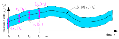
(a) Measurement information of the system output $y_{\mathrm{m}}(t)$, sampled at the equidistant instants $t_{0},t_{1},t_{2},\ldots$.

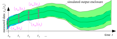
(b) Output trajectory including interval uncertainty for a possibly feasible (undecided) system parameterization (Case 1).

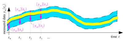
(c) Output trajectory including interval uncertainty for a guaranteed feasible system parameterization (Case 2).

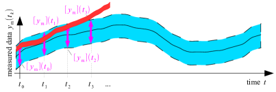
(d) Output trajectory including interval uncertainty for a guaranteed infeasible system parameterization (Case 3).

Figure 2. Simulation-based distinction between possibly feasible, guaranteed feasible, and infeasible system parameterizations [19, 74].

The underlying branch-and-bound procedure relies on the following assumptions:

• measured data are available at discrete points of time,

• worst-case bounds for measurement tolerances are known a-priori (modeling of the sensor uncertainty),

• the model structure to be parameterized is assumed to be structurally correct,

• outer enclosures for the domains of possibly uncertain initial states are given, and

• interval bounds on the uncertain parameters are known in terms of conservative overapproximations.

To exclude parts of the domains of uncertain initial states and parts of the a-priori given parameter intervals, a subdivision procedure of the respective domains is executed [15]. To detect intervals for the parameterization of the system model which are guaranteed to be inconsistent, directly measured and simulated state intervals are intersected at identical points of time. If state variables are not directly measured, the contractor procedures mentioned in the previous subsection are equally applicable here. Parameter interval subdivisions are performed according to the following distinction of cases, where the directions in which the determined parameter intervals are subdivided with the help of a sensitivity analysis [19]. For accelerations by both additional (physics-inspired) contractors and GPU-based parallelizations, the readers are referred to [74, 8]:

Case 1:

Parameter subintervals are yet undecided if their corresponding predicted output intervals overlap at least partially for all available sensors at each point of time at which measurements are available and are never outside the range of measured data.

Case 2:

A parameter subinterval is guaranteed to be consistent if the corresponding output intervals are true subintervals of the interval-valued measured data for each of the available sensors at each point of time. This subinterval is no longer investigated but stored in a list of guaranteed admissible boxes.

Case 3:

A parameter subinterval is guaranteed to be inconsistent if the corresponding output interval lies outside the range of the interval-valued measured data. This has to hold true for at least one of the available sensors and for at least one point in time. The resulting parameter subinterval is excluded from further evaluations and the underlying simulation can be aborted as soon as the inconsistency is detected.

3. Interval-Based Variable-Structure Control Implementation

As mentioned in the previous section, the verified parameter identification is the prerequisite for the implementation of guaranteed stabilizing control procedures. These include linear matrix inequality methods for systems with polytopic and norm-bounded parameter uncertainty [10, 73], interval-based gain scheduling techniques [41], and variable structure as well as backstepping-type controllers [88, 77, 80, 78] without and with hard state constraints.

In this section, we review a robust control procedure that extends the sliding mode design methodology by means of the online use of interval analysis to prevent the violation of state constraints with certainty [88, 77, 79]. For a similar approach, applicable to the backstepping design methodology, the reader is referred to [72].

3.1. Fundamental Sliding Mode Control Laws

Both the treatment of strict inequality constraints and bounded interval uncertainty can be combined with first- and second-order sliding mode techniques [21, 26].

3.1.1. First-Order Sliding Mode Control

For a summary of the fundamental sliding mode control design of single-input single-output systems, consider the $n$-th order set of ordinary differential equations

$$\begin{split}\dot{\mathbf{x}}(t)&\!=\!\begin{bmatrix}\dot{x}_{1}(t)&\ldots&\dot{x}_{n-1}(t)&\dot{x}_{n}(t)\end{bmatrix}^{T}\\ &\!=\!\begin{bmatrix}{x}_{2}(t)&\ldots&{x}_{n}(t)&a\left({{\mathbf{x}}(t),{\mathbf{p}}}\right)+b\left({{\mathbf{x}}(t),{\mathbf{p}}}\right)\!\cdot\!v(t)\end{bmatrix}^{T}\end{split}$$ (15)

in nonlinear controller canonical form with the state vector ${\mathbf{x}}(t)\in\mathbb{R}^{n}$ and the control input ($b\left({{\mathbf{x}}(t),{\mathbf{p}}}\right)\neq 0$)

$$v(t)=\frac{-a\left({{\mathbf{x}}(t),{\mathbf{p}}}\right)+u(t)}{b\left({{\mathbf{x}}(t),{\mathbf{p}}}\right)}\in\mathbb{R}\enspace.$$ (16)

For this system model, the output variable is given by

$$y(t)=x_{1}(t)\enspace.$$ (17)

Due to the assumed structure of the system (15), the output variable (17) has the relative degree $n$ [54], corresponding to the property that the $n$-th time derivative $x_{1}^{(n)}(t)$ of the system output is the lowest-order derivative explicitly depending on either of the control inputs $v(t)$ and $u(t)$. Therefore, the output $y(t)$ corresponds to a (trivial) flat system output [23] and an exact tracking of a sufficiently smooth desired trajectory $x_{1,\mathrm{d}}(t)$ can be achieved in the case of exactly known parameters.

On the basis of this desired trajectory, the corresponding tracking error ($r=0$) and its $r$-th time derivative are given by

$$\tilde{\xi}_{1}^{(r)}=x_{1}^{(r)}-x_{1,\mathrm{d}}^{(r)}~{},~{}~{}r\in\{0,1,\ldots,n\}\enspace,$$ (18)

with the sliding surface

$$s:=s(t)=\sum\limits_{r=0}^{n-1}\alpha_{r}\tilde{\xi}_{1}^{(r)}$$ (19)

in which the highest-order coefficient is normalized according to $\alpha_{n-1}=1$. To guarantee asymptotic stability for states exactly located on this sliding surface, the parameters $\alpha_{r}$ have to fulfill the necessary and sufficient stability conditions for a Hurwitz polynomial of the order $n-1$.

A classical first-order sliding mode control can be derived with the help of the quadratic radially unbounded candidate for a Lyapunov function

$$V^{\langle{\mathrm{I}}\rangle}=\frac{1}{2}s^{2}>0\quad\text{for}\quad s\neq 0\enspace.$$ (20)

For $s\neq 0$, (global) asymptotic stability of the dynamic system corresponds to the (global) negative definiteness of the corresponding time derivative

$$\dot{V}^{\langle{\mathrm{I}}\rangle}=s\cdot\dot{s}=\left({\sum\limits_{r=0}^{n-1}\alpha_{r}\tilde{\xi}_{1}^{(r)}}\right)\cdot\left({\sum\limits_{r=0}^{n-1}\alpha_{r}\tilde{\xi}_{1}^{(r+1)}}\right)<0\enspace.$$ (21)

Following the derivation of the variable-structure control law according to [80, 78], the right-hand side of the inequality (21) is replaced by the more conservative formulation

$$\left({\sum\limits_{r=0}^{n-1}\alpha_{r}\tilde{\xi}_{1}^{(r)}}\right)\cdot\left({\sum\limits_{r=0}^{n-1}\alpha_{r}\tilde{\xi}_{1}^{(r+1)}}\right)<-\eta\cdot\left|s\right|=-\eta\cdot\left({\sum\limits_{r=0}^{n-1}\alpha_{r}\tilde{\xi}_{1}^{(r)}}\right)\cdot\mathrm{sign}\left({s}\right)$$ (22)

which guarantees global asymptotic stability for $\eta>0$. Here, the actual choice of $\eta$ significantly influences the dynamics and the maximum absolute values of the control signal in the reaching phase characterized by $s\neq 0$. As soon as $s=0$ has been reached after a finite time duration, the control amplitudes depend (in the unperturbed case) on the actual choice of the reference trajectory $x_{1,\mathrm{d}}$ and on the coefficients $\alpha_{r}$.

These latter values also have a major influence on the control amplitudes if non-modeled errors and disturbances act on the system dynamics and if the error signals $\tilde{\xi}_{1}^{(r)}$ are corrupted by non-negligible measurement noise or state reconstruction errors, preventing the perfect tracking of the desired trajectory $x_{1,\mathrm{d}}(t)$ and making it impossible that $s\equiv 0$ holds perfectly after the end of the reaching phase.

The derivation of the control law is completed by enforcing that the second factor in (22) becomes proportional to the sign of the actual value of $s$ according to

$$\sum\limits_{r=0}^{n-2}\alpha_{r}\tilde{\xi}_{1}^{(r+1)}+u-x_{1,\mathrm{d}}^{(n)}+\eta\cdot\mathrm{sign}\left({s}\right)=-\beta\cdot\mathrm{sign}\left({s}\right)\quad\text{with}\quad\beta>0\enspace.$$ (23)

Using $\tilde{\eta}:=\eta+\beta>0$, the control law results in

$$u(t)=u^{\langle{\mathrm{I}}\rangle}=x_{1,\mathrm{d}}^{(n)}-\sum\limits_{r=0}^{n-2}\alpha_{r}\tilde{\xi}_{1}^{(r+1)}-\tilde{\eta}\cdot\mathrm{sign}\left({s}\right)\enspace.$$ (24)

3.1.2. Second-Order Sliding Mode Control

For a second-order sliding mode, both $s=0$ and $\dot{s}=0$ have to be ensured by the feedback controller [21, 26]. This can be achieved by adding a first-order lag dynamics on the left-hand side of

$$\gamma_{1}\dot{s}+\gamma_{0}s=\sum\limits_{r=-1}^{n-1}\alpha_{r}\tilde{\xi}_{1}^{(r)}\quad\text{with}\quad\tilde{\xi}_{1}^{(-1)}(t):=\int_{0}^{t}\tilde{\xi}_{1}(\tau)\mathrm{d}\tau\,.$$ (25)

For the sake of asymptotic stability, the coefficients $\gamma_{0}$ and $\gamma_{1}$ need to be strictly positive. For $\alpha_{-1}=0$, this sliding surface has a proportional and differentiating characteristic, while $\alpha_{-1}\neq 0$ means that the integral $\tilde{\xi}_{1}^{(-1)}$ of the output error is additionally fed back in the definition of the sliding variable $s$.

To ensure both $s=0$ and $\dot{s}=0$ for the closed-loop control system, the Lyapunov function candidate, which was previously chosen as a function solely depending on the value of $s$, is redefined in the form

$$V^{\langle{\mathrm{II}}\rangle}=\frac{1}{2}\cdot\left({s^{2}+\lambda\dot{s}^{2}}\right)\quad\text{with the scaling factor}\quad\lambda>0\enspace.$$ (26)

The computation of the time derivative of (26) results in

$$\dot{V}^{\langle{\mathrm{II}}\rangle}=s\cdot\dot{s}+\dot{s}\cdot\left({-\frac{\lambda\gamma_{0}}{\gamma_{1}}\dot{s}+\frac{\lambda}{\gamma_{1}}\sum\limits_{r=0}^{n}\alpha_{r-1}\tilde{\xi}_{1}^{(r)}}\right)<0\enspace,$$ (27)

where $\lambda=\gamma_{1}>0$ is used without loss of generality [77]. Also according to [77], the stabilization of the closed-loop system towards $s=0$ can be achieved by setting

$$\dot{V}^{\langle{\mathrm{II}}\rangle}<-\eta_{1}\cdot\left|\dot{s}\right|-\eta_{2}\cdot\left|{s}\right|\cdot\left|\dot{s}\right|=-\dot{s}\cdot\mathrm{sign}\left({\dot{s}}\right)\cdot\left({\eta_{1}+\eta_{2}\cdot\left|{s}\right|}\right).$$ (28)

This finally leads to the nonlinear feedback controller [21, generalized form of Eqs. (22), (23)]

$$u=u^{\langle{\mathrm{II}}\rangle}=x_{1,\mathrm{d}}^{(n)}+\frac{1}{\alpha_{n-1}}\cdot\Biggl{(}\gamma_{0}\dot{s}-s-\sum\limits_{r=0}^{n-1}\alpha_{r-1}\tilde{\xi}_{1}^{(r)}-\mathrm{sign}\left({\dot{s}}\right)\cdot\left({\tilde{\eta}_{1}+\tilde{\eta}_{2}\cdot\left|{s}\right|}\right)\Biggr{)}$$ (29)

with $\tilde{\eta}_{i}\geq\eta_{i}>0$ for both $i\in\{1,2\}$.

3.2. Extension by One- and Two-Sided Barrier Functions

Both control laws $u^{\langle{\mathrm{I}}\rangle}$ and $u^{\langle{\mathrm{II}}\rangle}$ can be extended by one- and two-sided barrier functions  [90].

3.2.1. One-Sided State Constraints

For the case of a one-sided barrier, it is necessary that the (time-varying) state (respectively output) constraint

$$x_{1}<\bar{x}_{1,\mathrm{max}}:=x_{1,\mathrm{d}}+\Delta{x}_{1,\mathrm{max}}\quad\text{with}\quad\Delta{x}_{1,\mathrm{max}}>0$$ (30)

is not violated for any point of time $t>0$ if the initial conditions for the state vector ${\mathbf{x}}(t)$ at $t=0$ are also compatible with this constraint. Moreover, it is necessary that the sliding surface $s=0$ (equivalent to $x_{1}=x_{1,\mathrm{d}}$) lies within the admissible operating range defined in (30).

Then, the extended Lyapunov function ansatz

$$\begin{split}{V}^{\langle{j,\mathrm{A}}\rangle}&=V^{\langle{j}\rangle}+V^{\langle{\mathrm{A}}\rangle}>0\quad\text{for}\quad s\neq 0\quad\text{with}\end{split}$$ (31)

$$V^{\langle{\mathrm{A}}\rangle}=\rho_{\mathrm{V}}\cdot\ln\left({\tfrac{\sigma_{\mathrm{V}}\cdot\bar{x}_{1,\mathrm{max}}}{\bar{x}_{1,\mathrm{max}}-x_{1}}}\right)~{}\text{and}~{}x_{1}<\bar{x}_{1,\mathrm{max}}$$ (32)

is introduced for both alternatives $j\in\{\mathrm{I},\mathrm{II}\}$. In (32), $\rho_{\mathrm{V}}>0$ is selected so that the singularity ${\bar{x}_{1,\mathrm{max}}-x_{1}}=0$ represents a repelling potential and that control constraints are not violated for usual operating conditions. Then, the term $V^{\langle{j}\rangle}$ has dominating influence in the neighborhood of $s=0$, while $\sigma_{\mathrm{V}}>0$ can be used to adapt the steepness of the barrier function near its singularity.

In the case of the first-order sliding mode, the time derivative of (31) can be computed as

$$\dot{V}^{\langle{j,\mathrm{A}}\rangle}=\dot{V}^{\langle{j}\rangle}+\dot{V}^{\langle{\mathrm{A}}\rangle}<0\quad\text{with}\quad\dot{V}^{\langle{\mathrm{A}}\rangle}=\tfrac{\rho_{\mathrm{V}}}{\bar{x}_{1,\mathrm{max}}}\cdot\left({\tfrac{-x_{1}\cdot\dot{\bar{x}}_{1,\mathrm{max}}+\dot{x}_{1}\cdot\bar{x}_{1,\mathrm{max}}}{\bar{x}_{1,\mathrm{max}}-x_{1}}}\right)\enspace,$$ (33)

where $\dot{V}^{\langle{\mathrm{A}}\rangle}$ does not explicitly depend on the system input $u$.

In analogy to the fundamental first-order sliding mode control law $u^{\langle{\mathrm{I}}\rangle}(t)$ derived from (23), the inequality

$$s\cdot\underbrace{\left({\sum\limits_{r=0}^{n-2}\alpha_{r}\tilde{\xi}_{1}^{(r+1)}+u-x_{1,\mathrm{d}}^{(n)}+\eta\cdot\mathrm{sign}\left({s}\right)+\frac{1}{s}\cdot\dot{V}^{\langle{\mathrm{A}}\rangle}}\right)}_{-\beta\cdot\mathrm{sign}\left({s}\right)}<0$$ (34)

is obtained. Following the same steps as in the derivation of $u^{\langle{\mathrm{I}}\rangle}(t)$ yields the control law

$$u={u}^{\langle{\mathrm{I},\mathrm{A}}\rangle}=u^{\langle{\mathrm{I}}\rangle}-\tfrac{s}{s^{2}+\tilde{\epsilon}}\cdot\dot{V}^{\langle{\mathrm{A}}\rangle}\enspace,$$ (35)

in which $\frac{1}{s}$ in (34) has been approximated by $\frac{s}{s^{2}+\tilde{\epsilon}}$ with the small constant $\tilde{\epsilon}>0$ to ensure regularity of the control law ${u}^{\langle{\mathrm{I},\mathrm{A}}\rangle}(t)$ on the sliding surface $s=0$. Moreover, this modification guarantees that the barrier function becomes inactive as soon as the control goal has been reached.

In analogy to (35), the second-order sliding mode control (29) can be extended by the barrier function (32). Following the same steps as in Eqs. (33)–(35) leads to

$$u={u}^{\langle{\mathrm{II},\mathrm{A}}\rangle}=u^{\langle{\mathrm{II}}\rangle}-\tfrac{1}{\alpha_{n-1}}\cdot\tfrac{\dot{s}}{\dot{s}^{2}+\tilde{\epsilon}}\cdot\dot{V}^{\langle{\mathrm{A}}\rangle}\enspace.$$ (36)

3.2.2. Two-Sided State Constraints

For the case of two-sided state constraints, the Lyapunov functions $V^{\langle{j}\rangle}$, $j\in\{\mathrm{I},\mathrm{II}\}$, are extended according to

$${V}^{\langle{j,\mathrm{B}}\rangle}=V^{\langle{j}\rangle}+V^{\langle{\mathrm{B}}\rangle}>0\quad\text{for}\quad s\neq 0\enspace,$$ (37)

where the additive term $V^{\langle{\mathrm{B}}\rangle}$ is chosen in this paper so that state deviations $\left|x_{1}-x_{1,\mathrm{d}}\right|\geq\bar{\chi}$ are prevented. For the alternative option $\left|s\right|\geq\bar{\chi}$, the reader is referred to [77]. Symmetric barriers can be enforced by specifying a barrier function in the form

$$V^{\langle{\mathrm{B}}\rangle}=\rho_{\mathrm{V}}\cdot\ln\left({\tfrac{\bar{\chi}^{2l}}{\bar{\chi}^{2l}-\left({x_{1}-x_{1,\mathrm{d}}}\right)^{2l}}}\right)\quad\text{with}\quad l\in\mathbb{N}\enspace.$$ (38)

Large values for $l$ typically lead to the fact that resulting state trajectories come closer to the edges of the admissible operating range. As before, the time derivative of the additive term (38) is computed, which yields

$$\dot{V}^{\langle{\mathrm{B}}\rangle}=\rho_{\mathrm{V}}\cdot\tfrac{{2l}\cdot\left({x_{1}-x_{1,\mathrm{d}}}\right)^{2l-1}\cdot\left({\dot{x}_{1}-\dot{x}_{1,\mathrm{d}}}\right)}{\bar{\chi}^{2l}-\left({x_{1}-x_{1,\mathrm{d}}}\right)^{2l}}\enspace.$$ (39)

In full analogy to Eqs. (33)–(36), the requirement $\dot{V}^{\langle{j,\mathrm{B}}\rangle}<0$ for $s\neq 0$ (and $\dot{s}\neq 0$, resp.) leads to the extension

$${u}^{\langle{\mathrm{I},\mathrm{B}}\rangle}=u^{\langle{\mathrm{I}}\rangle}-s^{-1}\cdot\dot{V}^{\langle{\mathrm{B}}\rangle}$$ (40)

of the first-order sliding mode controller and to

$${u}^{\langle{\mathrm{II},\mathrm{B}}\rangle}=u^{\langle{\mathrm{II}}\rangle}-\left({\alpha_{n-1}\cdot\dot{s}}\right)^{-1}\cdot\dot{V}^{\langle{\mathrm{B}}\rangle}$$ (41)

for the second-order case, where the same regularization strategies for the rational terms $\frac{1}{s}$ and $\frac{1}{\dot{s}}$ become necessary as before. The term $\dot{s}$ (if required) is typically estimated by a low-pass filtered differentiation or by means of an observer.

3.3. Interval Extensions to Handle Bounded Parameter Uncertainty and State Estimation Errors

To guarantee asymptotic stability despite bounded uncertainty in both the measured (resp., estimated) states $\mathbf{x}$ and system parameters ${\mathbf{p}}$ included in the control law, interval techniques can be applied at run-time during the execution of the previously derived control laws if they are extended according to [78, 77]. ${\mathbf{x}}\in\left[{{\mathbf{x}}}\right]=\left[{\underline{\mathbf{x}}}\;;\;{\overline{\mathbf{x}}}\right]$ of the measured or estimated state vector. In addition, it is assumed that the system model is given as an $n$-th order set of ODEs (15) in nonlinear controller canonical form. If this is not the case, extended control approaches according to [88] are applicable.

For the sake of controllability (and, hence, also for the existence of the following interval-based variable-structure controllers), it has to be guaranteed that

$$0\not\in b\left({\left[{\mathbf{x}}\right],\left[{\mathbf{p}}\right]}\right)$$ (42)

holds for all ${\mathbf{x}}\in\left[{{\mathbf{x}}}\right]$ and ${\mathbf{p}}\in\left[{{\mathbf{p}}}\right]$, describing, respectively, the reachable domain in the state-space and the guaranteed enclosure of all uncertain parameters. To handle the set-valued state and parameter uncertainty, the output tracking error and its $r$-th derivative are enclosed by the intervals

$$\tilde{\xi}_{1}^{(r)}\in\left[{\tilde{\xi}_{1}^{(r)}}\right]=\left[{x_{1}^{(r)}}\right]-x_{1,\mathrm{d}}^{(r)}$$ (43)

for each $r\in\{0,1,\ldots,n\}$. These tracking error intervals can be used to generalize the first-order variable-structure controller (without and with state constraints) according to

$$\left[{v^{\langle{\mathrm{I}}\rangle}}\right]=\tfrac{-a\left({\left[{{\mathbf{x}}}\right],\left[{{\mathbf{p}}}\right]}\right)+x_{1,\mathrm{d}}^{(n)}-\sum\limits_{r=0}^{n-2}\alpha_{r}\cdot\left[{\tilde{\xi}_{1}^{(r+1)}}\right]-\tilde{\eta}\cdot\mathrm{sign}\left({\left[{s}\right]}\right)}{b\left({\left[{\mathbf{x}}\right],\left[{\mathbf{p}}\right]}\right)}\enspace,$$ (44)

$$\left[{{v}^{\langle{\mathrm{I},\mathrm{A}}\rangle}}\right]=\left[{v^{\langle{\mathrm{I}}\rangle}}\right]-\tfrac{1}{b\left({\left[{\mathbf{x}}\right],\left[{\mathbf{p}}\right]}\right)}\cdot\tfrac{\left[{s}\right]}{\left[{s}\right]^{2}+\tilde{\epsilon}}\cdot\left[{\dot{V}^{\langle{\mathrm{A}}\rangle}}\right]\enspace,$$ (45)

and

$$\left[{{v}^{\langle{\mathrm{I},\mathrm{B}}\rangle}}\right]=\left[{v^{\langle{\mathrm{I}}\rangle}}\right]-\tfrac{1}{b\left({\left[{\mathbf{x}}\right],\left[{\mathbf{p}}\right]}\right)}\cdot\tfrac{\left[{s}\right]}{\left[{s}\right]^{2}+\tilde{\epsilon}}\cdot\left[{\dot{V}^{\langle{\mathrm{B}}\rangle}}\right]\enspace.$$ (46)

Similarly, interval-based generalizations can be defined for all before-mentioned second-order formulations. For a detailed discussion of restrictions in the case that accounts for integrator extensions in the definition of the sliding surface $s=0$, the reader is referred to [77].

In all expressions above, $a\left({\left[{\mathbf{x}}\right],\left[{\mathbf{p}}\right]}\right)$, ${b\left({\left[{\mathbf{x}}\right],\left[{\mathbf{p}}\right]}\right)}$, $\left[{\dot{V}^{\langle{\mathrm{A}}\rangle}}\right]$, and $\left[{s}\right]$ denote the interval-dependent evaluations of the corresponding entries of the state equations, the time derivatives of the barrier function, and the sliding surface, respectively. For the actual control implementation, all interval expressions are evaluated by means of a suitable interval library.

In previous work such as [72, 79, 78, 77], where this approach was applied successfully to the control of the thermal behavior of high-temperature solid oxide fuel cells as well as for the control of inverted pendulum systems, the C++ toolbox C-XSC [45] was used. Required derivatives, necessary to transform general nonlinear state equations into the system representation assumed in this section, can easily be obtained with the help of algorithmic differentiation. The template-based library FADBAD++ has shown its efficiency for this purpose, because it cannot only be applied to expressions involving classical point-valued data types but also interval variables.

It has to be pointed out that the actual implementation of the control laws (44)–(46) is performed in such a way that a point-valued control signal $v$ is chosen from the computed intervals so that it guarantees asymptotic stability regardless of the sign of ${b}({\mathbf{x}},{\mathbf{p}})$. According to [77], this is done by testing the negative definiteness of the Lyapunov function candidate for the infima and suprema $\underline{v}:=\mathrm{inf}\{\left[{v}\right]\}$ and $\overline{v}:=\mathrm{sup}\{\left[{v}\right]\}$. To account for roundoff and representation errors, these values are inflated by a small constant $\epsilon>0$ to obtain the final set of candidates $\mathcal{V}:=\left\{\underline{v}-\epsilon,\underline{v}+\epsilon,\overline{v}-\epsilon,\overline{v}+\epsilon\right\}$, from which the signal with minimum absolute value is chosen that ensures $\dot{V}<0$ (or more generally $\dot{V}^{\langle{j,\mathrm{A}}\rangle}<0$, $\dot{V}^{\langle{j,\mathrm{B}}\rangle}<0$, $j\in\{\mathrm{I},\mathrm{II}\}$) despite the considered interval uncertainty.

4. Guaranteed Model Predictive Control

Predictive control techniques are powerful approaches for controlling uncertain systems, where the corresponding dynamics are formulated initial value problems for finite-dimensional sets of nonlinear ordinary differential equations. Besides stabilizing the dynamics towards a desired reference trajectory, it is possible to formulate the involved optimization problem in such a way that constraints for the admissible state trajectories and system inputs are handled. Classical approaches for nonlinear model predictive control commonly do not account for interval bounds in initial states and system parameters. This issue is resolved in this section, by presenting a control procedure for interval-valued initial value problems in the form [25]

$$\left\{\begin{array}[]{l}\dot{\mathbf{x}}(t)=\mathbf{f}(t,\mathbf{x}(t),\mathbf{u},\mathbf{p})\\ \mathbf{x}_{0}\in\left[\mathbf{{x}}_{0}\right]\subseteq{\mathbb{IR}}^{n}\\ \mathbf{u}\in\left[\mathbf{{u}}\right]\subseteq{\mathbb{IR}^{m}}\\ \mathbf{p}\in\left[\mathbf{{p}}\right]\subseteq{\mathbb{IR}^{p}},\end{array}\right.$$ (51)

where the state vector is denoted by $\mathbf{x}(t)$, the vector of dynamic parameters by $\mathbf{p}$, and the control vector by $\mathbf{u}$. The sets $\left[\mathbf{{x}}_{0}\right]=\begin{bmatrix}\left[{{x}}_{10}\right]&\ldots&\left[{{x}}_{n0}\right]\end{bmatrix}^{T}$, $\left[\mathbf{{u}}\right]=\begin{bmatrix}\left[{{u}}_{1}\right]&\ldots&\left[{{u}}_{m}\right]\end{bmatrix}^{T}$, and $\left[\mathbf{{p}}\right]=\begin{bmatrix}\left[{{p}}_{1}\right]&\ldots&\left[{{p}}_{\mathrm{p}}\right]\end{bmatrix}^{T}$, expressed as interval boxes, are respectively the initial condition of the state vector, the interval-bounded input, and the set of feasible dynamic parameters. We assume that this interval-based initial value problem has a unique solution $\mathbf{x}(t)(t,\mathbf{x}_{0},\mathbf{u},\mathbf{p})$ at $t>0$ since $\mathbf{f}:\mathbb{R}\times\mathbb{R}^{n}\times\mathbb{R}^{m}\times\mathbb{R}^{p}\rightarrow\mathbb{R}^{n}$ is supposed to be continuous in $t$ and Lipschitz in $\mathbf{x}(t)$. For the use of the proposed solution algorithm, we further require that $\mathbf{f}$ is sufficiently smooth, i.e., of class $C^{k}$. For an approach applicable to linear time-invariant and linear parameter-varying systems, which is similar to the one described subsequently, the reader is referred to [18, 16, 17].

4.1. Interval-Based Nonlinear Model Predictive Control

The interval-based nonlinear model predictive control approach presented in [25, 24] is a generalization of the optimization approach in [70] and is based on the computation of interval bounds for the control sequence over a receding horizon which takes into account bounded uncertainties in the parameters of the dynamic system model and in the measured data.

The control intervals are calculated such that the convergence to the set-point interval is ensured (i.e., $\textbf{x}(t_{j})\to[\textbf{x}_{\mathrm{r}}],~{}~{}\forall j$, and all the state and input constraints are satisfied (i.e., $\textbf{x}(t_{i})\in[\textbf{x}(t_{i})]$ and $\textbf{u}(t_{j})\in[\textbf{u}(t_{j})],~{}~{}\forall i,j$). The corresponding interval algorithm encompasses two stages [24], namely,

• Filtering and branching: This first step provides a sequence of guaranteed input interval boxes at each time-step $t_{k}$ over the prediction horizon $N_{\mathrm{p}}$, denoted as $[\mathbf{U}(t_{k})]=[\mathbf{{u}}(t_{k})]\times[\mathbf{{u}}{(t_{k+1})}]\times\ldots\times[\mathbf{{u}}(t_{k+N_{\mathrm{p}}-1})]$. Branching and filtering procedures allow the computation of safe input intervals along the receding time horizon that satisfy the state constraints (i.e., $\forall j,\left[\mathbf{{x}}(t_{j})\right]\subseteq[\mathbf{x}_{\min}(t_{j}),\mathbf{x}_{\max}(t_{j})]$, where $\mathbf{x}_{\min}(t_{j})$ and $\mathbf{x}_{\max}(t_{j})$ are the bounds for the admissible domain for each state variable) and ensure convergence to the reference interval (i.e., $[\mathbf{x}_{k}]\rightarrow[\mathbf{x}_{\mathrm{r}}]$).

• Interval optimization: Since safe inputs are computed over a finite time horizon, the optimization algorithm is launched to compute the optimal inputs $[\mathbf{U}(t_{k})]^{\star}$ by minimizing as much as possible a newly formulated interval objective function to reduce both the norm of the input intervals and the error between the predicted as well as the reference outputs.

4.2. Formulation and Minimization of Interval Cost Functions

For the feasible intervals of input values that satisfy the constraints on the state trajectories and system inputs, an optimization procedure is required to find the optimal control box and — on this basis — a point-valued input $\mathbf{u}(t_{k})$ that can be applied to the actuator of the considered system [25, 24]. The continuous cost function to be minimized can be expressed over the prediction horizon $T_{\mathrm{p}}=T_{\mathrm{c}}\times N_{\mathrm{p}}$, with the control update step size $T_{\mathrm{c}}$, as

$$J(\mathbf{x}(t),\mathbf{{u}}(t))=\int_{t}^{t+T_{\mathrm{p}}}F(\mathbf{x}(\tau),\mathbf{u}(\tau))\mathrm{d}\tau\enspace.$$ (52)

Here, $F$ is commonly chosen as a quadratic function that minimizes the norm of the inputs and the error between the predicted outputs $\mathbf{x}$ and the reference $\mathbf{x}_{\mathrm{r}}$ according to

$$F(\mathbf{x}(\tau),\mathbf{u}(\tau))=\left(\mathbf{x}(\tau)-\mathbf{x}_{\mathrm{r}}\right)^{T}\mathbf{Q}\left(\mathbf{x}(\tau)-\mathbf{x}_{\mathrm{r}}\right)+\mathbf{u}(\tau)^{T}\mathbf{R}{\mathbf{u}}(\tau)\enspace,$$ (53)

where $\mathbf{Q}$ and $\mathbf{R}$ are both positive (semi-)definite weighting matrices.

Under the assumption of piecewise constant control inputs, the continuous objective function (52) takes the form

$$\begin{split}J(\mathbf{x}(t),{\mathbf{u}}(t))&=\int_{t}^{t+T_{\mathrm{p}}}\left(\left(\mathbf{x}(\tau)-\mathbf{x}_{\mathrm{r}}\right)^{T}\mathbf{Q}\left(\mathbf{x}(\tau)-\mathbf{x}_{\mathrm{r}}\right)+\mathbf{u}(\tau)^{T}\mathbf{R}{\mathbf{u}}(\tau)\right)\mathrm{d}\tau\\ &=\sum_{k=1}^{N_{\mathrm{p}}}\int_{t+(k-1)T_{\mathrm{c}}}^{t+kT_{\mathrm{c}}}\left(\left(\mathbf{x}(\tau)-\mathbf{x}_{\mathrm{r}}\right)^{T}\mathbf{Q}\left(\mathbf{x}(\tau)-\mathbf{x}_{\mathrm{r}}\right)\right)\mathrm{d}\tau+\sum_{k=1}^{N_{\mathrm{p}}}\int_{t+(k-1)T_{\mathrm{c}}}^{t+kT_{\mathrm{c}}}\mathbf{u}(\tau)^{T}\mathbf{R}\mathbf{u}(\tau)\mathrm{d}\tau\enspace.\end{split}$$ (54)

As shown in [25, 24], the value of cost function (54) can be enclosed with the help of techniques from interval analysis. This is achieved by applying a validated integration method for the initial value problem under consideration. This method provides a list of tight enclosures $[{\mathbf{x}_{0}}],[{\mathbf{x}_{1}}],\ldots,[\mathbf{x}_{K}]$ for the solution of the model (51). These enclosures are obtained starting from the initial conditions $[\mathbf{{x}}_{0}]$ with bounded, piecewise constant control sequences $[\mathbf{{u}}_{j}]$. Here, each solution enclosure $[\mathbf{x}_{t}]$ is defined as a box so that $\mathbf{x}(t)\in[\mathbf{{x}}_{t}]$ holds for all $t\in[t+(k-1)T_{\mathrm{c}}\;;\;t+kT_{\mathrm{c}}]$. By using these piecewise constant interval enclosures, bounds for the cost function are obtained according to

$$J(\mathbf{x}_{t},\mathbf{u}) \in T_{\mathrm{c}}\sum_{j=k}^{k+N_{\mathrm{p}}-1}\left(\left([\mathbf{{x}}_{[j:j+1]}]-\mathbf{x}_{\mathrm{r}}\right)^{T}\mathbf{Q}\left([\mathbf{{x}}_{[j:j+1]}]-\mathbf{x}_{\mathrm{r}}\right)~{}+~{}[\mathbf{u}_{j}]^{T}\mathbf{R}[\mathbf{u}_{j}]\right)$$ (55)

$$\leq\mathrm{sup}\left\{T_{\mathrm{c}}\sum_{j=k}^{k+N_{\mathrm{p}}-1}\left(\left([\mathbf{{x}}_{[j:j+1]}]-\mathbf{x}_{\mathrm{r}}\right)^{T}\mathbf{Q}\left([\mathbf{{x}}_{[j:j+1]}]-\mathbf{x}_{\mathrm{r}}\right)~{}+~{}[\mathbf{u}_{j}]^{T}\mathbf{R}[\mathbf{u}_{j}]\right)\right\}\enspace,$$

where $[\mathbf{{x}}_{[j:j+1]}]$ is a guaranteed enclosure of all reachable states over the temporal slice $t\in[t_{j}\;;\;t_{j}+T_{\mathrm{c}}]$ and $\mathrm{sup}\{\cdot\}$ signifies the upper bound of the corresponding interval.

Figure 3 gives an overview of the extension of the interval-based nonlinear model-predictive control procedure by a further pre-stabilization of open-loop unstable plants with the help of linear matrix inequality (LMI) techniques. In such cases, the interval-based optimization procedure does not directly provide the overall control sequence but rather a feedforward control sequence $[\mathbf{u}_{\mathrm{ff}}]$ that allows for optimizing the tracking behavior within the operating domain in which the underlying feedback controller possesses provable asymptotic stability properties [25]. This paper also demonstrates the successful implementation of the control procedure to the swing-up control of a rotary inverse pendulum.

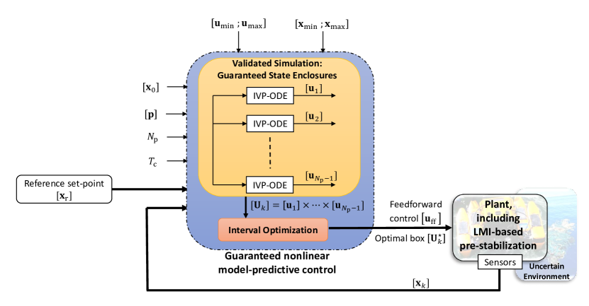
Figure 3. Overall structure of the interval-based nonlinear model predictive control approach, extended by an underlying pre-stabilization of the plant dynamics.

5. An Interval Observer-Based Approach for the Identification of the Open-Circuit Voltage Characteristic of Battery Cells

In this section, a continuous-time interval observer design is combined with a set-based identification of state-dependent output nonlinearities for the online-identification of the model of a Lithium-ion battery. According to [51], this approach makes use of an equivalent circuit model of the battery as described in [22].

In a first stage, the state variables of the system model

$$\dot{\mathbf{x}}(t) ={\mathbf{A}}\left({\sigma(t)}\right)\cdot{\mathbf{x}}(t)+{\mathbf{b}}\left({\sigma(t)}\right)\cdot u(t)$$ (56)

$$=\begin{bmatrix}0&0&0\\[2.84526pt] 0&\frac{-1}{{C}_{\mathrm{TS}}\left({\sigma(t)}\right)\cdot{R}_{\mathrm{TS}}\left({\sigma(t)}\right)}&0\\[2.84526pt] 0&0&\frac{-1}{{C}_{\mathrm{TL}}\left({\sigma(t)}\right)\cdot{R}_{\mathrm{TL}}\left({\sigma(t)}\right)}\\[2.84526pt] \end{bmatrix}\cdot{\textbf{x}}(t)+\begin{bmatrix}\frac{-1}{C_{\mathrm{Bat}}}\\[2.84526pt] \frac{1}{C_{\mathrm{TS}}\left({\sigma(t)}\right)}\\[2.84526pt] \frac{1}{C_{\mathrm{TL}}\left({\sigma(t)}\right)}\end{bmatrix}\cdot u(t)$$

with the state vector

$${\mathbf{x}}(t)=\begin{bmatrix}\sigma(t)&{v}_{\mathrm{TS}}(t)&{v}_{\mathrm{TL}}(t)\end{bmatrix}^{T}\enspace$$ (57)

are estimated. These state variables denote the state of charge of the battery as well as two voltages across resistor–capacitor sub-networks included in the equivalent circuit to represent delay phenomena between state-like changes of the terminal current and measurable variations of the terminal voltage. According to [51], interval enclosures of the state variables are estimated after reformulation of both the state equations (56) and the output equation

$$\tilde{v}_{\mathrm{OC}}(\sigma(t)) ={\mathbf{C}}\left({\sigma(t)}\right)\cdot{\mathbf{x}}(t)$$ (58)

$$=\eta_{\mathrm{OC}}\left({\sigma(t)}\right)\cdot\sigma(t)={v}_{\mathrm{OC}}(\sigma(t))-v_{0}-v_{2}$$ (59)

$$=\left({v_{0}\cdot\frac{e^{v_{1}\cdot\sigma(t)}-1}{\sigma(t)}+v_{3}+v_{4}\cdot\sigma(t)+v_{5}\cdot\sigma^{2}(t)}\right)\cdot\sigma(t)$$ (60)

in a quasi-linear form in which state of charge dependent matrices and vectors ${\mathbf{A}}\left({\sigma(t)}\right)$, ${\mathbf{b}}\left({\sigma(t)}\right)$, and ${\mathbf{C}}\left({\sigma(t)}\right)$, respectively, are separated from the state vector ${\mathbf{x}}(t)$ and the input variable $u(t)$, which is represented by the terminal current $i_{\mathrm{T}}$.

In a second stage, an interval-based set intersection approach is subsequently used to identify the unknown characteristic of the open circuit voltage ${v}_{\mathrm{OC}}(\sigma(t))$. This overall approach is summarized in Fig. 4.

For the observer design, cooperativity of the system model (as discussed in the introduction of this article) as well as stability of the estimation error dynamics are ensured by choosing the observer gain matrix $\mathbf{H}$ according to [29], in the form

$${\mathbf{H}}=\left[\begin{array}[]{ccc}h_{1}&0&0\\ \end{array}\right]^{T}$$ (61)

with $h_{1}>0$.

In such a way, interval bounds $\hat{\mathbf{x}}\in\left[{\hat{\mathbf{x}}}\right]:=\left[{\hat{\mathbf{\underline{x}}}}\;;\;{\hat{\mathbf{\overline{x}}}}\right]$ can be determined for the true, non-measurable state vector ${\mathbf{x}}$ by the decoupled lower and upper bounding systems [29, 63], following Müller’s theorem [58],

$$\underline{{\mathbf{A}}_{\mathrm{O}}\hat{\mathbf{{x}}}}+\underline{\mathbf{b}\mathbf{u}}+\mathbf{H}\underline{\mathbf{y}}_{\mathrm{m}}\leq\dot{\hat{\mathbf{x}}}\leq\overline{{\mathbf{A}}_{\mathrm{O}}\hat{\mathbf{{x}}}}+\overline{\mathbf{b}\mathbf{u}}+\mathbf{H}\overline{\mathbf{y}}_{\mathrm{m}}\enspace,~{}\hat{\mathbf{x}}\in\left[{\hat{\mathbf{x}}}\right]\enspace,$$ (62)

where

$${\mathbf{A}}_{\mathrm{O}}={\mathbf{A}}-\mathbf{H}\mathbf{C}\enspace\in\enspace\left[{\underline{\mathbf{A}}_{\mathrm{O}}}\;;\;{\overline{\mathbf{A}}_{\mathrm{O}}}\right]$$ (63)

is a Metzler matrix [27, 40, 36] with non-negative off-diagonal elements and

$$\left[{{\mathbf{y}}_{\mathrm{m}}}\right]:=\left[{\underline{\mathbf{y}}_{\mathrm{m}}}\;;\;{\overline{\mathbf{y}}_{\mathrm{m}}}\right]={\mathbf{y}}_{\mathrm{m}}+\left[{-\Delta{\mathbf{y}}_{\mathrm{m}}}\;;\;{\Delta{\mathbf{y}}_{\mathrm{m}}}\right]$$ (64)

is the measured system output with bounded uncertainty.

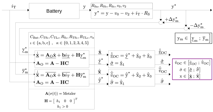
Figure 4. Estimation of the open-circuit voltage and the state of charge.

The estimated state of charge, enclosed by the interval $\left[{\hat{\sigma}}\right]$, together with the estimated open-circuit voltage

$$\tilde{v}_{\mathrm{OC}}(t)=\mathrm{y}^{*}_{\mathrm{m}}(t)+\hat{v}_{\mathrm{TS}}(t)+\hat{v}_{\mathrm{TL}}(t)\enspace,$$ (65)

with $\hat{v}_{\mathrm{TS}}(t)\in\left[{\hat{v}_{\mathrm{TS}}(t)}\right]$ and $\hat{v}_{\mathrm{TL}}(t)\in\left[{\hat{v}_{\mathrm{TL}}(t)}\right]$, allow for constructing the interval box $\left[{\mathbf{\Gamma}}\right]=\left[{\sigma(t)}\right]\times\left[{\tilde{v}_{\mathrm{OC}}(t)}\right]$ with $\sigma(t)\in\left[{\underline{\sigma}(t)}\;;\;{\overline{\sigma}(t)}\right]$ and $\tilde{v}_{\mathrm{OC}}(t)\in\left[{\underline{\tilde{v}}_{\mathrm{OC}}(t)}\;;\;{\overline{\tilde{v}}_{\mathrm{OC}}(t)}\right]$.

Successive intersections of these interval boxes — at different points in time — are utilized to improve the approximation of the true ${v}_{\mathrm{OC}}(\sigma(t))$ characteristic according to Figure 5.

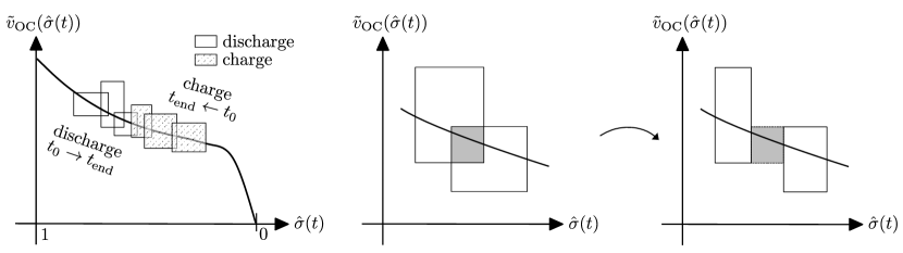
Figure 5. Identification of nonlinear dependencies using interval methods.

For strategies, allowing for a reduction of the computational complexity due to a large number of interval boxes to be intersected, the interval merging routine according to [46] is employed. Moreover, refinements of the estimated open-circuit voltage characteristic are possible by implementing a forward–backward contractor, as discussed from a methodological point of view in [34]. These refinements have been demonstrated recently in [50].

6. Combination of Set-Based and Stochastic Uncertainty Representations: An Application to Iterative-Learning Observer Design

In the final part of this article, a combination of stochastic and set-based (in this case, ellipsoidal) uncertainty representations is considered. This approach allows, on the one hand, for a rigorous quantification of predefined confidence levels in stochastic state estimation procedures. On the other hand, it allows for handling nonlinearities in such a way that the previously mentioned tolerance bounds are definitely not determined in an overly optimistic manner [68, 67, 81].

In addition to the properties mentioned above, we present a formulation of the state estimation procedure that allows to iteratively enhance the estimation accuracy for the case of periodically recurring trajectories and disturbance profiles (e.g., due to errors caused by a deterministic model mismatch due to purposefully performed model simplifications). For that purpose, assume the discrete time system model

$$\mathbf{z}_{k+1}=\boldsymbol{\Phi}\left({\mathbf{z}_{k},\mathbf{p}}\right)\cdot\mathbf{z}_{k}$$ (66)

with the bounded parameter vector $\mathbf{p}\in\left[{\underline{\mathbf{p}}}\;;\;{\overline{\mathbf{p}}}\right]$. As discussed in the following, the vector $\mathbf{z}_{k}\in\mathbb{R}^{\tilde{n}}$ consists of both system states and noise variables. Furthermore, assume that the ellipsoidal domain

$${\mathcal{E}}_{k}\left({\boldsymbol{\mu}_{k},\boldsymbol{\Gamma}_{k}^{\prime},r}\right)\\ :=\left\{\mathbf{z}_{k}\in\mathbb{R}^{n}\bigm{|}\left({\mathbf{z}_{k}-\boldsymbol{\mu}_{k}}\right)^{T}{\boldsymbol{\Gamma}_{k}^{\prime}}^{-T}{\boldsymbol{\Gamma}_{k}^{\prime}}^{-1}\left({\mathbf{z}_{k}-\boldsymbol{\mu}_{k}}\right)\leq r^{2}\right\}$$ (67)

specifies the confidence bound of a given percentage if the vector $\mathbf{z}_{k}$ is normally distributed with the positive definite covariance matrix $\mathbf{Q}_{k}^{\prime}=\boldsymbol{\Gamma}_{k}^{\prime}{\boldsymbol{\Gamma}_{k}^{\prime}}^{T}\succ 0$ and the ellipsoid midpoint (expected value) $\boldsymbol{\mu}_{k}\in\mathbb{R}^{\tilde{n}}$. Here, the parameter $r$ describes a magnification factor according to [92] associated with this confidence level.

6.1. Ellipsoidal Calculus for the Guaranteed Preduction of Covariance Ellipsoids

For the implementation of an ellipsoidal covariance prediction step (based on the references [65, 66, 71]), we use the definitions

$$\boldsymbol{\Gamma}_{k}:=r\cdot\boldsymbol{\Gamma}_{k}^{\prime}\quad\text{and}\quad\mathbf{Q}_{k}:=r^{2}\cdot\mathbf{Q}_{k}^{\prime}\enspace.$$ (68)

For the compactness of notation, reformulate the system model (66) into the form

$$\mathbf{z}_{k+1}=\boldsymbol{\Phi}\left({\mathbf{z}_{k},\mathbf{p}}\right)\cdot\check{\mathbf{z}}_{k}+\tilde{\boldsymbol{\Phi}}\cdot\boldsymbol{\mu}_{k}+\left({\boldsymbol{\Phi}\left({\mathbf{z}_{k},\mathbf{p}}\right)-\tilde{\boldsymbol{\Phi}}}\right)\cdot\boldsymbol{\mu}_{k}$$ (69)

with $\mathbf{z}_{k}=\check{\mathbf{z}}_{k}+\boldsymbol{\mu}_{k}$, where

$$\mathbf{z}_{k}\in{\mathcal{E}}_{k}={\mathcal{E}}_{k}\left({\boldsymbol{\mu}_{k},\boldsymbol{\Gamma}_{k}^{\prime},r}\right)\enspace.$$ (70)

Here, ${\mathcal{E}}_{k}$ denotes the uncertainty on the non-origin centered states $\mathbf{z}_{k}$,

$$\check{\mathbf{z}}_{k}\in\check{{\mathcal{E}}}_{k}=\check{{\mathcal{E}}}_{k}\left({\mathbf{0},\boldsymbol{\Gamma}_{k}^{\prime},r}\right)$$ (71)

the uncertainty on $\check{\mathbf{z}}_{k}$ after shifting the ellipsoid to the origin, and

$$\tilde{\boldsymbol{\Phi}}=\boldsymbol{\Phi}\left({\boldsymbol{\mu}_{k},\mathrm{mid}\left({\left[{\mathbf{p}}\right]}\right)}\right)$$ (72)

is the midpoint approximation of the quasi-linear system matrix with

$$\mathrm{mid}\left({\left[{\mathbf{p}}\right]}\right)=\frac{1}{2}\cdot\left({\underline{\mathbf{p}}+\overline{\mathbf{p}}}\right)\enspace.$$ (73)

Let also $\square{\mathcal{E}_{k}}$ denote an axis-aligned enclosure of ${\mathcal{E}}_{k}$ in the form of an $\tilde{n}$-dimensional interval box. An alternative to the definition (72) is given by

$$\tilde{\boldsymbol{\Phi}}=\mathrm{mid}\left({\boldsymbol{\Phi}\left({\square{\mathcal{E}_{k}},\left[{\mathbf{p}}\right]}\right)}\right)\enspace,$$ (74)

which is preferable if (72) and (74) strongly differ from each other in the case of large uncertainty.

Then, a confidence bound of the predicted states $\mathbf{z}_{k+1}$ of magnification $r$ is given by the ellipsoid ${\mathcal{E}}_{k+1}\left({\boldsymbol{\mu}_{k+1},\boldsymbol{\Gamma}_{k+1}^{\prime},r}\right)$ with the covariance $\mathbf{Q}_{k+1}^{\prime}=\boldsymbol{\Gamma}_{k+1}^{\prime}\left({{\boldsymbol{\Gamma}_{k+1}^{\prime}}}\right)^{T}$ for which the parameters are computed in the following steps.

P1:

Apply

$$\check{\mathbf{z}}_{k+1}=\boldsymbol{\Phi}\left({\mathbf{z}_{k},\mathbf{p}}\right)\cdot\check{\mathbf{z}}_{k}$$ (75)

to the ellipsoid $\check{{\mathcal{E}}}_{k}$ in (71). The outer ellipsoid enclosure of the image set is described by an ellipsoid with the shape matrix

$$\check{\mathbf{Q}}_{k+1}=\alpha_{k+1}^{2}\cdot\boldsymbol{\Gamma}_{k+1}\cdot\boldsymbol{\Gamma}_{k+1}^{T}\enspace,$$ (76)

where $\alpha_{k+1}\geq 0$ is the smallest value for which the LMI

is satisfied for all $\mathbf{z}_{k}\in\square{\mathcal{E}_{k}}$ and $\mathbf{p}\in\left[{\mathbf{p}}\right]$ with

$$\mathbcal{R}_{k}:=\boldsymbol{\Gamma}_{k}\cdot\boldsymbol{\Gamma}_{k}^{T}\enspace.$$ (78)

In (77), the symbol $\preceq$ denotes the negative semi-definiteness of the corresponding matrix expression and $\boldsymbol{\Lambda}$ is a preconditioning matrix chosen according to [66].

P2:

Compute interval bounds for the term

$$\mathbf{b}_{k}=\left({\boldsymbol{\Phi}\left({\mathbf{p}}\right)-\tilde{\boldsymbol{\Phi}}}\right)\cdot\boldsymbol{\mu}_{k}\in\left[{\mathbf{b}_{k}}\right]$$ (79)

which accounts for a non-zero ellipsoid midpoint with $\mathbf{z}_{k}$, $\tilde{\boldsymbol{\Phi}}$, and $\mathbf{p}$ defined according to (70), (72), and (73). Inflate the ellipsoid bound described by the shape matrix (76) according to [71]

$${\mathbf{Q}}_{k+1} =\left({1+\rho_{\mathrm{O},k+1}}\right)^{2}\cdot\check{\mathbf{Q}}_{k+1}~{},$$ (80)

$$\rho_{\mathrm{O},k+1} =\sup\left\{\left\|\alpha_{k+1}^{-1}\cdot\boldsymbol{\Gamma}_{k}^{-1}\cdot\left[{\mathbf{b}_{k}}\right]\right\|\right\}\enspace.$$ (81)

P3:

Compute the updated ellipsoid midpoint

$$\boldsymbol{\mu}_{k+1}=\tilde{\boldsymbol{\Phi}}\cdot\boldsymbol{\mu}_{k}$$ (82)

and its factorized shape matrix

$$\begin{split}\boldsymbol{\Gamma}_{k+1}^{\prime}=\alpha_{k+1}\cdot\left({1+\rho_{\mathrm{O},k+1}}\right)\cdot\tilde{\boldsymbol{\Phi}}\cdot\boldsymbol{\Gamma}_{k}^{\prime}\,.\end{split}$$ (83)

6.2. Stochastic Iterative-Learning Observer Design for Quasi-Linear State Equations

Consider the quasi-linear discrete-time state-space representation

$$\begin{split}\mathbf{x}_{k+1}&=\mathbf{A}\left({{\mathbf{x}}_{k},\mathbf{p}}\right)\cdot\mathbf{x}_{k}+\mathbf{E}\left({{\mathbf{x}}_{k},\mathbf{p}}\right)\cdot\mathbf{w}_{k}\\ \mathbf{y}_{k}&=\mathbf{C}\left({{\mathbf{x}}_{k},\mathbf{p}}\right)\cdot\mathbf{x}_{k}+\mathbf{v}_{k}\end{split}$$ (84)

with the state vector $\mathbf{x}_{k}\in\mathbb{R}^{n}$, the measured output vector $\mathbf{y}_{k}\in\mathbb{R}^{m}$ ($m\leq n$), as well as the uncorrelated process and measurement noise vectors $\mathbf{w}_{k}\in\mathbb{R}^{n_{\mathbf{w}}}$ and $\mathbf{v}_{k}\in\mathbb{R}^{n_{\mathbf{v}}}$, respectively. Let both noise vectors be normally distributed with the covariances $\mathbf{C}_{\mathbf{w},k}$ and $\mathbf{C}_{\mathbf{v},k}$ and vanishing mean. The iterative-learning observer is designed in this section to estimate the state vector $\mathbf{x}_{k}$ as well as its uncertainty (expressed by its covariance) by a Kalman Filter-like procedure. This estimator does not only operate along the time domain $k$ but also enhances the estimates successively from the trial $i$ to the trial $i+1$. Moreover, to allow for the identification of a systematic model mismatch, a lumped correction term $\boldsymbol{\delta}_{k}$ is added to the state equations (84) in the form

$$\mathbf{x}_{k+1}=\mathbf{A}\left({{\mathbf{x}}_{k},\mathbf{p}}\right)\cdot\mathbf{x}_{k}+\mathbf{E}\left({{\mathbf{x}}_{k},\mathbf{p}}\right)\cdot\mathbf{w}_{k}+\boldsymbol{\delta}_{k}\enspace.$$ (85)

For the derivation of the learning-type framework, consider the trials $\xi=i$ and $\xi=i+1$ with the actually measured data $\mathbf{y}_{\mathrm{m},k}^{\xi}=\mathbf{C}_{k}^{\xi}\cdot\mathbf{x}_{k}^{\xi}+\mathbf{v}_{k}^{\xi}$ corresponding to the realizations of the general outputs $\mathbf{y}_{k}$ in (84) for these two trials.

For the recursive formulation of the iterative-learning observer, we assume that both process and measurement noise are uncorrelated and normally distributed with zero mean. The superscript $\mathrm{p}$ denotes the result of the prediction step, while the superscript $\mathrm{e}$ refers to the estimation result as the outcome of the measurement-based innovation step.

6.2.1. Prediction Step for State- and Parameter-Dependent Disturbance Inputs $\mathbf{E}\left({{\mathbf{x}}_{k},\mathbf{p}}\right)$ [67]

Define an ellipsoid for the augmented state vector

$$\mathbf{z}_{k}=\begin{bmatrix}\left({\mathbf{x}_{k}^{i}}\right)^{T}&\left({\mathbf{x}_{k}^{i+1}}\right)^{T}&\left({\mathbf{w}_{k}^{i}}\right)^{T}&\left({\mathbf{w}_{k}^{i+1}}\right)^{T}\end{bmatrix}^{T}$$ (86)

corresponding to the result of the preceding innovation step, augmented by the influence of the uncorrelated process noise in both trials $i$ and $i+1$ in the form

$$\mathcal{E}_{k}^{\mathrm{e},i|i+1}\left({\begin{bmatrix}\boldsymbol{\mu}_{k}^{\mathrm{e},i}\\ \boldsymbol{\mu}_{k}^{\mathrm{e},i+1}\\ \mathbf{0}\\ \mathbf{0}\end{bmatrix},\boldsymbol{\Gamma}_{k}^{\mathrm{e}},r}\right)$$ (87)

with

$$\boldsymbol{\Gamma}_{k}^{\mathrm{e}}=\begin{bmatrix}\boldsymbol{\Gamma}_{k}^{\mathrm{e},i|i+1}&\mathbf{0}_{2n\times 2n_{\mathbf{w}}}\\ \mathbf{0}_{2n_{\mathbf{w}}\times 2n}&\begin{bmatrix}\mathbf{C}_{\mathbf{w},k}&\mathbf{0}\\ \mathbf{0}&\mathbf{C}_{\mathbf{w},k}\end{bmatrix}^{\frac{1}{2}}\end{bmatrix}$$ (88)

containing the matrix square root $\boldsymbol{\Gamma}_{k}^{\mathrm{e},i|i+1}$ of the combined state covariance matrix

$$\mathbf{C}_{k}^{\mathrm{e},i|i+1}=\boldsymbol{\Gamma}_{k}^{\mathrm{e},i|i+1}\cdot\left({\boldsymbol{\Gamma}_{k}^{\mathrm{e},i|i+1}}\right)^{T}$$ (89)

as well as of the iteration-independent noise covariance $\mathbf{C}_{\mathbf{w},k}$, and the magnification factor $r\geq 1$ as a user-defined degree of freedom.

Then, the application of the system model

$$\boldsymbol{\Phi}\left({\mathbf{z}_{k},\mathbf{p}}\right)=\begin{bmatrix}\mathbf{A}\left({{\mathbf{x}}_{k}^{i},\mathbf{p}}\right)&\mathbf{0}_{n\times n}&\mathbf{E}\left({{\mathbf{x}}_{k}^{i},\mathbf{p}}\right)&\mathbf{0}_{n\times n_{\mathbf{w}}}\\ \mathbf{0}_{n\times n}&\mathbf{A}\left({{\mathbf{x}}_{k}^{i+1},\mathbf{p}}\right)&\mathbf{0}_{n\times n_{\mathbf{w}}}&\mathbf{E}\left({{\mathbf{x}}_{k}^{i+1},\mathbf{p}}\right)\\ \mathbf{0}_{n_{\mathbf{w}}\times n}&\mathbf{0}_{n_{\mathbf{w}}\times n}&\mathbf{I}_{n_{\mathbf{w}}\times n_{\mathbf{w}}}&\mathbf{0}_{n_{\mathbf{w}}\times n_{\mathbf{w}}}\\ \mathbf{0}_{n_{\mathbf{w}}\times n}&\mathbf{0}_{n_{\mathbf{w}}\times n}&\mathbf{0}_{n_{\mathbf{w}}\times n_{\mathbf{w}}}&\mathbf{I}_{n_{\mathbf{w}}\times n_{\mathbf{w}}}\\ \end{bmatrix}$$ (90)

to the ellipsoid (87) according to Sec. 6.1 yields the ellipsoid

$$\mathcal{E}_{k+1}^{\mathrm{p},i|i+1}\left({\begin{bmatrix}\boldsymbol{\mu}_{k+1}^{\mathrm{p},i}\\ \boldsymbol{\mu}_{k+1}^{\mathrm{p},i+1}\\ \mathbf{0}\\ \mathbf{0}\end{bmatrix},\boldsymbol{\Gamma}_{k+1}^{\mathrm{p}},r}\right)$$ (91)

in which the first $2n$ components of the midpoint represent the predicted expected value vector $\begin{bmatrix}\left({\boldsymbol{\mu}_{k+1}^{\mathrm{p},i}}\right)^{T}&\left({\boldsymbol{\mu}_{k+1}^{\mathrm{p},i+1}}\right)^{T}\end{bmatrix}^{T}$ and the covariance $\mathbf{C}_{k+1}^{\mathrm{p},i|i+1}$ is obtained by extracting the upper left $(2n\times 2n)$ block of the matrix product $\boldsymbol{\Gamma}_{k+1}^{\mathrm{p}}\cdot\left({\boldsymbol{\Gamma}_{k+1}^{\mathrm{p}}}\right)^{T}$. For the simplified case, in which the disturbance input matrix $\mathbf{E}$ is constant, the reader is referred to [67].

6.2.2. Innovation Step

The measurement-based innovation step makes use of the deviations

$$\Delta\mathbf{y}_{k}^{i} ={\mathbf{y}_{\mathrm{m},k}^{i}-\mathbf{C}_{k}^{i}\cdot\boldsymbol{\mu}_{k}^{\mathrm{p},i}}$$ (92)

and

$$\Delta\mathbf{y}_{k}^{i+1} ={\mathbf{y}_{\mathrm{m},k}^{i+1}-\mathbf{C}_{k}^{i+1}\cdot\boldsymbol{\mu}_{k}^{\mathrm{p},i+1}}$$ (93)

between the measured data in the trials $i$ and $i+1$, respectively, and the corresponding output forecasts based on the prediction step of the previous subsection. Using these output deviations, and assuming the standard detectability requirements of the Kalman Filter design to be satisfied, the expected values are updated according to [68] by

$$\begin{bmatrix}\boldsymbol{\mu}_{k}^{\mathrm{e},i}\\ \boldsymbol{\mu}_{k}^{\mathrm{e},i+1}\end{bmatrix}=\begin{bmatrix}\boldsymbol{\mu}_{k}^{\mathrm{p},i}\\ \boldsymbol{\mu}_{k}^{\mathrm{p},i+1}\end{bmatrix}+\tilde{\mathbf{H}}_{k}\cdot\begin{bmatrix}\mathbf{y}_{\mathrm{m},k}^{i}\\ \mathbf{y}_{\mathrm{m},k}^{i+1}\end{bmatrix}-\tilde{\mathbf{H}}_{k}\tilde{\mathbf{C}}_{k}\cdot\begin{bmatrix}\boldsymbol{\mu}_{k}^{\mathrm{p},i}\\ \boldsymbol{\mu}_{k}^{\mathrm{p},i+1}\end{bmatrix}\enspace,$$ (94)

where the combined output matrix

$$\tilde{\mathbf{C}}_{k}:=\begin{bmatrix}\mathbf{C}_{k}^{i}&\mathbf{0}\\ \mathbf{0}&\mathbf{C}_{k}^{i+1}\end{bmatrix}$$ (95)

results from pointwise evaluations of the quasi-linear system’s output matrix according to

$$\mathbf{C}_{k}^{i} :=\mathbf{C}_{k}\left({\boldsymbol{\mu}_{k}^{\mathrm{p},i},\mathrm{mid}\left({\left[{\mathbf{p}}\right]}\right)}\right)$$ (96)

and

$$\mathbf{C}_{k}^{i+1} :=\mathbf{C}_{k}\left({\boldsymbol{\mu}_{k}^{\mathrm{p},i+1},\mathrm{mid}\left({\left[{\mathbf{p}}\right]}\right)}\right)\enspace$$ (97)

The corresponding estimation error covariance is, then, given as

$$\mathbf{C}_{k}^{\mathrm{e},i|i+1} =\mathrm{E}\left\{\begin{bmatrix}\mathbf{x}_{k}^{i}-\boldsymbol{\mu}_{k}^{\mathrm{e},i}\\ \mathbf{x}_{k}^{i+1}-\boldsymbol{\mu}_{k}^{\mathrm{e},i+1}\end{bmatrix}\cdot\begin{bmatrix}\mathbf{x}_{k}^{i}-\boldsymbol{\mu}_{k}^{\mathrm{e},i}\\ \mathbf{x}_{k}^{i+1}-\boldsymbol{\mu}_{k}^{\mathrm{e},i+1}\end{bmatrix}^{T}\right\}$$

$$=\mathrm{Cov}\left\{\begin{bmatrix}\mathbf{x}_{k}^{i}-\boldsymbol{\mu}_{k}^{\mathrm{e},i}\\ \mathbf{x}_{k}^{i+1}-\boldsymbol{\mu}_{k}^{\mathrm{e},i+1}\end{bmatrix}\right\}$$

$$=\mathbf{M}_{k}\mathbf{C}_{k}^{\mathrm{p},i|i+1}\mathbf{M}_{k}^{T}+\tilde{\mathbf{H}}_{k}\tilde{\mathbf{C}}_{\mathbf{v},k}\tilde{\mathbf{H}}_{k}^{T}\enspace,$$ (98)

where

$$\mathbf{M}_{k}=\begin{bmatrix}\mathbf{I}&\mathbf{0}\\ \mathbf{0}&\mathbf{I}\end{bmatrix}-\tilde{\mathbf{H}}_{k}\tilde{\mathbf{C}}_{k}$$ (99)

and

$$\tilde{\mathbf{H}}_{k}:=\begin{bmatrix}\mathbf{H}_{1,k}^{i+1}&\mathbf{0}\\ \mathbf{H}_{2,k}^{i+1}&\mathbf{H}_{1,k}^{i+1}-\mathbf{H}_{2,k}^{i+1}\end{bmatrix}\enspace.$$ (100)

As shown in [68], the estimation error covariance is minimized by the filter gain matrices $\mathbf{H}_{1,k}^{i+1}$ and $\mathbf{H}_{2,k}^{i+1}$ that are derived in the following, where the predicted covariance is partitioned in a blockwise manner according to

$$\mathbf{C}_{k}^{\mathrm{p},i|i+1}=\begin{bmatrix}\mathbf{C}_{\mathrm{A},k}^{\mathrm{p}}&\mathbf{C}_{\mathrm{B},k}^{\mathrm{p}}\\ \star&\mathbf{C}_{\mathrm{C},k}^{\mathrm{p}}\end{bmatrix}\enspace,$$ (101)

and $\star$ denotes blocks that can be inferred from the symmetry of the result. Moreover, the residual covariance is defined as

$$\mathbf{P}\cdot{\tilde{\boldsymbol{\Gamma}}_{k}^{\mathrm{e}}\cdot\left({\tilde{\boldsymbol{\Gamma}}_{k}^{\mathrm{e}}}\right)^{T}}\cdot\mathbf{P}^{T}+\tilde{\mathbf{C}}_{\mathbf{v},k}=\begin{bmatrix}\mathbf{C}_{\mathrm{A},k}&\mathbf{C}_{\mathrm{B},k}\\ \star&\mathbf{C}_{\mathrm{C},k}\end{bmatrix}$$ (102)

with the projection matrix $\mathbf{P}=\begin{bmatrix}\mathbf{I}_{m\times m}&\mathbf{0}_{m\times(n-m)}\end{bmatrix}$ and the trial-independent measurement noise covariance

$$\tilde{\mathbf{C}}_{\mathbf{v},k}:=\begin{bmatrix}{\mathbf{C}}_{\mathbf{v},k}&\mathbf{0}\\ \mathbf{0}&{\mathbf{C}}_{\mathbf{v},k}\end{bmatrix}\enspace.$$ (103)

As a specific feature introduced in [67], aiming at a robustification of the innovation stage against nonlinearities, the matrix $\tilde{\boldsymbol{\Gamma}}_{k}^{\mathrm{e}}$ is obtained by the consideration of the quasi-linearity of the output equation with the help of the ellipsoid

$$\mathcal{E}_{k}^{\mathrm{p},i|i+1}\left({\begin{bmatrix}\boldsymbol{\mu}_{k}^{\mathrm{p},i}\\ \boldsymbol{\mu}_{k}^{\mathrm{p},i+1}\end{bmatrix},\boldsymbol{\Gamma}_{k}^{\mathrm{p},i|i+1},r}\right)$$ (104)

that is propagated through a quasi-linear system model in the form (66) with the associated system matrix ($\mathbf{y}_{\mathrm{m},k}^{i},\mathbf{y}_{\mathrm{m},k}^{i+1}\in\mathbb{R}^{m}$)

$$\boldsymbol{\Phi}\left({\mathbf{z}_{k},\mathbf{p}}\right)=\begin{bmatrix}\mathbf{C}\left({{\mathbf{x}}_{k}^{i},\mathbf{p}}\right)&\mathbf{0}_{m\times n}\\ \mathbf{0}_{m\times n}&\mathbf{C}\left({{\mathbf{x}}_{k}^{i+1},\mathbf{p}}\right)\\ \begin{matrix}\mathbf{0}_{(n-m)\times m}&\mathbf{I}_{(n-m)\times(n-m)}\end{matrix}&\mathbf{0}_{(n-m)\times n}\\ \mathbf{0}_{(n-m)\times n}&\begin{matrix}\mathbf{0}_{(n-m)\times m}&\mathbf{I}_{(n-m)\times(n-m)}\end{matrix}\end{bmatrix}\enspace,$$ (105)

where $\boldsymbol{\Phi}\left({\mathbf{z}_{k},\mathbf{p}}\right)\in\mathbf{R}^{{2n}\times 2n}$. The evaluation of this quasi-linear model yields an ellipsoid

$$\mathcal{E}_{k}^{\mathrm{e}}\left({\tilde{\boldsymbol{\mu}}_{k}^{\mathrm{e}},\tilde{\boldsymbol{\Gamma}}_{k}^{\mathrm{e}},r}\right)$$ (106)

from which the associated shape matrix ${\tilde{\boldsymbol{\Gamma}}_{k}^{\mathrm{e}}\cdot\left({\tilde{\boldsymbol{\Gamma}}_{k}^{\mathrm{e}}}\right)^{T}}$ is computed in Eq. (102), followed by an extraction of the upper left ($2m\times 2m$) block that corresponds to the actually measured output quantities. This subblock extraction is performed by the multiplication with the projection matrix $\mathbf{P}$ in the first summand of Eq. (102).

The optimal iterative-learning observer gains, in the sense of a minimization of the estimation error covariance, jointly considering the trials $i$ and $i+1$ are given by

$$\begin{split}\left[\begin{array}[]{c;{2pt/2pt}c}\mathbf{H}_{1,k}^{i+1}&\mathbf{H}_{2,k}^{i+1}\end{array}\right]&=\left[\begin{array}[]{c;{2pt/2pt}c}\!\!\!\left({{\mathbf{C}_{k}^{i}}\mathbf{C}_{\mathrm{A},k}^{\mathrm{p}}+{\mathbf{C}_{k}^{i+1}}\mathbf{C}_{\mathrm{C},k}^{\mathrm{p}}}\right)^{T}\!\!&\!\!\left({{\mathbf{C}_k^{i}} {\mathbf{C}_{\mathrm{B},k}^\mathrm{p}} -{\mathbf{C}_k^{i+1}} {\mathbf{C}_{\mathrm{C},k}^\mathrm{p}} }\right)^T\!\!\!\end{array}\right]\\ &\qquad\phantom{=}\cdot\begin{bmatrix}\mathbf{C}_{\mathrm{A},k}+\mathbf{C}_{\mathrm{C},k}&\star\\ \mathbf{C}_{\mathrm{B},k}-\mathbf{C}_{\mathrm{C},k}&\mathbf{C}_{\mathrm{A},k}-\left({\mathbf{C}_{\mathrm{B},k}+\mathbf{C}_{\mathrm{B},k}^{T}}\right)+\mathbf{C}_{\mathrm{C},k}\end{bmatrix}^{-1}\!\!\!\!.\end{split}$$ (107)

For a proof of this expression for the filter gain matrices, see [68]. The reference [67] demonstrates the successful application of this iterative-learning observer for the state and disturbance estimation of a Lithium-ion battery with periodically recurring input current profiles. Compared to the work [68], where an Extended Kalman Filter methodology was used in the form of a point-valued linearization of the state and output equations during the covariance computation in the prediction and innovation stages, the combination with the ellipsoidal calculus allows for a significant improvement of the state estimation accuracy, also yielding significantly tighter uncertainty bounds.

7. Conclusions and Future Work

In this paper, a comprehensive overview of recent advances concerning the offline and online use of interval and other set-based approaches for control and state estimation has been given. We have equally addressed methodological approaches and selected fields of practical applications in our review, where we have put a focus on the tasks of parameter estimation, robust and model-predictive control, as well as state estimation procedures.

Future work will focus especially on widening the field of applications by an investigation of control and state estimation tasks for distributed and large-scale, interconnected systems with parameter uncertainty and disturbances that are, among others, omnipresent in control scenarios in the Industry 4.0 as well as in the domain of energy systems. To cope with such systems, we will focus especially on the development of decentralized techniques for the parameter identification of large-scale system models, which will again form the basis for control and state estimator design. Moreover, we will further develop approaches that allow for removing restrictive monotonicity assumptions as already shown in works such as [93, 43, 42].

References

- [1] J. Alexandre dit Sandretto and A. Chapoutot. DynIBEX: A differential constraint library for studying dynamical systems. In Conference on Hybrid Systems: Computation and Control (HSCC 2016), 2016.
- [2] J. Alexandre dit Sandretto and A. Chapoutot. Validated explicit and implicit Runge–Kutta methods. Reliable Computing, 22(1):79–103, Jul 2016.
- [3] J. Alexandre dit Sandretto, G. Trombettoni, D. Daney, and G. Chabert. Certified calibration of a cable-driven robot using interval contractor programming. In F. Thomas, editor, Computational Kinematics, volume 15 of Mechanisms and Machine Science Ser, pages 209–217. Springer, The Netherlands, Dordrecht, 2014.
- [4] M. Althoff. An introduction to CORA 2015. In G. Frehse and M. Althoff, editors, ARCH14-15. 1st and 2nd International Workshop on Applied veRification for Continuous and Hybrid Systems, volume 34 of EPiC Series in Computing, pages 120–151. EasyChair, 2015. https://easychair.org/publications/paper/xMm, accessed: Sept. 1, 2023.
- [5] M. Althoff and B.H. Krogh. Zonotope bundles for the efficient computation of reachable sets. In 2011 50th IEEE Conference on Decision and Control and European Control Conference, pages 6814–6821, 2011.
- [6] D. Angeli and E.D. Sontag. Monotone control systems. IEEE Transactions on Automatic Control, 48(10):1684–1698, 2003.
- [7] E. Auer, A. Rauh, E. P. Hofer, and W. Luther. Validated modeling of mechanical systems with SmartMOBILE: Improvement of performance by ValEncIA-IVP. In Proc. of Dagstuhl Seminar 06021: Reliable Implementation of Real Number Algorithms: Theory and Practice, Lecture Notes in Computer Science, pages 1–27, 2008.
- [8] E. Auer, A. Rauh, and J. Kersten. Experiments-based parameter identification on the GPU for cooperative systems. Journal of Computational and Applied Mathematics, 371:112657, 2020.
- [9] Y. Becis-Aubry. Ellipsoidal constrained state estimation in presence of bounded disturbances. In Proc. of the 2021 European Control Conference (ECC), pages 555–560, Delft, The Netherlands, 2021.
- [10] S. Boyd, L. El Ghaoui, E. Feron, and V. Balakrishnan. Linear Matrix Inequalities in System and Control Theory. SIAM, Philadelphia, 1994.
- [11] F. Bünger. Shrink wrapping for Taylor models revisited. Numerical Algorithms, 78:1001–1017, 08 2018.
- [12] F. Bünger. A Taylor model toolbox for solving ODEs implemented in MATLAB/INTLAB. Journal of Computational and Applied Mathematics, 368:112511, 2020.
- [13] F. Bünger. Preconditioning of Taylor models, implementation and test cases. Nonlinear Theory and Its Applications, IEICE, 12(1):2–40, 2021.
- [14] H. Cornelius and R. Lohner. Computing the range of values of real functions with accuracy higher than second order. Computing, 33:331–347, 1984.
- [15] T. Csendes and D. Ratz. Subdivision direction selection in interval methods for global optimization. SIAM Journal on Numerical Analysis, 34(3):922–938, 1997.
- [16] A. dos Reis de Souza, D. Efimov, and T. Raïssi. Robust output feedback model predictive control of time-delayed systems using interval observers. International Journal of Robust and Nonlinear Control, 32(3):1180–1193, 2022.
- [17] A. dos Reis de Souza, D. Efimov, and T. Raïssi. Robust output feedback mpc for lpv systems using interval observers. IEEE Transactions on Automatic Control, 67(6):3188–3195, 2022.
- [18] A. dos Reis de Souza, D. Efimov, T. Raïssi, and X. Ping. Robust output feedback model predictive control for constrained linear systems via interval observers. Automatica, 135:109951, 2022.
- [19] T. Dötschel, E. Auer, A. Rauh, and H. Aschemann. Thermal behavior of high-temperature fuel cells: Reliable parameter identification and interval-based sliding mode control. Soft Computing, 17(8):1329–1343, 2013.
- [20] D. Efimov, T. Raïssi, S. Chebotarev, and A. Zolghadri. Interval state observer for nonlinear time varying systems. Automatica, 49(1):200–205, 2013.
- [21] İ Eker. Second-order sliding mode control with experimental application. ISA Transactions, 49(3):394–405, 2010.
- [22] O. Erdinç, B. Vural, and M. Uzunoğlu. A dynamic Lithium-ion battery model considering the effects of temperature and capacity fading. In Proc. of International Conference on Clean Electrical Power (ICCEP), pages 383–386. IEEE, 2009.
- [23] M. Fliess, J. Lévine, P. Martin, and P. Rouchon. Flatness and defect of nonlinear systems: Introductory theory and examples. International Journal of Control, 61:1327–1361, 1995.
- [24] M. Fnadi and J. Alexandre dit Sandretto. Experimental validation of a guaranteed nonlinear model predictive control. Algorithms, 14(8):248, 2021.
- [25] M. Fnadi and A. Rauh. Exponential state enclosure techniques for the implementation of validated model predictive control. Acta Cybernetica, 2023. Accepted for publication.
- [26] L. Fridman and A. Levant. Higher order sliding modes. In J.P. Barbot and W. Perruguetti, editors, Sliding Mode Control in Engineering, pages 53–101. Marcel Dekker, New York, 2002.
- [27] M. Gennat and B. Tibken. Computing guaranteed bounds for uncertain cooperative and monotone nonlinear systems. In Proc. of the 17th IFAC World Congress, pages 4846–4851. IFAC Proceedings Volumes, 2008.
- [28] O. Heimlich. Octave forge interval, 2018. https://wiki.octave.org/wiki/index.php?title=Interval_package&oldid=12214, version: 3.2.0, acessed: Sept. 01, 2023.
- [29] E. Hildebrandt, J. Kersten, A. Rauh, and H. Aschemann. Robust interval observer design for fractional-order models with applications to state estimation of batteries. In Proc. of the 21st IFAC World Congress, pages 3683–3688. IFAC-PapersOnLine, 2020.
- [30] M. Hirsch. On the nonchaotic nature of monotone dynamical systems. European Journal of Pure and Applied Mathematics, 12:680–688, 07 2019.
- [31] J. Hoefkens. Rigorous Numerical Analysis with High-Order Taylor Models. PhD thesis, Michigan State University, 2001. https://groups.nscl.msu.edu/nscl_library/Thesis/Hoefkens,%20Jens.pdf (accessed: Aug. 11, 2023).
- [32] S. Ifqir, V. Puig, D. Ichalal, N. Ait-Oufroukh, and S. Mammar. Zonotopic set-membership state estimation for switched systems. Journal of the Franklin Institute, 359(16):9241–9270, 2022.
- [33] L. Jaulin. Robust set-membership state estimation; application to underwater robotics. Automatica, 45(1):202–206, 2009.
- [34] L. Jaulin, M. Kieffer, O. Didrit, and É. Walter. Applied Interval Analysis. Springer–Verlag, London, 2001.
- [35] S.J. Julier, J.K. Uhlmann, and H.F. Durrant-Whyte. A new approach for the nonlinear transformation of means and covariances in filters and estimators. IEEE Transactions on Automatic Control, 45(3):477–482, 2000.
- [36] T. Kaczorek. Positive 1D and 2D Systems. Springer–Verlag, London, 2002.
- [37] R.E. Kalman. A new approach to linear filtering and prediction problems. Transaction of the ASME – Journal of Basic Engineering, 82(Series D):35–45, 1960.
- [38] T. Kapela, M. Mrozek, D. Wilczak, and P. Zgliczynski. CAPD::DynSys: A flexible C++ toolbox for rigorous numerical analysis of dynamical systems. Communications in Nonlinear Science and Numerical Simulation, page 105578, 11 2020.
- [39] J. Kersten, A. Rauh, and H. Aschemann. State-space transformations of uncertain systems with purely real and conjugate-complex eigenvalues into a cooperative form. In Proc. of 23rd Intl. Conf. on Methods and Models in Automation and Robotics 2018, Miedzyzdroje, Poland, 2018.
- [40] J. Kersten, A. Rauh, and H. Aschemann. Transformation of uncertain linear fractional order differential equations into a cooperative form. In Proc. of the 11th IFAC Symposium on Nonlinear Control Systems (NOLCOS), pages 646–651. IFAC-PapersOnLine, 2019.
- [41] J. Kersten, A. Rauh, and H. Aschemann. Interval methods for robust gain scheduling controllers: An lmi-based approach. Granular Computing, pages 203–216, 2020.
- [42] M. Khajenejad, F. Shoaib, and S.Z. Yong. Interval observer synthesis for locally lipschitz nonlinear dynamical systems via mixed-monotone decompositions. In 2022 American Control Conference (ACC), pages 2970–2975, 2022.
- [43] M. Khajenejad and S.Z. Yong. Tight remainder-form decomposition functions with applications to constrained reachability and guaranteed state estimation. IEEE Transactions on Automatic Control, pages 1–16, 2023.
- [44] A. Der Kiureghian and O. Ditlevsen. Aleatory or epistemic? Does it matter? Structural Safety, 31(2):105–112, 2009. Risk Acceptance and Risk Communication.
- [45] W. Krämer. XSC Languages (C-XSC, PASCAL-XSC) — Scientific computing with validation, arithmetic requirements, hardware solution and language support, 2012. www.math.uni-wuppertal.de/~xsc/, C-XSC 2.5.3, acessed: Sept. 01, 2023.
- [46] I. Krasnochtanova, A. Rauh, M. Kletting, H. Aschemann, E.P. Hofer, and K.-M. Schoop. Interval methods as a simulation tool for the dynamics of biological wastewater treatment processes with parameter uncertainties. Applied Mathematical Modeling, 34(3):744–762, 2010.
- [47] R. Krawczyk. Newton-Algorithmen zur Bestimmung von Nullstellen mit Fehlerschranken. Computing, 4:189–201, 1969. In German.
- [48] W. Kühn. Rigorous error bounds for the initial value problem based on defect estimation. Technical report, 1999. http://www.decatur.de/personal/papers/defect.zip (accessed: Sept. 1, 2021).
- [49] A.B. Kurzhanskii and I. Vályi. Ellipsoidal Calculus for Estimation and Control. Birkhäuser, Boston, MA, 1997.
- [50] M. Lahme and A. Rauh. Online identification of the open-circuit voltage characteristic of Lithium-ion batteries with a contractor-based procedure. In IEEE International Conference on Methods and Models in Automation and Robotics MMAR, Miedzyzdroje, Poland, 2023.
- [51] M. Lahme and A. Rauh. Set-valued approach for the online identification of the open-circuit voltage of Lithium-ion batteries. Acta Cybernetica, 2023. Accepted for publication.
- [52] Y. Lin and M.A. Stadtherr. Validated solutions of initial value problems for parametric ODEs. Applied Numerical Mathematics, 57(10):1145–1162, 2007.
- [53] R. Lohner. Enclosing the solutions of ordinary initial and boundary value problems. In E.W. Kaucher, U.W. Kulisch, and C. Ullrich, editors, Computer Arithmetic: Scientific Computation and Programming Languages, pages 255–286, Stuttgart, 1987. Wiley-Teubner Series in Computer Science.
- [54] H.J. Marquez. Nonlinear Control Systems. John Wiley & Sons, Inc., New Jersey, 2003.
- [55] G. Mayer. Interval Analysis and Automatic Result Verification. De Gruyter Studies in Mathematics. De Gruyter, Berlin/Boston, 2017.
- [56] F. Mazenc and O. Bernard. Asymptotically stable interval observers for planar systems with complex poles. IEEE Transactions on Automatic Control, 55(2):523–527, 2010.
- [57] R.E. Moore. Interval Arithmetic. Prentice-Hall, Englewood Cliffs, N.J., 1966.
- [58] M. Müller. Über die Eindeutigkeit der Integrale eines Systems gewöhnlicher Differenzialgleichungen und die Konvergenz einer Gattung von Verfahren zur Approximation dieser Integrale. In Sitzungsbericht Heidelberger Akademie der Wissenschaften, 1927.
- [59] N.S. Nedialkov. Computing Rigorous Bounds on the Solution of an Initial Value Problem for an Ordinary Differential Equation. PhD thesis, Graduate Department of Computer Science, University of Toronto, 1999.
- [60] N.S. Nedialkov. Interval tools for ODEs and DAEs. In CD-Proc. of 12th GAMM-IMACS Intl. Symposium on Scientific Computing, Computer Arithmetic, and Validated Numerics SCAN 2006, Duisburg, Germany, 2007. IEEE Computer Society.
- [61] N.S. Nedialkov. Implementing a rigorous ode solver through literate programming. In A. Rauh and E. Auer, editors, Modeling, Design, and Simulation of Systems with Uncertainties, Mathematical Engineering, pages 3–19. Springer, Berlin, Heidenberg, 2011.
- [62] A. Neumaier. Interval Methods for Systems of Equations. Cambridge University Press, Encyclopedia of Mathematics, Cambridge, 1990.
- [63] T. Raïssi and D. Efimov. Some recent results on the design and implementation of interval observers for uncertain systems. at-Automatisierungstechnik, 66(3):213–224, 2018.
- [64] T. Raïssi, D. Efimov, and A. Zolghadri. Interval state estimation for a class of nonlinear systems. IEEE Trans. Automat. Contr., 57:260–265, 2012.
- [65] A. Rauh, A. Bourgois, and L. Jaulin. Union and intersection operators for thick ellipsoid state enclosures: Application to bounded-error discrete-time state observer design. Algorithms, 14(3):88, 2021.
- [66] A. Rauh, A. Bourgois, L. Jaulin, and J. Kersten. Ellipsoidal enclosure techniques for a verified simulation of initial value problems for ordinary differential equations. In Proc. of 5th International Conference on Control, Automation and Diagnosis (ICCAD’21), Grenoble, France, 2021.
- [67] A. Rauh, T. Chevet, T.N. Dinh, J. Marzat, and T. Raïssi. Robust iterative learning observers based on a combination of stochastic estimation schemes and ellipsoidal calculus. In 25th International Conference on Information Fusion (FUSION), pages 1–8, Linköping, Sweden, 2022.
- [68] A. Rauh, T. Chevet, T.N. Dinh, J. Marzat, and T. Raïssi. A stochastic design approach for iterative learning observers for the estimation of periodically recurring trajectories and disturbances. In Proc. of the 20th European Control Conference ECC, London, UK, 2022.
- [69] A. Rauh, T. Dötschel, and H. Aschemann. Experimental parameter identification for a control-oriented model of the thermal behavior of high-temperature fuel cells. In CD-Proc. of IEEE International Conference on Methods and Models in Automation and Robotics MMAR, Miedzyzdroje, Poland, 2011.
- [70] A. Rauh and E. P. Hofer. Interval methods for optimal control. In A. Frediani and G. Buttazzo, editors, Proceedings of the 47th Workshop on Variational Analysis and Aerospace Engineering 2007, pages 397–418, School of Mathematics, Erice, Italy, 2009. Springer–Verlag.
- [71] A. Rauh and L. Jaulin. A computationally inexpensive algorithm for determining outer and inner enclosures of nonlinear mappings of ellipsoidal domains. International Journal of Applied Mathematics and Computer Science AMCS, 31(3):399–415, 2021.
- [72] A. Rauh, J. Kersten, and H. Aschemann. Interval-based implementation of robust variable-structure and backstepping controllers of single-input single-output systems. IFAC-PapersOnLine, 50(1):6283–6288, 2017. 20th IFAC World Congress.
- [73] A. Rauh, J. Kersten, and H. Aschemann. Interval and linear matrix inequality techniques for reliable control of linear continuous-time cooperative systems with applications to heat transfer. International Journal of Control, 93(11):2771–2788, 2020.
- [74] A. Rauh, J. Kersten, and H. Aschemann. Interval methods and contractor-based branch-and-bound procedures for verified parameter identification of quasi-linear cooperative system models. Journal of Computational and Applied Mathematics, 367:112484, 2020.
- [75] A. Rauh, I. Krasnochtanova, and H. Aschemann. Quantification of overestimation in interval simulations of uncertain systems. In Proceedings of IEEE International Conference on Methods and Models in Automation and Robotics MMAR 2011, Miedzyzdroje, Poland, 2011.
- [76] A. Rauh, S. Rohou, and L. Jaulin. An ellipsoidal predictor–corrector state estimation scheme for linear continuous-time systems with bounded parameters and bounded measurement errors. Frontiers in Control Engineering, 3:785795, 2022.
- [77] A. Rauh and L. Senkel. Interval methods for robust sliding mode control synthesis of high-temperature fuel cells with state and input constraints. In A. Rauh and L. Senkel, editors, Variable-Structure Approaches for Analysis, Simulation, Robust Control and Estimation of Uncertain Dynamic Systems, Mathematical Engineering, pages 53–85. Springer–Verlag, 2016.
- [78] A. Rauh, L. Senkel, and H. Aschemann. Interval-based sliding mode control design for solid oxide fuel cells with state and actuator constraints. IEEE Transactions on Industrial Electronics, 62(8):5208–5217, 2015.
- [79] A. Rauh, L. Senkel, and H. Aschemann. Interval methods for variable-structure control of dynamic systems with state constraints. In 2016 3rd Conference on Control and Fault-Tolerant Systems (SysTol), pages 466–471, 2016.
- [80] A. Rauh, L. Senkel, J. Kersten, and H. Aschemann. Reliable control of high-temperature fuel cell systems using interval-based sliding mode techniques. IMA Journal of Mathematical Control and Information, 33(2):457–484, 2016.
- [81] A. Rauh, S. Wirtensohn, P. Hoher, J. Reuter, and L. Jaulin. Reliability assessment of an unscented kalman filter by using ellipsoidal enclosure techniques. Mathematics, 10(16):3011, 2022.
- [82] B.S. Rego, D. Locatelli, D.M. Raimondo, and G.V. Raffo. Joint state and parameter estimation based on constrained zonotopes. Automatica, 142:110425, 2022.
- [83] J. Rohn. VERSOFT, 2019. http://www.cs.cas.cz/~rohn/matlab/versoft_10.zip, version: 10, acessed: Sept. 01, 2023.
- [84] S. Rohou and B. Desrochers. The Codac library: A catalog of domains and contractors. Acta Cybernetica, 2023. under review.
- [85] S. Rohou and L. Jaulin. Exact bounded-error continuous-time linear state estimator. Systems & Control Letters, 153:104951, 2021.
- [86] S.M. Rump. IntLab — INTerval LABoratory. In T. Csendes, editor, Developments in Reliable Computing, pages 77–104. Kluver Academic Publishers, 1999.
- [87] D.P. Sanders and L. Benet. IntervalArithmetic.jl, 2014. https://github.com/JuliaIntervals/IntervalArithmetic.jl, DOI: 10.5281/zenodo.3336308, acessed: Sept. 01, 2023.
- [88] L. Senkel, A. Rauh, and H. Aschemann. Experimental and numerical validation of a reliable sliding mode control strategy considering uncertainty with interval arithmetic. In A. Rauh and L. Senkel, editors, Variable-Structure Approaches for Analysis, Simulation, Robust Control and Estimation of Uncertain Dynamic Systems, Mathematical Engineering, pages 87–122. Springer–Verlag, 2016.
- [89] H. L. Smith. Monotone Dynamical Systems: An Introduction to the Theory of Competitive and Cooperative Systems, volume 41. Mathematical Surveys and Monographs, American Mathematical Soc., Providence, 1995.
- [90] K.P. Tee, S. S. Ge, and E. H. Tay. Barrier Lyapunov functions for the control of output-constrained nonlinear systems. Automatica, 45(4):918–927, 2009.
- [91] É. Walter and L. Jaulin. Guaranteed characterization of stability domains via set inversion. IEEE Transactions on Automatic Control, 39(4):886–889, 1994.
- [92] B. Wang, W. Shi, and Z. Miao. Confidence analysis of standard deviational ellipse and its extension into higher dimensional euclidean space. PLOS ONE, 10(3):1–17, 03 2015.
- [93] Z. Wang, C.-C. Lim, and Y. Shen. Interval observer design for uncertain discrete-time linear systems. Systems & Control Letters, 116:41–46, 2018.