David Lihttps://davidl.me1 Brandon Y. Fenghttps://brandonyfeng.github.io1 Amitabh Varshneyhttps://www.cs.umd.edu/ varshney/1 University of Maryland, College Park
Maryland, USA Supplementary for Continuous LODs for LFNs

Supplementary for Continuous Levels of Detail for Light Field Networks

1 Additional Details

The pseudocode for our training algorithm is shown in Algorithm 2. For our experiments, we use a neural network with $10$ layers and continuous levels of detail from $1.0$ up to $385.0$. The parameters for our network are laid out in Table 1.

Data: Training images with poses

Result: Trained LFN with continuous LODs

1 $lfn\leftarrow$ InitializeLFN()

2 $optimizer\leftarrow$Adam($lfn$)

3 for epoch $1$ to $num\_epochs$ do

4       for $images\leftarrow$ GetImageBatch() do

5             $sat\leftarrow$ ComputeSAT($images$)

6             $ray\_pdf\leftarrow$ ComputeRayPDF($images$)

7             for $rays,colors\leftarrow$ SampleRays($ray\_pdf$) do

8                   $low\_lod,low\_lod\_scale\leftarrow$ SampleLOD()

9                   $low\_lod\_colors\leftarrow$ SampleSAT($sat$, $rays$, $low\_lod\_scale$)

10                   $loss\leftarrow L2(lfn(rays,max\_lod),colors)+L2(lfn(rays,low\_lod),low\_lod\_colors)$

11                   $loss.backward()$

12                   $optimizer.step()$

13             end for

14            

15       end for

16      

17 end for

Algorithm 1 Training Procedure Pseudocode for Continuous LOD LFNs

Data: Input feature $f$ from the variable-width linear layer and fractional LOD $\alpha$

Result: Masked feature $f^{\prime}$

$f^{\prime}\leftarrow$ cat($f[:,:-1],\alpha*f[:,-1:]$, dim=-1)

Algorithm 2 Neuron Masking Pseudocode for Continuous LOD LFNs

Table 1: Model Parameters for Each Level of Detail.

Level of Detail	1.0	$\ell$	385.0
Model Layers	10	10	10
Layer Width	128	$127+\lceil\ell\rceil$	512
Parameters	135,812	$\approx 9*(127+\ell)^{2}$	2,116,100
Model Size (MB)	0.518	$\approx 36*(127+\ell)^{2}/2^{20}$	8.072
Target Scale	$1/8$	$2\hat{\;}\left(4(\frac{127+\ell}{512})-4\right)$	$1$

2 Additional Results

We present some qualitative results in Figure 1. Additional qualitative results are available on our supplementary webpage.

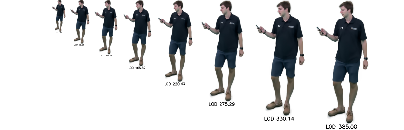
(a) Dataset A LODs shown at various scales

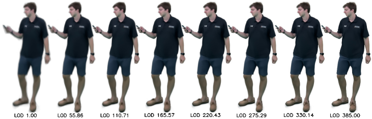
(b) Dataset A LODs shown at the same scale

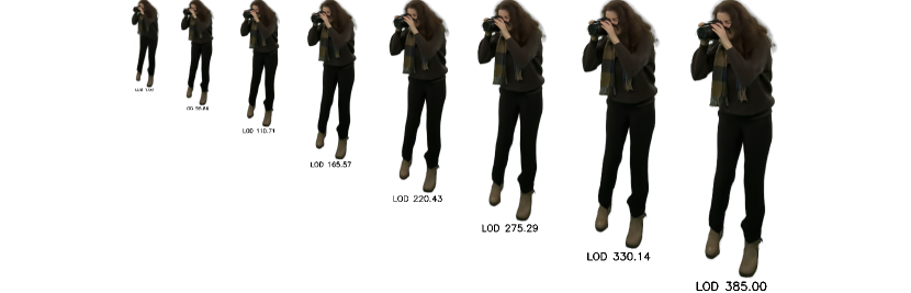
(c) Dataset C LODs shown at various scales

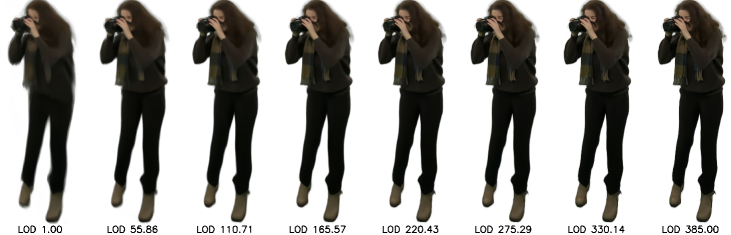
(d) Dataset C LODs shown at the same scale

Figure 1: Qualitative results rendering our continuous LFNs at multiple levels of detail for two datasets.

2.1 Comparision to NeRF

Neural radiance fields use volume rendering and 3D scene coordinates which provide 3D scene structure and multi-view consistency at the cost of requiring dozens to hundreds of evaluations per ray. Two continuous LOD methods for NeRFs are Mip-NeRF [Barron et al.(2021)Barron, Mildenhall, Tancik, Hedman, Martin-Brualla, and Srinivasan] and Zip-NeRF [Barron et al.(2023)Barron, Mildenhall, Verbin, Srinivasan, and Hedman]. Mip-NeRF uses integrated positional encoding to approximate a canonical frustum around a ray while Zip-NeRF uses multisampling of feature grid. Both of these methods are targeted solely toward anti-aliasing and flicker reduction rather than towards resource adaptivity. Hence, the entire model must be downloaded for rendering and the performance per pixel is the same at each scale. Furthermore, neither method is directly applicable to light field networks which rely on the spectral bias of ReLU MLPs and thus are incompatible with positional encoding and feature grids.

For reference purposes, we present quantitative results using Mip-NeRF [Barron et al.(2021)Barron, Mildenhall, Tancik, Hedman, Martin-Brualla, and Srinivasan] to display our datasets in Table 2. We train Mip-NeRF for $1$ million iterations with a batch size of $1024$ rays with the same $67\%$ foreground and $33\%$ background split in each batch. We also use the same training and test split for each dataset as in our experiments.

Table 2: Average Rendering Quality Comparison

Model	1/8	1/4	1/2	1/1
Continuous LOD LFN	28.06	29.79	28.44	27.40
Mip-NeRF	24.81	24.95	24.35	23.86

(a) PSNR (dB) at 1/8, 1/4, 1/2, and 1/1 scale.

Model	1/8	1/4	1/2	1/1
Continuous LOD LFN	0.8380	0.8751	0.8487	0.8455
Mip-NeRF	0.6819	0.6735	0.6451	0.6374

(b) SSIM at 1/8, 1/4, 1/2, and 1/1 scale.

Figure 2: Mip-NeRF rendering.

In our experiments, we observe that with our sampling scheme, Mip-NeRF is not able to separate the foreground and background cleanly as shown in Figure 2 which leads to worse PSNR and SSIM results.

In general, NeRF-based methods are better able to perform view-synthesis with high-frequency details due to their use of positional encoding and their 3D structure. MLP-based methods such as Mip-NeRF typically have a compact size ($\leq 10$ MB) but suffer from slow rendering times on the order of tens of seconds per image. Feature-grid NeRFs such as Instant-NGP [Müller et al.(2022)Müller, Evans, Schied, and Keller], Plenoxels [Yu et al.(2021)Yu, Fridovich-Keil, Tancik, Chen, Recht, and Kanazawa], and Zip-NeRF [Barron et al.(2023)Barron, Mildenhall, Verbin, Srinivasan, and Hedman] can achieve real-time rendering but at the cost of larger model sizes ($\geq 30$ MB). Factorized feature grids such as TensorRF [Chen et al.(2022)Chen, Xu, Geiger, Yu, and Su] promise both fast rendering and small model sizes. Note that the goal of our paper is to enable more granularity with continuous levels of detail for rendering and streaming purposes rather than improving view-synthesis quality.

References

- [Barron et al.(2021)Barron, Mildenhall, Tancik, Hedman, Martin-Brualla, and Srinivasan] Jonathan T. Barron, Ben Mildenhall, Matthew Tancik, Peter Hedman, Ricardo Martin-Brualla, and Pratul P. Srinivasan. Mip-NeRF: A multiscale representation for anti-aliasing neural radiance fields, 2021.
- [Barron et al.(2023)Barron, Mildenhall, Verbin, Srinivasan, and Hedman] Jonathan T. Barron, Ben Mildenhall, Dor Verbin, Pratul P. Srinivasan, and Peter Hedman. Zip-NeRF: Anti-aliased grid-based neural radiance fields. ICCV, 2023.
- [Chen et al.(2022)Chen, Xu, Geiger, Yu, and Su] Anpei Chen, Zexiang Xu, Andreas Geiger, Jingyi Yu, and Hao Su. TensoRF: Tensorial radiance fields. In European Conference on Computer Vision (ECCV), 2022.
- [Müller et al.(2022)Müller, Evans, Schied, and Keller] Thomas Müller, Alex Evans, Christoph Schied, and Alexander Keller. Instant neural graphics primitives with a multiresolution hash encoding. ACM Trans. Graph., 41(4), jul 2022. ISSN 0730-0301. 10.1145/3528223.3530127. URL https://doi.org/10.1145/3528223.3530127.
- [Yu et al.(2021)Yu, Fridovich-Keil, Tancik, Chen, Recht, and Kanazawa] Alex Yu, Sara Fridovich-Keil, Matthew Tancik, Qinhong Chen, Benjamin Recht, and Angjoo Kanazawa. Plenoxels: Radiance fields without neural networks, 2021.