Output-Feedback Nonlinear Model Predictive Control
with Iterative State- and Control-Dependent Coefficients

Abstract

By optimizing the predicted performance over a receding horizon, model predictive control (MPC) provides the ability to enforce state and control constraints. The present paper considers an extension of MPC for nonlinear systems that can be written in pseudo-linear form with state- and control-dependent coefficients. The main innovation is to apply quadratic programming iteratively over the horizon, where the predicted state trajectory is updated based on the updated control sequence. Output-feedback control is facilitated by using the block-observable canonical form for linear, time-varying dynamics. This control technique is illustrated on various numerical examples, including the Kapitza pendulum with slider-crank actuation, the nonholonomic integrator, the electromagnetically controlled oscillator, and the triple integrator with control-magnitude saturation.

I Introduction

By performing optimization over a future horizon, model predictive control (MPC) provides the means for controlling linear and nonlinear systems with state and control constraints [1, 2, 3, 4]. For systems with nonlinear dynamics, linearized plant models can be used iteratively to perform the receding-horizon optimization [5, 6]. Although convergence is not guaranteed, application of these techniques shows that they are effective in practice [7].

The present paper develops a novel approach to MPC for nonlinear systems by performing the iterative receding-horizon optimization based on state- and control-dependent coefficients. By recasting the nonlinear dynamics as pseudo-linear dynamics, state- and control-dependent coefficients (SCDCs) provide a heuristic technique for nonlinear control. Although guarantees are limited to local stabilization [8], SCDCs have seen widespread usage in diverse applications [9, 10, 11, 12, 13, 14, 15].

In the prior literature, SCDCs have been used within the context of MPC for nonlinear systems. In [16], a discrete-time SDRE technique is used with receding-horizon optimization based on the backward-propagating Riccati equation (BPRE) for enforcing state constraints. A related technique that fixes the current state over the future horizon is applied to quadcopter dynamics in [17].

In the present paper, we describe iterative state- and control-dependent MPC (ISCD-MPC) for output-feedback control of nonlinear systems. In order to assess the performance of this technique, we consider several well-studied benchmark problems, namely, the Kapitza pendulum [18, 19, 20], the nonholonomic integrator [21, 22, 23, 24, 25, 26, 27], the electromagnetically controlled oscillator [28, 29, 30], and the chain of integrators [31, 32]. The first three examples assume full-state feedback. For output-feedback control of the chain of integrators, we show how the state of the block-observable canonical form (BOCF) realization of the linear time-varying (LTV) pseudo-linear dynamics is an explicit function of the state and input matrices [33]. In effect, BOCF provides a deadbeat observer for the LTV pseudo-linear dynamics.

As in all nonlinear control techniques, especially those based on heuristics, a fundamental challenge is to demonstrate acceptable performance over the largest possible domain of attraction. For the chain of integrators, we thus investigate the convergence of the state trajectory over a grid of initial conditions for various values of the horizon.

II Notation

The symmetric matrix $P\in{\mathbb{R}}^{n\times n}$ is positive semidefinite (resp., positive definite) if all of its eigenvalues are nonnegative (resp., positive). Let $x_{(i)}$ denote the $i$th component of $x\in{\mathbb{R}}^{n}.$

III Problem Formulation

Consider the discrete-time nonlinear system

$$x_{k+1}=f(x_{k},u_{k}),$$ (1)

where, for all $k\geq 0$, $x_{k}\in{\mathbb{R}}^{n}$ is the state at step $k$, $x_{0}\in{\mathbb{R}}^{n}$ is the fixed initial condition, $u_{k}\in{\mathbb{R}}^{m}$ is the control input applied at step $k$, $u_{0}\in{\mathbb{R}}^{m}$ is the given initial control input, and $f\colon{\mathbb{R}}^{n}\times{\mathbb{R}}^{m}\to{\mathbb{R}}^{n}.$ Let $\ell\geq 2$ be the horizon length, and, for all $j\in\{1,\ldots,\ell\}$, let $x_{k,j}$ be the computed state for step $k+j$ obtained at step $k$ using

$$x_{k,j+1}=f(x_{k,j},u_{k,j}),$$ (2)

where $x_{k,0}\triangleq x_{k}$, $u_{k,0}\triangleq u_{k}$, and, for all $j\in\{1,\ldots,\ell-1\}$, $u_{k,j}$ is the computed control for step $k+j$ obtained at step $k.$ Note that

$$x_{k,1}=f(x_{k},u_{k}).$$ (3)

Next, for all $k\geq 0,$ consider the performance measure

$$J_{k} (u_{k,1},\ldots,u_{k,\ell-1})=\tfrac{1}{2}x_{k,\ell}^{\rm T}Q_{k,\ell}x_{k,\ell}$$

$$\quad+\tfrac{1}{2}\sum_{j=1}^{\ell-1}(x_{k,j}^{\rm T}Q_{k,j}x_{k,j}+u_{k,j}^{\rm T}R_{k,j}u_{k,j}),$$ (4)

where $Q_{k,\ell}\in{\mathbb{R}}^{n\times n}$ is the positive-semidefinite terminal weighting, and, for all $j\in\{1,\ldots,\ell-1\},$ $Q_{k,j}\in{\mathbb{R}}^{n\times n}$ is the positive-semidefinite state weighting, and $R_{k,j}\in{\mathbb{R}}^{m\times m}$ is the positive-definite control weighting.

At each time step $k\geq 0$, the objective is to find a sequence of control inputs $u_{k,1},\ldots,u_{k,\ell-1}$ such that $J_{k}$ is minimized subject to (2), (3), and the constraints

$${\mathcal{A}}v_{k}\leq b,$$ (5)

$${\mathcal{A}}_{\rm eq}v_{k}=b_{\rm eq},$$ (6)

$$\underline{v}_{s}\leq v_{k(s)}\leq\overline{v}_{s},~{}~{}~{}~{}~{}s\in\{1,\ldots,\ell(n+m)-m\},$$ (7)

where, ${\mathcal{A}},{\mathcal{A}}_{\rm eq}\in{\mathbb{R}}^{n_{\rm c}\times(\ell(n+m)-m)}$, $b,b_{\rm eq}\in{\mathbb{R}}^{n_{\rm c}}$, $n_{\rm c}\geq 0$ is the number of constraints, for all $k\geq 0$, $v_{k}\in{\mathbb{R}}^{\ell(n+m)-m}$ is defined by

$$v_{k}\triangleq\begin{bmatrix}x_{k,1}^{\rm T}&\cdots&x_{k,\ell}^{\rm T}&u_{k,1}^{\rm T}&\cdots&u_{k,\ell-1}^{\rm T}\end{bmatrix}^{\rm T},$$ (8)

and, for all $s\in\{1,\ldots,\ell(n+m)-m\},$ $\underline{v}_{s},\overline{v}_{s}\in{\mathbb{R}}$ are such that $\underline{v}_{s}<\overline{v}_{s}.$ In accordance with receding-horizon control, the first element $u_{k,1}$ of the sequence of computed controls is then applied to the system at time step $k+1$, that is, for all $k\geq 0,$

$$u_{k+1}=u_{k,1},$$ (9)

and $u_{k,2},\ldots,u_{k,\ell-1}$ are discarded. The optimization is performed beginning at step $k$ and is assumed to be completed before step $k+1.$ The optimization of (4) is performed by the iterative procedure detailed in the next section.

IV Iterative State- and Control-Dependent Model Predictive Control (ISCD-MPC)

We use a reformulation of the nonlinear system (1), namely, state- and control-dependent coefficients (SCDC) to present an iterative algorithm based on QP for computing $u_{k+1}$.

Let $\rho\geq 1$ denote the number of iterations, and let $i\in\{1,\ldots,\rho\}$ denote the index of the $i$th iteration at step $k.$ For all $k\geq 0$ and all $j\in\{1,\ldots,\ell\}$, let $x_{k,j|i}\in{\mathbb{R}}^{n}$ denote the computed state for step $k+j$ obtained at time step $k$ and iteration $i$. Similarly, let $u_{k,j|i}\in{\mathbb{R}}^{m}$ denote the computed control for step $k+j$ obtained at time step $k$ and iteration $i$.

Let $A\colon{\mathbb{R}}^{n}\times{\mathbb{R}}^{m}\to{\mathbb{R}}^{n\times n}$ and $B\colon{\mathbb{R}}^{n}\times{\mathbb{R}}^{m}\to{\mathbb{R}}^{n\times m}$ be such that, for all $x\in{\mathbb{R}}^{n}$ and all $u\in{\mathbb{R}}^{m},$

$$f(x,u)=A(x,u)x+B(x,u)u,$$ (10)

which is an SCDC representation. For all $j\in\{1,\ldots,\ell\}$, the computed state $x_{k,j|i}$ is obtained using

$$x_{k,j+1|i}=A_{k,j|i}x_{k,j|i}+B_{k,j|i}u_{k,j|i},$$ (11)

where

$$A_{k,j|i}\triangleq A(x_{k,j|i},u_{k,j|i}),\quad B_{k,j|i}\triangleq B(x_{k,j|i},u_{k,j|i}),$$ (12)

and

$$x_{k,0|i} \triangleq x_{k},$$ (13)

$$u_{k,0|i} \triangleq u_{k}.$$ (14)

Note that (10)–(14) implies that

$$x_{k,1|i} =f(x_{k},u_{k})$$ (15)

$$=A(x_{k},u_{k})x_{k}+B(x_{k},u_{k})u_{k}$$ (16)

$$=A_{k,0|i}x_{k}+B_{k,0|i}u_{k}.$$ (17)

Now, we use iterations of QP to compute $u_{k,j|i}$. For all $k\geq 0$ and all $j\in\{1,\ldots,\ell-1\},$ initialize

$$u_{k,j|1}\triangleq u_{k}.$$ (18)

For all $i\in\{2,\ldots,\rho\}$, let the computed control sequence $\{u_{k,1|i},\ldots,u_{k,\ell-1|i}\}$ be the solution of the quadratic program

$$\min_{\mu_{1},\ldots,\mu_{\ell-1}}\Bigg{(}\tfrac{1}{2}\xi_{\ell}^{\rm T}Q_{k,\ell}\xi_{\ell}+\tfrac{1}{2} \sum_{j=1}^{\ell-1}(\xi_{j}^{\rm T}Q_{k,j}\xi_{j}+\mu_{j}^{\rm T}R_{k,j}\mu_{j})\Bigg{)},$$ (19)

subject to:   

$$\xi_{1}=x_{k,1|i},$$ (20)

$$\xi_{j+1}=A_{k,j|i-1}\xi_{j}+B_{k,j|i-1}\mu_{j},$$ (21)

$${\mathcal{A}}\nu\leq b,$$ (22)

$${\mathcal{A}}_{\rm eq}\nu=b_{\rm eq},$$ (23)

$$\underline{v}_{s}\leq\nu_{(s)}\leq\overline{v}_{s},~{}~{}~{}~{}~{}s\in\{1,\ldots,\ell(n+m)-m\},$$ (24)

where $\nu\in{\mathbb{R}}^{\ell(n+m)-m}$ is defined by

$$\nu\triangleq\begin{bmatrix}\xi_{1}^{\rm T}&\cdots&\xi_{\ell}^{\rm T}&\mu_{1}^{\rm T}&\cdots&\mu_{\ell-1}^{\rm T}\end{bmatrix}^{\rm T}.$$ (25)

Finally, let

$$u_{k+1}=u_{k,1|\rho}.$$ (26)

V Stopping Criterion and Warm Starting

We present a modification of ISCD-MPC that can reduce the computational burden of the algorithm. In particular, at each step $k\geq 0$, the modification uses a stopping criterion to potentially stop the iterations before reaching iteration $\rho$. Moreover, the modification uses the control sequence obtained at the last iteration of step $k$ to form the control sequence for the first iteration of step $k+1.$

Let $\varepsilon>0$ be a tolerance used as the stopping criterion. For all $k\geq 0$ and all $i\in\{1,\ldots,\rho\},$ define

$$U_{k|i}\triangleq\begin{bmatrix}u_{k,1|i}^{\rm T}&\cdots&u_{k,\ell-1|i}^{\rm T}\end{bmatrix}^{\rm T}\in{\mathbb{R}}^{m(\ell-1)}.$$ (27)

For each $k\geq 0,$ define $\rho_{k}\in\{2,\ldots,\rho\}$ by

$$\rho_{k}\triangleq\min\{\rho,\min\{i\in\{2,\ldots,\rho\}\colon\|U_{k|i}-U_{k|i-1}\|<\varepsilon\}\},$$ (28)

and let $\rho_{k}$ be the index of the last iteration. For all $j\in\{1,\ldots,\ell-1\},$ initialize

$$u_{0,j|1}\triangleq u_{0},$$ (29)

and, for all $k\geq 1$ and all $j\in\{1,\ldots,\ell-1\},$ initialize

$$u_{k,j|1} \triangleq\begin{cases}u_{k-1,j+1|\rho_{k-1}},&j\in\{1,\ldots,\ell-2\},\\ u_{k-1,\ell-1|\rho_{k-1}},&j=\ell-1.\end{cases}$$ (30)

For all examples in this paper, we use ISCD-MPC with the stopping criteria defined by (27) and (28), and the warm starting defined by (29) and (30).

Each example in this paper includes magnitude saturation of the control input. This constraint can be enforced directly using QP. In the present paper, however, we represent the magnitude saturation $\sigma(u)$ as $[\sigma(u)/u]u,$ so that $B\sigma(u)/u$ is treated as a control-dependent coefficient. Numerical experience shows that this technique is more reliable than direct enforcement of control constraints using QP.

The input nonlinearity $\sigma$ has the property that $\sigma(u)/u$ has a removable singularity at $u=0$ with the value $\sigma(0)/0\triangleq\lim_{u\to 0}\sigma(u)/u.$ Similarly, $\sin(0)/0\triangleq 1.$

All examples in this paper are performed using a sampled-data control setting. In particular, MATLAB ‘ode45’ command is used to simulate the continuous-time, nonlinear dynamics, where the ‘ode45’ relative and absolute tolerances are set to $10^{-5}.$ In addition, for all examples, we use MATLAB ‘quadprog’ command to perform QP, where we choose $Q_{k,j}$ and $R_{k,j}$ to be independent of $k$ and $j$, and we thus write $Q$ and $R$.

Example 1.

Kapitza pendulum with slider-crank actuation subject to control-magnitude saturation. Consider the Kapitza pendulum shown in Figure 1, where the control input $u$ is the angular wheel speed. Assuming for simplicity that $(\sin\phi)^{2}\ll(a/r)^{2},$ the equations of motion are given by

$$\ddot{\theta}-\frac{g}{l}\sin\theta+\frac{r}{l}\left(\cos\phi+\frac{r\cos 2\phi}{a}\right)(\sin\theta)\left(\sigma(u)\right)^{2}=0,$$ (31)

$$\dot{\phi}=\sigma(u),$$ (32)

where $r$ is the radius of the wheel, $a$ is the length of the arm, $l$ is the length of the pendulum, $g$ is the acceleration of gravity, and $\sigma\colon{\mathbb{R}}\to{\mathbb{R}}$ is the control-magnitude saturation function defined by

$$\sigma(u)\triangleq\begin{cases}u_{\max},&u>u_{\max},\\ u,&u_{\min}\leq u\leq u_{\max},\\ u_{\min},&u<u_{\min},\end{cases}$$ (33)

and $u_{\min},u_{\max}\in{\mathbb{R}}$ are the lower and upper magnitude saturation levels.

Figure 1: Example 1. Kapitza pendulum with slider-crank actuation. The base of the pendulum, which is confined to a vertical slot, is actuated by an arm of length $a$ attached to the circumference of the wheel of radius $r.$

Let $x\triangleq\begin{bmatrix}\theta&\dot{\theta}&\phi\end{bmatrix}^{\rm T}$ be the state, and it follows from (31) and (32) that

$$\dot{x} =\begin{bmatrix}x_{(2)}\\ \frac{g}{l}\sin x_{(1)}\\ 0\end{bmatrix}$$

$$\quad+\begin{bmatrix}0\\ -\frac{r}{l}\left(\cos x_{(3)}+\frac{r\cos 2x_{(3)}}{a}\right)(\sin x_{(1)})(\sigma(u))^{2}\\ \sigma(u)\end{bmatrix}.$$ (34)

For all $k\geq 0$ and all $t\in[kT_{\rm s},(k+1)T_{\rm s})$, we consider $u(t)=u_{k},$ where $u_{k}\in{\mathbb{R}}$ is the discrete-time control determined by the algorithm. Using Euler integration, the discrete-time approximation of (34) is given by

$$x_{k+1}=x_{k}+T_{\rm s}\begin{bmatrix}x_{k{(2)}}\\ \frac{g}{l}\sin x_{k{(1)}}\\ 0\end{bmatrix}$$

$$+T_{\rm s}\begin{bmatrix}0\\ -\frac{r}{l}\left(\cos x_{k{(3)}}+\frac{r\cos 2x_{k{(3)}}}{a}\right)(\sin x_{k{(1)}})(\sigma(u_{k}))^{2}\\ \sigma(u_{k})\end{bmatrix},$$ (35)

where, for all $k\geq 0,$ $x_{k}\triangleq x(kT_{\rm s})$. To implement ISCD-MPC, we consider the SCDC representation of (35) given by

$$x_{k+1} =x_{k}+T_{\rm s}\begin{bmatrix}0&1&0\\ \frac{g\sin x_{k{(1)}}}{lx_{k{(1)}}}&0&0\\ 0&0&0\end{bmatrix}x_{k}$$

$$\quad+T_{\rm s}\begin{bmatrix}0\\ \frac{-\frac{r}{l}\left(\cos x_{k(3)}+\frac{r\cos 2x_{k(3)}}{a}\right)(\sin x_{k(1)})(\sigma(u_{k}))^{2}}{u_{k}}\\[4.30554pt] \frac{\sigma(u_{k})}{u_{k}}\end{bmatrix}u_{k}.$$ (36)

Figure 2 shows $x$ and $\sigma(u)$ using ISCD-MPC, where

$$T_{\rm s}=0.1\,{\rm s},\quad l=0.25\,{\rm m},\quad r=1\,{\rm m},$$ (37)

$$a=2\,{\rm m},\quad g=9.81\,\tfrac{{\rm m}}{{\rm s}^{2}},$$ (38)

$$x_{0}=\begin{bmatrix}\pi\,{\rm rad}&\pi\,\tfrac{\rm rad}{{\rm s}}&\pi\,{\rm rad}\end{bmatrix}^{\rm T},\quad u_{0}=0,$$ (39)

$$u_{\max}=-u_{\min}=3\,\tfrac{\rm rad}{{\rm s}},\quad\ell=50,\quad\rho=30,$$ (40)

$$\varepsilon=10^{-3},\quad Q={\rm diag}(10^{4},10^{3},10^{6}),\quad R=1.\penalty 9999\hbox{}\nobreak\hfill\quad\hbox{$\diamond$}$$ (41)

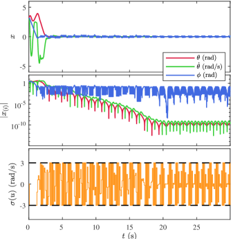
Figure 2: Example 1. Stabilization of Kapitza pendulum with slider-crank actuation subject to control-magnitude saturation.

Example 2.

Nonholonomic integrator with control-magnitude saturation. Consider the continuous-time nonholonomic integrator with control-magnitude saturation given by

$$\dot{x}=\begin{bmatrix}1&0\\ 0&1\\ -x_{(2)}&x_{(1)}\end{bmatrix}\sigma(u),$$ (42)

where $\sigma\colon{\mathbb{R}}^{2}\to{\mathbb{R}}^{2}$ is the control-magnitude saturation function

$$\sigma(u)\triangleq\begin{bmatrix}\bar{\sigma}(u_{(1)})\\ \bar{\sigma}(u_{(2)})\end{bmatrix},$$ (43)

where $\bar{\sigma}\colon{\mathbb{R}}\to{\mathbb{R}}$ is defined by

$$\bar{\sigma}(u)\triangleq\begin{cases}u_{\max},&u>u_{\max},\\ u,&u_{\min}\leq u\leq u_{\max},\\ u_{\min},&u<u_{\min},\end{cases}$$ (44)

and $u_{\min},u_{\max}\in{\mathbb{R}}$ are the lower and upper magnitude saturation levels, respectively. Let $T_{\rm s}>0$, and, for all $k\geq 0$ and all $t\in[kT_{\rm s},(k+1)T_{\rm s})$, consider $u(t)=u_{k},$ where $u_{k}\in{\mathbb{R}}$ is the discrete-time control determined by the algorithm. Using Euler integration, the discrete-time approximation of (34) is given by

$$x_{k+1}=x_{k}+T_{\rm s}\begin{bmatrix}1&0\\ 0&1\\ -x_{k{(2)}}&x_{k{(1)}}\end{bmatrix}\sigma(u_{k}),$$ (45)

where, for all $k\geq 0,$ $x_{k}\triangleq x(kT_{\rm s})$. To implement ISCD-MPC with control magnitude saturation, we consider the SCDC representation of (45) given by

$$x_{k+1}=x_{k}+B(x_{k},u_{k})u_{k},$$ (46)

where

$$B(x_{k},u_{k})=T_{\rm s}\begin{bmatrix}1&0\\ 0&1\\ -x_{k{(2)}}&x_{k{(1)}}\end{bmatrix}\cdot\begin{cases}I_{2},&{\sigma(u_{k})=u_{k}},\\ \frac{\sigma(u_{k})u_{k}^{\rm T}}{\|u_{k}\|^{2}},&{\sigma(u_{k})\neq u_{k}}.\end{cases}$$ (47)

Figure 3 shows $x$ and $\sigma(u)$ using ISCD-MPC, where

$$T_{\rm s}=0.01\,{\rm s},\quad x_{0}=\begin{bmatrix}10&10&10\end{bmatrix}^{\rm T},$$ (48)

$$u_{0}=0,\quad u_{\max}=-u_{\min}=1,\quad\ell=500,\quad\rho=50,$$ (49)

$$\varepsilon=10^{-3},\quad Q={\rm diag}(10^{3},10^{3},10^{4}),\quad R=I_{2}.\penalty 9999\hbox{}\nobreak\hfill\quad\hbox{$\diamond$}$$ (50)

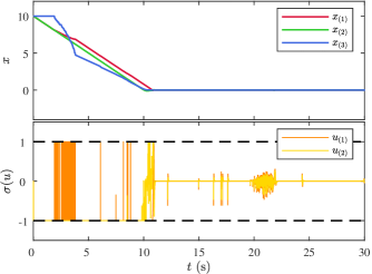
Figure 3: Example 2. Stabilization of the nonholonomic integrator subject to control-magnitude saturation.

Example 3.

Electromagnetically controlled oscillator. Consider the electromagnetically controlled oscillator shown in Figure 4, where $q$ is the position of the mass $\bar{m}$, $\bar{k}$ is the stiffness of the spring, $\bar{b}$ is damping, $\bar{q}$ is the distance from mass to the magnet when the spring is relaxed, and $\bar{i}$ is the current. Define $z\triangleq\begin{bmatrix}q&\dot{q}\end{bmatrix}^{\rm T}$. Then, the governing dynamics of the electromagnetically controlled oscillator are given by

$$\dot{z}=\begin{bmatrix}z_{(2)}\\ -\frac{\bar{b}}{\bar{m}}z_{(2)}-\frac{\bar{k}}{\bar{m}}z_{(1)}+\frac{\bar{\varepsilon}(\sigma(\bar{i}))^{2}}{m(\bar{q}-z_{(1)})^{2}}\end{bmatrix},$$ (51)

where $\bar{\varepsilon}$ is a force constant representing the strength of the electromagnet, and $\sigma\colon{\mathbb{R}}\to{\mathbb{R}}$ is the control-magnitude saturation function defined by (33).

Figure 4: Electromagnetically controlled oscillator

Let $r\in(0,\bar{q})$ be the desired position of the mass, and define $x\triangleq z-\begin{bmatrix}r&0\end{bmatrix}^{\rm T},$ which implies $\dot{x}=\dot{z}.$ It thus follows from (51) that

$$\dot{x}=\begin{bmatrix}x_{(2)}\\ -\frac{\bar{b}}{\bar{m}}x_{(2)}-\frac{\bar{k}}{\bar{m}}(x_{(1)}+r)+\frac{\bar{\varepsilon}(\sigma(\bar{i}))^{2}}{\bar{m}(\bar{q}-x_{(1)}-r)^{2}}\end{bmatrix}.$$ (52)

Let $T_{\rm s}>0$, and, for all $k\geq 0$ and all $t\in[kT_{\rm s},(k+1)T_{\rm s})$, consider $\bar{i}(t)=\bar{i}_{k},$ where $\bar{i}_{k}\in{\mathbb{R}}$ is the discrete-time current determined by the algorithm. Using Euler integration, the discrete-time approximation of (52) is given by

$$x_{k+1} =x_{k}+T_{\rm s}\begin{bmatrix}x_{k{(2)}}\\ -\frac{\bar{b}x_{k{(2)}}}{\bar{m}}-\frac{\bar{k}x_{k{(1)}}}{\bar{m}}+\frac{\bar{\varepsilon}(\sigma(\bar{i}_{k}))^{2}}{\bar{m}(\bar{q}-x_{k{(1)}}-r)^{2}}-\frac{kr}{m}\end{bmatrix}$$

$$=x_{k}+T_{\rm s}\begin{bmatrix}x_{k{(2)}}\\ -\frac{\bar{b}x_{k{(2)}}}{\bar{m}}-\frac{\bar{k}x_{k{(1)}}}{\bar{m}}+\frac{\bar{\varepsilon}(\sigma_{{\rm a}}(u_{k}))^{2}}{\bar{m}(\bar{q}-x_{k{(1)}}-r)^{2}}\end{bmatrix},$$ (53)

where, for all $k\geq 0,$ $x_{k}\triangleq x(kT_{\rm s})$,

$$u_{k}\triangleq\bar{i}_{k}-\bar{i}_{*},$$ (54)

where $\bar{i}_{*}\triangleq\sqrt{\frac{(\bar{q}-r)^{2}\bar{k}r}{\bar{\varepsilon}}}$ is the equilibrium current, and $\sigma_{\rm a}\colon{\mathbb{R}}\to{\mathbb{R}}$ is the asymmetric control-magnitude saturation function defined by

$$\sigma_{\rm a}(u)\triangleq\begin{cases}u_{\max}-\bar{i}_{*},&u>u_{\max}-\bar{i}_{*},\\ u,&u_{\min}-\bar{i}_{*}\leq u\leq u_{\max}-\bar{i}_{*},\\ u_{\min}-\bar{i}_{*},&u<u_{\min}-\bar{i}_{*}.\end{cases}$$ (55)

To implement ISCD-MPC with control magnitude saturation, we consider the SCDC representation of (53) given by

$$x_{k+1} =x_{k}+T_{\rm s}\begin{bmatrix}0&1\\ -\frac{\bar{k}}{\bar{m}}&-\frac{\bar{b}}{\bar{m}}\end{bmatrix}x_{k}$$

$$\quad+T_{\rm s}\begin{bmatrix}0\\ \frac{\bar{\varepsilon}(\sigma_{\rm a}(u_{k}))^{2}}{\bar{m}u_{k}(\bar{q}-x_{k{(1)}}-r)^{2}}\end{bmatrix}u_{k}.$$ (56)

Figure 5 shows $z$ and $\sigma(\bar{i})$ using ISCD-MPC, where

$$T_{\rm s}=0.01\,{\rm s},\quad z(0)=\begin{bmatrix}0{\,\rm m}&0{\,\rm m/s}\end{bmatrix}^{\rm T},$$ (57)

$$r=2{\,\rm m},\quad\bar{q}=3{\,\rm m},\quad\bar{\varepsilon}=1{\,\rm N.m^{2}.A^{-2}}$$ (58)

$$\bar{k}=5{\,\rm N/m},\quad\bar{m}=1{\,\rm kg},\quad\bar{c}=5{\,\rm N.s/m},$$ (59)

$$u_{0}=10^{-2}{\,\rm A},\quad u_{\max}=-u_{\min}=10{\,\rm A},$$ (60)

$$\ell=300,\quad\rho=50,\quad\varepsilon=10^{-3},$$ (61)

$$Q={\rm diag}(10^{3},10^{2}),\quad R=1.$$ (62)

Note that the current $\bar{i}$ converges to $\bar{i}_{*}=\sqrt{10}$ A.  $\diamond$

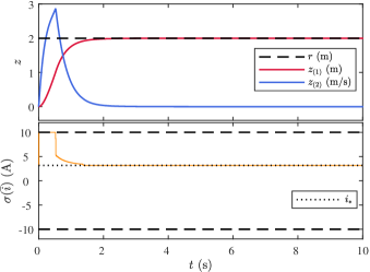
Figure 5: Example 3. Command following for the electromagnetically controlled oscillator subject to control-magnitude saturation.

VI Output-Feedback Control of Input-Output Systems

Consider the discrete-time input-output system

$$y_{k} =-\sum_{\tau=1}^{n}f_{\tau}(y_{k-1},\ldots,y_{k-n},u_{k-1},\ldots,u_{k-n})y_{k-\tau}$$

$$\quad+\sum_{\tau=1}^{n}g_{\tau}(y_{k-1},\ldots,y_{k-n},u_{k-1},\ldots,u_{k-n})u_{k-\tau},$$ (63)

where, for all $\tau\in\{1,\ldots,n\}$, $f_{\tau}\colon{\mathbb{R}}^{p}\times\cdots\times{\mathbb{R}}^{p}\times{\mathbb{R}}^{m}\times\cdots\times{\mathbb{R}}^{m}\to{\mathbb{R}}^{p\times p}$ and $g_{\tau}\colon{\mathbb{R}}^{p}\times\cdots\times{\mathbb{R}}^{p}\times{\mathbb{R}}^{m}\times\cdots\times{\mathbb{R}}^{m}\to{\mathbb{R}}^{p\times m},$ and, for all $k\geq 0,$ $y_{k}\in{\mathbb{R}}^{p}$ is the measured output, $u_{k}\in{\mathbb{R}}^{m}$ is the control input, and

$$y_{-1}=\cdots=y_{-n}=0,$$ (64)

$$u_{-1}=\cdots=u_{-n}=0.$$ (65)

For all $\tau\in\{1,\ldots,n\}$ and all $k\geq 0$, define

$$F_{\tau,k} \triangleq f_{\tau}(y_{k-1},\ldots,y_{k-n},u_{k-1},\ldots,u_{k-n})\in{\mathbb{R}}^{p\times p},$$ (66)

$$G_{\tau,k} \triangleq g_{\tau}(y_{k-1},\ldots,y_{k-n},u_{k-1},\ldots,u_{k-n})\in{\mathbb{R}}^{p\times m}.$$ (67)

Then, for all $k\geq 0$, the block observable canonical form (BOCF) of (63) is given by [34]

$$x_{k+1} =A(x_{k},u_{k})x_{k}+B(x_{k},u_{k})u_{k},$$ (68)

$$y_{k} =Cx_{k},$$ (69)

where

$$A(x_{k},u_{k})\triangleq\begin{bmatrix}-F_{1,k+1}&1&0&\cdots&0\\ -F_{2,k+1}&0&1&\cdots&0\\ \vdots&\vdots&\vdots&\ddots&\vdots\\ -F_{3,k+1}&0&0&\cdots&1\\ -F_{n,k+1}&0&0&\cdots&0\end{bmatrix}\in{\mathbb{R}}^{np\times np},$$ (70)

$$B(x_{k},u_{k})\triangleq\begin{bmatrix}G_{1,k+1}\\ G_{2,k+1}\\ \vdots\\ G_{n,k+1}\end{bmatrix}\in{\mathbb{R}}^{np\times m},$$ (71)

$$C\triangleq\begin{bmatrix}I_{p}&0&\cdots&0&0\end{bmatrix}\in{\mathbb{R}}^{p\times np},$$ (72)

and

$$x_{k}\triangleq\begin{bmatrix}x_{k(1)}\\ \vdots\\ x_{k(n)}\end{bmatrix}\in{\mathbb{R}}^{np},$$ (73)

where

$$x_{k(1)}\triangleq y_{k},$$ (74)

and, for all $\tau\in\{2,\ldots,n\},$ $x_{k(\tau)}\in{\mathbb{R}}^{p}$ is defined by

$$x_{k(\tau)}\triangleq\sum_{s=1}^{n-\tau+1}-F_{\tau+s-1,k}y_{k-s}+\sum_{s=1}^{n-\tau+1}G_{\tau+s-1,k}u_{k-s}.$$ (75)

Since (68) represents pseudo-linear dynamics of the nonlinear system (63) using SCDC, we can apply ISCD-MPC, as demonstrated in the following example.

Example 4.

Triple-integrator with asymmetric control-magnitude saturation. Consider the continuous-time system

$$\dot{x}(t) =\begin{bmatrix}0&1&0\\ 0&0&1\\ 0&0&0\end{bmatrix}x(t)+\begin{bmatrix}0\\ 0\\ 1\end{bmatrix}\sigma(u(t)),$$ (76)

$$y(t) =\begin{bmatrix}1&0&0\end{bmatrix}x,$$ (77)

where, for all $t\geq 0$, $x(t)\in{\mathbb{R}}^{3}$ is the state, $u(t)\in{\mathbb{R}}$ is the control input, $y(t)\in{\mathbb{R}}$ is the measured output, and $\sigma\colon{\mathbb{R}}\to{\mathbb{R}}$ is the control-magnitude saturation function defined by (33). If, for all $t\geq 0$, $u(t)\in[u_{\min},u_{\max}]$, then (76) and (77) yield the transfer function

$$G_{\rm c}(s)=\frac{1}{s^{3}},$$ (78)

which is a triple integrator. Let $T_{\rm s}=0.1$ s be the sample time, and, for all $k\geq 0$, define $y_{k}\triangleq y(kT_{\rm s})$. Moreover, for all $k\geq 0$ and all $t\in[kT_{\rm s},(k+1)T_{\rm s})$, let $u(t)=u_{k}$. The discrete-time counterpart of (78), which is the transfer function from $u_{k}$ to $y_{k}$, is given by

$$G({\bf q})=\frac{5({\bf q}^{2}+4{\bf q}+1)}{3\times 10^{4}({\bf q}-1)^{3}},$$ (79)

where ${\bf q}$ is the forward-shift operator. Note that the zeros of (79) are sampling zeros, and that $G$ is nonminimum phase [35]. Using (79), the discrete-time input-output counterpart of (76) and (77) is given by

$$y_{k} =3y_{k-1}-3y_{k-2}+y_{k-3}$$

$$\quad+\tfrac{5}{3\times 10^{4}}\big{(}\sigma(u_{k-1})+4\sigma(u_{k-2})+\sigma(u_{k-3})\big{)},$$ (80)

which has the form of (63), where

$$F_{1,k}=3,\quad F_{2,k}=-3,\quad F_{3,k}=1,$$ (81)

$$G_{1,k}=\tfrac{5\sigma(u_{k-1})}{3\times 10^{4}u_{k-1}},\quad G_{2,k}=\tfrac{20\sigma(u_{k-2})}{3\times 10^{4}u_{k-2}},$$ (82)

$$G_{3,k}=\tfrac{5\sigma(u_{k-3})}{3\times 10^{4}u_{k-3}}.$$ (83)

The red curves in Figure 6 shows $x$ and $\sigma(u)$ using ISCD-MPC, where

$$x(0)=\begin{bmatrix}300&0&0\end{bmatrix}^{\rm T},\quad\ell=200,\quad\rho=30,$$ (84)

$$\varepsilon=10^{-3},\quad Q=10^{10}I_{3},\quad R=1,$$ (85)

$$u_{\max}=2,\quad u_{\min}=-1.$$ (86)

Next, we compare the performance of ISCD-MPC and the nested-saturation controller of [31]. We consider the output-feedback version of [31] presented in [32]. Note that [31, 32] are not predictive, whereas ISCD-MPC is a predictive algorithm. The blue curves in Figure 6 shows $x$ and $\sigma(u)$ with the nested-saturation controller of [32], where

$$u_{0}=0,\quad\lambda_{1}=\lambda_{2}=\lambda_{3}=-0.1,$$ (87)

$$\overline{\varepsilon}_{1}=-\underline{\varepsilon}_{1}=0.24,\quad\overline{\varepsilon}_{2}=-\underline{\varepsilon}_{2}=0.25,$$ (88)

$$\underline{\varepsilon}_{2}=-0.51,\quad\overline{\varepsilon}_{3}=1.51.\penalty 9999\hbox{}\nobreak\hfill\quad\hbox{$\diamond$}$$ (89)

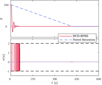
Figure 6: Example 4. Comparison of output-feedback stabilization of a triple integrator subject to asymmetric control-magnitude saturation using ISCD-MPC with the nested-saturation controller of [32].

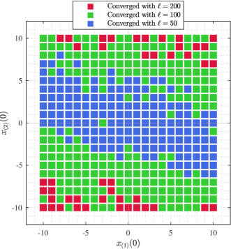
Figure 7: Example 5. Domain of attraction for the triple integrator (78) subject to asymmetric control-magnitude saturation, where the initial conditions are $x_{(1)}(0),x_{(2)}(0)\in[-10,10]$ and $x_{(3)}(0)=0.$ Note that the domain of attraction becomes larger as the horizon $\ell$ of ISCD-MPC increases.

Example 5.

Domain of attraction for a triple integrator with asymmetric control-magnitude saturation. For the chain of integrators in Example 4, we investigate the domain of attraction using ISCD-MPC. In particular, we consider the grid of initial conditions where $x_{(1)}(0),x_{(2)}(0)\in\{-10,9,\ldots,9,10\}$ and $x_{(3)}(0)=0.$ Each simulation is run for $60$ s, which, since $T_{\rm s}=0.1$ s, yields 600 step. The convergence criterion is $\sum_{k=580}^{600}\|x_{k}\|<0.01.$ Figure 7 shows the domain of attraction of ISCD-MPC for $\ell\in\{50,100,200\}$. Numerical simulations with larger values of $\ell$ (not shown) suggest that ISCD-MPC provides semiglobal stabilization.  $\diamond$

VII Conclusions

This paper presented ISCD-MPC, which is a model predictive control technique for full-state- or output-feedback control of nonlinear systems. In order to address the nonlinear dynamics, a state- and control-dependent parameterization of the nonlinearities was used. The nonlinearities were handled by means of an iterative technique involving QP. This technique was illustrated by means of a collection of nonlinear benchmark problems.

A fundamental requirement of this technique is the need for the state- and control-dependent iteration of QP to converge at each step. Numerically, this iteration was found to be extremely reliable, a property shared with the iLQR technique [6, 7]. A deeper understanding of the mechanisms responsible for convergence warrants further investigation.

Several extensions of ISCD-MPC can be considered. Further numerical studies are required to understand the relationship between the achievable domain of attraction and the required horizon length [36], as well as the choice of the control- and state-dependent coefficient. In particular, based on Example 5, we conjecture that, with sufficiently large horizon, ISCD-MPC semiglobally stabilizes chains of integrators of arbitrary length with arbitrary zeros.

References

- [1] S. S. Keerthi and E. G. Gilbert, “Optimal infinite-horizon feedback laws for a general class of constrained discrete-time systems: stability and moving horizon approximations,” J. Optim. Theory Appl., vol. 57, pp. 265–293, 1988.
- [2] W. Kwon and S. Han, Receding Horizon Control: Model Predictive Control for State Models. Springer, 2006.
- [3] E. F. Camacho and C. Bordons, Model Predictive Control, 2nd ed. Springer, 2007.
- [4] U. Eren, A. Prach, B. B. Koçer, S. V. Raković, E. Kayacan, and B. Açıkmeşe, “Model predictive control in aerospace systems: Current state and opportunities,” J. Guid. Contr. Dyn., vol. 40, no. 7, pp. 1541–1566, 2017.
- [5] W. Li and E. Todorov, “Iterative linear quadratic regulator design for nonlinear biological movement systems,” in ICINCO, 2004, pp. 222–229.
- [6] E. Todorov and W. Li, “A generalized iterative LQG method for locally-optimal feedback control of constrained nonlinear stochastic systems,” in Proc. Amer. Contr. Conf., 2005, pp. 300–306.
- [7] J. Chen, W. Zhan, and M. Tomizuka, “Constrained iterative LQR for on-road autonomous driving motion planning,” in IEEE Int. Conf. Intell. Trans. Sys., 2017, pp. 1–7.
- [8] D. A. Bristow, M. Tharayil, and A. G. Alleyne, “A survey of iterative learning control,” IEEE Contr. Sys. Mag., vol. 26, pp. 96–114, 2006.
- [9] R. Findeisen, L. Imsland, F. Allgower, and B. A. Foss, “State and output feedback nonlinear model predictive control: An overview,” Eur. J. Contr., vol. 9, no. 2-3, pp. 190–206, 2003.
- [10] C. P. Mracek and J. R. Cloutier, “Control designs for the nonlinear benchmark problem via the state-dependent riccati equation method,” Int. J. Robust Nonlin. Contr., vol. 8, no. 4-5, pp. 401–433, 1998.
- [11] E. B. Erdem and A. G. Alleyne, “Design of a class of nonlinear controllers via state dependent Riccati equations,” IEEE Trans. Contr. Sys. Tech., vol. 12, no. 1, pp. 133–137, 2004.
- [12] T. Çimen, “Systematic and effective design of nonlinear feedback controllers via the state-dependent Riccati equation (SDRE) method,” Ann. Rev. Contr., vol. 34, no. 1, pp. 32–51, 2010.
- [13] A. Weiss, I. Kolmanovsky, M. Baldwin, R. S. Erwin, and D. S. Bernstein, “Forward-integration Riccati-based feedback control for spacecraft rendezvous maneuvers on elliptic orbits,” in Proc. Conf. Dec. Contr., 2012, pp. 1752–1757.
- [14] A. Prach, O. Tekinalp, and D. S. Bernstein, “Output-feedback control of linear time-varying and nonlinear systems using the forward propagating Riccati equation,” J. Vib. Contr., vol. 24, no. 7, pp. 1239–1263, 2018.
- [15] P. Tsiotras, M. Corless, and M. Rotea, “Counterexample to a recent result on the stability of nonlinear systems,” IMA J. Math. Contr. Info., vol. 13, no. 2, pp. 129–130, 1996.
- [16] I. Chang and J. Bentsman, “Constrained discrete-time state-dependent Riccati equation technique: A model predictive control approach,” in Proc. Conf. Dec. Contr., 2013, pp. 5125–5130.
- [17] P. Ru and K. Subbarao, “Nonlinear model predictive control for unmanned aerial vehicles,” Aerospace, vol. 4, no. 2, p. 31, 2017.
- [18] J. M. Berg and I. M. Wickramasinghe, “Vibrational control without averaging,” Automatica, vol. 58, pp. 72 – 81, 2015.
- [19] Z. Artstein, “The pendulum under vibrations revisited,” Nonlinearity, vol. 34, pp. 394–410, 2021.
- [20] M. A. Ahrazoğlu, S. A. U. Islam, A. Goel, and D. S. Bernstein, “Vibrational stabilization of the Kapitza pendulum using model predictive control with constrained base displacement,” in Proc. Amer. Contr. Conf., 2023, pp. 2640–2645.
- [21] R. W. Brockett et al., “Asymptotic stability and feedback stabilization,” Differential Geometric Control Theory, vol. 27, no. 1, pp. 181–191, 1983.
- [22] A. Bloch, M. Reyhanoglu, and N. McClamroch, “Control and stabilization of nonholonomic dynamic systems,” IEEE Trans. Autom. Contr., vol. 37, no. 11, pp. 1746–1757, 1992.
- [23] R. M. Murray and S. S. Sastry, “Nonholonomic motion planning: Steering using sinusoids,” IEEE Trans. Autom. Contr., vol. 38, no. 5, pp. 700–716, 1993.
- [24] I. Kolmanovsky and N. H. McClamroch, “Developments in nonholonomic control problems,” IEEE Contr. Sys. Mag., vol. 15, no. 6, pp. 20–36, 1995.
- [25] A. Bloch and S. Drakunov, “Stabilization and tracking in the nonholonomic integrator via sliding modes,” Sys. Contr. Lett., vol. 29, no. 2, pp. 91–99, 1996.
- [26] J. P. Hespanha and A. S. Morse, “Stabilization of nonholonomic integrators via logic-based switching,” Automatica, vol. 35, no. 3, pp. 385–393, 1999.
- [27] K. Modin and O. Verdier, “What makes nonholonomic integrators work?” Numerische Mathematik, vol. 145, no. 2, pp. 405–435, 2020.
- [28] J. Hong, I. A. Cummings, D. S. Bernstein, and P. D. Washabaugh, “Stabilization of an electromagnetically controlled oscillator,” in Proc. Amer. Contr. Conf., vol. 5, 1998, pp. 2775–2779.
- [29] S. D. Cairano, A. Bemporad, I. V. Kolmanovsky, and D. Hrovat, “Model predictive control of magnetically actuated mass spring dampers for automotive applications,” Int. J. Contr., vol. 80, no. 11, pp. 1701–1716, 2007.
- [30] J. Yan, A. M. D’Amato, and D. S. Bernstein, “Setpoint control of the uncertain electromagnetically controlled oscillator,” in Proc. Dyn. Sys. Contr. Conf., vol. 45295, 2012, pp. 19–27.
- [31] A. R. Teel, “Global stabilization and restricted tracking for multiple integrators with bounded controls,” Sys. Contr. Lett., vol. 18, no. 3, pp. 165–171, 1992.
- [32] M. Kamaldar and D. S. Bernstein, “Dynamic output-feedback control of a chain of discrete-time integrators with arbitrary zeros and asymmetric input saturation,” Automatica, vol. 125, p. 109387, 2021.
- [33] T. W. Nguyen, S. A. U. Islam, D. S. Bernstein, and I. V. Kolmanovsky, “Predictive cost adaptive control: A numerical investigation of persistency, consistency, and exigency,” IEEE Contr. Sys. Mag., vol. 41, pp. 64–96, December 2021.
- [34] J. W. Polderman, “A state space approach to the problem of adaptive pole assignment,” Math. Contr. Sig. Sys., vol. 2, pp. 71–94, 1989.
- [35] K. J. Åström and B. Wittenmark, Computer-Controlled Systems: Theory and Design. Courier Corporation, 2013.
- [36] K. Worthmann, “Estimates of the prediction horizon length in MPC: A numerical case study,” IFAC Proc. Vol., vol. 45, no. 17, pp. 232–237, 2012.