A real-time, hardware agnostic framework for close-up branch reconstruction using RGB data

Abstract

Creating accurate 3D models of tree topology is an important task for tree pruning. The 3D model is used to decide which branches to prune and then to execute the pruning cuts. Previous methods for creating 3D tree models have typically relied on point clouds, which are often computationally expensive to process and can suffer from data defects, especially with thin branches. In this paper, we propose a method for actively scanning along a primary tree branch, detecting secondary branches to be pruned, and reconstructing their 3D geometry using just an RGB camera mounted on a robot arm. We experimentally validate that our setup is able to produce primary branch models with 4-5 mm accuracy and secondary branch models with 15$\degree$ orientation accuracy with respect to the ground truth model. Our framework is real-time and can run up to 10 cm/s with no loss in model accuracy or ability to detect secondary branches.

I Introduction

Robotic fruit tree pruning is an active area of research [1] motivated by rising production costs and increasing worker shortages. Over the past several years, a team at the AI Institute for Transforming Workforce and Decision Support (https://agaid.org/) has been developing methods for robotic pruning. In our most recent field trial [2], we demonstrated an integrated system capable of scanning a tree, searching for branches to prune, and then executing precision cuts using a combination of visual servoing and admittance control. In contrast with other existing pruning systems that use stereo vision for perception, our system relied solely on an RGB camera. However, one notable deficiency of the system was that because it did not use depth data, we assumed that each pruning point was a fixed distance away from the camera and then let the visual servoing controller correct for this, resulting in wasted execution time. A more efficient approach would be to obtain a 3D estimate of each pruning point using a 3D model of the tree (still using just an RGB camera).

Historically, the predominant camera-based method for creating 3D models of trees has been to use a stereo vision system to obtain a 3D point cloud of the entire tree, which is then post-processed into skeleton or mesh form to describe the topology of the tree. While this approach may be necessary for trees with more complex pruning rules, it is largely unnecessary for simpler pruning tasks in which pruning decisions can be made “on the fly”. Furthermore, a full 3D reconstruction requires an imaging system that is either separate from the pruning robot itself to be able to view the whole tree (leading to calibration issues) or a lengthy scanning procedure that moves the imaging system on the end of a robot, processes the data, and then revisits the pruning points.

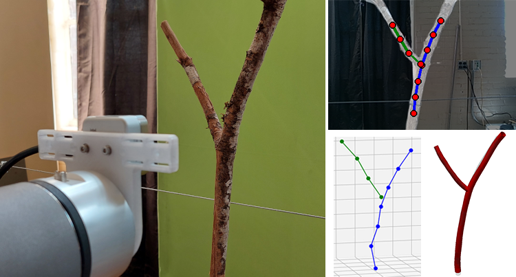
Figure 1: Our framework uses 2D RGB data and knowledge of the robot’s kinematics, camera intrinsics, and hand-eye calibration to follow along a primary branch and create highly accurate 3D branch reconstructions of the primary and secondary branches that can be used for making pruning decisions and executing cuts.

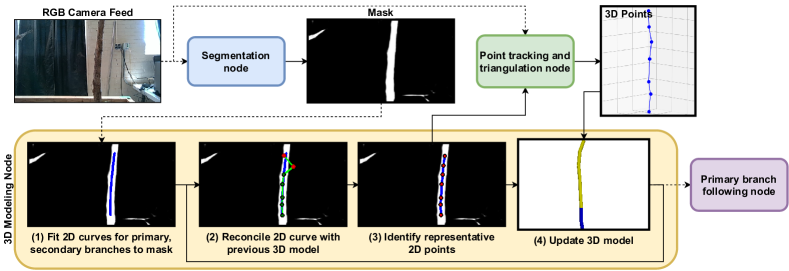
Figure 2: A system overview of our framework for branch scanning and reconstruction. It consists of 4 primary system nodes: A segmentation node producing binary masks; a point tracking node and triangulation node that reads in RGB images and returns 3D estimates for queried 2D pixels in an image; the core node that performs the branch reconstruction; and the controller node that moves the robot along the 3D primary branch. Dotted lines represent asynchronous system inputs.

In this paper, we introduce our framework (Fig. 1) designed to address the aforementioned limitations. Our system is capable of scanning up a primary branch, detecting secondary branches coming off of the primary branch, and creating 3D branch models that are accurate enough to be used for on the fly pruning decisions. The core components of the system are the controller that moves the camera on the robot’s end effector to follow a primary branch and the logic and active camera control for extracting the 3D geometry of the primary branch and its secondary branches. Our work is the first such work to focus on real-time modeling for close-up tree views where only a portion of the tree is visible. One benefit of this approach is that it uses an arbitrary off-the-shelf RGB camera mounted in an eye-in-hand configuration — no specialized stereo or RGB-D camera.

We evaluate our framework in both simulated and real environments and show that the 3D reconstruction is remarkably accurate, with an average primary branch position accuracy of 4mm, an average secondary branch orientation error of 15$\degree$, and a branch detection rate of 76% on a real robot. Furthermore, we can run at speeds of at least 10 cm/s without any noticeable loss of accuracy.

II Related Work

The problem of creating a topological model of a tree (or any 3D object) is known as skeletonization. We previously developed our own skeletonization algorithm [3] that uses semantic knowledge about a specific tree architecture, plus a convolutional neural network measuring connectedness between two points, to model the quality of the reconstruction. This objective function was used to search for an optimal reconstruction. Other methods also exist for apple trees [4, 5, 6], grapevines [7], jujube trees [8], and rose bushes [9]. All of these methods convert point clouds directly to skeletons, with the exception of  [7] that instead builds a 3D model by matching canes across 2D images (similar to our own work). Also of note is the method of [9] that adopts two key principles we also explore: segmentation masks to rectify 3D estimates and real-time algorithms. However, all of these methods focus on skeletonization of a full global scan of the corresponding plant, whereas our goal here is to focus on local branch reconstruction.

The approach we use is also inspired by structure from motion (SfM) techniques. These methods use a stream of 2D camera images with (potentially unknown) camera poses to create a 3D reconstruction of a scene by matching features between neighboring images and running an optimization method (bundle adjustment) to estimate the camera poses and construct the 3D scene. Such methods have been used for orchard-related applications such as fruit detection [10, 11], though none seem to exist for modeling tree branches. Although full SfM algorithms are often computationally expensive and output high density point clouds, they can be scaled down to track just a few points, as we do here.

Though not the main focus of the work, we also touch on active vision, i.e. using visual feedback to plan robot movement with the goal of maximizing information gain (detecting prunable branches). Our framework extends upon our previous Follow the Leader (FTL) controller [12] tasked with tracking a primary branch, though it did not perform 3D modeling of the primary and secondary branches. In the field of agri-food robotics, examples of similar work that locate objects of interest in the presence of occlusions using an eye-in-hand configuration can be found in [13] (greenhouse tomato localization) and [14, 15] (sweet pepper detection).

III System Design

Our work focuses on pruning in modern, high-density orchards. We assume that each tree architecture consists of primary branches (vertical or horizontal) and secondary side branches that grow perpendicularly off the primary branches. These side branches are candidates for pruning. Regardless of the specific fruit cultivar (e.g. apple, sweet cherry, currant, etc.), training system (V-trellis, spindle, UFO), or specific pruning rules, all share a need to search for secondary branches, model their locations, and execute cuts. The goals of our framework are to move the camera along the primary branch at a set distance of $z_{target}$, keep the branch centered in the camera’s view, and identify secondary branches coming off the primary branch. The output is a 3D branch reconstruction that captures the 3D geometry of the primary branch (skeleton and radius) along with the angle and position of the secondary branches.

A flow chart of our system is shown in Figure 2. The core component of our framework is the system that constructs the 3D skeleton of the tree using a stream of binary masks as input, which are produced by our segmentation framework. The 3D modeling node combines 2D information from the mask with 3D information from the point tracking and triangulation node to iteratively build a model of the scanned tree. The movement of the robot is handled by the primary branch following controller node that uses the existing 3D model to follow along the branch at a set distance.

Our segmentation system is described in detail in [16]. It produces masks by augmenting RGB images with optical flow and processing them through a generative adversarial network. For this paper, we focus on the other three novel components that allow for 3D perception of the scene as well as discovery of occluded branches.

IV 3D Branch Reconstruction

In this section, we discuss the subsystem that iteratively constructs the 3D model of the primary and secondary branches. Each branch model consists of a linear sequence of 3D points, as well as radius estimates at each point. The main steps are shown in the 3D Modeling Node box in Figure 2. At each iteration (which occurs after the robot has moved 10 mm from the last successful iteration), the modeling node takes in a segmentation mask and attempts to fit 2D Bézier curves for the primary and secondary branches and estimate their 2D radii (Figure 2, (1)); this operation is discussed below in Section IV-A. We then attempt to correct the existing 3D primary branch model by projecting it into the current image frame and checking if the projected points are consistent with the detected primary branch model (Figure 2, (2)), i.e. if at least 60% of the projected branch points are in the foreground mask and within 4 px of the 2D curve. There are several outcomes of the consistency-checking operation:

• (Consistent) All inconsistent 3D branch points (i.e. ones that are over 4 px away from the curve) are deleted from the model and reinitialized.

• (Inconsistent) We assume the mask data is bad and terminate processing of the existing mask.

• If we receive 3 inconsistent masks in a row, we assume the 3D model itself is wrong and delete all of the in-frame points from the 3D model. We then continue processing the existing mask.

Once we filter out inconsistent primary branch points, we then take the fit 2D primary Bézier curve and subsample it to a representative set of 2D pixels (Figure 2, (3)) by matching projected primary branch points to the closest pixel on the curve and adding new points to the model as they become visible, spacing out new points every 30 px. We then pass the 2D points through the point triangulation node (Section IV-B) to obtain 3D estimates of the points. We filter out bad 3D estimates by discarding those with a depth value above 1.0 m or a maximum reprojection error above 4 px. From the remaining points, we attempt to fit a 3D cubic Bézier curve using RANSAC with an inlier threshold of 3 cm. If the fit 3D curve has 60% inliers, we update the 3D primary branch model by averaging in inlier 3D points from the fit curve into their corresponding point in the 3D branch model (Figure 2, (4)). Furthermore, we estimate the 3D radius of each point as $zr_{px}/f$, where $z$ is the camera frame $z$-coordinate of the point, $r_{px}$ is the point’s corresponding 2D pixel radius estimate, and $f$ is the camera focal length.

We follow the same procedure with identified 2D secondary branch Bézier curves to yield 3D secondary branch models by matching each projected 3D secondary branch to a 2D Bézier curve, checking their consistency, feeding the representative 2D points through the point triangulation node, and fitting a 3D Bézier curve. Furthermore, to prevent adding background branches, we perform a check to verify that the 3D secondary branch actually intersects with the 3D primary branch by taking the ray at start of the secondary Bézier curve and checking if it comes within 3 cm of any edge in the primary model. If so, the branch is considered a match and is added to the list of secondary branches.

IV-A 2D curve fitting

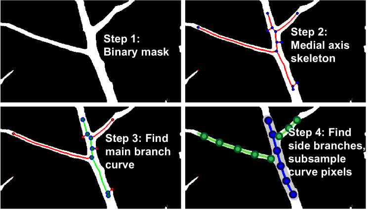
Figure 3: The process for extracting 2D primary and secondary branches from a skeleton. We start with the medial axis skeleton and find the subpath with the best fit to be the main branch. We then check skeletal paths extending off the primary branch to see if they are sufficiently long and a Bézier curve can be fit to them. We subsample the curves to identify pixels for which we will estimate 3D positions.

Figure 3 shows the process of locating the primary and secondary branch curves in a 2D mask. We start by using medial axis skeletonization [17] to obtain a pixel skeleton and radius estimates for each skeletal pixel. The pixel skeleton is then turned into a graph in which the nodes are all pixels at an endpoint (degree 1) or at a junction (degree 3 or above), with an edge between two nodes if they are connected by a linear segment of the skeleton (Step 2). These edges are oriented to point in the up ($-Y$) direction of the image, resulting in a multi-tree directed graph with no cycles.

To fit the primary Bézier curve, we run an exhaustive search of all possible pixel paths in the multi-tree (Step 3). For each pixel path, we perform a least squares regression to fit a cubic Bézier curve to the set of pixel points and select all inlier skeleton pixels that are within a given threshold (4 px) of the Bézier curve. The score of the pixel path is the size of the set of unique $y$-values of all inlier pixels. Once we have identified the highest scoring pixel path and associated Bézier curve $B(t)$, we subsample the curve to obtain representative 2D pixels (Step 4, blue curve) and match each subsampled pixel to the closest skeletal point to obtain its radius.

Once we identify the primary branch curve, we then identify all secondary branch curves. First, from the original (undirected) pixel skeleton graph, we identify all edges that are connected to the inside of the identified primary branch; these edges represent the starts of potential subpaths for secondary branches. For each edge, we run an exhaustive search like before to find the subpath with the best fitting Bézier curve. If the curve pixel length and the inlier rate is high enough, we add the detection to the set of “potential” secondary branches.

IV-B 3D triangulation via pixel tracking

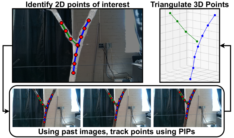
Figure 4: Using the Persistent Independent Particles point tracker, along with knowledge of the camera’s poses and intrinsics, we can obtain 3D estimates of an arbitrary subset of pixels in an image.

To obtain 3D point estimates from the identified 2D pixels, we use the Persistent Independent Particles (PIPs) method [18] to track a set of queried pixels over $M=8$ video frames, which are accumulated as the robot moves every 1.0 mm (Figure 4). We then combine each pixel’s trajectory with knowledge of the camera’s world frame pose and intrinsics at each frame to triangulate each pixel’s 3D coordinate.

Given a fixed camera calibration matrix $\mathbf{K}\in\mathbb{R}^{3\times 3}$ and a series of $M=8$ camera poses defined by rotation matrices $\mathbf{R}_{i}\in SO(3)$ and translations $T_{i}\in\mathbb{R}^{3}$, we obtain a series of projection matrices $\mathbf{P}_{i}=\mathbf{K}\begin{bmatrix}\mathbf{R}_{i}&T_{i}\end{bmatrix}\in\mathbb{R}^{3\times 4}$. Each projection matrix transforms homogeneous 3D points into 2D plus depth image coordinates. Denoting the rows of $\mathbf{P}_{i}$ as $\mathbf{p}_{i}^{1}$, $\mathbf{p}_{i}^{2}$, and $\mathbf{p}_{i}^{3}$, and given the list of $M$ pixel correspondences $(u,v)_{j,i}$ ($j$ keypoints for each of $i=M$ camera frames), we can define the matrix $\mathbf{D}_{j}\in\mathbb{R}^{2M\times 4}$ as follows:

$$\mathbf{D}_{j}=\begin{bmatrix}\mathbf{D}_{j,1}\\ \vdots\\ \mathbf{D}_{j,M}\end{bmatrix},\mbox{ where }\mathbf{D}_{j,i}=\begin{bmatrix}\left(u_{j,i}\mathbf{p}_{i}^{3}\right)-\mathbf{p}_{i}^{1}\\ \left(v_{j,i}\mathbf{p}_{i}^{3}\right)-\mathbf{p}_{i}^{2}\end{bmatrix}$$ (1)

The problem of finding a point $\mathbf{X}_{j}\in\mathbb{R}^{3}$ that minimizes the reconstruction error across all views is the same as finding a point $\mathbf{\underline{X}}_{j}\in\mathbb{R}^{4},\|\mathbf{\underline{X}}_{j}\|=1$ that minimizes the algebraic least-squares error $\|\mathbf{D}_{j}\mathbf{\underline{X}}_{j}\|^{2}$, which can be solved with singular value decomposition (SVD).

V 3D branch-following controller

In this section, we discuss the controller used to follow along the primary branch (Figure 5). This controller also performs the function of periodically rotating the camera around the primary branch, with the goal of gaining a view of branches that may be occluded by the original view.

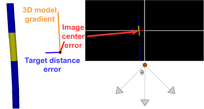
Figure 5: Components of the primary branch following controller. The controller follows the gradient of the model in front of the camera, with velocity offsets to keep a fixed distance from the branch and to keep the branch centered in the image (top-right). To gain a view of potentially occluded branches, it also periodically cycles through 3 camera orientations at an angle $\theta$ (bottom-right, shown from a top view).

To output the camera-frame velocity that tracks the primary branch, we use the 3D primary branch model described in the previous section. Supposing that the camera has an image width of $w$ and height $h$, we project the 3D primary branch model into the camera image frame and identify the pixel that falls closest to the vertical center at $\frac{h}{2}$. Let the identified pixel be $(u,v)$ with the corresponding camera frame 3D point $p=(x,y,z)$ having a gradient of $\nabla$. The formula for the velocity is a simple proportional controller with scaling factors $k_{u}$ for the horizontal pixel difference and $k_{z}$ for the target distance error (this velocity is subsequently scaled to a predetermined speed):

$$v_{tool}=\nabla+k_{u}\left(u-\frac{w}{2}\right)+k_{z}\left(z-z_{target}\right)$$ (2)

In addition, to gain a view of branches that are either directly in front of or behind the primary branch, the controller can also be configured to periodically rotate the camera by a given angle $\theta$ in the world $Z$-plane about $p$ after moving a set distance up in the world (Figure 5, bottom-right). It is useful to characterize this distance as a frequency with respect to the length of the camera’s vertical field of view at a distance of $z_{target}$; ideally the frequency should be greater than 1 to make sure the camera will not accidentally skip potentially occluded branches. Note that we disable mask generation while the camera is rotating since the optical flow-based segmentation scheme relies on translational camera movement for clean optical flow estimates.

VI Experiments

To validate the quality of the models produced by our framework, we performed experiments both in simulation and in a lab environment on real tree branches (Figure 6).

VI-A Simulated Experiments

The simulated experiment uses the Blender environment (Figure 6 left) to render a mock primary branch with secondary side branches. The primary branch is modeled as a randomized cubic Bézier curve extending from $z=0$ to $1$ meters in the world frame. Within the range of $z\in[0.325,0.75]$, we add side branches by uniformly sampling $z$-values and placing branches with random curvature at random orientations. The branch elevations are limited to $[-15\degree,45\degree]$, while the yaw can be any value.

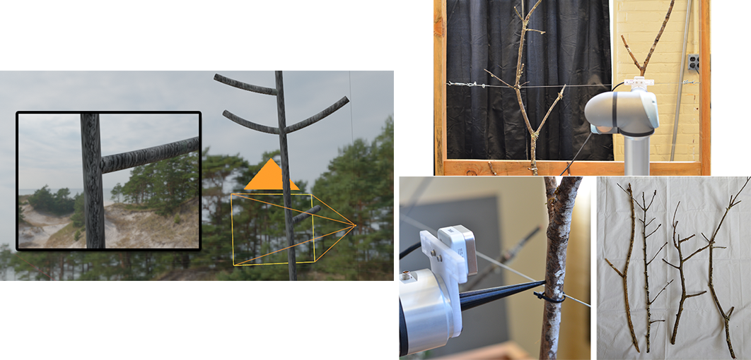
Figure 6: Setups used for evaluating our framework. Left: Our simulated Blender environment showing a mock spindle tree and a rendered camera image. Right: Our physical setup for the experiments (top), the detachable probe used to measure the ground truth (bottom-left), and the four branches we attempted to reconstruct (bottom-right).

The simulated robot is a UR5e manipulator (Universal Robots, Odense, Denmark) with a 320x240 camera coincident with the end effector frame. Each experiment started with sending the simulated robot to a home position at $z=0.275$ and running the framework until completion (the robot reaches $z=0.75)$ or failure (typically due to hitting a kinematic singularity).

To evaluate the ability of the controller to accurately detect branches and reconstruct their 3D geometry, we ran experiments with 5 different parameter sets for the branch-following controller. The baseline parameter set is no rotation in which the robot simply scans straight up the tree without changing its viewpoint. The other parameter sets add angular rotations of $\{22.5\degree,45\degree\}$ with rotation frequencies of $\{1.5,2.5\}$ per vertical FoV, which for our setup with a distance $z_{target}=0.20$ was 0.218 m.

VI-B Lab Experiments

The setup for the laboratory experiments is shown in Figure 6 (right). We utilize a UR5e with an Intel RealSense D405 camera mounted to the wrist flange. The experimental setup is designed to mimic a trellis-based environment similar to a real orchard. For each experiment, we secured a branch to the trellis and ran the system to extract a 3D model. To obtain “ground truth” data for the branch, we attached a probe to the robot and manually sampled the location of the surface of the primary and secondary branches. We also used digital calipers to record the radius at each sampled point.

The lab experiments follow the same procedure as the simulated ones. We ran our experiments for 4 different branches with 4 parameter sets: the baseline controller with no rotation at $\{0.02,0.05,0.10\}$ m/s, as well as the rotating controller with a lookat angle of $22.5\degree$ and 1.5 rotations per vertical FoV at $0.05$ m/s.

VII Results and Discussion

VII-A Simulated Experiments

	Simulated Experiments					Real Experiments
Lookat Angle °	0	22.5	45	22.5	45	22.5	0	0	0
Rotation Freq	0	1.5	1.5	2.5	2.5	1.5	0	0	0
Speed	N/A	N/A	N/A	N/A	N/A	0.05	0.02	0.05	0.10
PB Resid. (mm)	3.5 (4.0)	4.2 (4.9)	4.5 (8.9)	3.8 (3.7)	4.8 (7.5)	4.3 (4.6)	11.9 (15.9)	6.5 (13.1)	4.7 (7.5)
PB Rad. Error %	6 (10)	5 (9)	6 (9)	5 (7)	6 (9)	18 (15)	16 (31)	16 (18)	19 (18)
SB $\angle$ Error °	13 (8)	16 (11)	15 (9)	15 (10)	17 (10)	13 (8)	17 (13)	11 (5)	15 (6)
SB Detection %	91	95	91	95	91	76	76	73	76
SB Len Error %	5 (91)	11 (84)	-4 (32)	4 (75)	4 (51)	N/A	N/A	N/A	N/A
SB Rad. Error %	-13 (16)	-13 (15)	-12 (16)	-12 (15)	-11 (13)	N/A	N/A	N/A	N/A

TABLE I: Results of the simulated and real experiments for each parameter set (PB = primary branch, SB = secondary branch, Resid = residual, Rad. = radius). Standard deviation values are given in parentheses.

Table I shows a summary of the experiments (simulated and real), and Figure 7 shows some sample reconstructions. First, we focus on the results of the baseline controller with no rotation before analyzing the results of adding rotation. As a whole, the reconstruction accuracy of the framework was remarkably accurate, with the average primary branch residual (i.e. the distance from the constructed model at a given $z$-value to the corresponding ground truth model) of just 3.5mm and an average radius estimate error of 6.4%. These values were generally positively skewed, characterized by infrequent but large outliers.

Meanwhile, considering the secondary branches, we were able to positively detect almost 91% of all secondary branches, even without rotating the camera to get new views. Typically, the branches that were missed were either pointing straight towards or away from the camera. For the branches that were detected, the average orientation error from the ground truth was 13.1 degrees, a value that is more than sufficient for pruning. Radius estimation was also reasonably accurate with an average of -13%. One area that requires significant improvement is length estimation; though the average error was 5.2%, the standard deviation was 90.7%. Large errors tended to have two causes: Either a background point was selected for 3D estimation and not filtered out, or poor 3D estimates in the secondary branch caused the cubic Bézier curve to have an unusual shape with sharp bends. Though the length estimation was by far the weakest part of the framework, it is also not as essential for the pruning task as detection and estimation of orientation.

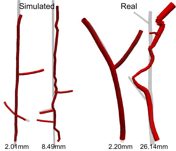
Figure 7: Examples of 3D reconstructions of the branches from the framework with the corresponding primary branch residual values. The ground truth is faded while the reconstructed model is shown in red.

The effects of adding rotation to the controller were mixed. First, there were not any notable differences between the two rotation frequencies (1.5 and 2.5), indicating that 1.5 is preferred since the robot will spend less time rotating the camera. Regarding the different rotation angles, there was a slight increase in branch detection rate using the 22.5 degree value, which is expected since the robot should be able to spot branches that initially point directly toward or away from the camera. Surprisingly, this advantage disappeared when increasing the rotation to 45 degrees. Indeed, doubling the rotation generally reduced the accuracy metrics and also led to a few instances where the manipulator became stuck in a singularity. The one advantage the 45 degree controller had was in reducing the magnitude of the length errors of the secondary branches, since the robot was able to gain a more clear view of poorly detected secondary branches and remove sections of the model that were not in the mask. As a whole, the metrics for the controllers with rotation were not notably statistically different than those of the baseline. Despite this, the results do support our initial motivation of incorporating multiple viewpoints to discover hidden branches.

One other notable weakness in secondary branch detection was redetecting the same branch multiple times. We did incorporate some heuristics such as branch origin location and orientation to detect if a 3D secondary curve was the same as a previous one, but there was still an “overdetection” rate of 32%. Despite this, it was quite rare for the system to have completely spurious secondary branch detections, with a rate of just 4%.

VII-B Real Experiments

Due to the difficulty of manually probing the entire tree, we focus on a subset of metrics for the real experiments: The primary branch residual and radius errors as well as the secondary branch detection and orientation estimates. In comparison to the simulated data, there were higher primary residuals and radius errors on real branches. The main source of the higher residuals is from instances in which a model point was incorrectly projected into the background and was never corrected (e.g. Figure 7). Unlike with the simulated experiments, including rotation in the controller significantly reduced the presence of large residuals caused by poor 3D estimates since the system could detect such errors as inconsistent with the mask and correct them.

For the secondary branches, compared to the simulated experiments, the detection rate was lower at about 76% and the orientation errors had roughly the same magnitude. The primary cause of the lower success rate was the real branches being thinner and irregularly shaped. Another major contributor was that the background wall was closer to the robot than the background in the simulated environment, which caused the masks to be noisier. This led to issues with spurious branch detections and situations where secondary branches were poorly modeled due to failing to properly filter out points projected into the background.

There was no significant difference between the performance of the controllers based on speed. Somewhat surprisingly, the primary branch residuals decreased as speed increased. This likely has to do with the point triangulation node, which is set to acquire 8 images over a minimum distance of 7.5 mm. However, at a speed of 10 cm/s with a frame rate of 30 images per second, the distance covered would be 26.7 mm. It is likely that the images being further apart contributes to more reliable 3D point estimates (or makes bad 3D point estimates easier to detect).

VII-C Runtime

We used a computer with an i7-11800H 8-core processor and an NVIDIA GeForce RTX 3060 Laptop GPU, running ROS2 Humble on Ubuntu 22.04. With this setup and 320x240 image inputs, the average runtimes to process one input for each node were:

• Segmentation node: 0.037 s (26.9 Hz)

• 3D curve modeling node: 0.146 s (6.8 Hz). This runtime includes the synchronous call to the point tracking and triangulation node, which took 0.068 s (14.6 Hz)

• Primary branch following node: 0.00011 s (9300 Hz)

Even with unoptimized Python code, it is clear that the pipeline is suitable for real-time use, with the main bottleneck (the 3D curve modeling node) still running nearly seven times per second. The limiting speed of the system (not accounting for practical effects such as motion blur or vibration) would correspond to a speed such that the end effector would move over 1 vertical FoV during the curve processing time, which for our setup would be about 1.5 m/s (much faster than we would desire to run the system).

VIII Conclusion

In this paper, we introduced a framework for scanning along a primary branch while constructing a model of the branch, motivated by the need to quickly and efficiently locate prunable secondary branches and the corresponding 3D estimates of their cut points. By combining traditional 2D skeletonization methods with deep neural networks for segmentation and 3D point estimation, we developed a system that can create accurate branch models while running at practical speeds. This work represents a useful framework for pruning locally, on-the-fly without the need for a global reconstuction of the plant.

There are many notable improvements that could be made to the system. The first is the branch modeling, since the current method of projecting the previous tree model into the current mask and deleting parts of the model that repeatedly fail to project inside the mask is overly simplistic. A more rigorous approach would be to use a probabilistic particle model, such as those used in 3D SLAM algorithms, to keep track of each branch point estimate. Another aspect that could be improved is the rotation to discover new branches, which currently occurs at a fixed frequency. To reduce the amount of time spent rotating the camera, it would be useful for the system to perform rotation only when it identifies the possible presence of a new branch but needs a better view of it. Finally, there is currently no consideration for avoiding detected branches or kinematic singularities. For a practical implementation, it will be essential for the system to be able to plan kinematically feasible paths to avoid hitting front-facing branches.

References

- [1] A. Zahid, M. S. Mahmud, L. He, P. Heinemann, D. Choi, and J. Schupp, “Technological advancements towards developing a robotic pruner for apple trees: A review,” Computers and Electronics in Agriculture, vol. 189, p. 106383, Oct. 2021.
- [2] A. You, N. Parayil, J. G. Krishna, U. Bhattarai, R. Sapkota, D. Ahmed, M. Whiting, M. Karkee, C. M. Grimm, and J. R. Davidson, “Semiautonomous precision pruning of upright fruiting offshoot orchard systems: An integrated approach,” IEEE Robotics & Automation Magazine, pp. 2–11, 2023.
- [3] A. You, C. Grimm, A. Silwal, and J. R. Davidson, “Semantics-guided skeletonization of upright fruiting offshoot trees for robotic pruning,” Computers and Electronics in Agriculture, vol. 192, p. 106622, 2022.
- [4] M. Karkee and B. Adhikari, “A method for three-dimensional reconstruction of apple trees for automated pruning,” Transactions of the ASABE, vol. 58, no. 3, pp. 565–574, 2015.
- [5] S. A. Akbar, N. M. Elfiky, and A. Kak, “A novel framework for modeling dormant apple trees using single depth image for robotic pruning application,” in 2016 IEEE International Conference on Robotics and Automation (ICRA). IEEE, 2016, pp. 5136–5142.
- [6] A. Bucksch and R. Lindenbergh, “Campino—a skeletonization method for point cloud processing,” ISPRS Journal of Photogrammetry and Remote Sensing, vol. 63, no. 1, pp. 115–127, 2008.
- [7] T. Botterill, S. Paulin, R. Green, S. Williams, J. Lin, V. Saxton, S. Mills, X. Chen, and S. Corbett-Davies, “A robot system for pruning grape vines,” Journal of Field Robotics, vol. 34, no. 6, pp. 1100–1122, 2017.
- [8] Y. Fu, Y. Xia, H. Zhang, M. Fu, Y. Wang, W. Fu, and C. Shen, “Skeleton extraction and pruning point identification of jujube tree for dormant pruning using space colonization algorithm,” Frontiers in Plant Science, vol. 13, p. 1103794, 2023.
- [9] H. Cuevas-Velasquez, A.-J. Gallego, and R. B. Fisher, “Segmentation and 3d reconstruction of rose plants from stereoscopic images,” Computers and electronics in agriculture, vol. 171, p. 105296, 2020.
- [10] J. Gené-Mola, R. Sanz-Cortiella, J. R. Rosell-Polo, J.-R. Morros, J. Ruiz-Hidalgo, V. Vilaplana, and E. Gregorio, “Fruit detection and 3d location using instance segmentation neural networks and structure-from-motion photogrammetry,” Computers and Electronics in Agriculture, vol. 169, p. 105165, 2020.
- [11] X. Liu, S. W. Chen, S. Aditya, N. Sivakumar, S. Dcunha, C. Qu, C. J. Taylor, J. Das, and V. Kumar, “Robust fruit counting: Combining deep learning, tracking, and structure from motion,” in 2018 IEEE/RSJ international conference on intelligent robots and systems (IROS). IEEE, 2018, pp. 1045–1052.
- [12] N. Parayil, A. You, C. Grimm, and J. Davidson, “Follow the leader: a path generator and controller for precision tree scanning with a robotic manipulator,” in Precision agriculture’23. Wageningen Academic, 2023, pp. 167–174.
- [13] D. Rapado-Rincón, E. J. van Henten, and G. Kootstra, “Development and evaluation of automated localisation and reconstruction of all fruits on tomato plants in a greenhouse based on multi-view perception and 3d multi-object tracking,” Biosystems Engineering, vol. 231, pp. 78–91, 2023.
- [14] R. Barth, J. Hemming, and E. J. van Henten, “Design of an eye-in-hand sensing and servo control framework for harvesting robotics in dense vegetation,” Biosystems Engineering, vol. 146, pp. 71–84, 2016.
- [15] C. Lehnert, D. Tsai, A. Eriksson, and C. McCool, “3d move to see: Multi-perspective visual servoing towards the next best view within unstructured and occluded environments,” in 2019 IEEE/RSJ International Conference on Intelligent Robots and Systems (IROS). IEEE, 2019, pp. 3890–3897.
- [16] A. You, C. Grimm, and J. R. Davidson, “Optical flow-based branch segmentation for complex orchard environments,” in 2022 IEEE/RSJ International Conference on Intelligent Robots and Systems (IROS). IEEE, 2022, pp. 9180–9186.
- [17] H. Blum, “A transformation for extracting new descriptions of shape,” Models for the perception of speech and visual form, pp. 362–380, 1967.
- [18] A. W. Harley, Z. Fang, and K. Fragkiadaki, “Particle video revisited: Tracking through occlusions using point trajectories,” in ECCV, 2022.