Constraints between entropy production and its fluctuations in nonthermal engines

Abstract

We analyze a mesoscopic conductor autonomously performing a thermodynamically useful task, such as cooling or producing electrical power, in a part of the system—the working substance—by exploiting another terminal or set of terminals—the resource—that contains a stationary nonthermal (nonequilibrium) distribution. Thanks to the nonthermal properties of the resource, on average no exchange of particles or energy with the working substance is required to fulfill the task. This resembles the action of a demon, as long as only average quantities are considered. Here, we go beyond a description based on average currents and investigate the role of fluctuations in such a system. We show that a minimum level of entropy fluctuations in the system is necessary, whenever one is exploiting a certain entropy production in the resource terminal to perform a useful task in the working substance. For concrete implementations of the demonic nonthermal engine in three- and four-terminal electronic conductors in the quantum Hall regime, we compare the resource fluctuations to the entropy production in the resource and to the useful engine output (produced power or cooling power).

I Introduction

The rapidly evolving research field of quantum thermodynamics is constantly pushing the boundaries of our understanding of thermodynamic processes at the nanoscale Binder et al. (2018); Strasberg (2022). In contrast to macroscopic systems, which are typically well described by average quantities, small-scale devices are very much influenced by fluctuations Esposito et al. (2009); Seifert (2008) and often possess quantum features, requiring the standard thermodynamic laws to be modified and complemented by additional concepts, for example borrowed from information theory. Besides the fundamental challenge of establishing a thermodynamically consistent description of nanoscale systems, understanding their behavior leads to potential practical applications. A prominent example is that of heat management and energy conversion in nanoelectronics Benenti et al. (2017), with an ever increasing relevance due to the miniaturization opportunities offered by technological developments.

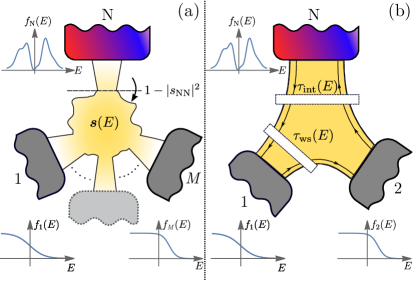
Figure 1: (a) Generic multi-terminal electronic conductor fed by a nonthermal resource (N) with distribution $0\leq f_{\text{N}}(E)\leq 1$. The properties of the coherent conductor are encoded in the scattering matrix $\bm{s}(E)$. In particular, the resource region (above the horizontal dashed line) is connected to the working substance (below the dashed line) by the transmission probability $1-|s_{\text{NN}}(E)|^{2}$. (b) Minimal setup exploiting a nonthermal resource in a a 3-terminal quantum Hall device. The resource is connected to the working substance by the interface transmission probability $\tau_{\text{int}}(E)$ and power production is enabled by the energy-dependent transmission $\tau_{\mathrm{ws}}(E)$.

Among the exciting features of small-scale systems is the possibility to access non-conventional resources that can be used to power nanoscale engines, in addition to heat and work. It is for instance interesting to understand the role of quantum coherences Scully et al. (2003); Francica et al. (2017); Niedenzu et al. (2018); Ghosh et al. (2019), as well as that of information Bennett (1982); Bérut et al. (2012); Parrondo et al. (2015) or of active matter Krishnamurthy et al. (2016); Holubec et al. (2020); Pietzonka et al. (2019). Here, we focus on another option, namely to exploit a terminal that supplies a steady-state fermionic resource that is nonthermal (nonequilibrium) Abah and Lutz (2014); Tesser et al. (2023a). It hence does not possess a well-defined temperature or potential, as depicted in Fig. 1(a). While this contradicts the standard notion of a bath or a reservoir, it is a quite common situation in nanoscale systems that might interact with different environments and that can have themalization lengths exceeding the system size Benenti et al. (2017). Also time-dependent nonequilibrium states can be available Strasberg et al. (2017); Konopik et al. (2020); Ryu et al. (2022). Moreover, it is likely that such nonthermal resources are present in nanoscale systems, as they may originate as a “waste” byproduct of other processes of interest. Understanding how such nonthermal distributions can be harvested is hence expected to be relevant from a practical point of view.

In previous works Whitney et al. (2016); Sánchez et al. (2019), some of us have introduced the concept of a nonequilibrium demon (N-demon). Such a system is able to perform a useful task in a steady-state operation by solely relying on a nonthermal (nonequilibrium) resource, in the absence of average heat or work consumption, namely neither average energy nor average particle currents flow between the resource region and the working substance, see Fig. 1. This resembles a Maxwell demon Esposito and Schaller (2012); Strasberg et al. (2013); Koski et al. (2014a, 2015); Chida et al. (2017); Masuyama et al. (2018); Sánchez et al. (2019); Freitas and Esposito (2021a); Bozkurt et al. (2022); Saha et al. (2023)—hence the choice of the name N-demon Whitney (2023)—but the working principle is very different as it does not rely on any type of feedback and is “demonic” only when focusing on average quantities. This has triggered a number of related works, where various properties of systems relying on nonequilibrium resources have been analyzed Deghi and Bustos-Marún (2020); Ciliberto (2020); Hajiloo et al. (2020); Lu et al. (2021). In particular, it has been shown that a performance characterization of an N-demon Deghi and Bustos-Marún (2020); Hajiloo et al. (2020) can be achieved by introducing well-behaved free-energy efficiencies Manzano et al. (2020); Hajiloo et al. (2020); Tesser et al. (2023a) taking into account that a nonthermal resource is exploited.

The absence of feedback mechanisms in an N-demon suggests that fluctuations play a fundamental role for the operation of engines exploiting nonthermal resources Freitas and Esposito (2021b). However, while noise in the absence of charge or heat currents has recently attracted a lot of interest in systems with standard thermal reservoirs Lumbroso et al. (2018); Larocque et al. (2020); Eriksson et al. (2021); Tesser et al. (2023b), previous studies on nonthermal engines have addressed average quantities only. The characterization of fluctuations of nonthermal resources for the operation of nanoscale engines in general, and for N-demons more specifically, is the gap we aim to fill with the present paper. More concretely, we quantify to what extent the fluctuations associated with temporary exchanges of particles and energy between the resource and the working substance relate to the performance of this autonomous (steady-state) device. In this paper, we identify that the entropy reduction in the working substance, and hence the entropy production in the resource region, requires a minimum level of fluctuations. We find that it is a combination of entropy and particle fluctuations that sets the constraint. This key result reads

$$S_{\text{NN,cl}}^{\Sigma}{+}\frac{k_{\text{B}}^{2}}{4}S_{\text{NN,cl}}\geq 2k_{\text{B}}I^{\Sigma}_{\rm N}\geq-2k_{\text{B}}I^{\Sigma}_{\rm ws},$$ (1)

where $I^{\Sigma}_{\text{N}}$ is the entropy production in the nonthermal resource, $-I^{\Sigma}_{\text{ws}}$ is the entropy reduction in the working substance (quantifying the useful output), where both the resource and working substance contain one or more fermionic steady-state contacts. The terms on the left-hand side characterize the entropy and particle fluctuations in the nonthermal resource (see Sec. III for definitions and details of the introduced quantities). We refer to this sum as the classical part of the resource fluctuations in the following. For systems with thermal contacts only, this results in constraints involving heat and particle fluctuations. In this paper, we derive Eq. (1) and illustrate its implications with specific examples. More specifically, we apply our findings, that are valid for arbitrary noninteracting multi-terminal conductors with possibly nonthermal resources, to 3- or 4-terminal N-demon systems realized in the quantum Hall regime. In conductors in the quantum Hall regime, the time-reversal symmetry breaking in chiral edge states Büttiker (1988) allows for particularly simple implementations of quantum conductors for energy conversion Sánchez et al. (2015) and for the inspection of current-current correlations Texier and Büttiker (2000). In experimental implementations of such systems, detection of nonthermal distributions Altimiras et al. (2010), of heat flow Jezouin et al. (2013), and of noise Sivre et al. (2019) have been demonstrated, making them relevant for our purpose. We identify situations in which the noise is particularly small, approaching the discovered bound, Eq. (1). For specific, experimentally relevant implementations of N-demons in quantum Hall conductors, namely where either the nonthermal distribution allows one to get close to the identified bound or where the nonthermal distribution is engineered by a coherent mixing of thermal resources, we analyze the resource fluctuations and how they are related to the maximum power or cooling power that can be achieved in the device.

This paper is structured as follows: We introduce the model and the employed scattering approach for all analyzed quantities, including the entropy currents and their fluctuations, in Sec. II. We then demonstrate that they are related to each other in a general way by constraints on entropy fluctuations compared to entropy flow in Sec. III. In Sec. IV, we provide the shape that these constraints take for a three-terminal quantum Hall setup and analyze their implications. Finally, results for resource fluctuations in a specific 4-terminal setup, where the nonthermal distribution is engineered, are presented in Sec. V. The Appendices contain analytical expressions in limiting regimes as well as derivations and results for the four-terminal setup, where the nonthermal distribution is injected from a resource consisting of a set of thermal contacts, complementing the ones in the main paper.

II Model and thermodynamic transport quantities

II.1 Multi-terminal conductor

We consider a generic multi-terminal coherent electronic conductor, as sketched in Fig. 1(a). The upper terminal, denoted by N, is in a nonthermal state and provides the resource exploited by the working substance—a coherent conductor with $M$ standard thermal reservoirs, denoted by $1,2,\dots M$. The task of the device is to exploit the resource provided by the nonthermal terminal to produce in a steady-state operation a useful output in the working substance, such as extracting electrical power between any two contacts or cooling one of the contacts by transporting heat into a hotter contact. In general, the device does something useful whenever the entropy of the working substance is reduced, at the expense of an increase in the entropy of the resource region. In this Section and in Sec. III, we will keep the treatment as general as possible, while a minimal model based on a three-terminal device, sketched in Fig. 1(b), will be presented in Sec. IV.

The theoretical framework we rely on is a scattering matrix approach Blanter and Büttiker (2000); Moskalets (2011), valid for coherent conductors in which many-body interactions are negligibly small. We emphasize that, interactions being absent, we can exclude that any autonomous feedback mechanisms Strasberg et al. (2013); Koski et al. (2014a); Whitney et al. (2016); Sánchez et al. (2019) play a role in our device, so that any “demonic” effects, appearing in the absence of average charge energy flow between resource and working substance, can safely be attributed to the presence of the nonthermal resource.

The energy-dependent scattering matrix $\bm{s}(E)$ describes the conductor’s properties, where the matrix element $s_{\alpha\beta}(E)$ gives the probability amplitude that an electron emitted at energy $E$ by terminal $\beta$ is transmitted into terminal $\alpha$. The energy dependence of the scattering matrix is typically tunable by gates in mesoscopic electronic conductors. The terminals are characterized by distribution functions denoted by $f_{\alpha}(E)$, with $\alpha=1,2,\dots M,\text{N}$. For a standard equilibrium contact, we have a Fermi function

$$f_{\alpha}(E)=\frac{1}{1+\exp[\beta_{\alpha}(E-\mu_{\alpha})]},\quad\alpha\neq\text{N},$$ (2)

with inverse temperature $\beta_{\alpha}=1/k_{\text{B}}T_{\alpha}$ and electrochemical potential $\mu_{\alpha}$. In contrast, $f_{\text{N}}(E)$ is a generic function describing the nonthermal terminal N. It is only constrained by $0\leq f_{\text{N}}(E)\leq 1$, as it represents the occupation probability of an electronic (fermionic) contact.

II.2 Charge, heat and entropy currents and fluctuations

The average, steady-state currents flowing into terminal $\alpha$ can be found as the expectation values of the fluctuating current operators as provided in Appendix A and are given by Blanter and Büttiker (2000); Moskalets (2011)

$$I^{X}_{\alpha}=\braket{\hat{I}_{\alpha}^{X}}=\frac{1}{h}\int dE\,x_{\alpha}\sum_{\beta}|s_{\alpha\beta}(E)|^{2}[f_{\beta}(E)-f_{\alpha}(E)]\,.$$ (3)

Here, we use the abbreviation $X$ in order to indicate different types of currents, with $(X,x_{\alpha})\in\left\{(\emptyset,1),(\mathrm{E},E),(\Sigma,k_{\text{B}}\sigma_{\alpha})\right\}$. This includes the particle current $I_{\alpha}$ and the energy current $I^{\mathrm{E}}_{\alpha}$. The average heat current $J_{\alpha}$, for $\alpha\neq\text{N}$, is consequently given by

$$J_{\alpha}=I^{\mathrm{E}}_{\alpha}-\mu_{\alpha}I_{\alpha}\,.$$ (4)

In addition to charge, energy, and heat currents, we are interested in the entropy production in a given terminal. In this steady-state coherent conductor, this is given by the entropy current into contact $\alpha$, namely $I^{\Sigma}_{\alpha}$, with

$$\sigma_{\alpha}(E)\equiv-\log\left[\frac{f_{\alpha}(E)}{1-f_{\alpha}(E)}\right],$$ (5)

see Ref. Deghi and Bustos-Marún (2020) or Appendix A for different derivations of the entropy current. This entropy current $I^{\Sigma}_{\alpha}$ properly reduces to Clausius’ relation

$$I^{\Sigma}_{\alpha}\rightarrow I_{\alpha}^{\Sigma,\mathrm{thermal}}=\frac{J_{\alpha}}{T_{\alpha}}\,,$$ (6)

valid for thermal contacts, when $f_{\alpha}$ is a Fermi function, i.e., $\alpha\neq\mathrm{N}$. Moreover, it is a thermodynamically consistent quantity, as it satisfies the second law, $\sum_{\alpha}I^{\Sigma}_{\alpha}\geq 0$, even when all contacts have nonthermal occupation probabilities Whitney (2023). This formulation for the entropy production requires the nonthermal contact to be a large, macroscopic electronic system without any classical or quantum correlations, referred to as “nonequilibrium incoherent reservoir” by the authors of Ref. Deghi and Bustos-Marún (2020).

We mention that a different formulation of entropy production has been introduced in Ref. Bruch et al. (2018), in situations possibly involving time-dependent drivings. There, however, the authors are concerned with the entropy production associated with the scattering states in the coherent leads, as opposed to the one referring to the macroscopic contacts that we are considering here. The difference is that by looking at the outgoing states in the leads only, any equilibration process happening when the electrons enter the macroscopic contact is not taken into account.

We refer to the multi-terminal system introduced above as an N-demon and to the resource region as “demonic”, whenever the system obeys the strict demon conditions on the currents

$$I_{\text{N}}=I^{\mathrm{E}}_{\text{N}}=0\,.$$ (7)

This enforces that no exchange of particles or energy between the working substance and the resource region happens on average. In this case, any useful output generated in the working substance is obtained without the consumption of an average energy resource and the resource is characterized by entropy flows or by free energies Hajiloo et al. (2020). Even though Eq. (7) rules out any net transfer of particles and energy, these quantities can still fluctuate. We will show in this paper that such fluctuations must be present in order for the nonthermal resource to produce a useful output under the strict demon conditions.

The zero-frequency noise related to any of the currents $I_{\alpha}^{X}$ considered here is defined by the correlator

$$S_{\alpha\beta}^{X}=\int_{-\infty}^{+\infty}dt\Braket{\{\delta\hat{I}_{\alpha}^{X}(t),\delta\hat{I}_{\beta}^{X}(0)\}},$$ (8)

where $\delta\hat{I}_{\alpha}^{X}=\hat{I}_{\alpha}^{X}-I_{\alpha}^{X}$ are the fluctuations of the current with respect to its average, steady-state value, see Appendix A for the definitions of the relevant fluctuating current operators. For the general case sketched in Fig. 1(a), these quantities evaluate to $S_{\alpha\beta}^{X}=S_{\alpha\beta,\text{cl}}^{X}+S_{\alpha\beta,\text{qu}}^{X}$, with Moskalets (2011); Nazarov and Blanter (2009); Blanter and Büttiker (2000)

$$\begin{split}S_{\alpha\beta,\text{cl}}^{X}&\equiv\frac{2}{h}\int dE\,x_{\alpha}x_{\beta}\Big{\{}-F_{\alpha\alpha}|s_{\beta\alpha}|^{2}-F_{\beta\beta}|s_{\alpha\beta}|^{2}\\ &\quad+\delta_{\alpha\beta}\sum_{\gamma}|s_{\alpha\gamma}|^{2}[F_{\alpha\gamma}+F_{\gamma\alpha}]\Big{\}}\,,\end{split}$$ (9a)

$$\begin{split}S_{\alpha\beta,\text{qu}}^{X}\equiv-\frac{2}{h}\int dE\,x_{\alpha}x_{\beta}&\Re\Big{\{}\Big{[}\sum_{\gamma}(f_{\alpha}-f_{\gamma})s^{*}_{\alpha\gamma}s_{\beta\gamma}\Big{]}\\ &\times\Big{[}\sum_{\gamma}(f_{\beta}-f_{\gamma})s_{\alpha\gamma}s_{\beta\gamma}^{*}\Big{]}\Big{\}}.\end{split}$$ (9b)

Here, the total noise has been split into classical-like and quantum contributions. The classical-like part contains all the linear terms in the scattering probabilities $|s_{\alpha\beta}|^{2}$ and describes one-particle transfers across the conductor. It can be seen as a generalization of a fully classical expression with the addition of Pauli-blocking factors $F_{\alpha\beta}\equiv f_{\alpha}(1-f_{\beta})$ implementing the exclusion principle Brandner et al. (2018); Liu and Segal (2019); Kirchberg and Nitzan (2022) (further quantum effects can still influence the form of $|s_{\alpha\beta}|^{2}$). The quantum part, in contrast, involves correlated two-particle processes. Note that the division of noise into separate meaningful contributions is obviously not unique Büttiker (1992); Blanter and Büttiker (2000); for the situation studied here, the separation into quantum and classical contributions turns out to be favourable. In Eq. (9), we have omitted for convenience the energy dependence of the scattering matrix elements $s_{\alpha\beta}(E)$ and of the distribution functions $f_{\alpha}(E)$.

In what follows, a relevant role will be played by the entropy fluctuations $S_{\alpha\beta}^{\Sigma}$ for generic, thermal or nonthermal occupation probabilities $f_{\alpha}$ and $f_{\beta}$. For entropy fluctuations between terminals $\alpha$ and $\beta$ with thermal distributions, these fluctuations are nothing but the correlation functions $\braket{\delta\hat{J}_{\alpha}\delta\hat{J}_{\beta}}/(T_{\alpha}T_{\beta})$ of the heat currents, divided by the corresponding temperatures of terminals $\alpha$ and $\beta$. We stress that a straightforward connection between the entropy and heat can be obtained in the thermal case only. When contacts with nonthermal occupation probabilities are involved, inferring the entropy production necessarily relies on the knowledge of the nonthermal distributions themselves. While this can be a challenging task, it has been shown that such nonequilibrium distributions can be experimentally accessed via spectroscopy techniques Altimiras et al. (2010).

III General bound on local entropy fluctuations

We are now in a position to answer the question raised in the introduction: What is the minimum amount of fluctuations of the resource currents (possibly with zero average) required for the production of a useful output in the working substance?

We here identify the entropy production and its fluctuations as well as the particle current fluctuations, as the relevant quantities which constrain each other. Specifically, for the autocorrelations of the entropy currents in any terminal $\alpha$, $S_{\alpha\alpha}^{\Sigma}=S_{\alpha\alpha,\text{cl}}^{\Sigma}+S_{\alpha\alpha,\text{qu}}^{\Sigma}$, one has for the classical and quantum parts

$$\begin{split}S_{\alpha\alpha,\text{cl}}^{\Sigma}=&\frac{2k_{\text{B}}^{2}}{h}\int dE\,\left[\sigma_{\alpha}\right]^{2}\sum_{\gamma\neq\alpha}|s_{\alpha\gamma}|^{2}(F_{\alpha\gamma}+F_{\gamma\alpha}),\end{split}$$ (10a)

$$S_{\alpha\alpha,\text{qu}}^{\Sigma}= -\frac{2k_{\text{B}}^{2}}{h}\int dE\,\Big{[}\sigma_{\alpha}\sum_{\gamma\neq\alpha}|s_{\alpha\gamma}|^{2}(f_{\alpha}{-}f_{\gamma})\Big{]}^{2}.$$ (10b)

To establish bounds on the entropy production imposed by these fluctuations, we use the following inequalities that are valid independently of whether the distributions $f_{\alpha},f_{\gamma}$ are thermal or not:

$$\left|\sigma_{\alpha}\right| \leq\left[\sigma_{\alpha}\right]^{2}+\frac{1}{4}\,,$$ (11a)

$$|f_{\alpha}-f_{\gamma}| \leq F_{\alpha\gamma}+F_{\gamma\alpha}\ .$$ (11b)

To get some intuition about these inequalities, we illustrate in Fig. 2 under which conditions they turn into equalities, for the simple case where the functions $f_{\alpha}$ and $f_{\beta}$ are Fermi functions. Using (11), we find that the classical component of the noise satisfies

$$S_{\alpha\alpha,\text{cl}}^{\Sigma}{+}\frac{k_{\text{B}}^{2}}{4}S_{\alpha\alpha,\text{cl}} \geq\frac{2k_{\text{B}}^{2}}{h}\int dE\left|{\sigma_{\alpha}}\sum_{\gamma}|s_{\alpha\gamma}|^{2}(f_{\alpha}-f_{\gamma})\right|$$

$$\geq 2k_{\text{B}}|I^{\Sigma}_{\alpha}|.$$ (12)

This is the first key result of this paper; it relates the entropy production to a combination of the classical contributions to entropy and particle fluctuations, which reduces to a combination of the classical contributions to heat and charge fluctuations in the case of thermal contacts. We are in particular interested in the fluctuations of the nonthermal resource, where the relation (III) provides us with a relevant definition of the classical part of resource fluctuations,

$$S_{\text{res,cl}}\equiv S_{\text{NN,cl}}^{\Sigma}+\frac{k_{\text{B}}^{2}}{4}S_{\text{NN,cl}}\,,$$ (13)

that will be used later to characterize the N-demon. We will show in Sec. IV.2 under which conditions the bound set by the generally valid inequality (III) can be approached in a concrete device realization, even when in addition the strict demon conditions (7) are imposed.

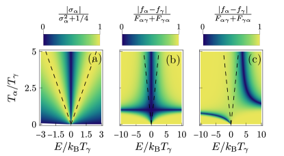
Figure 2: Illustration of the inequalities (11) for simple Fermi functions. We set $\mu_{\alpha}\equiv 0$ as the reference energy and plot the ratios of the left and right hand side of Eqs. (11) as function of energy and of the ratio of temperatures $T_{\alpha}/T_{\gamma}$. (a) Plot of $|\sigma_{\alpha}|/[\sigma_{\alpha}^{2}+1/4]$ demonstrating that Eq. (11a) is saturated around $E-\mu_{\alpha}=\pm k_{\text{B}}T_{\alpha}/2$, as highlighted by the dashed lines. (b-c) Plots of $|f_{\alpha}-f_{\gamma}|/(F_{\alpha\gamma}+F_{\gamma\alpha})$ for (b) $\mu_{\gamma}=0$ and for (c) $\mu_{\gamma}/k_{\text{B}}T_{\gamma}=3$. The ratio approaches 1 at large energies, when $f_{\gamma}$ is close to $0$ or $1$ (being at the same time different from $f_{\alpha}$). For comparison, the dashed lines indicate where inequality (11a) is approached, see panel (a). Consequently, having regions where equality is reached in both Eqs. (11) requires a shift of the chemical potentials between $f_{\alpha}$ and $f_{\gamma}$. Note that the results in (a) are independent of $T_{\gamma}$, but we plot the axes in units of $T_{\gamma}$ to allow one to compare that plot with the plots in (b) and (c).

As a next step, we explore the implications of the constraint (III) on the resource fluctuations of a multi-terminal system for a useful device, namely a device associated with negative entropy production in the working substance. If we impose $I^{\Sigma}_{\text{ws}}<0$, by the second law we have that the entropy production in the resource contact is positive and satisfies $I^{\Sigma}_{\text{N}}\geq-I^{\Sigma}_{\text{ws}}$. Therefore, the inequality (III), applied to the nonthermal demon terminal, becomes

$$S_{\text{res,cl}}=S_{\text{NN,cl}}^{\Sigma}+\frac{k_{\text{B}}^{2}}{4}S_{\text{NN,cl}}\geq 2k_{\text{B}}I^{\Sigma}_{\text{N}}\geq-2k_{\text{B}}I^{\Sigma}_{\text{ws}}.$$ (14)

as introduced in Eq. (1). This shows that the level of entropy reduction in the working substance, which is an indication of how useful the device is, sets a minimum level of classical fluctuations in the resource terminal. Equivalently, this means that knowing the amount of classical fluctuations in the resource region, allows one to predict the upper bound of useful entropy reduction that can be achieved in the working substance. In addition, we notice that the first of the above inequalities can be used to put a lower bound on the efficiency of the nonthermal machine. Indeed, one can define a thermodynamically consistent efficiency as $\eta=-I^{\Sigma}_{\mathrm{ws}}/I^{\Sigma}_{\mathrm{N}}$ Hajiloo et al. (2020). Then, by using the first inequality in (14), we readily find $\eta\geq-2k_{\text{B}}I^{\Sigma}_{\mathrm{ws}}/S_{\text{res,cl}}$.

Intriguingly, Eq. (14) bears some similarities to thermodynamic uncertainty relations (TURs) Barato and Seifert (2015); Falasco et al. (2020); Horowitz and Gingrich (2020); Vo et al. (2022), while actually containing different information. In its simplest form a TUR states

$$\frac{\text{Var}(\mathcal{I})}{\Braket{\mathcal{I}}^{2}}\geq\frac{2}{\dot{\Sigma}}\,,$$ (15)

where $\mathcal{I}$ is any given current and $\dot{\Sigma}$ is the global entropy production rate. Of course, violations of TURs are well-known Brandner et al. (2018); Agarwalla and Segal (2018); Saryal et al. (2019); Kalaee et al. (2021); Prech et al. (2023), particularly for quantum systems (as in this work) described by scattering theory Potanina et al. (2021); Timpanaro et al. (2023); Taddei and Fazio (2023) or in multiterminal configurations Dechant (2018); López et al. (2023), but that is not the subject here. Rather, we point out that if we rewrite the first inequality in Eq. (14) as

$$\frac{S_{\text{NN,cl}}^{\Sigma}}{\left(I^{\Sigma}_{\text{N}}\right)^{2}}\geq\frac{2k_{\text{B}}}{|I^{\Sigma}_{\text{N}}|}-\frac{k_{\text{B}}^{2}S_{\text{NN,cl}}}{4\left(I^{\Sigma}_{\text{N}}\right)^{2}}\,,$$ (16)

then it is very reminiscent of the TUR in Eq. (15) applied to entropy fluctuations (for which $\Braket{\mathcal{I}}$ in (15) is replaced by the rate of entropy production itself). However, this similarity is deceptive; our relation (16) involves the local entropy production in a given contact, when the TUR involves global entropy production. Moreover, violations of the TUR (15) being of quantum origin Brandner et al. (2018), they cannot be associated with the additional term in Eq. (16), which is an inequality for the classical part of the fluctuations alone. Therefore, despite the appealing similarity between Eqs. (15) and (16), we underline that these two relations are different statements.

Until now, we have considered constraints imposed by the classical part of the fluctuations, only. Indeed, the quantum component of the noise is negligible in the tunneling regime, i.e. $|s_{\alpha\gamma}|^{2}\ll 1$, $\alpha\neq\gamma$, but also vanishes in the case where $\alpha$ is a dephasing probe, i.e., when its distribution satisfies $\sum_{\gamma}|s_{\alpha\gamma}|^{2}(f_{\alpha}-f_{\gamma})=0$ at every energy $E$ de Jong and Beenakker (1996). In general it is however nonzero and, importantly, leads to a reduction of the total noise.

Hence, in order to predict constraints on the full fluctuations associated with the engine’s resource, a statement on the sum of both the classical and the quantum component is required. In order to do so, we first define $\tilde{f}\equiv\sum_{\gamma\neq\alpha}|s_{\alpha\gamma}|^{2}f_{\gamma}/\sum_{\gamma\neq\alpha}|s_{\alpha\gamma}|^{2}$ and notice that $(f_{\alpha}-\tilde{f})\in[-1,1]$. Using this observation (and the unitarity of the scattering matrix), we find the inequalities

$$\begin{split}S^{\Sigma}_{\alpha\alpha,\text{qu}}&\geq-\frac{2k_{\text{B}}^{2}}{h}\!\int\!dE[\sigma_{\alpha}]^{2}{\left[1-|s_{\alpha\alpha}|^{2}\right]}^{2}\left|f_{\alpha}-\tilde{f}\right|\\ &\geq-\frac{2k_{\text{B}}^{2}}{h}\!\int\!dE[\sigma_{\alpha}]^{2}{[1{-}|s_{\alpha\alpha}|^{2}]}\sum_{\gamma}|s_{\alpha\gamma}|^{2}|f_{\alpha}-f_{\gamma}|\ .\end{split}$$ (17)

This means that the total entropy fluctuations in contact $\alpha$ satisfy

$$S_{\alpha\alpha}^{\Sigma}\geq\frac{2k_{\text{B}}^{2}}{h}\int dE\,[\sigma_{\alpha}]^{2}|s_{\alpha\alpha}|^{2}\sum_{\gamma}|s_{\alpha\gamma}|^{2}|f_{\alpha}-f_{\gamma}|.$$ (18)

Using the inequality in Eq. (11a), we therefore get

$$S_{\alpha\alpha}^{\Sigma}+\frac{k_{\text{B}}^{2}}{4}S_{\alpha\alpha}\geq 2k_{\text{B}}|I^{\Sigma}_{\alpha}|\inf_{E\in A}|s_{\alpha\alpha}(E)|^{2},$$ (19)

where $A\subseteq\mathbb{R}$ is the support of the integrand function in Eq. (18). This second key result of this section provides a similar inequality to that on the classical noise components in Eq. (III), but now for the full fluctuations. Note that this inequality is less constraining. In particular, it does not provide relevant information when the infimum of $|s_{\alpha\alpha}(E)|^{2}$ is zero—since the total noise always has to be non-negative—but only when the reflection probabilities are nonzero in the transport window. In particular, in the special case where $|s_{\alpha\alpha}(E)|^{2}=|\bar{s}_{\alpha\alpha}|^{2}$ is constant and considering $\alpha=\text{N}$, we find

$$S_{\text{NN}}^{\Sigma}+\frac{k_{\text{B}}^{2}}{4}S_{\text{NN}}\geq 2k_{\text{B}}|\bar{s}_{\text{NN}}|^{2}I^{\Sigma}_{\text{N}}\geq-2k_{\text{B}}|\bar{s}_{\text{NN}}|^{2}I^{\Sigma}_{\text{ws}},$$ (20)

setting a minimal constraint on the total noise of the nonequilibrium resource given a certain performance goal in the working substance. Note that in the tunneling regime, we have $|\bar{s}_{\text{NN}}|^{2}\approx 1$ and the bound (14) on the classical noise components is recovered, as expected. Furthermore, we see that the quantum noise component lowers the bound, as anticipated. In fact, $|\bar{s}_{\text{NN}}|^{2}$ needs to be smaller than 1 to have transport between terminal N and the working substance.

The bounds (14) and (20) become particularly appealing for a three-terminal N-demon, where, thanks to the demon conditions, the entropy reduction $-I^{\Sigma}_{\text{ws}}$ can be written in terms of the output power. Let us first consider a system operating as a refrigerator, setting $T_{2}<T_{1}$ and $\mu_{1}=\mu_{2}=\mu_{0}$. Then, we have

$$\begin{split}-I^{\Sigma}_{\text{ws}}&=-\frac{J_{1}}{T_{1}}-\frac{J_{2}}{T_{2}}=\left(\frac{1}{T_{1}}-\frac{1}{T_{2}}\right)(I^{\mathrm{E}}_{2}-\mu_{0}I_{2})\\ &=\left(\frac{1}{T_{2}}-\frac{1}{T_{1}}\right)J_{\text{cool}},\end{split}$$ (21)

where charge- and energy-current conservation and the demon conditions, Eq. (7), have been used. Furthermore, $J_{\text{cool}}$ is the cooling power, namely the heat current carried away from the cold contact 2. If the system runs instead as an engine, we set $T_{1}=T_{2}=T_{0}$ and $\mu_{1}\neq\mu_{2}$. Then, using again the demon conditions, we get

$$-I^{\Sigma}_{\text{ws}}=\frac{\mu_{1}-\mu_{2}}{T_{0}}I_{1}=\frac{P}{T_{0}}\,,$$ (22)

where $P$ is the power produced by the engine (current against a potential bias). In summary, we conclude that in a three-terminal N-demon the useful output quantity produced in the working substance (electric power or cooling power) sets the minimum amount of fluctuations (a combination of charge and entropy fluctuations) that must go along with the resource. In the following, we will analyze the impact of the general bounds derived in the Section on concrete N-demon realizations.

IV Noise bounds for a quantum-Hall N-demon

While the bounds (14) and (20) are valid for any multi-terminal coherent conductor, we now focus on the situation where the resource terminal is characterized by a given nonthermal distribution as it might arise in nanoscale devices due to the coupling to different environments while thermalization is not effective. We furthermore now request that on average no charge and energy currents flow between resource contact and working substance, namely the strict conditions (7) are fulfilled. This is of interest since it highlights the nonthermal property of the distribution as an additional resource, distinct from (average) heat flow. In this section, we analyze a three-terminal configuration, as it is typical for an engine, and choose an implementation relying on a conductor in the quantum Hall regime, depicted in Fig. 1(b), similar to previous analyses Sánchez et al. (2019); Hajiloo et al. (2020).

IV.1 Minimal 3-terminal N-demon configuration

We consider the three-terminal quantum Hall setup shown in Fig. 1(b), where the nonequilibrium distribution $f_{\mathrm{N}}(E)$ is injected into the working substance through an interface with transmission probability $\tau_{\mathrm{int}}(E)$. The minimal configuration to extract work or to realize cooling in the two-terminal working substance in this chiral conductor is via a scattering region in front of one of these two terminals, with a transmission probability $\tau_{\mathrm{ws}}(E)$ that has to be energy-dependent Hajiloo et al. (2020).

The demon conditions (7) for charge current $I_{\mathrm{N}}=0$ and energy current $I^{\mathrm{E}}_{\mathrm{N}}=0$ in this setup take the simple form

$$\left(\begin{array}[]{c}I_{\text{N}}\\ I^{\mathrm{E}}_{\text{N}}\end{array}\right)=\frac{1}{h}\int dE\,\left(\begin{array}[]{c}1\\ E\end{array}\right)\tau_{\text{int}}(f_{2}-f_{\text{N}})=0.$$ (23)

These conditions are minimally affected by the properties of the working substance, since the backflow towards the resource region only depends on $f_{2}$ and $\tau_{\text{int}}$. Hence, $T_{2}$ and $\mu_{2}$ are the only parameters of the working substance that are relevant, while the concrete realization of the working substance encoded in $\tau_{\mathrm{ws}}$ is not. The conditions of Eq. (23) can hence be fulfilled by adjusting the nonthermal distribution $f_{\mathrm{N}}$, independently of $\tau_{\mathrm{ws}}$.

In the working substance of this setup, the average energy current reads

$$I^{\mathrm{E}}_{1} \!=\frac{1}{h}\int dE\,E\,\tau_{\text{ws}}[(f_{2}-f_{1})+\tau_{\text{int}}(f_{\text{N}}-f_{2})],$$ (24a)

$$I^{\mathrm{E}}_{2} \!=\frac{1}{h}\int dE\,E\,[\tau_{\text{ws}}(f_{1}-f_{2})+\tau_{\text{int}}(1-\tau_{\text{ws}})(f_{\text{N}}-f_{2})].$$ (24b)

and equivalently for the particle currents ($I_{1}$ and $I_{2}$), where the energy factor in the integral is replaced by a 1. These currents can lead to refrigerator and engine operation of the setup under demon conditions, provided that the entropy production

$$I^{\Sigma}_{\text{N}}=\frac{k_{\text{B}}}{h}\int dE\,\sigma_{\mathrm{N}}\tau_{\text{int}}(f_{2}-f_{\text{N}})$$ (25)

in the resource terminal is positive. However, as we saw in Sec. III, there is a minimum amount of noise in the zero-average flow from the N-terminal required for the system to produce a useful output. For the setup of Fig. 1(b), we here show that the full fluctuations of both $I_{\text{N}}$ and $I^{\mathrm{E}}_{\text{N}}$ have to be non-zero even separately, meaning that these currents (both with zero average) are necessarily both noisy. We prove this by showing that requiring no fluctuations prevents the generation of any useful output. A straightforward calculation of the energy noise gives

$$S_{\text{NN}}^{\mathrm{E}}=\frac{2}{h}\int\!dE\,E^{2}\tau_{\text{int}}[F_{\text{NN}}+F_{22}+(1-\tau_{\text{int}})(f_{2}-f_{\text{N}})^{2}]\,,$$ (26)

and equivalently for the particle current noise $S_{\mathrm{NN}}$ by dropping the factor $E^{2}$ in the integrand. An obvious possibility to nullify the noise is to set $\tau_{\text{int}}=0$, but this means that the working substance and the resource region are completely decoupled. As a result, the resource region cannot have any effect on the working substance, where therefore all currents flow according to the direction imposed by the voltage and temperature biases between contacts 1 and 2. For $\tau_{\mathrm{int}}\neq 0$, all three terms in the square bracket in Eq. (26) have to vanish separately and for every energy (since they can never be negative). Examining the term $F_{22}=f_{2}(1-f_{2})$ in the noise and taking into account that $f_{2}$ is a thermal distribution, we must require $T_{2}=0$ for $F_{22}$ to vanish. We now examine what this implies for the demon conditions. Taking $\mu_{2}$ as the reference energy, one sees that $T_{2}=0\implies E\,\tau_{\mathrm{int}}(f_{2}-f_{\mathrm{N}})\leq 0\implies I^{\mathrm{E}}_{\text{N}}\leq 0$. Hence, the only way to satisfy the demon condition, Eq. (23), is by imposing $\tau_{\text{int}}(f_{2}-f_{\text{N}})=0$ for all energies. As a result, the currents in the working substance reduce to $hI_{2}=\int dE\,\tau_{\text{ws}}(f_{1}-f_{2})=-hI_{1}$ and $hI^{\mathrm{E}}_{2}=\int dE\,E\tau_{\text{ws}}(f_{1}-f_{2})=-hI^{\mathrm{E}}_{1}$, so that the flows are only determined by the temperature and voltage biases of contacts 1 and 2. Thus, one concludes that the presence of charge and energy fluctuations of the incoming (zero-average) flux from the N-terminal is essential for the functioning of the N-demon. Importantly, we have shown this for the total fluctuations—namely the sum of classical and quantum contributions—which in the case where $\tau_{\mathrm{int}}=1$ would not be excluded to vanish if one considers Eq. (19).

IV.2 Conditions to approach the fluctuations bound

We have seen in Fig. 2 how the inequalities (11) can be saturated by shifting Fermi functions with respect to each other. In this section, we explore to which extent it is possible to approach the fluctuations bound (14) resulting from these inequalities for the 3-terminal system introduced in Fig. 1(b). Hence, we exploit a nonthermal resource that can strongly differ from a Fermi function, and aim at carrying out a useful task under demon conditions.

We start by looking at the conditions for which one obtains an equality in relations (11), in analogy to what was obtained in Fig. 2. The inequality (11a) is saturated for a (piecewise) constant distribution $f_{\alpha}$, that takes either of the two optimal values

$$f_{\pm}\equiv\frac{1}{1+e^{\mp 1/2}}.$$ (27)

Instead, reaching equality in relation (11b) requires $f_{\gamma}\in\{0,1\}$. Specifying to the setup in Fig. 1(b), we therefore see that saturating the first part of the inequality (III) requires $f_{2}\in\{0,1\}\implies T_{2}=0$ and $f_{\text{N}}\in\{f_{+},f_{-}\}$. However, the first of these constraints cannot be satisfied by imposing, at the same time, the demon conditions (7) and that the N-demon produces a useful output, as shown in Sec. IV.1. Therefore, we come to the important conclusion that requiring a useful N-demon does not allow one to reach any of the two bounds (14) and (20). We analyze in the following which configurations allow one to approach the bound and to what extent.

We now illustrate with an example that it is indeed possible that the level of fluctuations of a working N-demon gets reasonably close to the bound. We therefore first lift the constraint $T_{2}=0$ in order to allow for a finite power output under demon conditions. Next, it is natural to require the nonthermal distribution $f_{\text{N}}$ to take values that are close to the optimal ones, given in Eq. (27). While there are many ways to fulfill this condition, we here focus on the simple case where $f_{\text{N}}$ is a function of the form

$$\begin{split}f_{\text{N}}(E)&=\vartheta_{\gamma}(E_{a}-E)+f_{-}\vartheta_{\gamma}(E-E_{a})\\ &+(f_{+}-f_{-})\vartheta_{\gamma}(E-E_{m})-f_{+}\vartheta_{\gamma}(E-E_{b}),\end{split}$$ (28)

with $E_{a}<E_{m}<E_{b}$ and

$$\vartheta_{\gamma}(E)=\frac{1}{1+\exp(-\gamma E)},$$ (29)

see Fig. 3 for an illustration. This function (28) transitions between the values $1,f_{-},f_{+},0$ with increasing energy, and the parameter $\gamma$ governs the sharpness of the transitions. Note that having $f_{\text{N}}$ approach 0 or 1 is not beneficial for reaching the equality in Eq. (20), but is physically relevant. Indeed, even in conductors with nonthermal distributions, we expect states at very high energies to be rarely filled and states at very low energies to be rarely empty.

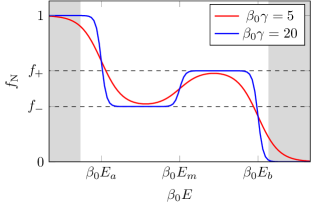
Figure 3: Example of the nonequilibrium distribution given in Eq. (28), with $\beta_{0}E_{a}=-2$, $\beta_{0}E_{b}=1$, $E_{m}=(E_{a}+E_{b})/2$, and two different values of the sharpness $\gamma$. The dashed horizontal lines indicate the values $f_{+}\approx 0.62$ and $f_{-}=1-f_{+}\approx 0.38$, cf. Eq. (27). The non-shaded region corresponds to the selected energy interval with $\Delta=5$. Energies are taken with respect to a common chemical potential $\mu=0$ and a reference temperature $T_{0}.$

Moreover, we choose the interface transparency, $\tau_{\mathrm{int}}(E)$, in such a way that all the energy integrals are limited to the interval $(E_{a}-|E_{a}|/\Delta,E_{b}+|E_{b}|/\Delta)$, thus keeping energy regions where the nonequilibrium distribution can deviate significantly from the optimal values $f_{\pm}$ (see non-shaded region in Fig. 3 for an example). Having fixed the integration interval, one can calculate all the transport quantities. In particular, the demon conditions $I_{\text{N}}=I^{\mathrm{E}}_{\mathrm{N}}=0$ will be used to fix the values of $E_{a}$ and $E_{b}$.

Focusing on the classical part of the resource fluctuations, for which inequality (14) holds, we now study the behavior of the ratio

$$\mathcal{R}^{3\mathrm{T}}_{\text{cl}}=\frac{S_{\mathrm{NN,cl}}^{\Sigma}{+}\frac{k_{\text{B}}^{2}}{4}S_{\mathrm{NN,cl}}}{2k_{\text{B}}|I^{\Sigma}_{\mathrm{N}}|}\geq 1,$$ (30)

as a function of the transition sharpness $\gamma$ and the parameter $\Delta$ governing how much the allowed energy interval exceeds the boundaries $E_{a}$ and $E_{b}$.

The result is shown in Fig. 4. The dark blue region represents the parameter space where the ratio $\mathcal{R}^{3\mathrm{T}}_{\text{cl}}$ is relatively low (the global minimum in the displayed plot is around 3.5). The behavior in Fig. 4 can be roughly understood as follows. Inequality (11a) tells us that the bound can be approached when $f_{\text{N}}$ is close to the optimal values $f_{\pm}$. By contrast, if $f_{\text{N}}$ approaches the values 0 or 1, the inequality becomes very inaccurate. Therefore, to achieve a small $\mathcal{R}^{3\mathrm{T}}_{\text{cl}}$ the contributions where $f_{\text{N}}\approx 0,1$ need to be suppressed while maintaining the ones where $f_{\text{N}}\approx f_{\pm}$. As depicted in Fig. 4, this can be achieved in two ways. For large $\Delta$ and large $\gamma$ the regions where $f_{\text{N}}$ is not close to $f_{\pm}$ are filtered out: a large value of $\gamma$ makes $f_{\text{N}}$ transition abruptly between the values 0, $f_{+}$, $f_{-}$, 1 (see the blue line in Fig. 3), and a large value of $\Delta$ selects the energy region where $f_{\text{N}}=f_{+},f_{-}$ as integration interval. This explains the dark blue region in the upper right corners of the plots in Fig. 4.

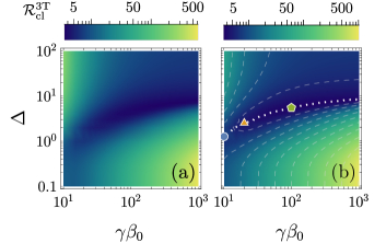
Figure 4: Ratio $\mathcal{R}^{3\mathrm{T}}_{\text{cl}}$ defined in Eq. (30), calculated for the nonequilibrium distribution (28) with $E_{m}=(E_{a}+E_{b})/2$ and $E_{a}$, $E_{b}$ fixed by the demon conditions. The ratio is plotted as a function of the parameters $\gamma$ and $\Delta$. The other parameters are chosen having in mind a refrigerator configuration. Therefore, we set the reference temperature $T_{1}=T_{0}$, a common electrochemical potential $\mu_{1}=\mu_{2}\equiv 0$, and (a) $T_{2}=0.3T_{0}$, (b) $T_{2}=0.5T_{0}$. The markers in (b) indicate the points we use to calculate the cooling power of an N-demon using such a nonequilibrium distribution, see Fig. 5. These points are chosen along the line (white dashed) where $\mathcal{R}^{3\mathrm{T}}_{\text{cl}}$ takes the minimal values as a function of $\gamma$ and $\Delta$.

But one can also achieve a small $\mathcal{R}^{3\mathrm{T}}_{\text{cl}}$ value by decreasing the parameters $\Delta$ and $\gamma$, visible on the diagonals of both panels of Fig. 4. Decreasing $\gamma$, the steps in $f_{\text{N}}$ become smoother, see the red line in Fig. 3, meaning that $f_{\mathrm{N}}$ deviates only slightly from the optimal values $f_{\pm}$ in extended energy intervals. Indeed, Fig. 2(a) shows that for smooth distribution functions (arising from large temperatures in Fig. 2(a)) the region where the ratio $|\sigma_{\alpha}|/(\sigma_{\alpha}^{2}+1/4)$ is close to 1 is significantly increased. As a consequence, it is possible to extend the integration interval beyond $[E_{a},E_{b}]$ by decreasing $\Delta$ while staying in a range for which Eq. (11a) is sufficiently accurate. Note that detailed features of Fig. 4 furthermore heavily rely on the interconnection between the different parameters through the demon conditions, and can hence not straightforwardly be explained by the simple reasoning above.

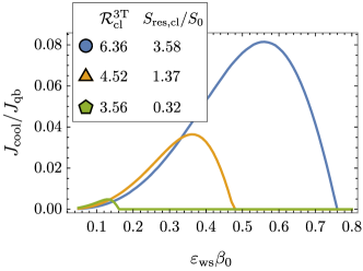
Figure 5: Cooling power $J_{\text{cool}}$ when the three terminal N-demon is operated as a refrigerator, with $T_{1}=T_{0}$, $T_{2}=0.5T_{0}$, and $\mu_{1}=\mu_{2}=0$. The working substance exploits the incoming nonequilibrium distribution (28) by using a filter transmission probability $\tau_{\text{ws}}$ of the form (31). The three curves correspond to different working points, indicated in Fig. 4(b). The associated values of the ratio $\mathcal{R}^{3\mathrm{T}}_{\text{cl}}$ and the classical resource fluctuations $S_{\text{res,cl}}$ (in units of $S_{0}=2k_{\text{B}}^{3}T_{0}/h$) are shown in the legend.

Overall, our analysis shows that it is possible to conceive nonthermal distributions allowing one to approach the bounds derived in the previous section, even when satisfying the demon conditions. It remains to be shown that the N-demon can produce a useful output in these regimes. We illustrate this for the example of the demon acting as a refrigerator cooling contact 2, which is set at temperature $T_{2}<T_{1}$. The working substance must be equipped with an energy-dependent transmission probability $\tau_{\text{ws}}(E)$ to be able to exploit the incoming nonthermal resource. For this purpose, we choose an energy filter in the form of a boxcar function:

$$\tau_{\text{ws}}(E)=\begin{cases}1&-\varepsilon_{\text{ws}}\leq E\leq\varepsilon_{\text{ws}}\,,\\ 0&\text{otherwise}\,.\end{cases}$$ (31)

This choice is motivated by the high relevance of this type of transmission in quantum thermoelectrics Whitney (2014, 2015), also concerning noise Kheradsoud et al. (2019); Timpanaro et al. (2023); Balduque and Sánchez (2023). The results for the cooling power $J_{\text{cool}}=-J_{2}$ obtained in this situation are shown in Fig. 5 as a function of the filter half-width $\varepsilon_{\text{ws}}$. The cooling power is normalized with Pendry’s bound Pendry (1983)

$$J_{\text{qb}}=\frac{\pi^{2}k_{\text{B}}^{2}}{6h}T_{\text{cold}}^{2},$$ (32)

which sets the maximum amount of heat that can be carried away from a contact with a given temperature, here $T_{\mathrm{cold}}$. Quite remarkably, it is possible to have a finite cooling power, approaching almost 10% of Pendry’s bound. Moreover, Fig. 5 also shows that the curve displaying the largest cooling power corresponds to the largest value of $S_{\text{res,cl}}=S_{\text{NN,cl}}^{\Sigma}+\frac{k_{\text{B}}^{2}}{4}S_{\text{NN,cl}}$. This means that for the example considered here, the classical resource fluctuations grow faster than the entropy production of the N-terminal and the entropy reduction in the working substance—more than imposed by the inequality (14).

V Noise bounds for an engineered multi-terminal N-demon

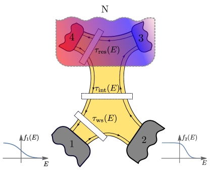
Figure 6: A four-terminal configuration for the N-demon, where the nonthermal resource is implemented by a coherent conductor mixing the occupation probabilities of two equilibrium contacts, 3 and 4, thanks to an energy-dependent transmission function $\tau_{\text{res}}(E)$ associated with a scatterer in the resource region.

Until now, we have considered a device where the resource is a single terminal providing a given nonthermal distribution $f_{\text{N}}$ and we have purposefully not introduced a specific mechanism creating this distribution. Nonthermal distributions are ubiquitous in nanoscale devices and various examples have been analyzed how to engineer them, such as with squeezed states Roßnagel et al. (2014); Correa et al. (2014); Abah and Lutz (2014); Manzano et al. (2016); Agarwalla et al. (2017); Manzano (2018), quantum correlations Francica et al. (2017), or driven contacts Ryu et al. (2022).

To give a concrete, but simple example, representative of a system in contact with different environments, yet realizable and tunable in experiment, we analyze in the following the setup shown in Fig. 6. Here, the resource consists of a set of two thermal contacts, which can have different temperatures and electrochemical potentials, connected via a coherent conductor characterized by an energy-dependent scatterer, with transmission probability $\tau_{\text{res}}(E)$. This combination of different thermal contacts is an extremely simple way to engineer an effective nonthermal distribution, namely

$$f_{\text{N}}(E)=\tau_{\text{res}}(E)f_{4}(E)+[1-\tau_{\text{res}}(E)]f_{3}(E)\,.$$ (33)

Such a configuration, as previously studied in Refs. Sánchez et al. (2019); Hajiloo et al. (2020), is expected to be experimentally realizable while being highly tunable. Indeed, nanofabrication techniques in two-dimensional electron gases allow for the realization of complex energy-filtering setups in the quantum Hall regime Altimiras et al. (2010). In addition, the parameters of the transmission function $\tau_{\text{res}}(E)$ can usually be controlled by means of gate voltages, as in the case of a quantum point contact Büttiker (1990) or resonant quantum-dot-like structures Altimiras et al. (2010); Gasparinetti et al. (2011, 2012). The resource region can hence be engineered such that it constitutes the “demon” part of the setup, providing a nonthermal resource at vanishing average charge and energy currents out of the shaded region in Fig. 6 and into the working substance. Note that distributions analogous to Eq. (33) can also arise in conductors coupled to different baths and subject to different equilibration/thermalization processes, as demonstrated in Ref. Tesser et al. (2023a) for a hot-carrier solar cell.

V.1 General noise bounds for the multi-terminal resource

We now analyze how the entropy production in the resource (and hence the entropy reduction in the working substance) is bounded by the fluctuations occurring in the resource terminals. We therefore exploit the previously presented bound (III), but now consider the sum of the contributions from the two thermal contacts that together constitute the demon part of the device. Indeed, using Eq. (III), we get

$$S_{33,\text{cl}}^{\Sigma}+S_{44,\text{cl}}^{\Sigma}+\frac{k_{\text{B}}^{2}}{4}[S_{33,\text{cl}}+S_{44,\text{cl}}]\geq 2k_{\text{B}}(|I^{\Sigma}_{3}|+|I^{\Sigma}_{4}|).$$ (34)

Note that in this inequality, the sum of the moduli of the entropy productions in the resource terminals appears. If—as desired—the two resource terminals indeed produce entropy, this sum equals the total entropy production in the resource. Otherwise, we have $|I^{\Sigma}_{3}|+|I^{\Sigma}_{4}|\geq|I^{\Sigma}_{3}+I^{\Sigma}_{4}|\geq|I^{\Sigma}_{1}+I^{\Sigma}_{2}|$, the latter being the entropy reduction in the working substance. As a side remark, note that the total entropy production of a nonthermal distribution arising from a coherent mixing as presented here is always larger than the entropy production $I^{\Sigma}_{\text{N}}$ of a single terminal with an analogous distribution function $f_{\mathrm{N}}$, see Ref. Tesser et al. (2023a).

Recalling that terminals 3 and 4 are in a thermal state, the entropy fluctuations reduce to the heat noise $S_{\alpha\alpha}^{J}$, such that

$$S_{\text{res,cl}}^{\mathrm{4T}} \equiv \frac{S_{33,\text{cl}}^{J}}{T_{3}^{2}}+\frac{S_{44,\text{cl}}^{J}}{T_{4}^{2}}+\frac{k_{\text{B}}^{2}}{4}\left(S_{33,\text{cl}}+S_{44,\text{cl}}\right)$$ (35)

$$\geq -2k_{\text{B}}I^{\Sigma}_{\text{ws}}.$$

This relation provides us with a relevant definition of classical resource fluctuations of the 4-terminal setup, $S_{\text{res,cl}}^{\mathrm{4T}}$, that will be used for the device characterization. This inequality is extended to the full noise, including quantum contributions, by exploiting Eq. (20), yielding

$$S_{\text{res}}^{\mathrm{4T}} \equiv \left[\frac{S_{33}^{J}}{T_{3}^{2}}+\frac{k_{\text{B}}^{2}}{4}S_{33}\right]+\left[\frac{S_{44}^{J}}{T_{4}^{2}}+\frac{k_{\text{B}}^{2}}{4}S_{44}\right]$$ (36)

$$\geq -2\inf\{|s_{33}(E)|^{2},|s_{44}(E)|^{2}\}k_{\text{B}}I^{\Sigma}_{\text{ws}}.$$

In the following Section V.2, we analyze how the entropy production and its fluctuations behave in concrete realizations of engines and refrigerators realized in quantum-Hall conductors with a set of two terminals, together acting as a demonic nonthermal resource (without average charge and heat currents into the working substance).

V.2 Analysis of specific device realizations

Here, we characterize the performance of the device in Fig. 6 with respect to the bounds we have previously derived. We consider both a refrigerator and an engine configuration. In all cases, we choose to fulfill the demon conditions (7) by adjusting the chemical potentials $\mu_{3}$ and $\mu_{4}$ of the resource region. The free parameters of the resource region are thus the temperatures $T_{3}$ and $T_{4}$, as well as the transmission function $\tau_{\text{res}}$. We furthermore consider here $\tau_{\text{int}}=1$, whereas $\tau_{\text{ws}}$ and $\tau_{\text{res}}$ are both chosen to be sharp step functions, which can be obtained as a limiting case of a QPC transmission van Wees et al. (1988); Büttiker (1990); van Houten et al. (1992); Kheradsoud et al. (2019)

$$\tau_{\text{QPC}}(E)=\frac{1}{1+\exp[-2\pi\gamma_{\mathrm{QPC}}(E-\epsilon)]}\,,$$ (37)

with $\gamma_{\mathrm{QPC}}$ larger than all relevant energy scales (temperatures, biases) in the system. We address two types of engine operation: In Fig. 7, we analyze the system working as a refrigerator, where the working substance is characterized by $T_{2}<T_{1}$ and $\mu_{1}=\mu_{2}=0$. The nonthermal resource is exploited to obtain a finite cooling power in the resource, namely a heat current flowing out of the cold contact 2 and into the hotter contact 1. In Fig. 8, we analyze the system working as an engine producing electrical power, where the working substance is characterized by $T_{1}=T_{2}$. Power is produced by driving a particle current against the potential difference $\mu_{1}-\mu_{2}$.

In these figures, we plot in panels (a) the desired output, namely the cooling power and the produced electrical power. We also plot the classical resource fluctuations, i.e., the combination of classical entropy and particle current fluctuations as defined by Eq. (35), in panels (b). Furthermore, we show the sum of the moduli of the entropy production in the two resource terminals (ideally corresponding to the total entropy production in the resource), namely $|I^{\Sigma}_{3}|+|I^{\Sigma}_{4}|$, in panels (c). Finally, in panels (d) of Figs. 7 and 8, we plot the ratios between resource fluctuations and entropy production. We compare the following ratios

$$\mathcal{R}_{\text{cl}}^{\text{4T}}=\frac{1}{2k_{\text{B}}}\frac{S_{\text{res,cl}}^{\text{4T}}}{|I^{\Sigma}_{3}|+|I^{\Sigma}_{4}|},$$ (38a)

$$\mathcal{R}^{\text{4T}}=\frac{1}{2k_{\text{B}}}\frac{S_{\text{res}}^{\text{4T}}}{|I^{\Sigma}_{3}|+|I^{\Sigma}_{4}|},$$ (38b)

$$\mathcal{R}_{\text{NN}}^{\text{4T}}=\frac{1}{2k_{\text{B}}}\frac{S_{\text{res,NN}}^{\text{4T}}}{|I^{\Sigma}_{3}|+|I^{\Sigma}_{4}|}.$$ (38c)

For the first ratio, we know from Eq. (34) that $\mathcal{R}_{\text{cl}}^{\text{4T}}\geq 1$. By contrast, the second ratio involving the full resource fluctuations, can become smaller than 1 due to the quantum noise contribution, which can be negative. Indeed, in the considered setup, where $|s_{33}(E)|^{2},|s_{44}(E)|^{2}$ can become zero, the inequality (36) is uninformative, only requiring the trivial fact that the total noise is positive, i.e., $\mathcal{R}^{\text{4T}}\geq 0$. We compare these two ratios to a third one, involving the full fluctuations of the zero-average currents flowing from the two-terminal resource into the working substance, $\hat{I}_{\text{N}}=\hat{I}_{3}+\hat{I}_{4}$ and $\hat{I}_{\text{N}}^{\mathrm{E}}=\hat{I}_{3}^{\mathrm{E}}+\hat{I}_{4}^{\mathrm{E}}$. The fluctuations appearing in Eq. (38c), given by the combination $S_{\text{res,NN}}^{\text{4T}}\equiv S_{\text{NN}}^{\text{4T},\Sigma}+k_{\text{B}}^{2}S_{\text{NN}}^{\text{4T}}/4$, hence also contain the cross-correlation terms between currents $\hat{I}_{3}^{X}$ and $\hat{I}_{4}^{X}$, namely $S_{\text{NN}}^{\text{4T},X}\equiv S_{33}^{X}+S_{44}^{X}+S_{43}^{X}+S_{34}^{X}$. This is one further possibility to quantify the fluctuations related to the nonthermal resource. Note however, that while being an experimentally relevant quantity, it does not unambiguously quantify the fluctuations of a generic nonthermal resource described by the distribution function $f_{\mathrm{N}}$, as it might seem.

Indeed, while the average particle and energy currents $I_{\text{N}}$ and $I_{\text{N}}^{\mathrm{E}}$ flowing from the two-terminal resource considered in this section correspond to the average currents flowing from a single nonthermal resource with an equivalent distribution $f_{\text{N}}$ in Eq. (33), see Eq. (23), the noise of the 4-terminal system

$$\begin{split}S_{\text{NN}}^{\text{4T,E}}=\frac{2}{h}\int dE\,&E^{2}\tau_{\text{int}}[F_{22}+(1-\tau_{\text{res}})F_{33}+\tau_{\text{res}}F_{44}\\ &+(1-\tau_{\text{int}})(1-\tau_{\text{res}})(f_{2}-f_{3})^{2}\\ &+\tau_{\text{res}}(1-\tau_{\text{int}})(f_{2}-f_{4})^{2}\\ &+\tau_{\text{int}}\tau_{\text{res}}(1-\tau_{\text{res}})(f_{3}-f_{4})^{2}],\end{split}$$ (39)

is generally different from the one of the 3-terminal system $S_{\text{NN}}^{\mathrm{E}}$ in Eq. (26) (and equivalently for the particle current noise). The reason for this is that the noise is nonlinear. Hence, the fluctuations of the effective N-terminal $S_{\text{res,NN}}^{\text{4T}}$ do not generally satisfy the bound in Eq. (36), as demonstrated in Appendix B.

In the following, we discuss the described quantities for the realization of the N-demon for refrigeration and power production.

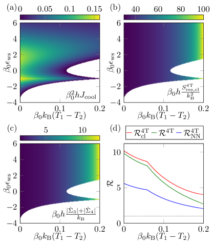
Figure 7: Results for a refrigerator configuration where both $\tau_{\text{ws}}$ and $\tau_{\text{res}}$ are sharp step functions, see Eq. (37). (a) Cooling power, (b) classical resource fluctuations $S_{\text{res,cl}}$, and (c) entropy production $|I^{\Sigma}_{3}|+|I^{\Sigma}_{4}|$ as a function of $\Delta T=T_{1}-T_{2}$ and of the position $\epsilon_{\text{ws}}$ of the step function onset in the working substance. (d) Ratio between the classical resource fluctuations, classical and quantum resource fluctuations, and fluctuations of the effective N-terminal and the entropy production $2k_{\text{B}}(|I^{\Sigma}_{3}|+|I^{\Sigma}_{4}|)$. The plotted ratios are independent of $\epsilon_{\text{ws}}$. In all panels, we set $\mu_{1}=\mu_{2}=0$, $T_{1}=T_{0}$, $T_{3}=T_{4}=1.2T_{0}$, and $\beta_{0}\epsilon_{\text{res}}=-1$. The white regions in the density plots are those where no cooling is possible under demon conditions.

V.2.1 N-demon for cooling

We start by presenting results for the N-demon operating as a refrigerator. Here, we exploit the nonthermal resource to cool contact 2 in the working substance. The results are presented in Fig. 7. We first notice that it is possible to obtain a finite cooling power even when the temperatures of the resource contacts are higher than the temperatures in the working substance, here for $T_{1}=T_{0}$, $0.8T_{0}<T_{2}<T_{0}$, and $T_{3}=T_{4}=1.2T_{0}$. In contrast to absorption refrigerators, where refrigeration is driven by a hot contact Segal (2018); Mitchison and Potts (2019); Manikandan et al. (2020), this however does not lead to any energy exchange on average between resource and working substance in the situation studied here. In Fig. 7(a), we find two maxima in the cooling power $J_{\mathrm{cool}}$ as function of $\epsilon_{\mathrm{ws}}$. One of them is found at $\epsilon_{\mathrm{ws}}=\epsilon_{\mathrm{res}}=-k_{\mathrm{B}}T_{0}$, where the filtering in the resource region and in the working substance takes place at the same energy. The other one is situated around $\epsilon_{\mathrm{ws}}\approx 2k_{\mathrm{B}}T_{0}$; which of the two features is the global maximum depends on the temperature difference in the working substance and changes approximately at the place where the entropy production in contact 3 is found to change sign, see also discussion of panel (d).

The classical resource fluctuations, $S_{\text{res,cl}}^{\text{4T}}$, in panel (b), and the entropy production, $|I^{\Sigma}_{3}|+|I^{\Sigma}_{4}|$, in panel (c), show similar features: they are both increasing with the temperature bias $T_{1}-T_{2}$ and are independent of the working substance transmission, here parametrized through $\epsilon_{\text{ws}}$. This independence of the working-substance implementation is an important difference compared to standard Maxwell demons, where the entropy production of the demon is typically directly related to the entropy reduction in the working substance, see also Ref. Sánchez et al. (2019). We compare the fluctuations and the entropy production in the resource region through the ratios in Eq. (38) in panel (d). As $\mathcal{R}_{\text{cl}}^{\text{4T}}$, $\mathcal{R}^{\text{4T}}$, $\mathcal{R}_{\text{NN}}^{\text{4T}}$ each characterize the resource region, they are independent of $\epsilon_{\text{ws}}$ in the considered setup, see Fig. 6. First, we notice that the ratio $\mathcal{R}_{\text{cl}}^{\text{4T}}\geq 1$ as required by the inequality (34). Furthermore, panel (d) shows that $\mathcal{R}_{\text{cl}}^{\text{4T}}\geq\mathcal{R}^{\text{4T}}$, which is consistent with the quantum noise contribution being negative. Moreover, we also observe that $\mathcal{R}^{\text{4T}}\geq\mathcal{R}_{\text{NN}}^{\text{4T}}$. While this may in principle be not true (due to the possibility that heat current cross-correlations are positive even for fermionic systems), it turns out to be the case in the analyzed setup. Interestingly, each ratio lies above 1, indicated by the dotted line, which is neither required for the total resource fluctuations, $S_{\text{res}}^{4\mathrm{T}}$, by the inequalities (36), nor for the effective N-terminal fluctuations, $S_{\mathrm{res,NN}}^{4\mathrm{T}}$, by relation (34) together with Eq. (43). Nonetheless, this feature can be attributed to the fact that, while the considered setup has a resource fluctuations-to-entropy-production ratio that is of the order of one, it is still far from being optimal with respect to the bound Eq. (35). The smaller the colder temperature gets (hence with increasing $T_{1}-T_{2}$), the more the ratios approach 1. This is in agreement with the results presented in Fig. 5, where the close-to-optimal values of $\mathcal{R}$ are reached for small cooling powers. By contrast, the ratios decrease with increasing absolute values of the resource fluctuations and the entropy production, which was not the case in the example discussed in Sec. IV.2. Finally, we find a non-differentiable point in the three ratios as function of the temperature difference. This is due to a change of sign in $I^{\Sigma}_{3}$ (from negative to positive), and happens at a temperature close to the temperature at which the global maximum of $J_{\text{cool}}$ changes.

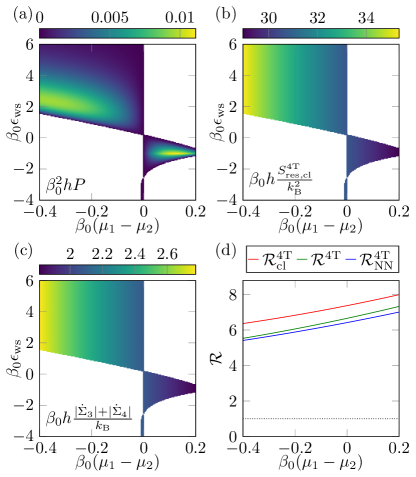
Figure 8: Results for an engine configuration producing electrical power where both $\tau_{\text{ws}}$ and $\tau_{\text{res}}$ are sharp step functions, see Eq (37). (a) Power, (b) classical resource fluctuations $S_{\text{in,cl}}$, and (c) entropy production $|I^{\Sigma}_{3}|+|I^{\Sigma}_{4}|$ as a function of $\Delta T=T_{1}-T_{2}$ and of the position $\epsilon_{\text{ws}}$ of the step function onset in the working substance. (d) Ratio between the classical resource fluctuations, classical and quantum resource fluctuations, and fluctuations of the effective N-terminal and the entropy production $2k_{\text{B}}(|I^{\Sigma}_{3}|+|I^{\Sigma}_{4}|)$. The plotted ratios are independent of $\epsilon_{\text{ws}}$. In all panels, we set $T_{1}=T_{2}=T_{0}$, $T_{3}=T_{4}=0.7T_{0}$, and $\beta_{0}\epsilon_{\text{res}}=-1$ . The white regions in the density plots are those where no power is produced under demon conditions.

V.2.2 N-demon for power production

We now analyze the N-demon operating as an engine, with $T_{2}=T_{1}$ and $\mu_{1}\neq\mu_{2}$ producing electrical power in the working substance, by driving a current against the potential bias. While many of the results that we find are analogous to the results of the refrigerator setup, we here point out relevant differences.

We first of all remark that the parameter regimes in which the demon conditions are fulfilled while useful work is performed in the working substance, are more restricted with respect to the refrigerator setup of the previous subsection, leading to the different shape of the density plot in Fig. 8. This is not a general statement—see also Ref. Hajiloo et al. (2020)—but is a consequence of the complex interplay among the system parameters fixed by the demon conditions, which are influenced by the other freely chosen parameters in the specific setting. Also, the specific implementation chosen here leads to a relatively low output power. We again find two different operational points where the output power has a local maximum, shown as bright spots in Fig. 8(a). We note that the sensitivity of resource fluctuations and entropy production, but also of their ratio, on the potential bias is less pronounced than the temperature-bias dependent case discussed for the refrigerator before.

An interesting observation can be made here concerning the behavior of the output power as compared to the resource fluctuations, the entropy production and their ratios. While in the case discussed in Sec. IV.2 both ratio and resource fluctuations increase with the increase of the maximum cooling power, in the four-terminal refrigerator realization of Fig. 7 the ratio increases whereas the resource fluctuation decrease with the increase of $\max{(J_{\text{cool}})}$. Here, by contrast, we have both features: for positive biases the ratio increases while the resource fluctuations decrease as the maximum power increases, whereas at negative biases the opposite happens. These scenarios are all in line with the bounds on entropy production with respect to resource fluctuations developed in this paper, but they clearly show that the efficiency (namely the ratio between useful output power in the working substance and entropy production in the resource) of the setup does not correlate with the resource fluctuations. The open question under which conditions the output (or the efficiency Hajiloo et al. (2020)) can be optimized given a certain amount of fluctuations is a motivation for future studies relating our findings to generalized thermodynamics uncertainty relations, see also Eq. (15).

VI Conclusions and outlook

In this work, we have analyzed the role of fluctuations in electronic mesoscopic engines powered by nonthermal resources. The key result, Eq. (1), is that whenever a given performance goal in the working substance is set, a minimum amount of particle and local entropy fluctuations in the resource is required. Conversely, a given amount of resource fluctuations sets an upper bound on the useful work that can be done in the system. Interestingly, we find that this bound is set by the classical part of the fluctuations only: When quantum fluctuations are present the noise in the resource part of the system can be lowered, as shown by Eq. (19). Based on the inequality (1), we have introduced a notion of resource fluctuations which we have used to characterize different implementations of N-demons. Considering both the case when the resource is provided by a single contact with a nonthermal occupation probability (Sec. IV.2) and the case of a multi-terminal resource effectively implementing a nonthermal input distribution (Sec. V.1 and V.2), we have shown that the bound imposed by the derived inequalities can be closely approached even when the cooling power or the produced electrical power are finite and the demon conditions (imposing no average particle and energy exchange between resource region and working substance) are fulfilled. The bounds developed in this work provide a general statement on the requirement on fluctuations of an engine resource.

How these predictions can be more closely connected to the currently broadly studied thermodynamic uncertainty relations, as alluded to in Secs. III and V, will be an interesting topic of future research. This is expected to give even further insights into the operation of nonthermal machines.

Appendix A Fluctuating particle, energy, and entropy currents

Using the short-hand notation $\hat{b}_{\alpha}^{\prime}\equiv\hat{b}_{\alpha}(E^{\prime})$ and dropping the energy arguments, we first define for reference the fluctuating particle- and energy-current operators Blanter and Büttiker (2000); Moskalets (2011); Butcher (1990),

$${\hat{I}^{X}_{\alpha}\equiv\int\frac{dEdE^{\prime}}{h}e^{-\frac{i(E-E^{\prime})t}{h}}x_{\alpha}\Big{(}\hat{b}_{\alpha}^{\prime\dagger}\hat{b}_{\alpha}-\hat{a}_{\alpha}^{\prime\dagger}\hat{a}_{\alpha}\Big{)}}$$ (40)

where $\hat{a}_{\alpha}$ and $\hat{b}_{\alpha}$ are the field operators of electrons flowing out of and into contact $\alpha$, respectively. The operators $\hat{b}_{\alpha}^{\prime\dagger}\hat{b}_{\alpha}-\hat{a}_{\alpha}^{\prime\dagger}\hat{a}_{\alpha}$ describe the rate of change of the contact’s occupation $f_{\alpha}$, while providing a probabilistic nature through the random tunnelings of electrons. The factor $x_{\alpha}$, as defined in the main text, determines the transported quantity at every energy, namely $e$ or $E$ for particle and energy current.

Next, we here also introduce the entropy flow into contact $\alpha$ as

$$\begin{split}\hat{I}^{\Sigma}_{\alpha}&\equiv-k_{\text{B}}\int\frac{dEdE^{\prime}}{h}e^{-\frac{i(E-E^{\prime})t}{h}}\Big{[}\Big{(}\hat{b}_{\alpha}^{\prime\dagger}\hat{b}_{\alpha}-\hat{a}_{\alpha}^{\prime\dagger}\hat{a}_{\alpha}\Big{)}\log f_{\alpha}+\\ &\qquad\qquad+\Big{(}\hat{b}_{\alpha}^{\prime}\hat{b}_{\alpha}^{\dagger}-\hat{a}_{\alpha}^{\prime}\hat{a}_{\alpha}^{\dagger}\Big{)}\log(1-f_{\alpha})\Big{]}.\end{split}$$ (41)

The function $f_{\alpha}$ describes the occupation number in contact $\alpha$, i.e. $\langle\hat{a}_{\alpha}^{\prime\dagger}\hat{a}_{\alpha}\rangle=\delta(E-E^{\prime})f_{\alpha}$. Crucially, transport does not affect the occupation of the contact because the latter is considered to be a large bath or, alternatively, its distribution is kept constant by an external agent. The formulation of Eq. (41) relies on concepts borrowed from information theory. In particular, the Shannon information (or surprisal) associated with an event occurring with probability $p$ is given by $-\log p$. From this, one obtains the Shannon entropy, which is the expected value of the information. For the electronic system we are considering here, a channel originating from contact $\alpha$ can be either occupied (with probability $f_{\alpha}$) or empty, with probability $(1-f_{\alpha})$. So, this defines the two possible outcomes of the event “electron being present in the channel”, yielding information $-\log(f_{\alpha})$ and $-\log(1-f_{\alpha})$, respectively. Correspondingly, one can define the information change associated with these outcomes as in Eq. (41), where the information is combined with the rate of change of the reservoir occupation, described via the operator difference $\hat{b}^{\dagger}_{\alpha}\hat{b}_{\alpha}-\hat{a}^{\dagger}_{\alpha}\hat{a}_{\alpha}$. Equipped with these definitions, one can find the entropy change as the expectation value of the information change, $I^{\Sigma}_{\alpha}=\braket{\hat{I}^{\Sigma}_{\alpha}}$, reproducing the expression for the average entropy in the main text, namely Eq. (3), with the prescription (5). Similarly, one can obtain the entropy fluctuations of Eq. (9).

Importantly, this formulation of the information flow relies on the fact that the particles considered here are fermions. Hence, the only considered occupations are zero or one.

Appendix B Current fluctuations in an engineered N-demon

We consider a nonthermal resource consisting of a set of thermal contacts connected through a coherent conductor, see Fig. 6. However, instead of considering the contributing contacts separately—as done in the main text in Eq. (34)—we here consider the total (entropy) currents flowing out of the resource region as well as their fluctuations. We show in this appendix that the bound between entropy currents and their fluctuations is modified due to cross-correlations between currents into the different resource contacts.

B.1 Generic multi-terminal setup

We consider the classical fluctuations of a generic current $\hat{I}^{X}_{\text{N}}=\sum_{\alpha\in\mathfrak{N}}\hat{I}^{X}_{\alpha}$, where $\mathfrak{N}$ is a collection of contacts, defining the resource part of the system. The fluctuations of interest in this multi-terminal resource are given by the combination of correlators $S_{\text{NN,cl}}^{\mathrm{multi},X}=\sum_{\alpha\beta\in\mathfrak{N}}S_{\alpha\beta,\text{cl}}^{X}$. From Eq (9), we write it as

$$\begin{split}S_{\text{NN,cl}}^{\mathrm{multi},X}&=\frac{2}{h}\int dE\sum_{\alpha\beta\in\mathfrak{N}}x_{\alpha}x_{\beta}\Big{[}-F_{\alpha\alpha}|s_{\beta\alpha}|^{2}-F_{\beta\beta}|s_{\beta\alpha}|^{2}+\delta_{\alpha\beta}\sum_{\gamma}|s_{\alpha\gamma}|^{2}(F_{\alpha\gamma}+F_{\gamma\alpha})\Big{]}\\ &=\frac{2}{h}\int dE\left[\sum_{\begin{subarray}{c}\alpha\beta\in\mathfrak{N},\\ \alpha\neq\beta\end{subarray}}x_{\alpha}x_{\beta}\Big{(}-F_{\alpha\alpha}|s_{\beta\alpha}|^{2}-F_{\beta\beta}|s_{\alpha\beta}|^{2}\Big{)}+\sum_{\alpha\in\mathfrak{N}}x_{\alpha}^{2}\sum_{\gamma\neq\alpha}|s_{\alpha\gamma}|^{2}(F_{\alpha\gamma}+F_{\gamma\alpha})\right],\end{split}$$ (42)

where, as in the main text, $x_{\alpha}$ is the weight associated to the current, specifically, $x_{\alpha}=1$ for the particle current and $x_{\alpha}=k_{\text{B}}\sigma_{\alpha}$ for the entropy current. Note that the cross-correlators, $S^{X}_{\alpha\beta,\mathrm{cl}}$ with $\alpha\neq\beta$ that give rise to the first line in Eq. (42), can be either positive or negative depending on the sign of $x_{\alpha}x_{\beta}$. Furthermore, the last line in Eq. (42) has the same structure as Eq. (10a). Therefore, we can use the inequalities (11) to find the following bound

$$\begin{split}S_{\text{NN,cl}}^{\mathrm{multi},\Sigma}+\frac{k_{\text{B}}^{2}}{4}S_{\text{NN,cl}}^{\mathrm{multi}}&\geq\frac{2k_{\text{B}}^{2}}{h}\int dE\Bigg{\{}\sum_{\alpha\in\mathfrak{N}}|\sigma_{\alpha}|\sum_{\gamma\neq\alpha}|s_{\alpha\gamma}|^{2}|f_{\alpha}-f_{\gamma}|+\sum_{\begin{subarray}{c}\alpha\beta\in\mathfrak{N},\\ \alpha\neq\beta\end{subarray}}\left(\sigma_{\alpha}\sigma_{\beta}+\frac{1}{4}\right)\left(-F_{\alpha\alpha}|s_{\beta\alpha}|^{2}-F_{\beta\beta}|s_{\alpha\beta}|^{2}\right)\Bigg{\}}\\ &\geq 2k_{\text{B}}\sum_{\alpha\in\mathfrak{N}}|I^{\Sigma}_{\alpha}|+\frac{2k_{\text{B}}^{2}}{h}\int dE\sum_{\begin{subarray}{c}\alpha\beta\in\mathfrak{N},\\ \alpha\neq\beta\end{subarray}}\left(\sigma_{\alpha}\sigma_{\beta}+\frac{1}{4}\right)\left(-F_{\alpha\alpha}|s_{\beta\alpha}|^{2}-F_{\beta\beta}|s_{\alpha\beta}|^{2}\right).\end{split}$$ (43)

Note that the second term on the right hand side of this inequality, adding up to the sum of absolute values of entropy productions in the separate contacts, can be negative. This means that the bound on the fluctuations in the total current from the engineered nonthermal resource is less restrictive and the fluctuations can be smaller compared to the sum in Eq. (14). Note however, that for the example treated in Sec. V.2 (see Figs. 7 and 8), the fluctuations on the left hand side of Eq. (43) are larger than the entropy production in the right hand side of Eq. (34).

B.2 Linear response of a four-terminal system

We show here that, within linear response, the particle- and energy-current fluctuations of a single nonthermal terminal, see Fig. 1, and the noise of the total particle and energy currents from an engineered nonthermal two-terminal resource, see Fig. 6, are identical. We therefore consider the 4-terminal setup and assume that $(\mu_{\alpha}-\mu_{0})/(k_{\text{B}}T_{0})\ll 1$, $(T_{\alpha}-T_{0})/T_{0}\ll 1$, for some reference temperature $T_{0}$ and chemical potential $\mu_{0}\equiv 0$. Then, we can expand all currents up to linear order in the affinities $\mathcal{A}_{\alpha}^{\mu}=(\mu_{\alpha}-\mu_{0})/(k_{\text{B}}T_{0})$, $\mathcal{A}_{\alpha}^{T}=(T_{\alpha}-T_{0})/(k_{\text{B}}T_{0}^{2})$.

B.2.1 Demon conditions

With this and with the definition $\mathcal{A}_{\alpha\beta}^{\mu,T}\equiv\mathcal{A}_{\alpha}^{\mu,T}-\mathcal{A}_{\beta}^{\mu,T}$, the demon conditions read

$$g_{\text{int}}^{(0)}\mathcal{A}_{23}^{\mu}+g_{\text{int}}^{(1)}\mathcal{A}_{23}^{T}+h_{\text{res}}^{(0)}\mathcal{A}_{34}^{\mu}+h_{\text{res}}^{(1)}\mathcal{A}_{34}^{T} =0$$

$$g_{\text{int}}^{(1)}\mathcal{A}_{23}^{\mu}+g_{\text{int}}^{(2)}\mathcal{A}_{23}^{T}+h_{\text{res}}^{(1)}\mathcal{A}_{34}^{\mu}+h_{\text{res}}^{(2)}\mathcal{A}_{34}^{T} =0$$

where we have defined the integrals

$$g_{i}^{(\nu)} =\int dE\,\tau_{i}(E)\xi(E)E^{\nu}\,,$$ (44)

$$h_{i}^{(\nu)} =\int dE\,\tau_{i}(E)\tau_{\text{int}}(E)\xi(E)E^{\nu}\,,$$ (45)

with $\xi(E)=-k_{\text{B}}T_{0}(\partial f_{0}/\partial E)$. Using these equations to fix the values of the chemical potentials $\mu_{3}$ and $\mu_{4}$, we find

$$\mu_{3} =\mu_{2}+\frac{\beta}{\alpha}\frac{T_{3}-T_{2}}{T_{0}}+\frac{\gamma}{\alpha}\frac{T_{4}-T_{3}}{T_{0}},$$ (46)

$$\mu_{4} =\mu_{2}+\frac{\delta}{\alpha}\frac{T_{3}-T_{2}}{T_{0}}+\frac{\zeta}{\alpha}\frac{T_{4}-T_{3}}{T_{0}},$$ (47)

with the coefficients

$$\alpha =h_{\text{res}}^{(1)}g_{\text{int}}^{(0)}-h_{\text{res}}^{(0)}g_{\text{int}}^{(1)},$$ (48)

$$\beta =h_{\text{res}}^{(0)}g_{\text{int}}^{(2)}-h_{\text{res}}^{(1)}g_{\text{int}}^{(1)},$$ (49)

$$\gamma =h_{\text{res}}^{(2)}h_{\text{res}}^{(0)}-[h_{\text{res}}^{(1)}]^{2},$$ (50)

$$\delta =g_{\text{int}}^{(1)}(g_{\text{int}}^{(1)}-h_{\text{res}}^{(1)})+g_{\text{int}}^{(2)}(h_{\text{res}}^{(0)}-g_{\text{int}}^{(0)}),$$ (51)

$$\zeta =h_{\text{res}}^{(1)}(g_{\text{int}}^{(1)}-h_{\text{res}}^{(1)})+h_{\text{res}}^{(2)}(h_{\text{res}}^{(0)}-g_{\text{int}}^{(0)}).$$ (52)

B.2.2 Fluctuations

All noise contributions can be expanded up to linear order, too. Let us start with the 4-terminal setup and expand the noise (39) at linear order in the affinities. We have

$$f_{\alpha}(1-f_{\alpha})\approx f_{0}(1-f_{0})+\xi(\mathcal{A}_{\alpha}^{\mu}+E\mathcal{A}_{\alpha}^{T})(1-2f_{0}).$$ (53)

All the terms of the form $(f_{\alpha}-f_{\beta})^{2}$ are at least quadratic in the affinities. In particular the quantum part of the noise, Eq. (10b), (or also the shot noise in other ways of dividing noise contributions) at this order vanishes. We are therefore left with

$$S_{\text{NN}}^{\text{4T}} =2r^{(0)}+(\mathcal{A}_{2}^{\mu}+\mathcal{A}_{3}^{\mu})p^{(0)}+(\mathcal{A}_{2}^{T}+\mathcal{A}_{3}^{T})p^{(1)}$$

$$\quad+\mathcal{A}_{43}^{\mu}q^{(0)}+\mathcal{A}_{43}^{T}q^{(1)}$$ (54a)

$$S_{\text{NN}}^{\text{4T,E}} =2r^{(2)}+(\mathcal{A}_{2}^{\mu}+\mathcal{A}_{3}^{\mu})p^{(2)}+(\mathcal{A}_{2}^{T}+\mathcal{A}_{3}^{T})p^{(3)}$$

$$\quad+\mathcal{A}_{43}^{\mu}q^{(2)}+\mathcal{A}_{43}^{T}q^{(3)}$$ (54b)

where

$$r^{(\nu)} =\int dE\,\tau_{\text{int}}(E)f_{0}(E)[1-f_{0}(E)]E^{\nu},$$ (55)

$$p^{(\nu)} =\int dE\,\tau_{\text{int}}(E)\xi(E)[1-2f_{0}(E)]E^{\nu},$$ (56)

$$q^{(\nu)} =\int dE\,\tau_{\text{int}}(E)\tau_{\text{res}}(E)\xi(E)[1-2f_{0}(E)]E^{\nu}.$$ (57)

If we now consider the result in the 3-terminal setup with an effective nonthermal distribution $f_{\text{N}}$ given by Eq. (33), the noise is given by Eq. (26). It contains the term $f_{2}(1-f_{2})$, just as the 4-terminal expression (39), and the terms $f_{\text{N}}(1-f_{\text{N}})$ and $(f_{2}-f_{\text{N}})^{2}$. It is easy to see that the latter does not contribute at linear order in the affinities, while the remainder gives

$$\begin{split}f_{\text{N}}(1-f_{\text{N}})&=f_{3}(1-f_{3})+\tau_{\text{res}}(f_{4}-f_{3})(1-2f_{3})\\ &\quad-\tau_{\text{res}}^{2}(f_{3}-f_{4})\\ &\approx f_{0}(1-f_{0})+\xi(1-2f_{0})(\mathcal{A}_{3}^{\mu}+E\mathcal{A}_{3}^{T})\\ &\quad+\tau_{\text{res}}\xi(1-2f_{0})(\mathcal{A}_{43}^{\mu}+E\mathcal{A}_{43}^{T})\end{split}$$ (58)

which shows that the noise (26) for the 3-terminal N-demon becomes identical to the expression given in Eq. (54) in linear response.

Appendix C Analytical expressions for energy noise with QPC transmissions

Useful analytical expressions for charge and energy currents in the presence of sharp step-function transmissions can be found in Appendix A of Ref. Hajiloo et al. (2020). Here we present some analytical expressions for the noise, in the case when all terminals are described by a thermal distribution, as considered in Sec. V. The calculation of the energy noise [see, e.g., Eq. (39)] involves integrals of the form

$$\mathcal{J}_{\alpha}=\int_{E_{0}}^{+\infty}dEE^{2}f_{\alpha}(E)[1-f_{\alpha}(E)]$$ (59)

where $f_{\alpha}(E)$ is a thermal distribution and $E_{0}$ is the onset energy of a sharp step function transmission $\tau_{\text{QPC}}=\Theta(E-E_{0})$. This integral can be evaluated analytically, yielding

$$\begin{split}\mathcal{J}_{\alpha}&=\mathcal{J}_{\alpha}^{\text{open}}+(k_{\text{B}}T_{\alpha})^{3}\big{[}2x_{\alpha}\log(1+e^{x_{\alpha}-y_{\alpha}})\\ &\quad+2\mathrm{Li}_{2}(-e^{x_{\alpha}-y_{\alpha}})-x_{\alpha}^{2}(1+e^{y_{\alpha}-x_{\alpha}})^{-1}\big{]},\end{split}$$ (60)

where $\text{Li}_{2}$ is the dilogarithm function, $x_{\alpha}=E_{0}/(k_{\text{B}}T_{\alpha})$, $y_{\alpha}=\mu_{\alpha}/(k_{\text{B}}T_{\alpha})$, and

$$\mathcal{J}_{\alpha}^{\text{open}}=(k_{\text{B}}T_{\alpha})^{3}\left[\frac{\pi^{2}}{3}+y_{\alpha}^{2}\right]$$ (61)

is the result for an open channel with $E_{0}\to-\infty$. Integrals involving factors of the form $(f_{\alpha}-f_{\beta})^{2}$ do not have a closed form when the Fermi functions have different temperatures and we resort to a numerical integration to evaluate them.

References

- Binder et al. (2018) F. Binder, L. A. Correa, C. Gogolin, J. Anders, and G. Adesso, eds., Thermodynamics in the Quantum Regime (Springer International Publishing, Cham, Switzerland, 2018).
- Strasberg (2022) P. Strasberg, Quantum Stochastic Thermodynamics (Oxford University Press, Oxford, England, UK, 2022).
- Esposito et al. (2009) M. Esposito, U. Harbola, and S. Mukamel, “Nonequilibrium fluctuations, fluctuation theorems, and counting statistics in quantum systems,” Rev. Mod. Phys. 81, 1665–1702 (2009).
- Seifert (2008) U. Seifert, “Stochastic thermodynamics: principles and perspectives,” Eur. Phys. J. B 64, 423–431 (2008).
- Benenti et al. (2017) G. Benenti, G. Casati, K. Saito, and R. S. Whitney, “Fundamental aspects of steady-state conversion of heat to work at the nanoscale,” Phys. Rep. 694, 1–124 (2017).
- Scully et al. (2003) M. O. Scully, M. S. Zubairy, G. S. Agarwal, and H. Walther, “Extracting Work from a Single Heat Bath via Vanishing Quantum Coherence,” Science 299, 862–864 (2003).
- Francica et al. (2017) G. Francica, J. Goold, F. Plastina, and M. Paternostro, “Daemonic ergotropy: enhanced work extraction from quantum correlations,” npj Quantum Inf. 3, 1–6 (2017).
- Niedenzu et al. (2018) W. Niedenzu, V. Mukherjee, A. Ghosh, A. G. Kofman, and G. Kurizki, “Quantum engine efficiency bound beyond the second law of thermodynamics,” Nat. Commun. 9, 1–13 (2018).
- Ghosh et al. (2019) A. Ghosh, V. Mukherjee, W. Niedenzu, and G. Kurizki, “Are quantum thermodynamic machines better than their classical counterparts?” Eur. Phys. J. Spec. Top. 227, 2043–2051 (2019).
- Bennett (1982) C. H. Bennett, “The thermodynamics of computation—a review,” Int. J. Theor. Phys. 21, 905–940 (1982).
- Bérut et al. (2012) A. Bérut, A. Arakelyan, A. Petrosyan, S. Ciliberto, R. Dillenschneider, and E. Lutz, “Experimental verification of Landauer’s principle linking information and thermodynamics,” Nature 483, 187–189 (2012).
- Parrondo et al. (2015) J. M. R. Parrondo, J. M. Horowitz, and T. Sagawa, “Thermodynamics of information,” Nat. Phys. 11, 131–139 (2015).
- Krishnamurthy et al. (2016) S. Krishnamurthy, S. Ghosh, D. Chatterji, R. Ganapathy, and A. K. Sood, “A micrometre-sized heat engine operating between bacterial reservoirs,” Nat. Phys. 12, 1134–1138 (2016).
- Holubec et al. (2020) V. Holubec, S. Steffenoni, G. Falasco, and K. Kroy, “Active Brownian heat engines,” Phys. Rev. Res. 2, 043262 (2020).
- Pietzonka et al. (2019) P. Pietzonka, É. Fodor, C. Lohrmann, M. E. Cates, and U. Seifert, “Autonomous Engines Driven by Active Matter: Energetics and Design Principles,” Phys. Rev. X 9, 041032 (2019).
- Abah and Lutz (2014) O. Abah and E. Lutz, “Efficiency of heat engines coupled to nonequilibrium reservoirs,” Europhys. Lett. 106, 20001 (2014).
- Tesser et al. (2023a) L. Tesser, R. S. Whitney, and J. Splettstoesser, “Thermodynamic Performance of Hot-Carrier Solar Cells: A Quantum Transport Model,” Phys. Rev. Appl. 19, 044038 (2023a).
- Strasberg et al. (2017) P. Strasberg, G. Schaller, T. Brandes, and M. Esposito, “Quantum and Information Thermodynamics: A Unifying Framework Based on Repeated Interactions,” Phys. Rev. X 7, 021003 (2017).
- Konopik et al. (2020) M. Konopik, A. Friedenberger, N. Kiesel, and E. Lutz, “Nonequilibrium information erasure below kTln2,” Europhys. Lett. 131, 60004 (2020).
- Ryu et al. (2022) S. Ryu, R. López, L. Serra, and D. Sánchez, “Beating Carnot efficiency with periodically driven chiral conductors,” Nat. Commun. 13, 1–6 (2022).
- Whitney et al. (2016) R. S. Whitney, R. Sánchez, F. Haupt, and J. Splettstoesser, “Thermoelectricity without absorbing energy from the heat sources,” Physica E 75, 257–265 (2016).
- Sánchez et al. (2019) R. Sánchez, J. Splettstoesser, and R. S. Whitney, “Nonequilibrium System as a Demon,” Phys. Rev. Lett. 123, 216801 (2019).
- Esposito and Schaller (2012) M. Esposito and G. Schaller, “Stochastic thermodynamics for “Maxwell demon” feedbacks,” Europhys. Lett. 99, 30003 (2012).
- Strasberg et al. (2013) P. Strasberg, G. Schaller, T. Brandes, and M. Esposito, “Thermodynamics of a Physical Model Implementing a Maxwell Demon,” Phys. Rev. Lett. 110, 040601 (2013).
- Koski et al. (2014a) J. V. Koski, V. F. Maisi, J. P. Pekola, and D. V. Averin, “Experimental realization of a Szilard engine with a single electron,” Proc. Natl. Acad. Sci. U.S.A. 111, 13786–13789 (2014a).
- Koski et al. (2015) J. V. Koski, A. Kutvonen, I. M. Khaymovich, T. Ala-Nissila, and J. P. Pekola, “On-Chip Maxwell’s Demon as an Information-Powered Refrigerator,” Phys. Rev. Lett. 115, 260602 (2015).
- Chida et al. (2017) K. Chida, S. Desai, K. Nishiguchi, and A. Fujiwara, “Power generator driven by Maxwell’s demon,” Nat. Commun. 8, 15310 (2017).
- Masuyama et al. (2018) Y. Masuyama, K. Funo, Y. Murashita, A. Noguchi, S. Kono, Y. Tabuchi, R. Yamazaki, M. Ueda, and Y. Nakamura, “Information-to-work conversion by Maxwell’s demon in a superconducting circuit quantum electrodynamical system,” Nat. Commun. 9, 1–6 (2018).
- Sánchez et al. (2019) R. Sánchez, P. Samuelsson, and P. P. Potts, “Autonomous conversion of information to work in quantum dots,” Phys. Rev. Res. 1, 033066 (2019).
- Freitas and Esposito (2021a) N. Freitas and M. Esposito, “Characterizing autonomous Maxwell demons,” Phys. Rev. E 103, 032118 (2021a).
- Bozkurt et al. (2022) A. M. Bozkurt, A. Brinkman, and İ. Adagideli, “Topological information device operating at the Landauer limit,” arXiv (2022), 10.48550/arXiv.2212.14862, 2212.14862 .
- Saha et al. (2023) T. K. Saha, J. Ehrich, M. c. v. Gavrilov, S. Still, D. A. Sivak, and J. Bechhoefer, “Information Engine in a Nonequilibrium Bath,” Phys. Rev. Lett. 131, 057101 (2023).
- Whitney (2023) R. S. Whitney, “Illusory cracks in the second law of thermodynamics in quantum nanoelectronics,” arXiv (2023), 10.48550/arXiv.2304.03106, 2304.03106 .
- Deghi and Bustos-Marún (2020) S. E. Deghi and R. A. Bustos-Marún, “Entropy current and efficiency of quantum machines driven by nonequilibrium incoherent reservoirs,” Phys. Rev. B 102, 045415 (2020).
- Ciliberto (2020) S. Ciliberto, “Autonomous out-of-equilibrium Maxwell’s demon for controlling the energy fluxes produced by thermal fluctuations,” Phys. Rev. E 102, 050103 (2020).
- Hajiloo et al. (2020) F. Hajiloo, R. Sánchez, R. S. Whitney, and J. Splettstoesser, “Quantifying nonequilibrium thermodynamic operations in a multiterminal mesoscopic system,” Phys. Rev. B 102, 155405 (2020).
- Lu et al. (2021) J. Lu, J.-H. Jiang, and Y. Imry, “Unconventional four-terminal thermoelectric transport due to inelastic transport: Cooling by transverse heat current, transverse thermoelectric effect, and maxwell demon,” Phys. Rev. B 103, 085429 (2021).
- Manzano et al. (2020) G. Manzano, R. Sánchez, R. Silva, G. Haack, J. B. Brask, N. Brunner, and P. P. Potts, “Hybrid thermal machines: Generalized thermodynamic resources for multitasking,” Phys. Rev. Res. 2, 043302 (2020).
- Freitas and Esposito (2021b) N. Freitas and M. Esposito, “Characterizing autonomous Maxwell demons,” Phys. Rev. E 103, 032118 (2021b).
- Lumbroso et al. (2018) O. S. Lumbroso, L. Simine, A. Nitzan, D. Segal, and O. Tal, “Electronic noise due to temperature differences in atomic-scale junctions,” Nature 562, 240–244 (2018).
- Larocque et al. (2020) S. Larocque, E. Pinsolle, C. Lupien, and B. Reulet, “Shot Noise of a Temperature-Biased Tunnel Junction,” Phys. Rev. Lett. 125, 106801 (2020).
- Eriksson et al. (2021) J. Eriksson, M. Acciai, L. Tesser, and J. Splettstoesser, “General Bounds on Electronic Shot Noise in the Absence of Currents,” Phys. Rev. Lett. 127, 136801 (2021).
- Tesser et al. (2023b) L. Tesser, M. Acciai, C. Spånslätt, J. Monsel, and J. Splettstoesser, “Charge, spin, and heat shot noises in the absence of average currents: Conditions on bounds at zero and finite frequencies,” Phys. Rev. B 107, 075409 (2023b).
- Büttiker (1988) M. Büttiker, “Absence of backscattering in the quantum Hall effect in multiprobe conductors,” Phys. Rev. B 38, 9375–9389 (1988).
- Sánchez et al. (2015) R. Sánchez, B. Sothmann, and A. N. Jordan, “Chiral Thermoelectrics with Quantum Hall Edge States,” Phys. Rev. Lett. 114, 146801 (2015).
- Texier and Büttiker (2000) C. Texier and M. Büttiker, “Effect of incoherent scattering on shot noise correlations in the quantum Hall regime,” Phys. Rev. B 62, 7454–7458 (2000).
- Altimiras et al. (2010) C. Altimiras, H. le Sueur, U. Gennser, A. Cavanna, D. Mailly, and F. Pierre, “Non-equilibrium edge-channel spectroscopy in the integer quantum Hall regime,” Nat. Phys. 6, 34–39 (2010).
- Jezouin et al. (2013) S. Jezouin, F. D. Parmentier, A. Anthore, U. Gennser, A. Cavanna, Y. Jin, and F. Pierre, “Quantum Limit of Heat Flow Across a Single Electronic Channel,” Science 342, 601–604 (2013).
- Sivre et al. (2019) E. Sivre, H. Duprez, A. Anthore, A. Aassime, F. D. Parmentier, A. Cavanna, A. Ouerghi, U. Gennser, and F. Pierre, “Electronic heat flow and thermal shot noise in quantum circuits,” Nat. Commun. 10, 1–8 (2019).
- Blanter and Büttiker (2000) Ya. M. Blanter and M. Büttiker, “Shot noise in mesoscopic conductors,” Phys. Rep. 336, 1–166 (2000).
- Moskalets (2011) M. V. Moskalets, Scattering Matrix Approach to Non-Stationary Quantum Transport (Imperial College Press, 2011).
- Bruch et al. (2018) A. Bruch, C. Lewenkopf, and F. von Oppen, “Landauer-Büttiker Approach to Strongly Coupled Quantum Thermodynamics: Inside-Outside Duality of Entropy Evolution,” Phys. Rev. Lett. 120, 107701 (2018).
- Nazarov and Blanter (2009) Y. V. Nazarov and Y. M. Blanter, Quantum Transport: Introduction to Nanoscience (Cambridge University Press, 2009).
- Brandner et al. (2018) K. Brandner, T. Hanazato, and K. Saito, “Thermodynamic Bounds on Precision in Ballistic Multiterminal Transport,” Phys. Rev. Lett. 120, 090601 (2018).
- Liu and Segal (2019) J. Liu and D. Segal, “Thermodynamic uncertainty relation in quantum thermoelectric junctions,” Phys. Rev. E 99, 062141 (2019).
- Kirchberg and Nitzan (2022) H. Kirchberg and A. Nitzan, “Noise and thermodynamic uncertainty relation in “underwater” molecular junctions,” J. Chem. Phys. 157 (2022), 10.1063/5.0125086.
- Büttiker (1992) M. Büttiker, “Scattering theory of current and intensity noise correlations in conductors and wave guides,” Phys. Rev. B 46, 12485–12507 (1992).
- Barato and Seifert (2015) A. C. Barato and U. Seifert, “Thermodynamic Uncertainty Relation for Biomolecular Processes,” Phys. Rev. Lett. 114, 158101 (2015).
- Falasco et al. (2020) G. Falasco, M. Esposito, and J.-C. Delvenne, “Unifying thermodynamic uncertainty relations,” New J. Phys. 22, 053046 (2020).
- Horowitz and Gingrich (2020) J. M. Horowitz and T. R. Gingrich, “Thermodynamic uncertainty relations constrain non-equilibrium fluctuations,” Nat. Phys. 16, 15–20 (2020).
- Vo et al. (2022) V. T. Vo, T. Van Vu, and Y. Hasegawa, “Unified thermodynamic–kinetic uncertainty relation,” J. Phys. A: Math. Theor. 55, 405004 (2022).
- Agarwalla and Segal (2018) B. K. Agarwalla and D. Segal, “Assessing the validity of the thermodynamic uncertainty relation in quantum systems,” Phys. Rev. B 98, 155438 (2018).
- Saryal et al. (2019) S. Saryal, H. M. Friedman, D. Segal, and B. K. Agarwalla, “Thermodynamic uncertainty relation in thermal transport,” Phys. Rev. E 100, 042101 (2019).
- Kalaee et al. (2021) A. A. S. Kalaee, A. Wacker, and P. P. Potts, “Violating the thermodynamic uncertainty relation in the three-level maser,” Phys. Rev. E 104, L012103 (2021).
- Prech et al. (2023) K. Prech, P. Johansson, E. Nyholm, G. T. Landi, C. Verdozzi, P. Samuelsson, and P. P. Potts, “Entanglement and thermokinetic uncertainty relations in coherent mesoscopic transport,” Phys. Rev. Res. 5, 023155 (2023).
- Potanina et al. (2021) E. Potanina, C. Flindt, M. Moskalets, and K. Brandner, “Thermodynamic bounds on coherent transport in periodically driven conductors,” Phys. Rev. X 11, 021013 (2021).
- Timpanaro et al. (2023) A. M. Timpanaro, G. Guarnieri, and G. T. Landi, “Hyperaccurate thermoelectric currents,” Phys. Rev. B 107, 115432 (2023).
- Taddei and Fazio (2023) F. Taddei and R. Fazio, “Thermodynamic uncertainty relations for systems with broken time reversal symmetry: The case of superconducting hybrid systems,” Phys. Rev. B 108, 115422 (2023).
- Dechant (2018) A. Dechant, “Multidimensional thermodynamic uncertainty relations,” J. Phys. A: Math. Theor. 52, 035001 (2018).
- López et al. (2023) R. López, J. S. Lim, and K. W. Kim, “Optimal superconducting hybrid machine,” Phys. Rev. Res. 5, 013038 (2023).
- de Jong and Beenakker (1996) M. J. M. de Jong and C. W. J. Beenakker, “Semiclassical theory of shot noise in mesoscopic conductors,” Physica A 230, 219–248 (1996).
- Sánchez and Büttiker (2011) R. Sánchez and M. Büttiker, “Optimal energy quanta to current conversion,” Phys. Rev. B 83, 085428 (2011).
- Koski et al. (2014b) J. V. Koski, V. F. Maisi, T. Sagawa, and J. P. Pekola, “Experimental Observation of the Role of Mutual Information in the Nonequilibrium Dynamics of a Maxwell Demon,” Phys. Rev. Lett. 113, 030601 (2014b).
- Whitney (2015) R. S. Whitney, “Finding the quantum thermoelectric with maximal efficiency and minimal entropy production at given power output,” Phys. Rev. B 91, 115425 (2015).
- Whitney (2014) R. S. Whitney, “Most Efficient Quantum Thermoelectric at Finite Power Output,” Phys. Rev. Lett. 112, 130601 (2014).
- Kheradsoud et al. (2019) S. Kheradsoud, N. Dashti, M. Misiorny, P. P. Potts, J. Splettstoesser, and P. Samuelsson, “Power, Efficiency and Fluctuations in a Quantum Point Contact as Steady-State Thermoelectric Heat Engine,” Entropy 21, 777 (2019).
- Balduque and Sánchez (2023) J. Balduque and R. Sánchez, “Coherent control of thermoelectric flows and noise in quantum thermocouples,” arXiv (2023), 10.48550/arXiv.2307.13319, 2307.13319 .
- Pendry (1983) J. B. Pendry, “Quantum limits to the flow of information and entropy,” J. Phys. A: Math. Gen. 16, 2161 (1983).
- Roßnagel et al. (2014) J. Roßnagel, O. Abah, F. Schmidt-Kaler, K. Singer, and E. Lutz, “Nanoscale heat engine beyond the carnot limit,” Phys. Rev. Lett. 112, 030602 (2014).
- Correa et al. (2014) L. A. Correa, J. P. Palao, D. Alonso, and G. Adesso, “Quantum-enhanced absorption refrigerators,” Sci. Rep. 4, 1–9 (2014).
- Manzano et al. (2016) G. Manzano, F. Galve, R. Zambrini, and J. M. R. Parrondo, “Entropy production and thermodynamic power of the squeezed thermal reservoir,” Phys. Rev. E 93, 052120 (2016).
- Agarwalla et al. (2017) B. K. Agarwalla, J.-H. Jiang, and D. Segal, “Quantum efficiency bound for continuous heat engines coupled to noncanonical reservoirs,” Phys. Rev. B 96, 104304 (2017).
- Manzano (2018) G. Manzano, “Squeezed thermal reservoir as a generalized equilibrium reservoir,” Phys. Rev. E 98, 042123 (2018).
- Büttiker (1990) M. Büttiker, “Quantized transmission of a saddle-point constriction,” Phys. Rev. B 41, 7906–7909 (1990).
- Gasparinetti et al. (2011) S. Gasparinetti, F. Deon, G. Biasiol, L. Sorba, F. Beltram, and F. Giazotto, “Probing the local temperature of a two-dimensional electron gas microdomain with a quantum dot: Measurement of electron-phonon interaction,” Phys. Rev. B 83, 201306 (2011).
- Gasparinetti et al. (2012) S. Gasparinetti, M. J. Martínez-Pérez, S. de Franceschi, J. P. Pekola, and F. Giazotto, “Nongalvanic thermometry for ultracold two-dimensional electron domains,” Appl. Phys. Lett. 100 (2012), 10.1063/1.4729388.
- van Wees et al. (1988) B. J. van Wees, H. van Houten, C. W. J. Beenakker, J. G. Williamson, L. P. Kouwenhoven, D. van der Marel, and C. T. Foxon, “Quantized conductance of point contacts in a two-dimensional electron gas,” Phys. Rev. Lett. 60, 848–850 (1988).
- van Houten et al. (1992) H. van Houten, L. W. Molenkamp, C. W. J. Beenakker, and C. T. Foxon, “Thermo-electric properties of quantum point contacts,” Semicond. Sci. Technol. 7, B215 (1992).
- Segal (2018) D. Segal, “Current fluctuations in quantum absorption refrigerators,” Phys. Rev. E 97, 052145 (2018).
- Mitchison and Potts (2019) M. T. Mitchison and P. P. Potts, “Physical Implementations of Quantum Absorption Refrigerators,” in Thermodynamics in the Quantum Regime (Springer, Cham, Switzerland, 2019) pp. 149–174.
- Manikandan et al. (2020) S. K. Manikandan, E. Jussiau, and A. N. Jordan, “Autonomous quantum absorption refrigerators,” Phys. Rev. B 102, 235427 (2020).
- Butcher (1990) P. N. Butcher, “Thermal and electrical transport formalism for electronic microstructures with many terminals,” J. Phys.: Condens. Matter 2, 4869 (1990).