A Robust Large-Period Discrete Time Crystal and its Signature in a Digital Quantum Computer

Abstract

Discrete time crystals (DTCs) are novel out-of-equilibrium quantum states of matter which break time translational symmetry. So far, only the simplest form of DTCs that exhibit period-doubling dynamics has been unambiguously realized in experiments. We develop an intuitive interacting spin-$1/2$ system that supports the more non-trivial period-quadrupling DTCs ($4T$-DTCs) and demonstrate its digital simulation on a noisy quantum processor. Remarkably, we found a strong signature of the predicted $4T$-DTC that is robust against and, in some cases, amplified by different types of disorders. Our findings thus shed light on the interplay between disorder and quantum interactions on the formation of time crystallinity beyond periodic-doubling, as well as demonstrate the potential of existing noisy intermediate-scale quantum devices for simulating exotic non-equilibrium quantum states of matter.

Introduction.– The concept of non-ergodicity [1] in quantum phenomena is ubiquitous and important in quantum many-body physics [2]. It underlies a variety of exotic physical phenomena such as eigenstate thermalization hypothesis [3, 4, 5], many-body localization [6, 7], quantum scars [8, 9], quantum chaos [10], and time crystals [11, 12, 13, 14, 15]. In particular, discrete time crystals (DTCs) [16, 17] are a type of non-ergodic phases of matter that gained prominence in the recent years [18, 19] as the most experimentally realistic form of time crystals. They emerge in periodically driven systems and are characterized by the presence of an order parameter evolving at a period that is robustly locked at an integer multiple of the driving period, persisting indefinitely in the thermodynamic limit [14, 15, 18, 19].

Experimentally realizing DTCs whose order parameter exhibits a much larger period than the corresponding driving period is highly desirable, as it paves the way for observing passive quantum error correction [20], as well as novel dynamical physics such as Anderson localization and Mott insulator transitions in the time domain [21, 22, 23, 24, 25, 26, 27]. Unfortunately, despite a considerable number of theoretical proposals for such large-period DTCs [28, 29, 30, 31, 32], existing experiments were only able to realize period-doubling [33, 34, 35, 36, 37, 38] and period-tripling [39] DTCs. Indeed, as these experiments utilize (pseudo)spin-1/2 particles, they are incompatible with Ref. [28, 29, 31] which utilize bosonic particles. Moreover, with current technology, accessing the very large number of particles as required in Refs. [30, 32] is infeasible. It is worth noting that a particular example of a period-quadrupling DTC was recently realized in an acoustic system [40]. However, the signature of such a DTC is only observable in the boundaries of the system rather than in its bulk. Moreover, as acoustic systems are inherently classical, the obtained large period DTC may not be directly useful for the aforementioned quantum technological applications.

In this work, we develop an interacting spin-1/2 system that supports period-quadrupling DTCs (which we shall refer to as $4T$-DTCs) observable even at moderate system sizes. The time-evolution with matrix product states (tMPS) [41, 42] method enables us to numerically investigate, in a controlled manner, whether disorder can harbor nontrivial effects beyond simply degrading the desired signal. Remarkably, we found that the signatures of $4T$-DTCs are not only robust against various types of disorders, but can even be amplified in some cases. Also, at this stage, since most NISQ-era quantum devices possess various kinds of noise, ranging from the relatively poor gate fidelity, the deep circuit depth, to the thermal environment noise rising from the execution of the quantum circuit [43, 44, 45], it is vital to digitally implement such $4T$-DTCs on NISQ-era device to investigate how robust the signatures of $4T$-DTCs can be faithfully explored. Motivated by recent tremendous progress on simulating condensed matter systems on superconducting quantum processors [46, 47, 48, 49, 50, 51, 52, 53, 54, 55, 56, 57], we then verify our claim by explicitly realizing the proposed system with the IBM Q quantum processor ibmq_cairo. Despite the inevitable noise occurring in our NISQ-era device, a robust period-quadrupling order parameter could still be captured.

Model.– We propose a periodically driven spin-1/2 ladder which is schematically depicted in Fig. 1(a) and described by the following periodically quenched Hamiltonian,

$$\hat{\mathcal{H}}\left(t\right)=\begin{cases}\sum_{i=1}^{N_{0}}-\frac{h}{2}\left(H_{i}^{xx}-H_{i}^{yy}(t)\right)-JH_{i}^{zz}&\quad 0<t<\frac{T}{2},\\ M\sum_{i=1}^{N_{0}}\sigma_{i,b}^{x}&\quad\frac{T}{2}<t<T,\end{cases}$$ (1)

where $H_{i}^{xx}=\sigma_{i,a}^{x}\sigma_{i,b}^{x},H_{i}^{yy}(t)=\left(1+\cos{\omega t}\right)\sigma_{i,a}^{y}\sigma_{i,b}^{y},\tilde{H}_{i}^{zz}=\sum_{i=1}^{N_{0}-1}\sigma_{i,a}^{z}\sigma_{i+1,a}^{z}$, $\sigma_{i,a/b}^{x/y/z}$ are a set of Pauli matrices describing the spin-1/2 particle at the $i$-th site of ladder $a/b$, $N_{0}$ is the length of the ladder, $\omega=2\pi/T$, and $T$ is the driving period. The parameters $J$ and $h$ represent the intra- and inter-ladder interaction strength respectively, whilst $M$ describes the magnetic field strength in a spin-$1/2$ magnet analogy. Throughout this work, we work in units such that $\hbar=1$, and set the driving period $T$ to be $1$, for easy comparison with the $4T$ time-crystal oscillation period demonstrated later. Note that the Floquet driving appears not just in the 2-step quench, but also in the continuous time dependence of $H^{yy}_{i}(t)$. In this case, the term $\cos\omega t$ in $H_{i}^{yy}(t)$ serves to increase the non-integrability of our system, i.e., the evolution operator over one period cannot be written as a mere product of two exponentials.

To understand how Eq. (1) has the propensity to support the sought-after $4T$-DTC, we first consider the special limit of $hT=MT=\pi$ and $JT=0$ (to be referred to as the solvable limit hereafter), so that the system reduces to a variation of the model introduced in Ref. [58]. By taking an initial state in which all spins are aligned in the $+z$-direction, which we denote as $|\uparrow\cdots\rangle_{a}\otimes|\uparrow\cdots\rangle_{b}$, it is easily shown (using Eq. (1)) to evolve as [see also Fig. 1(b)]

$$|\uparrow\cdots\rangle_{a}\otimes|\uparrow\cdots\rangle_{b} \xrightarrow{(T)} \mathrm{i}|\downarrow\cdots\rangle_{a}\otimes|\uparrow\cdots\rangle_{b}$$ (2)

$$\xrightarrow{(2T)} \mathrm{i}|\downarrow\cdots\rangle_{a}\otimes|\downarrow\cdots\rangle_{b}$$

$$\xrightarrow{(3T)} -|\uparrow\cdots\rangle_{a}\otimes|\downarrow\cdots\rangle_{b}$$

$$\xrightarrow{(4T)} -|\uparrow\cdots\rangle_{a}\otimes|\uparrow\cdots\rangle_{b}.$$

That is, up to a global phase factor, the state returns to itself only after four periods. Note that if we strictly remain in the non-interacting limit $J=0$, such $4T$-periodicity will no longer hold even if the parameters $h$ and $M$ are tuned away from their special parameter values above by the slightest amount. Interestingly, by turning on the inter-site interaction $J$, our results below show that the above $4T$-periodicity becomes more robust against such parameters variations. The induced robustness from the interaction of the form $\sigma_{i,a}^{z}\sigma_{i+1,a}^{z}$ could be understood from its connection to the physics of the quantum repetition codes [20]. Moreover, As such an interaction renders our system truly many-body in nature, the observed robust $4T$-periodicity in the vicinity of parameters $hT=MT=\pi$ and $JT=0$ thus represents a signature of a genuine $4T$-DTC phase. In the following, we shall demonstrate the stability of this 4T-periodic behavior in more detail, for generic parameter values, first through a tMPS numerical simulation, and then alternatively by physically simulating the system on the IBM ibmq_cairo quantum processor.

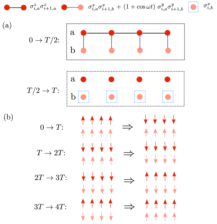
Figure 1: (a) Schematics of our periodically driven spin-1/2 ladder for $N_{0}=4$. During the first half of the period ($0\rightarrow T/2$, solid box), the evolution is governed by externally driven Heisenberg spin exchange interactions that are continuously modulated at frequency $\omega$. In the second half of the period ($T/2\rightarrow T$, dashed box), the interactions are switched off and instead a magnetic field $M$ is applied in the $x$ direction . (b) The 4T-periodic oscillations can be intuitively understood in the solvable limit of $JT=0$ and $hT=MT=\pi$. With all spins initialized pointing up, the system exhibits undergoes spatially uniform 4T-periodic oscillations; ironically, these oscillations become stablized if a nonzero $JT$ is introduced. We remark that an additional phase factors of $i$ or $(-1)$ is omitted in the illustration.

Evidence of robust $4T$-DTC via tMPS.– Here, we employ an efficient method of time evolution with matrix product states (tMPS), where the quantum state is represented as an MPS, and the unitary time evolution operator as an matrix product operator (MPO) [59]. To perform a tMPS study of the system, all the sites are realigned on a linear chain of length $N=2N_{0}$ with next-to-nearest neighbor couplings. We then implement a first-order Suzuki-Trotter algorithm with swap gates [60, 61] to carry out the time-evolution, the mathematical details of which could be found in the supplementary materials [62]. The illustration for the tMPS calculation of the model, numerical details, as well as the transformed Hamiltonian, is also shown in the supplementary materials [62].

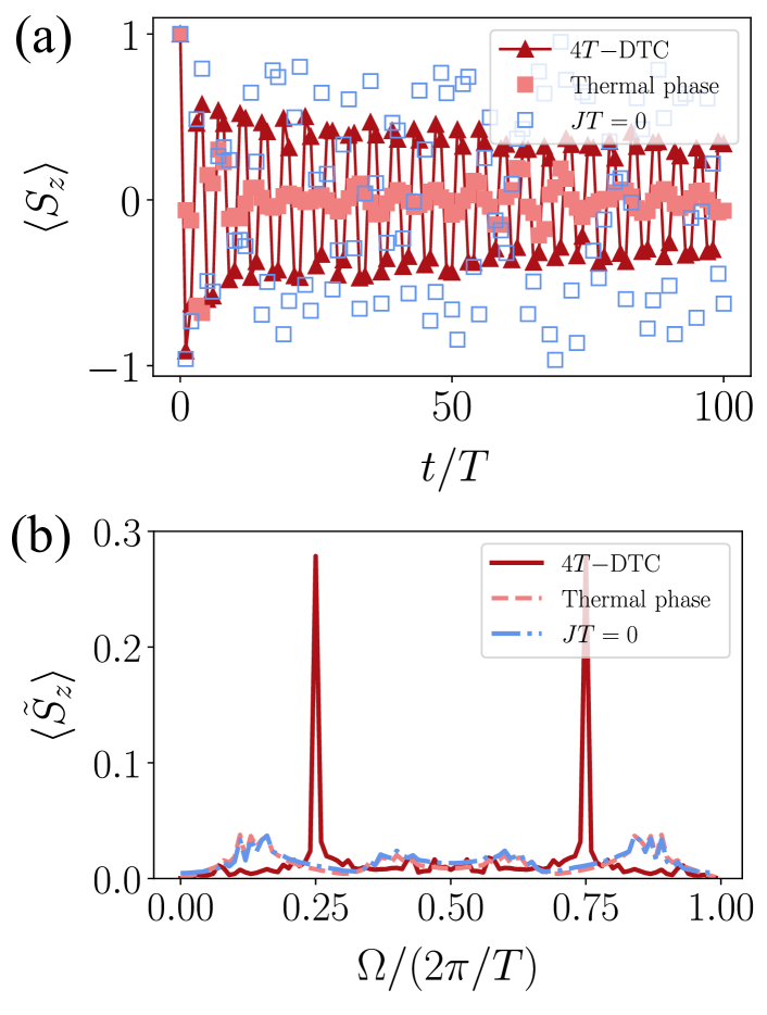
Figure 2: Numerical evidence of robust $4T$-DTC for $N=16$ sites using tMPS. (a) Magnetization $\langle S_{z}\rangle$ as a function of time at $MT=0.98\pi$, which is slightly perturbed away from the ”ideal” solvable limit value $MT=\pi$. For $hT=0.9\pi$, which is also perturbed from $\pi$, nonzero interaction strength $JT=0.16\pi$ (4T-DTC) gives distinctively 4T-periodic oscillations, while $JT=0$ (blue squares) gives random-looking oscillations. The thermal phase at $JT=0.1\pi$, $hT=0.52\pi$ exhibits subdued oscillations. (b) The associated stroboscopic power spectrum $\langle\tilde{S}_{z}\rangle$, which shows distinct frequency peaks at $\Omega=\pm\pi/2T$ only for the 4T-DTC phase.

To capture the signatures of $4T$-DTC in our system, we calculate the stroboscopic averaged magnetization dynamics for spins residing on one of the ladders (which we choose as $a$)

$$\langle S_{z}\rangle\left(t\right)=\frac{1}{N_{0}}\sum_{i=1}^{N_{0}}\langle\sigma_{i,a}^{z}\rangle\left(t\right),$$ (3)

and the associated power spectrum as

$$\langle\tilde{S}_{z}\rangle\left(\Omega\right)=\left|\frac{1}{\mathcal{N}_{\rm tot}}\sum_{k=1}^{\mathcal{N}_{\rm tot}}\langle S_{z}\rangle\left(t\right)\exp{\left[-\frac{k\Omega T}{\mathcal{N}_{\rm tot}}\right]}\right|$$ (4)

where $\mathcal{N}_{\rm tot}$ is the total stroboscopic steps evolved, and $t=kT$ ($k=1,2,\cdots,\mathcal{N}_{tot}$) is the stroboscopic time at step $k$. Our results are summarized in Fig. 2 for two different sets of parameter values that correspond to the $4T$-DTC phase and the thermal phase respectively. Specifically, as the parameters $h$ and $M$ are chosen close to but not equal to the solvable limit values, at a finite value of the inter-site interaction $J$, the period-quadrupling feature of $\langle S_{z}\rangle$ is clearly observed (triangle markers in Fig. 2(a)). This is further demonstrated by a sharp peak at the subharmonic frequency components $\Omega=\pi/2,3\pi/2$ in the power spectrum of Fig. 2(b). That such a $4T$-periodicity is observed over a window of parameter values and not only at a specific set of parameter values suggests that the system indeed supports a $4T$-DTC phase. If a parameter $h$ or $M$ deviates significantly from its corresponding ideal value, or if the inter-site interaction $J$ is absent, $\langle S_{z}\rangle$ quickly decays to zero, and the system is in the thermal phase (empty square and triangle markers in Fig. 2(a)).

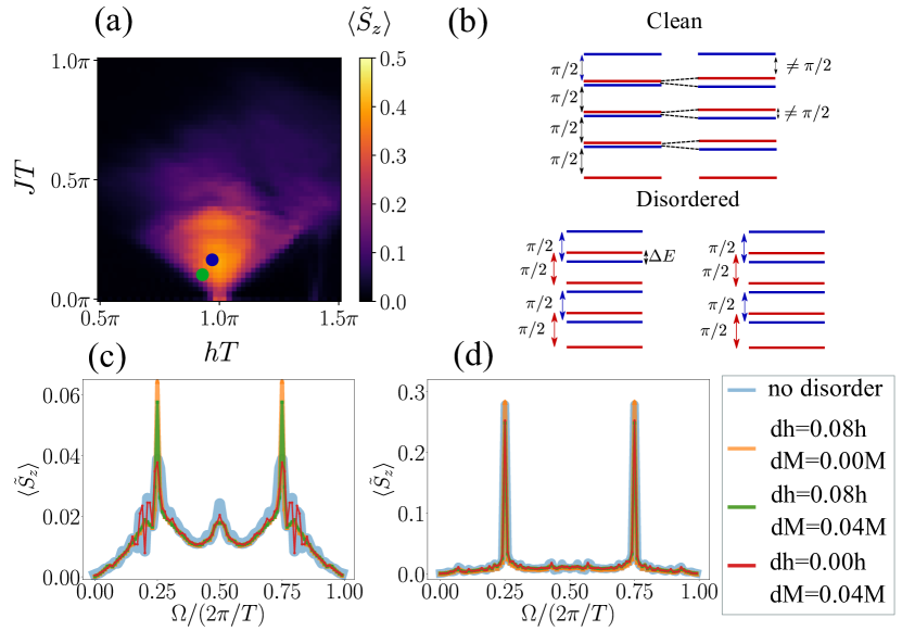
Figure 3: (a) Presence of $4T$-DTC behavior over a wide range of $JT$ and $hT$. The phase diagram representing the value of the subharmonic peak at $\Omega T=\pi/2$ and $MT=0.98\pi$. (b) Illustration of how partial degeneracy in the clean system (overlapping blue and red lines) leads to the breakdown of the $\pi/2$ quasienergy spacing. The left (right)-side quasienergy spacings correspond to the ones before (after) perturbations. (c-d) The full power spectrum associated with the magnetization dynamics up to $t=100T$ under the influence of various disorders at (c) $JT=0.13\pi$, $hT=0.8\pi$, and $MT=0.98\pi$, i.e., green dot in panel a, and (d) $JT=0.16\pi$, $hT=0.9\pi$, and $MT=0.98\pi$, i.e., blue dot in panel a. The enhanced subharmonic peaks due to disorders are clearly observed near the DTC-thermal phase boundaries (panel c). All data points involving disorders are averaged over $220$ realizations.

In Fig. 3(a), we obtain the phase diagram of the system by plotting the subharmonic $\Omega T=\pi/2$ peak ($\langle\tilde{S}_{z}\rangle\left(\Omega\right)$ at $\Omega=\pi/2T$) in the power spectrum against the two system parameters $h$ and $J$ for the system size of $N=16$. There, a finite (zero) $\langle\tilde{S}_{z}\rangle\left(\Omega\right)$ at $\Omega=\pi/2T$ is associated with the the $4T$-DTC (thermal) phase. It is observed that the $4T$-DTC phase spans over a considerable window of $h$ values – symmetrically about $hT=\pi$–at moderate values of $J$. At $J=0$, the period-quadrupling feature is observed only at $hT=\pi$, further confirming the role of the inter-site interaction in stabilizing the DTC phase. On the other hand, at very large values of $J$, the $4T$-DTC behavior is absent altogether, which could be attributed to the presence of quantum chaos [63].

In Fig. 3(c) and (d), we investigate the effect of spatial disorder on our $4T$-DTC system, with the surprising revelation that disorder can actually enhance the signature of a $4T$-DTC phase near its border with a thermal phase. (d) is chosen deep in the DTC regime, whereas (c) is taken near the border between DTC and thermal phase. Here, each of the disordered parameters $h$, $J$, and $M$ for each spin in the system is drawn randomly from a uniform distribution of $[P-dP+P+dP]$, where $P=h,J,M$ and $dP=dh,dJ,dM$.

Figs. 3(c) and (d) present the striking observation that the presence of disorder actually enhances the signature of a $4T$-DTC phase near its border with a thermal phase. To understand this result, we should first recall that in a genuine $4T$-DTC, a macroscopic number of quasienergies (the eigenphases of the one-period evolution operator) form quadruplets with $\pi/2$ spacing among them, i.e., they can be written as $\varepsilon+n\pi/2$ for some $\varepsilon$ and $n=0,1,2,3$ [20, 58]. Ideally, such quadruplets of quasienergies should be either non-degenerate or fully degenerate ($\varepsilon+n\pi/2$ for all $n$). In the case of partial degeneracy, i.e., $\varepsilon+n\pi/2$ are only degenerate for some $n$, certain perturbations may nonuniformly shift those degenerate quasienergies [see the upper part of Fig. 3(b)], which then breaks their $\pi/2$ quasienergy spacing and consequently leads to a less robust period-quadrupling signal. In the clean system, such partial degeneracy tends to occur very often; perturbing the system parameters near the DTC-thermal phase transitions then causes the many quadruplets of $\pi/2$-separated quasienergies above to break down due to the aforementioned mechanism. In the presence of spatial disorder, the system parameters for each spin or pair of spins take on slightly different values. As a result, the probability for a system’s quasienergy to be degenerate is significantly reduced, thereby resulting in more robust $\pi/2$-separated quadruplets of quasienergies [see the lower part of Fig. 3(b)]. In the Supplemental Material [62], we further demonstrate the above argument by explicitly evaluating the quasienergy levels with and without disorder.

Away from the phase transition boundaries, the presence of disorders does not seem to yield a signal improvement. In some cases, disorders instead slightly reduce the subharmonic peak. Indeed, away from the phase transition boundaries (close to the solvable limit), the detrimental partial degeneracy among different quadruplets of $\pi/2$-separated quasienergies is already rare to begin with. In this case, disorders instead serve as perturbations in the system parameters with respect to the solvable limit values. Nevertheless, as demonstrated in Fig. 3(c) and (d), our DTC is remarkably robust against moderate disorders ($\sim 8\%$).

Our numerical findings indicate that these spatial disorders enhance the distinguishing features of the $4T$-DTC near its borders with the thermal phase. When deep within the DTC phase, spatial disorders have a tendency to marginally reduce the strength of its distinguishing signatures, although they still remain clearly discernible, which demonstrates the robustness of our $4T$-DTC.

Realization of robust $4T$-DTC on a quantum processor.– In the numerical simulations of our model using tMPS, we have uncovered that the signature of $4T$-DTC is extremely robust, even in the presence of spatial disorders. This suggests that our model is ideal for physically realizing on the quantum computer, which inevitably exhibits various types of device noise. Particularly, given that other simulations of DTC realized in quantum computers exhibit poor results due to the effect of noise [64, 65], our $4T$-DTC model not only possesses Heisenberg spin exchange interactions beyond Ising-type couplings [51], but also holds the promise for much more robust signatures.

Here, we proceed to realize our system, and capture its DTC signatures on the IBMQ quantum processor. Naive implementation of the time dynamics of our model in a quantum circuit follows from a similar trotterization procedure as in our tMPS simulations, and more details are shown in the Supplementary Materials [62]. For any quantum circuit implementation, the coupling between qubits needs to be implemented via basic quantum gates such as the controlled NOT (CNOT) and the single-qubit rotation gates; one significant advantage of a quantum circuit implementation over other quantum platforms i.e. ultracold atoms is that a time-dependent model such as a DTC model can implemented without any additional difficulty, just by concatenating different Trotter steps at different stages. Instead of transpiling local couplings within each Trotter step, we adopt a more efficient approach by leveraging the variational circuit optimization technique, and the details of this approach are presented in the Suupelemntary Materials [62]. This strategy of directly implementing the whole circuit requires fewer $CX$ gates and compresses the circuit depth, thereby suppressing the effect of gate error. For other simulations using the Trotterization approach [64, 65], the signature of the DTC gets poorer under evolving dynamics, as the circuit depth itself grows linearly. In our unique scheme of trained circuits with a fixed circuit depth, as demonstrated below, we successfully achieve robust results for our proposed $4T$-DTC model, and in particular, it exhibits remarkably strong resilience to device noise even during many Floquet cycles.

In Fig. 4, we present our measured the stroboscopic magnetization $\langle S_{z}\rangle$ (solid circles) on the IBM quantum computer over time dynamics and compared these with the numerical results (unfilled circles, squares, and triangles) obtained by the tMPS method. Remarkably, thanks to our variational method, we realize the quantum simulation over long periods of time ($20$ Floquet steps). Within such long-time dynamics, our numerical and quantum results demonstrate an excellent agreement, indicating that our IBM Q simulation gives a perfect characterization of our $4$-DTC model. Here, we execute our IBM Q simulation on an 8-qubit case which enables the realization of highly-compressed trained circuits for overcoming device noise . This is already a sufficiently long chain for demonstrating 4T-DTC, given that finite-size effects are insignificant as shown in Fig. 4, as evidenced by the fact that by our tMPS results at different sizes $N=8,16$, and $32$ all show qualitatively similar profiles with the IBM Q results.

Figure 4: Physical signature of $4T$-DTC behavior on the IBM quantum processor and its comparison with tMPS results at several system sizes (green). The parameters used are: $JT=0.5\pi$, $MT=0.98\pi$, $hT=0.9\pi$. For the details of the device ibmq_cairo and its error information, see Fig. S5 in the supplementary materials [62].

Conclusion and outlook.– We proposed an intuitive and realistic new spin-1/2 model that supports a nontrivial type of DTC, characterized by a robust period-quadrupling observable rather than the more common period-doubling type. Remarkably, we were able to explicitly capture the signatures of such $4T$-DTC both numerically and via a NISQ-era IBM quantum processor, even at relatively small number of qubits and in the presence of considerable hardware noise. In particular, excellent agreement was obtained between the two approaches. More surprisingly, we found that spatial disorders could actually improve the signatures of $4T$-DTC in some cases, thus shedding more light on the role of disorders in the formation of DTCs.

The experimental realization of our $4T$-DTC system at larger system sizes is expected to be a significant future research direction, both in the area of quantum computing and in condensed matter platforms such as ultracold atoms [67, 68, 69, 70, 71, 72, 73, 74, 75, 38, 76]. On the one hand, that our $4T$-DTC phase exists within a spin-1/2 system makes it a realistic and appropriate phenomenon for benchmarking the performance of various existing noisy intermediate-scale quantum (NISQ) devices. On the other hand, the ability to achieve a large size $4T$-DTC may also open up opportunities to harness its technological application beyond observing its subharmonic signatures, e.g., as a quantum memory or a passive quantum error correcting device. Finally, a realistic generalization of our spin-1/2 system construction that supports DTCs beyond period-quadrupling makes for a good avenue for future theoretical and experimental studies that can uncover rich phenomenology lying in the intersection of Floquet, many-body or even non-Hermitian physics.

Acknowledgements.– We are grateful to Jiangbin Gong for fruitful discussions. T. C. thanks E. Miles Stoudenmire for fruitful discussion via ITensor discourse group [77]. T. C. and R. S. thank Truman Ng and Russell Yang for discussions on the quantum simulation implementation on IBM Quantum services. C. H. L. and T. C. acknowledges support by Singapore’s NRF Quantum engineering grant NRF2021-QEP2-02-P09 and Singapore’s MOE Tier-II grant Proposal ID: T2EP50222-0008. T. C. and B. Y. acknowledges the support from Singapore National Research Foundation (NRF) under NRF fellowship award NRF-NRFF12-2020-0005. R. W. B acknowledges the support provided by the Deanship of Research Oversight and Coordination (DROC) at King Fahd University of Petroleum & Minerals (KFUPM) through project No. EC221010. We acknowledge the use of IBM Quantum services for this work. The views expressed are those of the authors, and do not reflect the official policy or position of IBM or the IBM Quantum team. The MPS calculation in this work is performed using ITensor library [78]. The computational work for this article was partially performed on resources of the National Supercomputing Centre, Singapore (https://www.nscc.sg/), and on the National University of Singapore (NUS)’s high-performance computing facilities.

Supplementary Materials for “Signatures of a Robust Large-Period Discrete Time Crystal”

S1 Robustness of $\pi/2$ quasienergy spacing in the presence of disorder

In the main text, we discussed that the positive effect of disorder observed near the DTC-thermal phase boundaries is attributed to the preservation of the $\pi/2$ quasienergy spacing among the quadruplets of quasienergies. In this section, we verify this argument by explicitly computing the full quasienergy spectrum of our system (via exact diagonalization) at the same system paramaters as those of Fig. 3 in the main text. In particular, a quasienergy $\varepsilon$ is obtained from the eigenvalue $e^{-\mathrm{i}\varepsilon}$ of the (unitary) one-period time evolution operator.

Our results are summarized in Fig. S1, where we have shown some representative quasienergy levels of the system with and without disorders. In particular, for each data point, the blue circle marks the $j$th quasienergy solution, i.e., $\varepsilon_{j}$, whereas the corresponding green square (red triangle) marks some other quasienergy solution, e.g., $\varepsilon_{\ell}$ whose value is the closest to $\varepsilon_{j}+\pi/2$ ($\varepsilon_{j}-\pi/2$). Therefore, note that for the many-body quasienergy levels to contain a macroscopic number of $\pi/2$-quasienergy separated quadruplets, the majority of the red triangles, green squares, and blue circles in Fig. S1 must coincide with one another. As is clear from the figure, this is the case when disorder is present (panel b). In the absence of disorder (panel a), a significant number of quasienergy solutions do not coincide with any other quasienergy solution when shifted by $\pm\pi/2$. This in turn explains the stronger DTC signal observed in Fig. 3(c) of the main text when disorder is present.

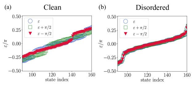
Figure S1: Representative quasienergy solutions $\varepsilon$ (blue circles) and the quasienergies that are closest to them upon shifting by $\pm\pi/2$ (see the discussion of Sec. S1 for the exact definitions) in (a) the absence of disorder and (b) the presence of spatial disorder with $dh=0.08h,dM=0.08M$. The system size is taken at $N=8$ in both panels and all other parameters used are the same as in Fig. 3(c) of the main text, i.e., $JT=0.13\pi,hT=0.8\pi,MT=0.98\pi$. Notably, the degeneracy modulo $\pi/2$ is stronger when disorder is present, thereby explaining the more robust 4T-periodicity when disorder is present.

S2 Details of Suzuki-Trotter decomposition and time evolution on IBM Q

We start by discussing how to simulate the dynamics of our model in Eq. (S2) on a quantum circuit digitally. First, within each period $T$, the time evolution operator $\hat{U}$ operates as

$$\hat{U}|\psi_{0}\rangle=\hat{U}_{T/2\rightarrow T}\hat{U}_{0\rightarrow T/2}|\psi_{0}\rangle$$ (S1)

where $|\psi_{0}\rangle$ is the initial state, $\hat{U}_{0\rightarrow T/2}$ is the evolution operator for the first-half period, and $\hat{U}_{T/2\rightarrow T}$ is the evolution operator for the second-half period. We remark that for the tMPS simulation, the total system needs to be aligned as a linear chain with some of the terms having next-nearest neighbor couplings [see Fig. S2], and the Hamiltonian thus becomes

$$\hat{\mathcal{H}}\left(t\right)=\begin{cases}-h/2\sum_{i=1}^{N_{0}}\left(H_{i}^{xx}-H_{i}^{yy}\right)-JH_{i}^{zz}&\quad 0<t<\frac{T}{2},\\ M\sum_{i=1}^{N_{0}}\sigma_{2i}^{x}&\quad\frac{T}{2}<t<T.\end{cases}$$ (S2)

where

$$H_{i}^{xx}=\sigma_{2i-1}^{x}\sigma_{2i}^{x}$$ (S3)

$$H_{i}^{yy}=\left(1+\cos{\omega t}\right)\sigma_{2i-1}^{y}\sigma_{2i}^{y}$$

$$H_{i}^{zz}=\sum_{i=1}^{N_{0}-1}\sigma_{2i-1}^{z}\sigma_{2i+1}^{z}$$

For each half period, we could therefore consider applying the first-order Suzuki-Trotter decomposition, and obtain the first half of $U$ as follows

$$\hat{U}_{0\rightarrow T/2}\approx\prod^{T/\delta t}_{n=0}\left[\prod_{i=0}^{N/4-1}e^{+i\delta tJ\sigma_{2i+2}^{z}\otimes I_{2i+3}\otimes\sigma_{2i+4}^{z}}\prod_{i=0}^{N/4}e^{+i\delta tJ\sigma_{2i}^{z}\otimes I_{2i+1}\otimes\sigma_{2i+2}^{z}}\right]$$ (S4)

$$\left[\prod_{i=0}^{N/2}e^{+i\delta th/2\left(\sigma_{2i}^{x}\otimes\sigma_{2i+1}^{x}-\left(1+\cos{\omega n\delta t}\right)\sigma_{2i}^{y}\otimes\sigma_{2i+1}^{y}\right)}\right],$$

where $\delta t$ is the discretized time step, which is set to be $0.01/T$ ($T=1$) in our numerics. Note that for the next-nearest neighbor coupling terms in the above expression, for the simulation on IBM Q, it only requires a pair of swap gates between the ancilla qubit ($i=4$) and the physical qubit ($i=6$) with system size $N=8$ [see Fig. S5(d)], while for the simulation with tMPS, since it is aligned to a linear spin chain, for a system size of $N$ (assume $N$ is always even in this case), it requires $(N/2-1)$ pairs of the swap gates [60, 79]. Finally, the second-half time evolution operator $\hat{U}_{T/2\rightarrow T}$ can be simply realized by the following $R_{x}$ rotations

$$\hat{U}_{T/2\rightarrow T}=\prod^{N/2}_{i=0}e^{-i\frac{MT}{2}\sigma_{2i+1}^{x}}.$$ (S5)

Throughout this manuscript, we take the evolution time step for our tMPS algorithm as $0.01\hbar$, and the convergences of the tMPS calculations are confirmed by checking the truncation errors after repeating the runs for different values of the maximum bond dimension. We find that keeping a a maximum auxiliary bond dimension of $100$ for $N=24$ and $N=32$, $60$ for $N=16$ and $N=8$ for all tMPS calculations allows us to produce precise simulations, with errors on the observables of, at most, $10^{-8}$.

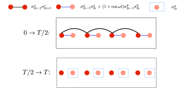
Figure S2: Illustration of schematical tMPS with Suzuki-Trotter decomposition. The total system from Fig. 1 is now mapped into a single chain with alternative nearest neighbor and next-nearest neighbor couplings.

S3 $4T$-DTC results for a larger system size of $N=32$

In this section, we supplement our tMPMs results presented in Figs. 2 and 3 of the main text with those calculated at a larger system size of $N=32$. Our results, which are summarized in Figs. S3 and S4 of the Supplementary Materials, display qualitatively the same features as those obtained in the main text. That is, the period-quadrupling signature of the $4T$-DTC is not only robust against a variety of spatial disorders (see Fig. S3), but it may get amplified in some cases (see Fig. S4).

Figure S3: Numerical evidence of robust $4T$-DTC for $N=32$ sites using tMPS. (a)-(c) Stroboscopic magnetization $\langle S_{z}\rangle$ as a function of time. (d)-(f) The power spectrum $\langle\tilde{S}_{z}\rangle$. In panel a and d, the darker red data is taken at $J=0.16\pi$, $M=0.98\pi$, and $h=0.9\pi$ (which corresponds to the $4T$-DTC phase regime in Fig. 3(a) of the main text), and the lighter red data is taken at $J=0.1\pi$, $M=0.98\pi$, and $h=0.52\pi$ (which corresponds to the thermal phase regime in Fig. 3(a) of the main text). In panel b and e, the data points correspond to no disorder (red), $dh=0.12h$ (green), and $dJ=0.12J$ (blue). In panel c and f, the data points are taken at no disorder (red) and $dM=0.12M$ (green). In all panels, the system size is $N=32$, $T$ is set to be $1$, and all disorder results are averaged over $220$ disorder realizations, each of which is equally drawn from the corresponding interval. Numerically, it is found that for larger system size such as $N=32$, our $4T$-DTC model is still robust against a variety of spatial disorders.

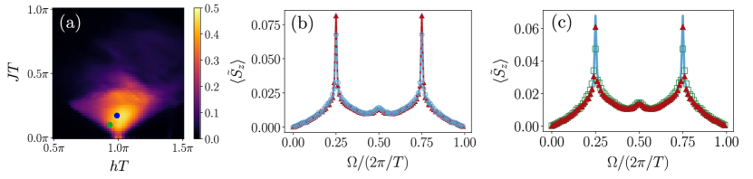
Figure S4: (a) The phase diagram representing the value of the subharmonic peak at $\Omega=\pi/2$ and $MT=0.98\pi$, numerically computed for a large $N=32$ system size. The $4T$-DTC phase is nearly symmetric, and spans over a considerable window of $h$ values, which are symmetrically about $hT=\pi$ and at moderate values of $J$. (b,c) The numerically calculated power spectrum $\langle\tilde{S}_{z}\rangle$ over $100$ periods at $JT=0.13\pi$, $hT=0.8\pi$, $MT=0.98\pi$ with (b) no disorder (blue); $dh=0.08h$ (red). (c) without disorder (blue); only $dM=0.04M$ (green); both $dM=0.04M$ and $dh=0.08h$ (red). The result without disorder corresponds to parameters at the boundary between the thermal phase and the DTC phase, i.e. the green dot in panel (a), while to blue dot corresponds to the results from Fig. S3(b), (c), (e) and (f). The system size is taken at $N=32$ in all panels and all data points involving disorders in panels b and c are averaged over $220$ disorder realizations. From the power spectrum peak in panel (b) and (c) at $\Omega T=\pi/2$, it is shown that the period-quadrupling signature of the $4T$-DTC is also enhanced for spatial disorder $dh$.

Figure S5: The geometry and error information of IBM Q device ibmq_cairo and details of the variational circuit recompilation algorithm. (a) The snapshot taken from IBM Q (on June 20, 2023) for CNOT ($CX$) gate error and readout error. Here, the readout error is represented by the coloring on the qubit sites, whereas the $CX$ gate error is represented by the coloring on the links connecting nearest-neighboring qubits. (b) An example of qubits choices (grey circles) of which the geometry is consistent with the configuration shown in panel (d). (c) The quantum circuit for the Trotterized time evolution is transformed into a parameterized quantum circuit suitable for execution on an IBM quantum processor via optimization on a classical computer. (d) (upper panel) The configuration of the quantum circuit with the additional ancilla qubit. (lower panel) The next-to-nearest neighbor $CX$ gate can be exactly decomposed to nearest-neighbor two-body gates.

S4 Variational algorithm for the time evolution on IBM Q

In this section, we describe our implementation of the variational algorithm to perform the time evolution of our model in the main text on digital quantum computers, specifically the IBM Q quantum processors.

S4.1 Details the IBM quantum processor and its error rates

First, we show the details of error and the choices of qubits on the $27$-qubit Falcon IBM quantum processor ibmq_cairo, which we have utilized throughout this work. The error profile of the device is shown Fig. S5(a), encompassing both $CX$ (CNOT) gate errors as well as readout assignment errors, as depicted by the colors in the circles (readout assignment errors) and the bonds (gate errors). In Fig. S5(b), we show the choice of $N=8+1$ qubits (grey circles) which we used to represent our system, indexed $0$ to $8$, which is consistent with the circuit configuration in the main text.

S4.2 Variational circuit recompilation of the time evolution operators

In the current NISQ-era of quantum computing, variational quantum algorithms (VQAs) have proven to be effective due to their reduced gate counts, as discussed in references [80, 81]. VQAs involve a two-step process where parameterized circuits are first generated on a classical computer through an optimization algorithm. Then, these circuits with optimized parameters are executed on the quantum computer. Therefore, we explore a variational approach referred to as ’circuit recompilation’ (detailed in references [82, 83, 84, 85, 86]), which has shown promise in providing accurate approximations to the original unitary transformations while requiring much shorter circuit depths and fewer $CX$ and single-qubit gates compared to the default isometry decomposition. This approach results in significantly reduced overall gate errors when using current NISQ-era quantum processors [43].

Here, we provide the details of our variational quantum circuit recompilation for the time evolution operators used in the main text. The scheme of our variational algorithm to obtain the parametrized quantum circuit is depicted in Fig. S5(c) and (d). The original time evolution circuit $\hat{\mathcal{U}}$ with Suzuki-Trotter gates is transformed into a Trotterized ansatz circuit $\hat{\mathcal{V}}$ via variational optimization [Fig. S5(c)]. For each stroboscopic time step $t=kT$ ($k=1,2,\cdots,\mathcal{N}_{\rm tot}$), it is transformed into an ansatz $\hat{\mathcal{V}}(t=kT)$, which consists of an initial layer of $U_{3}$ gates followed by concatenated odd layers (green) and even layers (purple) [82, 87, 83, 88, 85][Fig. S5(c)], which has a Trotterized time evolution pattern. Here, we set all number of total layers to be equal to be three, i.e. it has in total three combined layers of odd and even layers. Also, we follow the definitions of $3D$ rotation $U_{3}$ gates from Qiskit [89]:

$$\begin{aligned} \hfil\displaystyle\begin{split}U_{3}(\theta,\phi,\lambda)=\begin{pmatrix}\cos\left(\frac{\theta}{2}\right)&-e^{i\lambda}\sin\left(\frac{\theta}{2}\right)\\ e^{i\phi}\sin\left(\frac{\theta}{2}\right)&e^{i(\phi+\lambda)}\cos\left(\frac{\theta}{2}\right)\end{pmatrix}\end{split}\end{aligned}$$ (S6)

where $\theta,\phi,\lambda\in[0,2\pi]$.

The circuit variational optimization is done by minimizing the cost function

$$F(\hat{\mathcal{U}},\hat{\mathcal{V}})=1-\langle\psi_{0}|\hat{\mathcal{V}}^{\dagger}\hat{\mathcal{U}}|\psi_{0}\rangle$$ (S7)

where we have deliberately chosen the initial $|\psi_{0}\rangle$ with all sites in $|\uparrow\rangle$. The process of the circuit variational optimization involves optimizing a $3D$ rotation gate labeled as $U_{3}(\theta,\phi,\lambda)$. This gate is characterized by three rotational parameters which are variable: $\theta$, $\phi$ and $\lambda$. The optimization is carried out using the Limited Memory Broyden-Fletcher-Goldfarb-Shanno algorithm with box constraints (L-BFGSB), as outlined in Refs. [90, 91, 85]. To prevent getting stuck in local minimums during the optimization, we employ a basin-hopping technique [92, 93, 94, 95]. Here, small perturbations are introduced in each optimization iteration, which are then followed by local minimization steps.

In addition, due to the IBM quantum device configuration geometry, an additional ancilla qubit [green circle, Fig. S5(d)] is required such that the Heisenberg spin $zz$ interactions can be realized with one $CX$ gate plus two swap gates on IBM Q [Fig. S5(d)], and therefore the model configuration with $N=8$ (system) $+1$ (ancilla qubit) is consistent with the device [Fig. S5(b)]. To simulate a larger system size, encompassing more than 10 qubits, our model described by Eq. (1) in the main text is inherently scalable. It can be mapped to a two coupled one-dimensional chains, where each unit cell consists of two sites labeled as $a$ and $b$. In this case, the interactions between $a$ sites become next-nearest-neighbor-couplings. Such a setup can be easily achieved via the technique of circuit recompilation [85].

S4.3 Measurement, observables and error mitigation on IBM Q

The magnetization in the $z$ direction for each spin residing on ladder a from our model is obtained via the measurement procedure on IBM quantum processor, which is performed after the time evolution in the Trotterized ansatz circuit $\hat{\mathcal{V}}$. On IBM Q, the measured outcomes are all represented in binary bit strings, i.e. $0$ for spin-up ($|\uparrow\rangle$), and $1$ for spin-down ($|\downarrow\rangle$). For each site $i$, the magnetization in the $z$ direction for each spin residing on ladder a $\langle\sigma_{i,a}^{z}\rangle$ is computed as

$$\langle\sigma_{i,a}^{z}\rangle=\langle\sigma_{i,a}^{\uparrow}\rangle-\langle\sigma_{i,a}^{\downarrow}\rangle$$ (S8)

where $\sigma^{\uparrow}=\begin{pmatrix}1&0\\ 0&0\end{pmatrix}$, and $\sigma^{\downarrow}=\begin{pmatrix}0&0\\ 0&1\end{pmatrix}$.

Then, the stroboscopic averaged magnetization dynamics from Eq. (3) as well as the associated power spectrum from Eq. (4) in the main text can all be easily obtained from the above results.

One major issue we address in our IBM Q experiment is the readout assignment error [see also Fig. S5(a)]. This issue involves the possibility of mistakenly measuring an $|\uparrow\rangle$ state as $|\downarrow\rangle$ and vice versa. Recent advancements have made significant progress in reducing measurement errors, as documented in several studies [96, 97, 98, 99, 100, 101, 102]. In the context of the Qiskit environment [89], one approach involves running calibration circuits with various initial conditions and then using the resulting data to estimate accurate measurement counts based on a calibration matrix [103, 104]. However, in our paper, we employ a novel readout error mitigation method [105] that requires only a small number of circuits, eliminating the need to construct a full calibration matrix, and is ready to use with their Python package integrated with the Qiskit environment [89].

To align with the job submission framework of the IBM Q platform and optimize the calibration process, we combine the circuits responsible for performing the time evolution (referred to as ”physical circuits”) with the calibration circuits as mentioned above into a single job submitted to the IBM Q cloud platform. This ensures that the physical circuits and calibration circuits are executed nearly simultaneously, enhancing the accuracy of the calibration process. Additionally, to maintain a consistent quantum register layout for both physical and calibration circuits, we first select and transpile the physical circuit for the specific real device using device error data calibrated by IBM Q for high-fidelity quantum nondemolition (QND) measurements [85]. We then apply this layout to the calibration circuit, ensuring that the same qubits are used for both categories of circuits. Finally, we submit both types of circuits together to the IBM Q real device for execution.

References

- Hardy and Binek [2014] R. J. Hardy and C. Binek, Thermodynamics and statistical mechanics: an integrated approach (John Wiley & Sons, 2014).
- Anderson [1972] P. W. Anderson, More is different, Science 177, 393 (1972).
- Deutsch [1991] J. M. Deutsch, Quantum statistical mechanics in a closed system, Phys. Rev. A 43, 2046 (1991).
- Srednicki [1994] M. Srednicki, Chaos and quantum thermalization, Phys. Rev. E 50, 888 (1994).
- Murthy et al. [2023] C. Murthy, A. Babakhani, F. Iniguez, M. Srednicki, and N. Yunger Halpern, Non-abelian eigenstate thermalization hypothesis, Phys. Rev. Lett. 130, 140402 (2023).
- Nandkishore and Huse [2015] R. Nandkishore and D. A. Huse, Many-body localization and thermalization in quantum statistical mechanics, Annu. Rev. Condens. Matter Phys. 6, 15 (2015).
- Abanin et al. [2019] D. A. Abanin, E. Altman, I. Bloch, and M. Serbyn, Colloquium: Many-body localization, thermalization, and entanglement, Rev. Mod. Phys. 91, 021001 (2019).
- Serbyn et al. [2021] M. Serbyn, D. A. Abanin, and Z. Papić, Quantum many-body scars and weak breaking of ergodicity, Nature Physics 17, 675 (2021).
- Chandran et al. [2023] A. Chandran, T. Iadecola, V. Khemani, and R. Moessner, Quantum many-body scars: A quasiparticle perspective, Annual Review of Condensed Matter Physics 14, 443 (2023).
- D’Alessio et al. [2016] L. D’Alessio, Y. Kafri, A. Polkovnikov, and M. Rigol, From quantum chaos and eigenstate thermalization to statistical mechanics and thermodynamics, Advances in Physics 65, 239 (2016).
- Wilczek [2012] F. Wilczek, Quantum time crystals, Phys. Rev. Lett. 109, 160401 (2012).
- Bruno [2013] P. Bruno, Impossibility of spontaneously rotating time crystals: A no-go theorem, Phys. Rev. Lett. 111, 070402 (2013).
- Watanabe and Oshikawa [2015] H. Watanabe and M. Oshikawa, Absence of quantum time crystals, Phys. Rev. Lett. 114, 251603 (2015).
- Sacha and Zakrzewski [2017] K. Sacha and J. Zakrzewski, Time crystals: a review, Reports on Progress in Physics 81, 016401 (2017).
- Khemani et al. [2019] V. Khemani, R. Moessner, and S. Sondhi, A brief history of time crystals, arXiv:1910.10745 (2019).
- Yao et al. [2017] N. Y. Yao, A. C. Potter, I.-D. Potirniche, and A. Vishwanath, Discrete time crystals: Rigidity, criticality, and realizations, Phys. Rev. Lett. 118, 030401 (2017).
- Else et al. [2016] D. V. Else, B. Bauer, and C. Nayak, Floquet time crystals, Phys. Rev. Lett. 117, 090402 (2016).
- Else et al. [2020] D. V. Else, C. Monroe, C. Nayak, and N. Y. Yao, Discrete time crystals, Annual Review of Condensed Matter Physics 11, 467 (2020).
- Zaletel et al. [2023] M. P. Zaletel, M. Lukin, C. Monroe, C. Nayak, F. Wilczek, and N. Y. Yao, Colloquium: Quantum and classical discrete time crystals, Rev. Mod. Phys. 95, 031001 (2023).
- Bomantara [2021] R. W. Bomantara, Quantum repetition codes as building blocks of large-period discrete time crystals, Phys. Rev. B 104, L180304 (2021).
- Guo et al. [2013] L. Guo, M. Marthaler, and G. Schön, Phase space crystals: A new way to create a quasienergy band structure, Phys. Rev. Lett. 111, 205303 (2013).
- Sacha [2015a] K. Sacha, Anderson localization and mott insulator phase in the time domain, Scientific reports 5, 10787 (2015a).
- Delande et al. [2017] D. Delande, L. Morales-Molina, and K. Sacha, Three-dimensional localized-delocalized anderson transition in the time domain, Phys. Rev. Lett. 119, 230404 (2017).
- Giergiel and Sacha [2017] K. Giergiel and K. Sacha, Anderson localization of a rydberg electron along a classical orbit, Phys. Rev. A 95, 063402 (2017).
- Mierzejewski et al. [2017] M. Mierzejewski, K. Giergiel, and K. Sacha, Many-body localization caused by temporal disorder, Phys. Rev. B 96, 140201 (2017).
- Giergiel et al. [2018] K. Giergiel, A. Miroszewski, and K. Sacha, Time crystal platform: From quasicrystal structures in time to systems with exotic interactions, Phys. Rev. Lett. 120, 140401 (2018).
- Guo and Liang [2020] L. Guo and P. Liang, Condensed matter physics in time crystals, New Journal of Physics 22, 075003 (2020).
- Sacha [2015b] K. Sacha, Modeling spontaneous breaking of time-translation symmetry, Phys. Rev. A 91, 033617 (2015b).
- Surace et al. [2019] F. M. Surace, A. Russomanno, M. Dalmonte, A. Silva, R. Fazio, and F. Iemini, Floquet time crystals in clock models, Phys. Rev. B 99, 104303 (2019).
- Nurwantoro et al. [2019] P. Nurwantoro, R. W. Bomantara, and J. Gong, Discrete time crystals in many-body quantum chaos, Phys. Rev. B 100, 214311 (2019).
- Giergiel et al. [2020] K. Giergiel, T. Tran, A. Zaheer, A. Singh, A. Sidorov, K. Sacha, and P. Hannaford, Creating big time crystals with ultracold atoms, New Journal of Physics 22, 085004 (2020).
- Pizzi et al. [2021] A. Pizzi, J. Knolle, and A. Nunnenkamp, Higher-order and fractional discrete time crystals in clean long-range interacting systems, Nature communications 12, 2341 (2021).
- Zhang et al. [2017] J. Zhang, P. W. Hess, A. Kyprianidis, P. Becker, A. Lee, J. Smith, G. Pagano, I.-D. Potirniche, A. C. Potter, A. Vishwanath, et al., Observation of a discrete time crystal, Nature 543, 217 (2017).
- Rovny et al. [2018a] J. Rovny, R. L. Blum, and S. E. Barrett, Observation of discrete-time-crystal signatures in an ordered dipolar many-body system, Phys. Rev. Lett. 120, 180603 (2018a).
- Rovny et al. [2018b] J. Rovny, R. L. Blum, and S. E. Barrett, nmr study of discrete time-crystalline signatures in an ordered crystal of ammonium dihydrogen phosphate, Phys. Rev. B 97, 184301 (2018b).
- Pal et al. [2018] S. Pal, N. Nishad, T. S. Mahesh, and G. J. Sreejith, Temporal order in periodically driven spins in star-shaped clusters, Phys. Rev. Lett. 120, 180602 (2018).
- Autti et al. [2021] S. Autti, P. J. Heikkinen, J. T. Mäkinen, G. E. Volovik, V. V. Zavjalov, and V. B. Eltsov, Ac josephson effect between two superfluid time crystals, Nature Materials 20, 171 (2021).
- Kyprianidis et al. [2021] A. Kyprianidis, F. Machado, W. Morong, P. Becker, K. S. Collins, D. V. Else, L. Feng, P. W. Hess, C. Nayak, G. Pagano, et al., Observation of a prethermal discrete time crystal, Science 372, 1192 (2021).
- Choi et al. [2017] S. Choi, J. Choi, R. Landig, G. Kucsko, H. Zhou, J. Isoya, F. Jelezko, S. Onoda, H. Sumiya, V. Khemani, et al., Observation of discrete time-crystalline order in a disordered dipolar many-body system, Nature 543, 221 (2017).
- Cheng et al. [2022] Z. Cheng, R. W. Bomantara, H. Xue, W. Zhu, J. Gong, and B. Zhang, Observation of modes in an acoustic floquet system, Phys. Rev. Lett. 129, 254301 (2022).
- Vidal [2004] G. Vidal, Efficient simulation of one-dimensional quantum many-body systems, Phys. Rev. Lett. 93, 040502 (2004).
- Paeckel et al. [2019] S. Paeckel, T. Köhler, A. Swoboda, S. R. Manmana, U. Schollwöck, and C. Hubig, Time-evolution methods for matrix-product states, Annals of Physics 411, 167998 (2019).
- Preskill [2018] J. Preskill, Quantum Computing in the NISQ era and beyond, Quantum 2, 79 (2018).
- Johnstun and Van Huele [2021] S. Johnstun and J.-F. Van Huele, Understanding and compensating for noise on ibm quantum computers, American Journal of Physics 89, 935 (2021).
- Lau et al. [2022] J. W. Z. Lau, K. H. Lim, H. Shrotriya, and L. C. Kwek, Nisq computing: where are we and where do we go?, AAPPS Bulletin 32, 27 (2022).
- Smith et al. [2019] A. Smith, M. Kim, F. Pollmann, and J. Knolle, Simulating quantum many-body dynamics on a current digital quantum computer, npj Quantum Information 5, 106 (2019).
- Rahmani et al. [2020] A. Rahmani, K. J. Sung, H. Putterman, P. Roushan, P. Ghaemi, and Z. Jiang, Creating and manipulating a laughlin-type fractional quantum hall state on a quantum computer with linear depth circuits, PRX Quantum 1, 020309 (2020).
- Google AI Quantum and Collaborators et al. [2020] Google AI Quantum and Collaborators, F. Arute, K. Arya, R. Babbush, D. Bacon, J. C. Bardin, R. Barends, S. Boixo, M. Broughton, B. B. Buckley, et al., Hartree-fock on a superconducting qubit quantum computer, Science 369, 1084 (2020).
- Kirmani et al. [2022] A. Kirmani, K. Bull, C.-Y. Hou, V. Saravanan, S. M. Saeed, Z. Papić, A. Rahmani, and P. Ghaemi, Probing geometric excitations of fractional quantum hall states on quantum computers, Phys. Rev. Lett. 129, 056801 (2022).
- Mi et al. [2022] X. Mi, M. Ippoliti, C. Quintana, A. Greene, Z. Chen, J. Gross, F. Arute, K. Arya, J. Atalaya, R. Babbush, et al., Time-crystalline eigenstate order on a quantum processor, Nature 601, 531 (2022).
- Frey and Rachel [2022] P. Frey and S. Rachel, Realization of a discrete time crystal on 57 qubits of a quantum computer, Science Advances 8, 7652 (2022).
- Koh et al. [2022a] J. M. Koh, T. Tai, and C. H. Lee, Simulation of interaction-induced chiral topological dynamics on a digital quantum computer, Phys. Rev. Lett. 129, 140502 (2022a).
- Chen et al. [2022] T. Chen, R. Shen, C. H. Lee, and B. Yang, High-fidelity realization of the aklt state on a nisq-era quantum processor, arXiv:2210.13840 (2022).
- Koh et al. [2023] J. M. Koh, T. Tai, and C. H. Lee, Observation of higher-order topological states on a quantum computer, arXiv:2303.02179 (2023).
- Kim et al. [2023a] Y. Kim, A. Eddins, S. Anand, K. X. Wei, E. Van Den Berg, S. Rosenblatt, H. Nayfeh, Y. Wu, M. Zaletel, K. Temme, et al., Evidence for the utility of quantum computing before fault tolerance, Nature 618, 500 (2023a).
- Ma and Kim [2023] Y. Ma and M. Kim, Limitations of quantum error mitigation for open dynamics beyond sampling overhead, arXiv:2308.01446 (2023).
- Xiang et al. [2023] Z.-C. Xiang, K. Huang, Y.-R. Zhang, T. Liu, Y.-H. Shi, C.-L. Deng, T. Liu, H. Li, G.-H. Liang, Z.-Y. Mei, et al., Simulating chern insulators on a superconducting quantum processor, Nature Communications 14, 5433 (2023).
- Bomantara [2022] R. W. Bomantara, Square-root floquet topological phases and time crystals, Phys. Rev. B 106, L060305 (2022).
- Pirvu et al. [2010] B. Pirvu, V. Murg, J. I. Cirac, and F. Verstraete, Matrix product operator representations, New Journal of Physics 12, 025012 (2010).
- Suzuki [1990] M. Suzuki, Fractal decomposition of exponential operators with applications to many-body theories and monte carlo simulations, Physics Letters A 146, 319 (1990).
- Stoudenmire and White [2010a] E. M. Stoudenmire and S. R. White, Minimally entangled typical thermal state algorithms, New Journal of Physics 12, 055026 (2010a).
- [62] See Supplementary Materials at (insert the link to the supplementary materials) .
- Russomanno et al. [2017] A. Russomanno, F. Iemini, M. Dalmonte, and R. Fazio, Floquet time crystal in the lipkin-meshkov-glick model, Phys. Rev. B 95, 214307 (2017).
- Xu et al. [2021] H. Xu, J. Zhang, J. Han, Z. Li, G. Xue, W. Liu, Y. Jin, and H. Yu, Realizing discrete time crystal in an one-dimensional superconducting qubit chain (2021).
- Sims [2023] C. Sims, Simulation of higher-dimensional discrete time crystals on a quantum computer, Crystals 13 (2023).
- Note [1] Our IBM Q simulation is scalable. Detailed discussion is shown in Supplementary Materials.
- Greiner et al. [2002] M. Greiner, O. Mandel, T. Esslinger, T. W. Hänsch, and I. Bloch, Quantum phase transition from a superfluid to a mott insulator in a gas of ultracold atoms, Nature 415, 39 (2002).
- Bloch [2005] I. Bloch, Ultracold quantum gases in optical lattices, Nature Physics 1, 23 (2005).
- Bloch et al. [2008] I. Bloch, J. Dalibard, and W. Zwerger, Many-body physics with ultracold gases, Rev. Mod. Phys. 80, 885 (2008).
- Bloch et al. [2012] I. Bloch, J. Dalibard, and S. Nascimbene, Quantum simulations with ultracold quantum gases, Nature Physics 8, 267 (2012).
- Miyake et al. [2013] H. Miyake, G. A. Siviloglou, C. J. Kennedy, W. C. Burton, and W. Ketterle, Realizing the harper hamiltonian with laser-assisted tunneling in optical lattices, Phys. Rev. Lett. 111, 185302 (2013).
- Jotzu et al. [2014] G. Jotzu, M. Messer, R. Desbuquois, M. Lebrat, T. Uehlinger, D. Greif, and T. Esslinger, Experimental realization of the topological haldane model with ultracold fermions, Nature 515, 237 (2014).
- Schreiber et al. [2015] M. Schreiber, S. S. Hodgman, P. Bordia, H. P. Lüschen, M. H. Fischer, R. Vosk, E. Altman, U. Schneider, and I. Bloch, Observation of many-body localization of interacting fermions in a quasirandom optical lattice, Science 349, 842 (2015).
- Mazurenko et al. [2017] A. Mazurenko, C. S. Chiu, G. Ji, M. F. Parsons, M. Kanász-Nagy, R. Schmidt, F. Grusdt, E. Demler, D. Greif, and M. Greiner, A cold-atom fermi–hubbard antiferromagnet, Nature 545, 462 (2017).
- Salomon et al. [2019] G. Salomon, J. Koepsell, J. Vijayan, T. A. Hilker, J. Nespolo, L. Pollet, I. Bloch, and C. Gross, Direct observation of incommensurate magnetism in hubbard chains, Nature 565, 56 (2019).
- Shen et al. [2023] R. Shen, T. Chen, M. M. Aliyu, F. Qin, Y. Zhong, H. Loh, and C. H. Lee, Proposal for observing yang-lee criticality in rydberg atomic arrays, Phys. Rev. Lett. 131, 080403 (2023).
- [77] https://itensor.discourse.group/.
- Fishman et al. [2022] M. Fishman, S. R. White, and E. M. Stoudenmire, The ITensor Software Library for Tensor Network Calculations, SciPost Phys. Codebases , 4 (2022).
- Stoudenmire and White [2010b] E. Stoudenmire and S. R. White, Minimally entangled typical thermal state algorithms, New Journal of Physics 12, 055026 (2010b).
- Cerezo et al. [2021] M. Cerezo, A. Arrasmith, R. Babbush, S. C. Benjamin, S. Endo, K. Fujii, J. R. McClean, K. Mitarai, X. Yuan, L. Cincio, et al., Variational quantum algorithms, Nature Reviews Physics 3, 625 (2021).
- Bittel and Kliesch [2021] L. Bittel and M. Kliesch, Training variational quantum algorithms is np-hard, Phys. Rev. Lett. 127, 120502 (2021).
- Heya et al. [2018] K. Heya, Y. Suzuki, Y. Nakamura, and K. Fujii, Variational quantum gate optimization, arXiv:1810.12745 (2018).
- Khatri et al. [2019] S. Khatri, R. LaRose, A. Poremba, L. Cincio, A. T. Sornborger, and P. J. Coles, Quantum-assisted quantum compiling, Quantum 3, 140 (2019).
- Sun et al. [2021a] S.-N. Sun, M. Motta, R. N. Tazhigulov, A. T. Tan, G. K.-L. Chan, and A. J. Minnich, Quantum computation of finite-temperature static and dynamical properties of spin systems using quantum imaginary time evolution, PRX Quantum 2, 010317 (2021a).
- Koh et al. [2022b] J. M. Koh, T. Tai, Y. H. Phee, W. E. Ng, and C. H. Lee, Stabilizing multiple topological fermions on a quantum computer, npj Quantum Information 8, 16 (2022b).
- Koh et al. [2022c] J. M. Koh, T. Tai, and C. H. Lee, Simulation of interaction-induced chiral topological dynamics on a digital quantum computer, Phys. Rev. Lett. 129, 140502 (2022c).
- Gray [2018] J. Gray, quimb: a python library for quantum information and many-body calculations, Journal of Open Source Software 3, 819 (2018).
- Tan et al. [2023] A. T. K. Tan, S.-N. Sun, R. N. Tazhigulov, G. K.-L. Chan, and A. J. Minnich, Realizing symmetry-protected topological phases in a spin-1/2 chain with next-nearest-neighbor hopping on superconducting qubits, Phys. Rev. A 107, 032614 (2023).
- Qiskit contributors [2023] Qiskit contributors, Qiskit: An open-source framework for quantum computing (2023).
- Malouf [2002] R. Malouf, A comparison of algorithms for maximum entropy parameter estimation, in Proceedings of the 6th Conference on Natural Language Learning - Volume 20, COLING-02 (Association for Computational Linguistics, USA, 2002) p. 1–7.
- Andrew and Gao [2007] G. Andrew and J. Gao, Scalable training of l1-regularized log-linear models, in Proceedings of the 24th International Conference on Machine Learning, ICML ’07 (Association for Computing Machinery, New York, NY, USA, 2007) p. 33–40.
- Li and Scheraga [1987] Z. Li and H. A. Scheraga, Monte carlo-minimization approach to the multiple-minima problem in protein folding., Proceedings of the National Academy of Sciences 84, 6611 (1987).
- Wales and Doye [1997] D. J. Wales and J. P. K. Doye, Global Optimization by Basin-Hopping and the Lowest Energy Structures of Lennard-Jones Clusters Containing up to 110 Atoms, The Journal of Physical Chemistry A 101, 5111 (1997).
- Wales and Scheraga [1999] D. J. Wales and H. A. Scheraga, Global optimization of clusters, crystals, and biomolecules, Science 285, 1368 (1999).
- Wales [2004] D. Wales, Energy Landscapes: Applications to Clusters, Biomolecules and Glasses, Cambridge Molecular Science (Cambridge University Press, 2004).
- Temme et al. [2017] K. Temme, S. Bravyi, and J. M. Gambetta, Error mitigation for short-depth quantum circuits, Phys. Rev. Lett. 119, 180509 (2017).
- Endo et al. [2018] S. Endo, S. C. Benjamin, and Y. Li, Practical quantum error mitigation for near-future applications, Phys. Rev. X 8, 031027 (2018).
- Giurgica-Tiron et al. [2020] T. Giurgica-Tiron, Y. Hindy, R. LaRose, A. Mari, and W. J. Zeng, Digital zero noise extrapolation for quantum error mitigation, in 2020 IEEE International Conference on Quantum Computing and Engineering (QCE) (2020) pp. 306–316.
- Kandala et al. [2019] A. Kandala, K. Temme, A. D. Córcoles, A. Mezzacapo, J. M. Chow, and J. M. Gambetta, Error mitigation extends the computational reach of a noisy quantum processor, Nature 567, 491 (2019).
- McArdle et al. [2019] S. McArdle, X. Yuan, and S. Benjamin, Error-mitigated digital quantum simulation, Phys. Rev. Lett. 122, 180501 (2019).
- Sun et al. [2021b] J. Sun, X. Yuan, T. Tsunoda, V. Vedral, S. C. Benjamin, and S. Endo, Mitigating realistic noise in practical noisy intermediate-scale quantum devices, Phys. Rev. Appl. 15, 034026 (2021b).
- Kim et al. [2023b] Y. Kim, C. J. Wood, T. J. Yoder, S. T. Merkel, J. M. Gambetta, K. Temme, and A. Kandala, Scalable error mitigation for noisy quantum circuits produces competitive expectation values, Nature Physics , 1 (2023b).
- Bravyi et al. [2021] S. Bravyi, S. Sheldon, A. Kandala, D. C. Mckay, and J. M. Gambetta, Mitigating measurement errors in multiqubit experiments, Phys. Rev. A 103, 042605 (2021).
- Wootton et al. [2021] J. R. Wootton, F. Harkins, N. T. Bronn, A. C. Vazquez, A. Phan, and A. T. Asfaw, Teaching quantum computing with an interactive textbook, in 2021 IEEE International Conference on Quantum Computing and Engineering (QCE) (2021) pp. 385–391.
- Nation et al. [2021] P. D. Nation, H. Kang, N. Sundaresan, and J. M. Gambetta, Scalable mitigation of measurement errors on quantum computers, PRX Quantum 2, 040326 (2021).