Estimating major merger rates and spin parameters ab initio
via the clustering of critical events

Abstract

We build a model to predict from first principles the properties of major mergers. We predict these from the coalescence of peaks and saddle points in the vicinity of a given larger peak, as one increases the smoothing scale in the initial linear density field as a proxy for cosmic time. To refine our results, we also ensure, using a suite of $\sim 400$ power-law Gaussian random fields smoothed at $\sim 30$ different scales, that the relevant peaks and saddles are topologically connected: they should belong to a persistent pair before coalescence. Our model allows us to (a) compute the probability distribution function of the satellite-merger separation in Lagrangian space: they peak at three times the smoothing scale; (b) predict the distribution of the number of mergers as a function of peak rarity: halos typically undergo two major mergers ($>$1:10) per decade of mass growth; (c) recover that the typical spin brought by mergers: it is of the order of a few tens of per cent.

1 Introduction

On large scales, the galaxy distribution adopts a network-like structure, composed of walls, filaments and superclusters (Geller & Huchra, 1989; Sohn et al., 2023). This network is inherently tied to the cosmic microwave background, the relic of the density distribution in the primordial Universe. The non-uniformity of this initially quasi-Gaussian field evolved under the influence of gravity into the so-called cosmic web (Bond et al., 1996) we now observe. One can therefore hope to predict the evolution of the cosmic web by studying the topological properties of the initial density field. From its evolution, one should be able to predict the rate of mergers of dark halos and their geometry hence their contribution to halo spin.

The classical method to study mergers is to run cosmological simulations (e.g. Bertschinger, 1998; Vogelsberger et al., 2020), compute where haloes are located at each time increment and construct that way their merger tree (e.g. Lacey & Cole, 1993; Moster et al., 2013).

The theory of merger trees for dark halos has a long standing history starting from the original Press-Schechter theory (Press & Schechter, 1974), excursion set (Bardeen et al., 1986; Peacock & Heavens, 1990; Bond et al., 1991) and peak patch theory (Bond & Myers, 1996) or related formalisms (Manrique & Salvador-Sole, 1995, 1996; Hanami, 2001; Monaco et al., 2002; Salvador-Solé et al., 2022). One notable recent variation is the suggestion to use peaks of ‘energy’ field as such progenitors (Musso & Sheth, 2021). One of the prevailing theoretical idea is to consider peaks of the initial density field in initial Lagrangian space, smoothed at scales related to halo masses, to be halo progenitors (Bardeen et al., 1986). The statistical properties of mergers can then be predicted analytically through extensions of the excursion set theories (Lacey & Cole, 1993; Neistein & Dekel, 2008), or, alternatively, it can be measured in peak-patch simulations (Stein et al., 2019). In the first approach, all the information is local, preventing us from computing the geometry of mergers. In the second approach, the geometry of mergers is accessible as a Monte Carlo average.

In this paper, we provide an alternative framework that specifically takes into account the geometry of mergers while remaining as analytical as possible. The goal is not for accuracy, but rather to provide a simple framework to access information such as the statistics of the number of mergers or the spin brought by mergers.

The paper is organised as follows: in Section 2, we present our model together with analytical estimates of the number of direct mergers with a given halo In Section 3, we extend our model to take into account the topology of the density field using persistence pairing via DisPerse. This allows us to draw mock merger trees and to predict the PDF of the spin parameter that each merger contributes as a function of rarity. Section 4 wraps up.

Appendix A introduces the relevant spectral parameters. Appendix B revisits event statistics while relying on the clustering properties of peaks and events computed from first principle. Appendix D recalls the critical event PDF and provides a fit to it. Appendix E discusses the evolution of peak rarity with Gaussian smoothing.

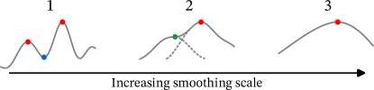
Figure 1: Typical density field around a critical event in 1D. From left to right: 1. We see two distinct objects (in red), separated by a minimum (in blue) in the density field. 2. The critical event occurs (in green), but the density profile still shows two different objects (highlighted with dashed lines). 3. The merger has completed and there remains only one object (in red).

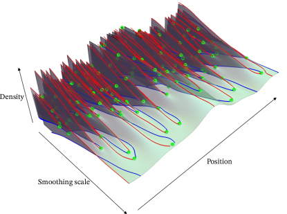
Figure 2: Representation of the smoothing of a 1D Gaussian random field representing density fluctuations in the primordial universe. Red lines are maxima of the field, blue lines are the minima. Green points are critical events, where a minimum/maximum pair meets and annihilates itself. By counting how many critical events there are in the vicinity of a peak line, one can count the number of subhalos merging into the corresponding halo.

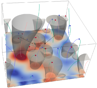
Figure 3: Visualisation of the action of gaussian smoothing on the critical events of a 2D field. The vertical axis is the smoothing scale, increasing upwards. The horizontal cross-section is a 2D space. The various vertical lines represent the tracks of extrema positions (maxima in pink, minima in blue, saddles in green) as one changes the field smoothing. The red and blue squares represent the corresponding critical events (in red are points of peak–saddle and in blue that of minima-saddle coalescence). The gray cones shows the volume within some fraction of the smoothing scale (here chosen arbitrarily to be 1.2 times the smoothing scale) around each maxima track, which contain all the past physical history of a given peak. This paper aims to characterise these cones and the properties of the critical events within them so as to compute major merger rates as a function of final halo mass.

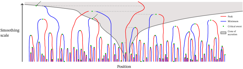
Figure 4: Our model associates peaks (in red) to halos, and critical events (in green) to mergers as a function of smoothing scale $R$ which encodes mass evolution. Critical events correspond to the coalescence of a peak with a minimum (in blue). We count any critical event directly connected to the central peak (i.e. not separated by another minimum, shown here as gray dashed lines) as a merger. Here, this definition would give use 6 mergers into the central peak. Alternatively, we can estimate this number by counting the number of critical events within some fraction of the smoothing scale $\alpha R$ (highlighted for one prominent peak in shaded gray). Here, $\alpha$ is chosen to recover to same count, but note that which events is selected may vary (as highlighted with the two arrows).

2 Analytical model of mergers per halo

2.1 Model of halo mergers: cone of influence of a halo

The starting point of our approach is the peak picture (Bardeen et al., 1986). In this framework, peaks in the linear density field are the seeds for the formation of halos. We rely on the proposition that the overdensity $\delta(R)$ of a given peak smoothed at scale $R$ can be mapped to a formation redshift $z$, using the spherical collapse model, $\delta(R_{\mathrm{TH}})D(z)=\delta_{\mathrm{c}}$, where $\delta_{\mathrm{c}}=1.686$ is the critical density, $D(z)$ is the growing mode of perturbations and $R_{\mathrm{TH}}$ is the top-hat scale. The mass of the halo formed at this time is inferred from the top-hat window scale, $M=\bar{\rho}_{\mathrm{m}}\frac{4}{3}\pi R_{\mathrm{TH}}^{3}$.

While the peak-patch theory provides useful insight in the origin of halos of a given mass at a given time, it becomes singular during mergers. Indeed, by construction, the merging halo disappears into the larger one together with its corresponding peak. Here, we instead rely on the analysis of the geometry of the initial linear density field in $N$+1D, where $N$ is the dimension of the initial Lagrangian space and the extra dimension is the smoothing scale. At each smoothing scale, we can formally define critical points (peaks, saddles and minima) following Bardeen et al. (1986). As smoothing increases, some of these critical points eventually disappear when their corresponding halo (for peaks) merge together. This approach allows to capture mergers in space-time from an analysis of the initial conditions in position-smoothing scale employing the critical event theory (Hanami, 2001; Cadiou et al., 2020), where critical events of coalescence between peaks and saddle points serve as proxies for merger events. The process is sketched in Fig. 1 and illustrated in 1+1D in Fig. 2.

Let us track the Lagrangian history with decreasing smoothing of one peak first identified at a smoothing scale $R_{0}$ and position $x_{\mathrm{pk}}(R_{0})$. Critical event theory relies on the use of Gaussian filters, so that, to assign mass to halos, we need to match the Gaussian and Top-Hat smoothing scales, $R$ and $R_{\mathrm{TH}}$. The criteria of equal mass encompassed by the filter gives $R_{\mathrm{TH}}\approx 1.56R$. At $R_{0}$ the peak describes a halo that has collected its mass from a spherical cross-section of $N$+1D space of volume $\propto R_{0}^{3}$; we can call this sphere a Lagrangian patch of the halo. At smaller $R$, the Lagrangian position of a peak changed to $x_{\mathrm{pk}}(R)$ and the volume of its Lagrangian patch decreased to $\propto R^{3}$. The history of the peak in the $N$+1D space, including mass accumulation, now consists of its trajectory $x_{\mathrm{pk}}(R)$ and a cone of cross-section $\sim R^{3}$ around it as shown in Fig. 3 for 2+1D example.

A critical event marks the end of a trajectory of a peak that disappeared when its scale reached $R_{\mathrm{ce}}$ and is absorbed into a surviving peak. Counting all critical events within a $N+1$D straight cylinder with spatial cross-section of radius $R_{0}$ around the final surviving peak position $x_{\mathrm{pk}}(R_{0})$ will give the number of all mergers that ever happened within this peak Lagrangian patch. For instance, if two small halos have merged together before merging with a larger halo, that would count as two events. However, we are interested in counting only the last direct merger event that brought the combined mass of the two small halos into the main one. Physical intuition tells us that to count only those, we need to count critical events within the history cone of the peak mass accumulation. Indeed, the Lagrangian patch of the peak grows in size by absorbing the layers along its boundary, and if that layer contains a critical event, it is a direct merger.

In 1+1D, as illustrated in Fig. 4, direct mergers correspond to critical events (green points) that are not separated by any intervening peak (red) lines from the main peak. In $(N+1)$D, this is generalized by only counting a critical event as a direct merger if, at fixed smoothing $R=R_{\mathrm{ce}}$, it is connected to the main peak in $N$D space by a filamentary ridge with no other peak in-between.

Fig. 4 confirms that indeed, most critical events that are directly connected to the main peak lie within a “cone of influence” whose size is $\alpha R$, where $\alpha$ is between 2 and 4, and vice versa this cone contains almost exclusively only the direct mergers. Counting critical events within the “influence cone” of the peak that can be shown to contribute to the mass and spin growth of this surviving halo is the main analytical tool of this paper.

The evolution of a halo in smoothing direction tells us directly its history in terms of mass accumulation, as $M\propto R^{3}$. That is, we can describe what happened with the halo as its mass increased, say, 10 fold. In the next section we apply this picture to count merger events.

2.2 Number of major merger events within a mass range

Here and in the following, we are interested in counting the number of objects that directly merged into an object of final mass $M_{0}$ as its mass grew from $f^{3}M_{0}$ to $M_{0}$, where $f<1$. Since smoothing scale maps directly onto mass, this amounts to counting the number of critical events between two scales $R_{0}\propto\sqrt[3]{M_{0}}$ and $R_{1}\propto f\sqrt[3]{M_{0}}$.

Let us now count direct major mergers that we define as mergers with satellites that bring at least $f^{3}M_{0}$ mass in the merger event, with $f<1$. First note that we define here the mass ratio with respect to the final mass of the peak at a fixed time, rather than at the time of the merger. The number of such mergers, as halo grew from $f^{3}M_{0}$ to $M_{0}$, is given by the number of critical event in the section of the cone of influence of the halo which is contained between $fR_{0}$ and $R_{0}$. It can be obtained with the following integral

$$N_{\mathrm{merger}}=\int_{fR_{0}}^{R_{0}}\differential{R}\int_{0}^{\alpha R}\differential[3]{r}n_{\mathrm{ce}}(R,{\bf\it r}),$$ (1)

where $n_{\mathrm{ce}}(R,{\bf\it r})$ is the number density of critical events at the point $(R,{\bf\it r})$, in the extended 4D space of positions–smoothing scale. Note that in the above formula we are able to avoid the dependence on the past trajectory $x_{\mathrm{pk}}(R)$ of the halo, by treating each slab of constant $R$ independently, and by evaluating the radial distance $r$ to the critical event found of at $R$ from the main peak position, $x_{\mathrm{pk}}(R)$, defined at the same smoothing.

As a first estimate, let us approximate $N_{\mathrm{merger}}$ by taking the density of the critical events inside the cone of influence to be equal to its mean value. Thus, we first neglect any spatial correlation between the existence of a peak (corresponding to the surviving object in a merger) and the critical event (corresponding to the absorbed object in a merger). In Cadiou et al. (2020), we determined that the average density of critical events that correspond to peak mergers is given by

$$\bar{n}_{\mathrm{ce}}=\frac{R}{R_{*}^{5}}\frac{1-\tilde{\gamma}^{2}}{\tilde{\gamma}^{2}}\frac{29\sqrt{15}-18\sqrt{10}}{600\pi^{2}}\,,$$ (2)

where the spectral scale $R_{*}$ and parameter $\tilde{\gamma}$ are given in Appendix A, together with other parameters that characterize the statistics of a density field. Note that $R_{*}\propto R$, so the number density of critical events scales as $n_{\mathrm{ce}}\propto R^{-4}$. The cubic part of this dependence, $R^{-3}$, reflects the decrease of spatial density of critical points with increasing smoothing scale; the additional scaling, $R^{-1}$, reflects that the frequency of critical events is uniform in $\log R$.

Assuming a power-law density spectrum with index $n_{\mathrm{s}}$ and Gaussian filter, equation 2 gives

$$\bar{n}_{\mathrm{ce}}=0.0094\left(\frac{5+n_{\mathrm{s}}}{2}\right)^{3/2}R^{-4}\,.$$ (3)

Using this mean value $\bar{n}_{\mathrm{ce}}$ for critical density in equation 1 gives us a first rough, but telling estimate of the merger number that a typical halo experiences

$$N_{\mathrm{merger}}\approx 0.039(-\ln f)\left(\frac{5+n_{\mathrm{s}}}{2}\right)^{3/2}\alpha^{3}.$$ (4)

The final results depends on the specific value of $f$ and $\alpha$. The value of the fraction $f$ controls down to which mass ratio mergers should be included and has thus a straightforward physical interpretation. The parameter $\alpha$ controls the opening of the cone of influence around the peak from which critical events should be considered as direct mergers.

Using equation 4 with $n_{\mathrm{s}}=-2$, which corresponds to the typical slope of a $\Lambda$CDM power-spectrum at scales ranging from Milky-Way like systems to clusters, we can count the number of direct mergers with mass ratio larger than 1:10 ($f=1/\sqrt[3]{10}$). Let us consider two cases. For instance, if we count only critical events within the halo Top-Hat Lagrangian radius, $\alpha=R_{\mathrm{TH}}/R\approx 1.56$, we find $N_{\mathrm{merger}}\approx 0.2$. However, as will bear out in the analysis presented in the next sections, a more sensible choice is to extend the opening angle to twice that ratio $\alpha=2R_{\mathrm{TH}}/R\approx 3.1$ (two mass spheres of the surviving and merging peaks are touching at the scale of critical event). We then find $N_{\mathrm{merger}}\approx 1.7$. Overall, we see that the number of direct major mergers that a halo experiences while increasing its mass tenfold is small, of the order of one or two. For scale invariant history, each decade of mass accumulation contributes similar number of mergers, so a cluster that grew from a galactic-scale protocluster thousand-fold in mass ($f=1/\sqrt[3]{1000}$), did it having experienced $N_{\mathrm{merger}}\approx 5$ major mergers. These conclusions follow directly from first principles, while studying the structure of the initial density field .

2.3 Accounting for rarity and clustering

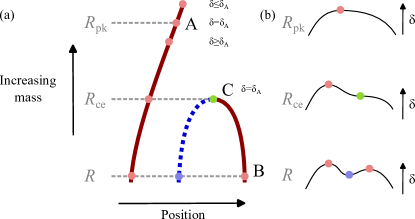
Figure 5: Panel a) shows the tracks of two peaks (red) and a saddle point (blue) of the density field as a function of smoothing scale $R$ in 1+1D space. Panel b) shows field profile at three smoothing scales. At smoothing scale $R_{0}$, the peaks and saddle points are distinct. At smoothing $R_{\mathrm{ce}}$, one peak and a saddle point create a critical event C, after each only one peak survives to larger smoothing scales. The merging of peaks is completed at the scale $R_{\mathrm{pk}}$ when the overdensity of the surviving peak, now at point A, is equal to the overdensity of the critical event $\delta_{\mathrm{C}}$ and thus can be viewed as reaching the threshold $\delta_{\mathrm{c}}$ for halo formation at the same time. We can then interpret the critical event as a merger with mass ratio $M_{\mathrm{A}}/M_{\mathrm{C}}=(R_{\mathrm{ce}}/R_{\mathrm{pk}})^{3}$ at a redshift corresponding to $D(z)=\delta_{\mathrm{c}}/\delta_{\mathrm{A}}$.

Let us now refine our model so as to define $\alpha$ more rigorously by i) requiring the merging object to have gravitationally collapsed before it merges and by ii) taking into account the correlations between the central halo peak and the merger critical events.

Let us therefore consider the number density of critical events of given height $\nu$ as a function of their distance $r$ to a central peak, both defined at the same smoothing scale $R$

$$n_{\mathrm{ce}|\mathrm{pk}}(\nu,R,r)=\bar{n}_{\mathrm{ce}}(R)C(\nu,\gamma)\left(1+\xi_{\mathrm{ce},\mathrm{pk}}(\nu,R,r)\right)\,,$$ (5)

where $C$ is the distribution function, $\int_{-\infty}^{\infty}C(\nu,\gamma)\differential{\nu}=1$, of critical events in overdensity and is given by the analytical formula in Appendix D along with a useful Gaussian approximation. The clustering of critical events in the peak neighbourhood is described by the peak-critical event correlation function on a slice of fixed $R$, $\xi_{\mathrm{ce},\mathrm{pk}}(\nu,R,r)$. The composite index $\mathrm{pk}$ refers to any peak parameters that may be specified as a condition. Our goal is to determine what range of $\nu$ and what extent of $r$ one needs to consider to count halos merging into a surviving halo with a particular $\nu_{\mathrm{pk}}$.

2.3.1 Heights of critical events

To establish the range of critical event heights that describe mergers of real halos, we rely on the spherical collapse approximation to map the peak overdensity to its gravitational collapse time. We consider a physical halo at redshift $z$ to be described by a peak at the Top-Hat scale $R_{\mathrm{pk}}$ such that $\delta_{\mathrm{pk}}(R_{\mathrm{pk}})=\delta_{\rm c}/D(z)$, where $\delta_{\rm c}$ is the critical overdensity for collapse model and $D(z)$ is the linear growing mode value at redshift $z$. Thus, a critical event found at smoothing $R_{\mathrm{ce}}$ describes the merger of a satellite halo of scale $R_{\mathrm{ce}}$ into the main peak at scale $R_{\mathrm{pk}}$ that corresponds to the same redshift, i.e such that $\delta_{\mathrm{ce}}(R_{\mathrm{ce}})=\delta_{\mathrm{pk}}(R_{\mathrm{pk}})=\delta_{\rm c}/D(z)$. The situation is demonstrated in Fig. 5. The ratio of scales and, correspondingly, masses of the two merging halos is therefore determined by the condition of equal overdensities at the time of merger.

Let us now consider a peak that has reached a scale $R_{0}$ and that experienced a merger in its past when its scale was $R_{\mathrm{pk}}$, $R_{\mathrm{pk}}\leq R_{0}$. Requiring that, at the time of the merger, the surviving peak’s scale (mass) is larger than that of the satellite sets the relation $R_{0}\geq R_{\mathrm{pk}}\geq R_{\mathrm{ce}}$ or, conversely, $\sigma(R_{0})\leq\sigma(R_{\mathrm{pk}})\leq\sigma(R_{\mathrm{ce}}$). From which it follows that the rarity of the relevant critical events at scale $R_{\mathrm{ce}}$,

$$\nu=\frac{\delta_{\mathrm{ce}}(R_{\mathrm{ce}})}{\sigma(R_{\mathrm{ce}})}=\frac{\delta_{\mathrm{pk}}(R_{\mathrm{pk}})}{\sigma(R_{\mathrm{ce}})}=\nu_{\mathrm{pk}}\frac{\sigma(R_{\mathrm{pk}})}{\sigma(R_{\mathrm{ce}})}$$ (6)

is within the range

$$\nu_{\mathrm{pk}}\frac{\sigma(R_{0})}{\sigma(R_{\mathrm{ce}})}\leq\nu\leq\nu_{\mathrm{pk}}.$$ (7)

The lower bound corresponds to mergers that have completed at the very last moment, $R_{\mathrm{pk}}=R_{0}$. The upper bound is achieved for mergers of two equal mass objects, $R_{\mathrm{pk}}=R_{\mathrm{ce}}$.

To obtain the total number of merger events in a halo history we now integrate the conditional event density in equation 5 over the physically relevant range of heights from equation 7, i.e.

$$N_{\mathrm{merger}}(\nu_{\mathrm{pk}})=\\ \int_{fR_{0}}^{R_{0}}\differential{R}\int_{0}^{\infty}4\pi r^{2}\differential{r}\int_{\nu_{\mathrm{pk}}\frac{\sigma(R_{0})}{\sigma(R)}}^{\nu_{\mathrm{pk}}}\differential{\nu}n_{\mathrm{ce}|\mathrm{pk}}(\nu,R,r).$$ (8)

2.3.2 Clustering of critical events around peaks

Ultimately, the conditional event density $n_{\mathrm{ce}|\mathrm{pk}}$ should include only critical events that will directly merge with the peak in the constraint; this would make the density of critical events go to zero $n_{\mathrm{ce}|\mathrm{pk}}(\nu,R,r)\to 0$ far from the peak, i.e. when $r\to\infty$. While we cannot implement this condition analytically (as it is non local), we can measure $n_{\mathrm{ce}|\mathrm{pk}}(\nu,R,r)$ numerically, as will be done in the upcoming Section 3. We can however approximate the conditional density ab initio by relaxing the conditions that the peak is linked to the critical event to obtain $\widetilde{n}_{\mathrm{ce}|\mathrm{pk}}$ given by

$$\widetilde{n}_{\mathrm{ce}|\mathrm{pk}}(\nu,R,r)\equiv\frac{\langle\operatorname{Peak}({\bf\it x})\operatorname{Event}({\bf\it y})\rangle}{\langle\operatorname{Peak}({\bf\it x})\rangle}\,,$$ (9)

using formally straightforward analytical calculations of critical event – peak correlations, as described in Appendix B. Here, ${\bf\it x}$ and ${\bf\it y}$ are the random vectors containing the density and its successive derivatives at the location of the peak and the critical event, respectively and ‘$\operatorname{Peak}$’ and ‘$\operatorname{Event}$’ enforce the peak and critical event conditions respectively. We can expect $\widetilde{n}_{\mathrm{ce}|\mathrm{pk}}$ to track the exact $n_{\mathrm{ce}|\mathrm{pk}}$ up to several smoothing length distance from the peak, but further away from the peak it just describes the mean unconstrained density of critical events: $\widetilde{n}_{\mathrm{ce}|\mathrm{pk}}(\nu,R,r)\to\bar{n}_{\mathrm{ce}}(R)C(\nu)$ as $r\to\infty$. Therefore, in this approximation the question of where to truncate the integration over the peak neighbourhood remains and we have

$$N_{\mathrm{merger}}(\nu_{\mathrm{pk}})\approx\\ \int_{fR_{0}}^{R_{0}}\differential{R}\int_{0}^{\alpha R}4\pi r^{2}\differential{r}\int_{\nu_{\mathrm{pk}}\frac{\sigma(R_{0})}{\sigma(R)}}^{\nu_{\mathrm{pk}}}\differential{\nu}\widetilde{n}_{\mathrm{ce}|\mathrm{pk}}(\nu,R,r).$$ (10)

For scale-free spectra, introducing the dimensionless ratios $u=r/R$ and $w=R/R_{0}$ and changing the order of integration, equation 8 can be written as

$$N_{\mathrm{merger}}(\nu_{\mathrm{pk}}) =\int_{f}^{1}\frac{\differential{w}}{w}\int_{0}^{\infty}\differential{u}\frac{\differential[2]{N_{\mathrm{ce}|\mathrm{pk}}}}{\differential u\;\differential\ln w},$$

$$\frac{\differential[2]{N_{\mathrm{ce}|\mathrm{pk}}}}{\differential u\;\differential\ln w} \equiv 4\pi u^{2}\int_{\nu_{\mathrm{pk}}w^{(n+3)/2}}^{\nu_{\mathrm{pk}}}\!\!\!\!\!\differential{\nu}w^{4}{n}_{\mathrm{ce}|\mathrm{pk}}(\nu,w,u)\,,$$ (11)

where we note that the differential event count per logarithm of smoothing scales has only a dependence on the smoothing scale $w$ via the bounds of the height integration, since for power-law spectra $w^{4}n_{\mathrm{ce}|\mathrm{pk}}(w)$ is $w$-independent.

In Fig. 6, we plot the differential version of equation 11 per radial spatial shell, integrated over $\nu$ in the range $0.681\nu_{\mathrm{pk}}\leq\nu\leq\nu_{\mathrm{pk}}$ which corresponds to $(R/R_{0})^{3}=1/10$ for $n=-2$ power-law spectrum. Fig. 6 shows that critical events are indeed preferentially clustered at distances $\sim 3R$ from a peak. It is natural to interpret this distance as the boundary of the cone influence of the peak, with more distant critical events constituting “the field” of events that are not directly merging into the peak. Thus, the computation of the correlation function supports choosing $\alpha\approx 3$ in the estimate of equation 4, i.e. qualitatively double the value of $R_{\mathrm{TH}}$. Note also that the probability of a critical event to be found close to a peak is suppressed, which corresponds to an exclusion from the interior of the peak’s cone of influence, as was qualitatively observed in Fig. 4.

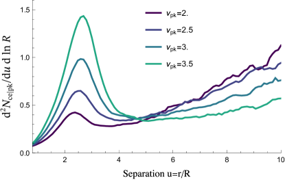
Figure 6: Integration of the analytical expression of the clustering of critical events around peaks, equation 11, for different values of $\nu_{\mathrm{pk}}$. Here $\nu_{\mathrm{ce}}$ is integrated from $0.681\nu_{\mathrm{pk}}$ to $\nu_{\mathrm{pk}}$, with power spectrum $n=-2$ and smoothing ratio $R_{\mathrm{pk}}/R_{\mathrm{ce}}=0.95$. We detail the method used to compute this graph in Section C.1. Rarer peaks have a stronger excess of events in their vicinity, which mirrors the known Kaiser bias (Kaiser, 1984).

3 Numerical integration of mergers

We will now rely on a numerical approach to study the properties of the mergers a given halo undergoes through the properties of critical events that are absorbed by the peak representing the halo. The main numerical step is the identification of critical event–peak pairs that mark specific mergers. This in turn involves the identification in the initial field at a sequence of smoothing scales of connected peak–saddle–peak triplets that describe filamentary link between the merging peaks. At a particular smoothing scale, the saddle and one of the peak of a given triplet merge into a critical event, while the remaining peak is a surviving halo. Such triplets are identified with DisPerse (Sousbie et al., 2009) that performs Morse complex analysis of the random density field. We perform the analysis on an ensemble of scale-free Gaussian realizations of initial density fields.

3.1 Number of mergers per peak line

We identify proto-events as close-to-zero persistence-pairs of peaks and filament-saddles, and we study here their clustering relative to a given peak. We proceed as follows: we generate 430 scale-invariant gaussian random fields of size $256^{3}$ with a power law power spectrum with spectral index $n=-2$ . We smooth each field with a Gaussian filter over multiples of a given smoothing scale. Here we choose $R=1.1^{k}\ $\mathrm{p}\mathrm{i}\mathrm{x}\mathrm{e}\mathrm{l}$$ with $k$ running from 15 to 49. Each smoothing step corresponds to 33% increase in the mass associated with the smoothing scale, and 8 steps give the mass increasing approximately 10-fold. The skeleton is identified at each scale using DisPerse (Sousbie et al., 2009) with a persistence threshold of $1\text{\,}\mathrm{\char 37\relax}$ of the RMS of the smoothed fields. We also measure at each critical point the value of the gravitational acceleration. We detect events by following each pair of peak and saddle from one smoothing scale to the next one. Each pair either survives at the next smoothing scale, or it disappears at a critical event. In the latter case, we define the position of the critical event as the middle point of the pair at the largest smoothing scale where it survived. Given that DisPerse (Sousbie, 2011) stores for each saddle the two maxima it is paired with, we can therefore associate the critical event to the one peak that is not involved in the event.

Using this data, we can now study the clustering of critical events around peaks. In Fig. 7, we show the ratio of the number of critical events per logarithmic smoothing scale bin per unit distance to the number of peaks at the same scale and at the same rarity. Critical events are counted in the interval of rarity $0.681\;\nu_{\mathrm{pk}}\leq\nu_{\mathrm{ce}}\leq\nu_{\mathrm{pk}}$. This range corresponds to the smallest scale cross section of the influence cone if we count major mergers of a peak that that grows ten times in the process, i.e. $R_{\mathrm{ce}}=1/\sqrt[3]{10}R_{0}$ in equation 8. Note that our quantity differs from two-point correlations functions in which one would compute the distance between any critical event and any peak, as was done in the previous section (Fig. 6). Here, each critical event only contributes to the density at a single distance to its associated peak, and we thus expect the signal to drop to zero at infinite separation, since the probability for a critical event to be associated with a peak far away vanishes.

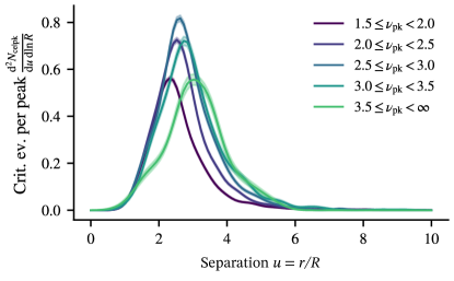
Figure 7: The radial number density of topologically linked critical event per peak as a function of distance to the peak on a slice of constant $R$ and per logarithmic bin in smoothing scale (see the text for details of how critical events are identified and paired to a peak). Critical events are preferentially clustered at $r\sim 2.5-3.5R$, depending on rarity. When compared to Fig. 6, the rarer peaks have relatively less connected events, suggesting that their satellites would have merged together before merging into the central object.

Should the critical events be randomly distributed, their number per linear $\differential r$ would grow as $r^{2}$. Instead, in Fig. 7 we find an exclusion zone at small separations, an excess probability at $r/R\sim 2-3$ and a cut-off at large separations as a consequence of our requirement for the critical event to be paired to a peak.

We integrate the curves in Fig. 7 and report the mean number of critical events per peak per logarithmic smoothing bin in Table 1. All the effects accounted for in our numerical analysis give just $\approx 40\%$ lower values in Table 1 relative to equation 4 (per $\ln f$) with $\alpha=3.1$. This shows that the two main corrections to the naive uniform density estimate — the restriction to only collapsed satellite halos (Section 2.3.1) on the one hand, and an attraction of critical events of similar heights towards the peak influence zone (Section 2.3.2) on the other hand — compensate each other to a large extent.

As a function of peak rarity $\nu_{\mathrm{pk}}$, the mean number of critical events per peak in a constant $R$ slab first increases up to $\nu_{\mathrm{pk}}\approx 3$ before decreasing. It is fairly flat in the range $\nu_{\mathrm{pk}}=2.5-3.5$, where most of the physical halos are, which argues for taking $\alpha$ parameter independent on $\nu_{\mathrm{pk}}$ if one uses the rough estimate as the global mean density of events times effective volume as in equation 4, Section 2.2.

Table 1: Number of critical event per peak, both being measured at the same scale, per logarithmic bin of smoothing scale, as a function of the rarity of the peak.

$\nu_{\mathrm{pk}}$ range	$[1.5,2.0[$	$[2.0,2.5[$	$[2.5,3.0[$	$[3.0,3.5[$	$[3.5,\infty[$
$\dfrac{\differential{N_{\mathrm{ce}|\mathrm{pk}}}}{\differential{\ln R}}$	0.90	1.20	1.40	1.42	1.27

So far, we have only studied properties of peaks and critical events at the same scale, using the defining equation 7 to implicitly perform a multi-scale analysis. We can however track peaks from one slab of smoothing scale to another to build peak lines and associate them to critical events. This generalizes the procedure sketched on Fig. 4 in 3+1D. For each peak with mass $M_{\mathrm{pk}}$, we follow its peak line to find all associated critical events with a mass $M_{\mathrm{pk}}\geq M_{\mathrm{ce}}\geq M_{\mathrm{pk}}/10$ that have $\delta_{\mathrm{ce}}(R_{\mathrm{ce}})\geq\delta_{\mathrm{pk}}(R_{\mathrm{pk}})$ where $R_{\mathrm{ce}}$ and $R_{\mathrm{pk}}$ are now different. We only retain peaks that exist at scales $R_{\mathrm{pk}}\geq R_{\mathrm{min}}\sqrt[3]{10}$ to ensure that we do not miss critical events below our smallest scale.

Given our numerical sample, we are now in a position to study the distribution of the number of merger per peak, which we show on Fig. 8. This measurement differs from the value one would obtain by taking Table 1 multiplied by the logarithm of the range of scales. Indeed, we account here for the decrease in the number of relevant satellites as their mass approaches the final peak mass. We also obtain our measurement by computing the number of mergers per surviving peak at the scale $M_{\mathrm{pk}}$. Compared to that, in Table 1, we give the value per any peak at $1/10M_{\mathrm{pk}}$ scale, irrespective of whether and how long it would survive at the further smoothing scales. We find that the dependence of the number of merger with peak height is weak, with a mean number of mergers varying between 1.8 and 2. This shows that in the language of effective influence cone radius of equation 4, $\alpha=2R_{\mathrm{TH}}/R=3.1$ is a very good proposition.

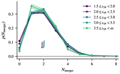
Figure 8: Distribution of the number of major mergers for peaks in different rarity bins, as labelled. The mean number of major mergers increases from $1.8$ for low-$\nu$ peaks to $2$ for high-$\nu$ peaks and is graphically represented with vertical lines with tilted caps for readability.

3.2 Orbital spin parameter of mergers

Let us now define the spin parameter of an event at scale $R_{\mathrm{ce}}$ relative to a peak of rarity $\nu$ at scale $R_{\mathrm{pk}}$ as

$$\lambda(\nu)=\frac{R_{\mathrm{ce}}^{3}}{R_{\mathrm{pk}}^{3}}\frac{\left\langle\left|\mathbf{r}\times\nabla\psi\right|\,\middle|\,\nu\right\rangle}{\sqrt{2}R_{\mathrm{pk}}\sigma_{-1}(R_{\mathrm{pk}})}.$$ (12)

Here, we recall that $\sigma_{-1}$ is the variance of the gradient of the potential, whose definition is given in Appendix A. This definition reflects the spin definition of Bullock et al. (2001); it compares the orbital angular momentum brought by a merger to the angular momentum of a merger separated by a distance $R_{\mathrm{pk}}$ with a relative velocity $\sqrt{2}\sigma_{-1}$ with respect to the central peak, assuming that the velocities are well approximated by the Zel’dovich approximation. We show on Fig. 9 the distribution of the spin parameter $\lambda$. The sample consists of mergers with mass ratios greater or equal to 1:10 around rare peaks. In practice, we select $\nu_{\mathrm{pk}}>2.5;R_{\mathrm{pk}}/\sqrt[3]{10}\leq R_{\mathrm{ce}}\leq R_{\mathrm{pk}}$ and $\delta_{\mathrm{ce}}\geq\delta_{\mathrm{pk}}$. The distribution is roughly log-normal with a mean value of $\mu_{\lambda}\approx 0.048$ and a standard deviation of $\sigma_{\lambda}\approx 0.51$.

It is remarkable that our estimate for the orbital spin of mergers is found to be very close to the values measured in $N$-body simulations, which are on the order of 0.04 (see e.g. Bullock et al., 2001; Aubert et al., 2004; Bett et al., 2007; Danovich et al., 2015). Albeit simplistic, our model thus allows us to provide a natural explanation to the fact that mergers bring in a comparable amount of angular momentum to that of the full halo: gravitational tides alone (which is the only ingredient of our model) are able to funnel in a significant amount of angular momentum through mergers. This provides a theoretical motivation for the amplitude of the spin jumps during mergers employed in semi-analytical models (see e.g. Vitvitska et al., 2002; Benson et al., 2020).

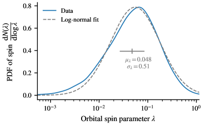
Figure 9: Merging objects bring in orbital spin; we quantify here its distribution. The distribution ressembles a log-normal distribution with parameters $\mu_{\lambda}\approx 0.048$ and $\sigma_{\lambda}\approx 0.51$; the distribution resembles its $N$-body counterpart.

3.3 Mass distribution of mergers

Finally, we compute the mass distribution of mergers as well as their density. The goal here is to obtain the distribution of the time and mass ratios of the mergers. In order to build the distribution of the mass ratio, we track peaks over multiple decades of smoothing scales (i.e. mass). Since the number density of peaks evolves as $R_{\mathrm{pk}}^{-3}$, the sample size quickly decreases with smoothing scale; we select here peaks that exist at a scale larger than $R_{\mathrm{min}}\sqrt[3]{100}\approx 4.6R_{\mathrm{min}}$. The practical consequence is that our sample is only complete over two decades in mass ratio. We also only retain rare peaks that have $\nu_{\mathrm{pk}}>2.5$. Let us then estimate the time of the merger as follows: we associate to both the peak and the critical event a time $t_{\mathrm{pk}}$ and $t_{\mathrm{ce}}$ respectively, using $\delta=\delta_{\mathrm{c}}/D(z)$. Note that some of the selected peaks will have collapsed by $z=0$ while other will in the distant future. In order to aggregate peaks collapsing at different times, we compute the lookback time of the merger relative to the collapse time of the peak $\Delta=(t_{\mathrm{pk}}-t_{\mathrm{ce}})/t_{\mathrm{pk}}$. We estimate the distribution of mergers in lookback time-mass ratio space using a 2D kernel density estimation which we show in Fig. 10, top panel. As expected, the more massive the merger, the more recently it happened.

We then show on the bottom panel of Fig. 10 the cumulative distribution function of the merger time, for mass ratios larger than 1:10 as a function of peak height. We recover the trend found in $N$-body simulations that rarer halos have had more recent major mergers than lower mass ones. Cluster-like structures ($\nu_{\mathrm{pk}}\gtrapprox 3.5$) typically had $80\text{\,}\mathrm{\char 37\relax}$ of their mergers in the second half of their life (past $7\text{\,}\mathrm{G}\mathrm{y}\mathrm{r}$ for a cluster at $z=0$), and had half their mergers in the last third of their life (last $5\text{\,}\mathrm{G}\mathrm{y}\mathrm{r}$ for a cluster at $z=0$).

Our model reproduces qualitative trends observed in $N$-body simulations, namely that rarer peaks typically had their last major merger more recently than less rare ones.

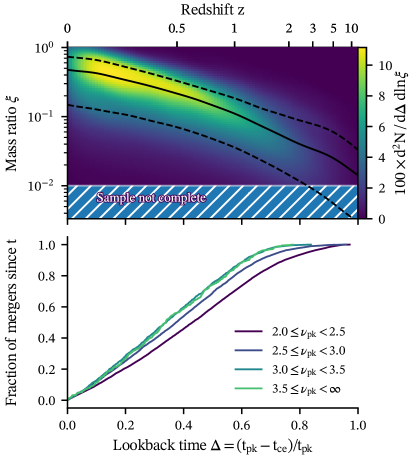
Figure 10: Top: distribution of the merger as a function of mass ratio and lookback time. We show the median with $68\text{\,}\mathrm{\char 37\relax}$ interval in black. The hashed area correspond to regions of the parameter space that may not be complete, see the text for details. Bottom: the corresponding fraction of major merger as a function of lookback time relative to the peak collapse time, for different peak heights. Rarer objects have had more recent mergers.

4 Conclusion and perspectives

We built a model of mergers from an analysis of the initial conditions of the Universe. Following the work of Hanami (2001); Cadiou et al. (2020), we relied on the clustering of critical events around peaks in the initial density field to study the properties of halo mergers. We started with a simple model that yields analytically tractable results, while further refinements presented in Section 3 allowed for more precise results at the cost of numerical integration.

We focussed here on the analysis of merger events that bring at least $10\text{\,}\mathrm{\char 37\relax}$ of the final mass of the main halo, which we refer to as ‘major mergers’. We however note that our approach can be extended to the analysis of minor mergers, which we leave for future work.

We first obtained a zero${}^{\text{th}}$-order analytical estimate of the mean number of mergers per decade in mass using the mean abundance of critical event per peak in Sections 2.1 and 2.2. Our results are consistent with halos having had one to two major mergers per relative decade of mass growth. We then refined our model in Section 2.3 by accounting for the timing of the collapse of the halos involved in a merger candidate; a critical event should only be counted as a merger if its two associated halos have collapsed before the merger happens. We showed this can be achieved semi-analytically by numerically computing the value of a cross correlation function, equation 10, that reveals that critical events cluster at 2-3 times the smoothing scale of the peak (Fig. 6).

Finally, in Section 3, we addressed the double-counting issue, whereupon a given critical event may be associated to several peaks, by uniquely associating each to the one peak it is topologically connected to. To that end, we relied on a multi-scale analysis of Gaussian random fields using computational topology to restrict ourselves to the study of peaks that, up to the critical event, form a persistent pairs. In this model, we found again that halos of different rarities undergo about 2 major mergers. By tracking peaks in position-smoothing scale and by associating critical events to them, we were able to provide numerically-cheap and easy-to-interpret data on the statistical properties of halo mergers. We found that mergers come from further away for rarer peaks (Fig. 7), but that the total number of major mergers only weakly depends on peak rarity (Fig. 8).

We then computed the gravitational tides at the location of the critical event to estimate the relative velocity of mergers and predict the orbital spin they bring in. We find that it has a log-normal distribution with a mean of $\mu_{\lambda}=0.048$ and $\sigma_{\lambda}=0.5$. These properties are remarkably close to the distribution of DM halo spins measured in hydrodynamical simulations ($\mu_{\lambda}=0.038$, $\sigma_{\lambda}=0.5$, Danovich et al., 2015). This suggests that our model captures the (statistical properties) of the orbital parameters of mergers, as is expected should they be driven by gravitational tides (Cadiou et al., 2021a, 2022). We also computed the distribution of the mass brought by mergers and their timing, which we found to be in qualitative agreement with results obtained in $N$-body simulations (Fakhouri et al., 2010).

While the aim of this model was not to compete with numerical simulations, it provides theoretical grounds to explain the properties of mergers observed in $N$-body simulations and efficient tools to predict their statistics and geometry ab initio. Our model could be improved with precision in mind, for example by taking into account deviations from spherical collapse under the effect of shears to improve our time assignments. It however reveals that the statistical properties of the merger tree of dark matter halo can be explained through a multi-scale analysis of these initial conditions.

4.1 Perspectives

Statistics involving successive mergers could potentially be built on top of our model by using critical event associated to the same peak line, for example to study the relative orientation of the orbital angular momentum of successive mergers. However, we found that such analysis was complicated by the fact that peak move with smoothing scale. Different definitions of the angular momentum (distance to the peak at the same scale, at the same density or for a fixed peak density) yielded qualitatively different results. This should be explored in future work.

The model built in this paper relied on a linear multi-scale analysis of the density field. This could be employed to provide control over the merger tree (timing of the merger, orientation) in numerical simulations through ‘genetic modifications’ of the initial field (Roth et al., 2016; Rey & Pontzen, 2018; Stopyra et al., 2021; Cadiou et al., 2021a, b). We also note that, as we did for tidal torque theory in Cadiou et al. (2022), such an approach would allow direct testing of the range of validity of the model.

This paper focussed on mergers of peaks corresponding to the relative clustering of peak-saddle events. One could extend the analysis to the relative clustering of saddle-saddle events to provide a theoretical explanation for which filaments merge with which, thus impacting their connectivity or their length (Galárraga-Espinosa et al., 2023). Conversely, extending the model to the relative clustering of saddle-void events (which wall disappears when?) is also of interest, as the later may impact spin flip, and is dual to void mergers, and as such could act as a cosmic probe for dark energy. One could compute the conditional merger rate subject to a larger-scale saddle-point as a proxy to the influence of the larger scale cosmic web, following both Musso et al. (2018) and Cadiou et al. (2020) to shed light on how the cosmic web drives galaxy assembly (Kraljic et al., 2018; Laigle et al., 2018; Hasan et al., 2023). Eventually, such theory could contribute to predicting the expected rate of starburst or AGN activity as a function of redshift and location in the cosmic web.

Author contributions

The main roles of the authors were, using the CRediT (Contribution Roles Taxonomy) system (https://authorservices.wiley.com/author-resources/Journal-Authors/open-access/credit.html):

CC: Conceptualization; formal analysis; investigation; methodology; software; writing – Original Draft Preparation; supervision. EPP: Investigation; software; writing – Review & Editing; Visualisation. CP: Conceptualization; formal analysis; methodology; software; investigation; writing – Review & Editing; supervision. DP: Conceptualization; formal analysis; methodology; writing – Review & Editing; validation; supervision.

Data availability

The data underlying this article will be shared on reasonable request to the corresponding author.

Appendix A Notations

Let us first introduce the dimensionless quantities for the density field, smoother over a scale $R$ by a filter function $W$

$$\delta({\bf\it r},R)=\int\frac{\differential[3]{k}}{(2\pi)^{3}}\delta({\bf\it k})W(kR)e^{i{\bf\it k}\cdot{\bf\it r}}.$$ (13)

We will consider the statistics of this field and its derivatives in this paper. For practical purposes, let us introduce

$$\sigma_{i}^{2}(R)\equiv\frac{1}{2\pi^{2}}\int_{0}^{\infty}\differential{k}k^{2}P(k)k^{2i}W^{2}(kR).$$ (14)

These are the variance of the density field $\langle\delta^{2}\rangle=\sigma_{0}^{2}$, of its first derivative $\langle\gradient{\delta}\cdot\gradient{\delta}\rangle=\sigma_{1}^{2}$, etc.

Following Pogosyan et al. (2009), let us introduce the characteristic scales of the field

$$R_{0}=\frac{\sigma_{0}}{\sigma_{1}},\quad R_{*}=\frac{\sigma_{1}}{\sigma_{2}},\quad\tilde{R}=\frac{\sigma_{2}}{\sigma_{3}}.$$ (15)

These scales are ordered as $R_{0}\geq R_{*}\geq\tilde{R}$. These are the typical separation between zero-crossing of the field, mean distance between extrema and mean distance between inflection points (Bardeen et al., 1986; Cadiou et al., 2020). Let us further define a set of spectral parameters that depend on the shape of the underlying power spectrum. Out of the three scales introduced above, two dimensionless ratios may be constructed that are intrinsic parameters of the theory

$$\gamma\equiv\frac{R_{*}}{R_{0}}=\frac{\sigma_{1}^{2}}{\sigma_{0}\sigma_{2}},\quad\tilde{\gamma}=\frac{\tilde{R}}{R_{*}}=\frac{\sigma_{2}^{2}}{\sigma_{1}\sigma_{3}}.$$ (16)

From a geometrical point of view, $\gamma$ specifies how frequently one encounters a maximum between two zero-crossings of the field, while $\tilde{\gamma}$ describes, on average, how many inflection points there are between two extrema. These scales and scale ratios fully specify the correlations between the field and its derivative (up to third order) at the same point. For power-law power spectra of index $n$, $P(k)\propto k^{n}$, with Gaussian smoothing at the scale $R$ in 3D, we have $R_{0}=R\sqrt{2/(n+3)}$, $R_{*}=R\sqrt{2/(n+5)}$ and $\tilde{R}=R\sqrt{2/(n+7)}$ while $\gamma=\sqrt{(n+3)/(n+5)}$ and $\tilde{\gamma}=\sqrt{(n+5)/(n+7)}$.

Appendix B Peak-event correlation

In order to compute the number of merger in the vicinity of a peak, we need to compute the two-point correlation function between critical events and peaks. We achieve this by evaluating the joint density of peaks and critical events

$$n_{\mathrm{peak,ce}}=\left\langle\operatorname{Peak}({\bf\it x})\operatorname{Event}({\bf\it y})\right\rangle,$$ (17)

where the average is taken over all 30 random variables defining the peak and critical event field up to third derivative.

$$\operatorname{Peak}({\bf\it x})\equiv |J_{x}|\Theta_{\mathrm{H}}(-\mathrm{Tr}(\mathbf{H_{x}}))\Theta_{\mathrm{H}}({\textstyle\sum_{i}}\mathbf{H}_{x,i})\Theta_{\mathrm{H}}(\det\mathbf{H}_{x})$$

$$\times\delta_{\mathrm{D}}(x_{1})\delta_{\mathrm{D}}(x_{2})\delta_{\mathrm{D}}(x_{3})\delta_{\mathrm{D}}(x-\nu_{\mathrm{pk}}),$$ (18)

$$\operatorname{Event}({\bf\it y})\equiv |J_{y}|\Theta_{\mathrm{H}}(-\mathrm{Tr}(\mathbf{H_{y}}))\Theta_{\mathrm{H}}({\textstyle\sum_{i}}\mathbf{H}_{y,i})\delta_{\mathrm{D}}(\det\mathbf{H}_{y})$$

$$\times\delta_{\mathrm{D}}(y_{1})\delta_{\mathrm{D}}(y_{2})\delta_{\mathrm{D}}(y_{3})\delta_{\mathrm{D}}(y-\nu)\,.$$ (19)

Here, ${\bf\it x}=\{x,x_{1},\dots,x_{3},\mathbf{H}_{x},\mathbf{H}_{x,1},\dots,\mathbf{H}_{x,3}\}$ with $x$, $x_{i}$, $\mathbf{H}_{x}$, $\mathbf{H}_{x,i}$ the density, its gradient, its Hessian and the minors of its Hessian at the peak location and ${\bf\it y}=\{y,y_{1},\dots,y_{3},\mathbf{H}_{y},\mathbf{H}_{y,1},\dots,\mathbf{H}_{y,3}\}$ with $y$, $y_{i}$, $\mathbf{H}_{y}$ and $\mathbf{H}_{y,i}$ the density, its gradient, its Hessian and the minors of the Hessian at the critical event location. $|J_{x}|=|\det\mathbf{H}_{x}|$ and we provide an explicit formula for $|J_{y}|$ in equation 22. This expression is the rotationally-invariant equivalent of Equation 18 of Cadiou et al. (2020).

The two-point correlation function can then be found as

$$1+\xi_{\mathrm{ce},\mathrm{pk}}(\nu_{\mathrm{pk}},\nu,R,r)=\frac{\left\langle\operatorname{Peak}({\bf\it x})\operatorname{Event}({\bf\it y})\right\rangle}{\langle\operatorname{Peak}({\bf\it x})\rangle\langle\operatorname{Event}({\bf\it y})\rangle}.$$ (20)

Note that, compared to Cadiou et al. (2020), we cannot perform the integration in the frame of the Hessian here. Indeed, the numerator involves cross correlation between the peak and the critical event which break the rotational invariance assumption. While the exact integration cannot be carried out analytically, we can nonetheless compute it numerically.

Appendix C Covariance matrices

The covariance matrix of $x$, $x_{i}$, $x_{ij}$ is given by

$$C=\begin{pmatrix}1&0&0&0&\frac{\gamma}{3}&\frac{\gamma}{3}&\frac{\gamma}{3}&0&0&0\\ 0&\frac{1}{3}&0&0&0&0&0&0&0&0\\ 0&0&\frac{1}{3}&0&0&0&0&0&0&0\\ 0&0&0&\frac{1}{3}&0&0&0&0&0&0\\ \frac{\gamma}{3}&0&0&0&\frac{1}{5}&\frac{1}{15}&\frac{1}{15}&0&0&0\\ \frac{\gamma}{3}&0&0&0&\frac{1}{15}&\frac{1}{5}&\frac{1}{15}&0&0&0\\ \frac{\gamma}{3}&0&0&0&\frac{1}{15}&\frac{1}{15}&\frac{1}{5}&0&0&0\\ 0&0&0&0&0&0&0&\frac{1}{15}&0&0\\ 0&0&0&0&0&0&0&0&\frac{1}{15}&0\\ 0&0&0&0&0&0&0&0&0&\frac{1}{15}\\ \end{pmatrix}.$$ (21)

We provide in equation 22 the expression for the jacobian required to compute the number density of critical event in a covariant form. Here $x_{{ijk}}$ stands for the derivative of the field of order $i$ w.r.t. the first direction, $j$ w.r.t. the second direction and $k$ w.r.t. the third direction divided by the corresponding RMS defined by equation 14.

$$\frac{J_{y}}{R}=\det\mathbf{H}_{y}\times(\laplacian\gradient{y})\dotproduct\mathbf{H}_{y}^{-1}\dotproduct\gradient{\det\mathbf{H}_{y}}=\\ \bigg{[}y_{{}_{002}}y_{{}_{020}}y_{{}_{300}}\!-\!2y_{{}_{002}}y_{{}_{110}}y_{{}_{210}}\!+\!y_{{}_{002}}y_{{}_{120}}y_{{}_{200}}\!+\!2y_{{}_{011}}y_{{}_{101}}y_{{}_{210}}\!+\!2y_{{}_{011}}y_{{}_{110}}y_{{}_{201}}\!-\!2y_{{}_{011}}y_{{}_{111}}y_{{}_{200}}\!-\!y_{{}_{011}}^{2}y_{{}_{300}}\\ -2y_{{}_{020}}y_{{}_{101}}y_{{}_{201}}+y_{{}_{020}}y_{{}_{102}}y_{{}_{200}}+2y_{{}_{101}}y_{{}_{110}}y_{{}_{111}}-y_{{}_{101}}^{2}y_{{}_{120}}-y_{{}_{102}}y_{{}_{110}}^{2}\bigg{]}\\ \times\left((y_{{}_{012}}\!+\!y_{{}_{030}}\!+\!y_{{}_{210}})(y_{{}_{011}}y_{{}_{101}}\!-\!y_{{}_{002}}y_{{}_{110}})\!+\!(y_{{}_{002}}y_{{}_{020}}\!-\!y_{{}_{011}}^{2})(y_{{}_{102}}+y_{{}_{120}}\!+\!y_{{}_{300}})\!+\!(y_{{}_{003}}\!+\!y_{{}_{021}}\!+\!y_{{}_{201}})(y_{{}_{011}}y_{{}_{110}}\!-\!y_{{}_{020}}y_{{}_{101}})\right)+\\ \bigg{[}y_{{}_{002}}y_{{}_{020}}y_{{}_{210}}\!+\!y_{{}_{002}}y_{{}_{030}}y_{{}_{200}}\!-\!2y_{{}_{002}}y_{{}_{110}}y_{{}_{120}}\!-\!2y_{{}_{011}}y_{{}_{021}}y_{{}_{200}}\!+\!2y_{{}_{011}}y_{{}_{101}}y_{{}_{120}}\!+\!2y_{{}_{011}}y_{{}_{110}}y_{{}_{111}}\!-\!y_{{}_{011}}^{2}y_{{}_{210}}\\ \!+\!y_{{}_{012}}y_{{}_{020}}y_{{}_{200}}\!-\!y_{{}_{012}}y_{{}_{110}}^{2}\!-\!2y_{{}_{020}}y_{{}_{101}}y_{{}_{111}}\!+\!2y_{{}_{021}}y_{{}_{101}}y_{{}_{110}}\!-\!y_{{}_{030}}y_{{}_{101}}^{2}\bigg{]}\\ \times\left((y_{{}_{003}}+y_{{}_{021}}\!+\!y_{{}_{201}})(y_{{}_{020}}y_{{}_{200}}\!-\!y_{{}_{110}}^{2})\!+\!(y_{{}_{012}}\!+\!y_{{}_{030}}\!+\!y_{{}_{210}})(y_{{}_{101}}y_{{}_{110}}-y_{{}_{011}}y_{{}_{200}})+(y_{{}_{102}}\!+\!y_{{}_{120}}\!+\!y_{{}_{300}})(y_{{}_{011}}y_{{}_{110}}\!-\!y_{{}_{020}}y_{{}_{101}})\right)+\\ \bigg{[}y_{{}_{002}}y_{{}_{020}}y_{{}_{201}}\!+\!y_{{}_{002}}y_{{}_{021}}y_{{}_{200}}-2y_{{}_{002}}y_{{}_{110}}y_{{}_{111}}\!+\!y_{{}_{003}}y_{{}_{020}}y_{{}_{200}}\!-\!y_{{}_{003}}y_{{}_{110}}^{2}\!-\!2y_{{}_{011}}y_{{}_{012}}y_{{}_{200}}+2y_{{}_{011}}y_{{}_{101}}y_{{}_{111}}\\ \!+\!2y_{{}_{011}}y_{{}_{102}}y_{{}_{110}}\!-\!y_{{}_{011}}^{2}y_{{}_{201}}\!+\!2y_{{}_{012}}y_{{}_{101}}y_{{}_{110}}\!-\!2y_{{}_{020}}y_{{}_{101}}y_{{}_{102}}\!-\!y_{{}_{021}}y_{{}_{101}}^{2}\bigg{]}\\ \times\left((y_{{}_{102}}\!+\!y_{{}_{120}}\!+\!y_{{}_{300}})(y_{{}_{011}}y_{{}_{101}}\!-\!y_{{}_{002}}y_{{}_{110}})\!+\!(y_{{}_{002}}y_{{}_{200}}\!-\!y_{{}_{101}}^{2})(y_{{}_{012}}\!+\!y_{{}_{030}}\!+\!y_{{}_{210}})\!+\!(y_{{}_{003}}\!+\!y_{{}_{021}}\!+\!y_{{}_{201}})(y_{{}_{101}}y_{{}_{110}}\!-\!y_{{}_{011}}y_{{}_{200}})\right).$$ (22)

C.1 Numerical implementation

In this section, we describe how Fig. 6 was obtained. We used Monte-Carlo integration to numerically evaluate equation 11. The statistical distribution of the aforementioned field variables is regulated by its $30\times 30$ covariance matrix $\Sigma$, which we may compute symbolically for given separation distance $r$, smoothing scales $R_{\mathrm{pk}}$ and $R_{\mathrm{ce}}$ and spectral index $n_{\rm s}$. We aim to sample points following this distribution and evaluate the integrands of equation (B) to obtain the expectancies $\left\langle\operatorname{Peak}({\bf\it x})\operatorname{Event}({\bf\it y})\right\rangle$. Ideally we would like to evaluate the correlation function at identical smoothing scale. However, at equal smoothing scale and small separation, the covariance matrix becomes almost singular, resulting in unfavourable numerical artefacts plaguing the statistic of our result. To avoid this, we instead consider slightly different smoothing scales.

Of course, we can not naively do this directly, as $x,x_{i},y,y_{i},\det\mathbf{H_{y}}$ will almost never take the specific values that the Dirac deltas impose, and thus the integrands will almost always evaluate to zero. To circumvent this, we compute the distribution of the other field variables conditional to the Dirac deltas being satisfied, with two exceptions: as we will need to integrate $\nu_{\mathrm{pk}}$ over a range to recover equation 11 anyway, we replace $\delta_{\mathrm{D}}(y-\nu_{\mathrm{pk}})$ by $\Theta_{\mathrm{H}}(\nu_{\operatorname{peak}}^{\mathrm{max}}-y)\Theta_{\mathrm{H}}(y-\nu_{\operatorname{peak}}^{\mathrm{min}})$; furthermore, as $\det\mathbf{H_{y}}$ depends on several field variables, computing the conditional distribution is not easily feasible. We therefore replace $\delta_{\mathrm{D}}(\det\mathbf{H_{y}})$ by a ‘thick Dirac delta’, $\delta_{\mathrm{D}}^{\varepsilon}(\det\mathbf{H_{y}})=\frac{1}{2\epsilon}\Theta_{\mathrm{H}}(\varepsilon-\det\mathbf{H_{y}})\Theta_{\mathrm{H}}(\det\mathbf{H_{y}}+\varepsilon)$, for some small $\varepsilon$. The smaller $\varepsilon$ is, the thinner the Dirac delta and the more faithful it is to the original integral. However reducing $\varepsilon$ comes at the cost of reducing the convergence rate of the Monte-Carlo approach.

Once the conditional distribution is computed, we simply draw random points following this distribution and average the evaluation of the integrand on these points, which converges to the value of the integral. This allows to compute $\int_{\nu_{p}w}^{\nu_{p}}\mathrm{d}\nu\langle\operatorname{Peak}({\bf\it x})\operatorname{Event}({\bf\it y})\rangle$ and $\langle\operatorname{Peak}({\bf\it x})\rangle$, and results in Fig. 6. Practically, to obtain Fig. 6, we drew $2^{26}$ sample points. We used a smoothing ratio $R_{\mathrm{pk}}/R_{\mathrm{ce}}=0.95$ and a thick Dirac delta of size $\varepsilon=10^{-3}$.

Appendix D Event differential distribution

The differential density of critical events with different field values $\nu$ are derived in Cadiou et al. (2020) and read

$$n_{\mathrm{ce}}(\nu,R)=\frac{3R}{\tilde{R}^{2}R_{*}^{3}}\frac{1}{5}\left(\frac{3}{2\pi}\right)^{3/2}(1-\tilde{\gamma}^{2})\\ \sum_{i=5,6,9}c_{3,i}(\nu,\gamma)\exp\left(-\frac{\nu^{2}}{2(1-5\gamma^{2}/i)}\right),$$ (23)

where the full expressions for $c_{3,i}(\nu,\gamma)$ were given in equation (39) of Cadiou et al. (2020) Factorizing the mean density of the critical events, $\bar{n}_{\mathrm{ce}}$, in this expression such that

$$n_{\mathrm{ce}}(\nu,R)=\bar{n}_{\mathrm{ce}}C(\nu),\,\,\mathrm{with}\,\,\,\int_{-\infty}^{\infty}\differential{\nu}C(\nu)=1,$$ (24)

we introduce the normalized distribution of the events in height

$$C(\nu,\gamma)=\frac{18\sqrt{10\pi}}{29-6\sqrt{6}}\sum_{i=5,6,9}c_{3,i}(\nu,\gamma)\exp\left(-\frac{\nu^{2}}{2(1-5\gamma^{2}/i)}\right),$$

which depends on the power spectrum (and on the smoothing scale if the spectrum is not scale invariant) only through the spectral parameter $\gamma$. In Fig. 11, we show the behaviour of $C(\nu,\gamma)$ for several choices of $\gamma$ that correspond to the spectral slopes of interest $n=-2.5,-2,-1.5$, see equation 16. For comparison, the peak rarity distribution is represented as dashed lines. We see that critical events typically occur at lower $\nu$ than peaks, and are very rare for $\nu>3$.

We note that $C(\nu,\gamma)$ for $\nu<3$ can be approximated with an accuracy of better than ${10}^{-3}$ for $-2.5\leq n_{\mathrm{s}}\leq-1.5$ by a Gaussian with parameters

$$\tilde{C}(\nu,\gamma) =\frac{1}{\sqrt{2\pi}\tilde{\sigma}}\exp\left(-\frac{(\nu-\tilde{\mu})^{2}}{2\tilde{\sigma}^{2}}\right)\,,$$

$$\tilde{\mu} =1.546\gamma,\,\,\,\tilde{\sigma}=1-0.5084\gamma^{2}+0.04140\gamma.$$

We show on the top panel of Fig. 11 the residuals of this fit.

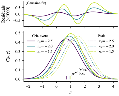
Figure 11: Normalized differential distribution of critical events in density rarity value for several value of spectral slope, as marked. The top panel shows the absolute residuals when fitting $C(\nu,\gamma)$ with a Gaussian function. Parameters of the Gaussian are provided in the text. We show the peak rarity distribution as thin dashed lines.

Appendix E Mean evolution of peak rarity

Let us predict the evolution of peak rarity with Gaussian smoothing. The value of the density field smoothed with a Gaussian window at position $x$ changes with window size $R$ according to the diffusion equation

$$\frac{\partial\delta({\bf\it r},R)}{\partial R}=R\Delta\delta({\bf\it r}_{\mathrm{pk}},R)\,.$$ (25)

If we are interested in the change of the peak value along the peak track ${\bf\it r}_{\mathrm{pk}}(R)$, we notice that the partial derivative $\partial/\partial R$ can be replaced by the full derivative, since at the peak $\gradient\delta=0$, thus

$$\frac{\differential{\delta({\bf\it r}_{\mathrm{pk}},R)}}{\differential{R}}=R\Delta\delta({\bf\it r}_{\mathrm{pk}},R)\,,$$ (26)

and for brevity we can now drop the reference to the position of the peak in the argument. In terms of rarity of the peak, $\nu(R)=\delta(R)/\sigma_{0}(R)$, the evolution equation becomes

$$\frac{\differential{\nu(R)}}{\differential\log R}=-\nu(R)\frac{\differential\log\sigma_{0}}{\differential\log R}+R^{2}\Delta\nu(R)\,.$$ (27)

The process of changing the peak height with smoothing is stochastic since the Laplacian of the field is a random quantity. However, to estimate the mean change, let us approximate the stochastic Laplacian by its conditional mean value given the height of the peak

$$\Delta\nu(R)\to\left\langle\Delta\nu(R)|\nu(R),\lambda_{i}<0\right\rangle,$$ (28)

where the last conditional inequality, written compactly in terms of the eigenvalues $\{\lambda_{i}\}_{i=1,\mathrm{D}}$ of the Hessian of the density, ensures that we are dealing with a maximum and not an arbitrary field point. In principle, one should also enforce the vanishing gradient of the field at peak position, but since the gradient of the field is uncorrelated with both the value and the second derivatives of the field at the same point, this condition is inconsequential for our problem.

Let us first evaluate the conditional mean in equation 28 in 1D, where the peak condition is just $\Delta\nu<0$. This gives us

$$\left\langle\Delta\nu|\nu,\Delta\nu<0\right\rangle=-\frac{\nu}{R_{0}^{2}}-\frac{1}{\zeta R_{0}^{2}}\sqrt{\frac{2}{\pi}}\frac{\exp\left(-\frac{\nu^{2}\zeta^{2}}{2}\right)}{1+\mathrm{erf}\left(\frac{\nu\zeta}{\sqrt{2}}\right)},$$ (29)

where $R_{0}$ is defined by equation 15, while $\zeta={\gamma}/{\sqrt{1-\gamma^{2}}}$ varies from zero at $\gamma=0$, to infinity at $\gamma=1$. The first term in equation 29 is the general conditional response of the Laplacian to the field value, while the second correction comes from restricting the field to be at the local maximum. For a Gaussian window function, we also have that ${\differential{\log\sigma_{0}}}/{\differential{R}}+{R}/{R_{0}^{2}}=0$ for any power spectrum. We can then obtain the (mean) evolution equation for the peak rarity

$$\frac{\differential{\nu(R)}}{\differential\log R}=-\frac{R^{2}}{\zeta R_{0}^{2}}\sqrt{\frac{2}{\pi}}\frac{\exp\left(-\frac{\nu^{2}\zeta^{2}}{2}\right)}{1+\mathrm{erf}\left(\frac{\nu\zeta}{\sqrt{2}}\right)},$$ (30)

where $R/R_{0}$ is a constant that depends on the power spectrum (cf Appendix A); it is equal to $\zeta$ for power-law spectra. Thus, the rarity of maxima is, on average, decreasing slowly with smoothing scale $R$. The decrease is less pronounced for rarer peaks and can be in first approximation neglected for $\nu\zeta>\sqrt{2}$.

For power law spectra in $D$ dimensions, $\zeta=\sqrt{(n+D)/2}$. We obtain a criterion for insignificant rarity drift for peaks rarer than $\nu>{2}/{\sqrt{n+D}}$. Note that this is based on generalizing the 1D result to higher dimensions. In 2D the drift term is more cumbersome and in 3D it does not have a closed analytical form, but the structure of the result remains the same.

References

- Aubert et al. (2004) Aubert D., Pichon C., Colombi S., 2004, MNRAS, 352, 376
- Bardeen et al. (1986) Bardeen J. M., Bond J. R., Kaiser N., Szalay A. S., 1986, ApJ, 304, 15
- Benson et al. (2020) Benson A., Behrens C., Lu Y., 2020, MNRAS, 496, 3371
- Bertschinger (1998) Bertschinger E., 1998, ARA&A, 36, 599
- Bett et al. (2007) Bett P., Eke V., Frenk C. S., Jenkins A., Helly J., Navarro J., 2007, MNRAS, 376, 215
- Bond & Myers (1996) Bond J. R., Myers S. T., 1996, ApJS, 103, 1
- Bond et al. (1991) Bond J. R., Cole S., Efstathiou G., Kaiser N., 1991, ApJ, 379, 440
- Bond et al. (1996) Bond J. R., Kofman L., Pogosyan D., 1996, Nature, 380, 603
- Bullock et al. (2001) Bullock J. S., Dekel A., Kolatt T. S., Kravtsov A. V., Klypin A. A., Porciani C., Primack J. R., 2001, ApJ, 555, 240
- Cadiou et al. (2020) Cadiou C., Pichon C., Codis S., Musso M., Pogosyan D., Dubois Y., Cardoso J. F., Prunet S., 2020, MNRAS, 496, 4787
- Cadiou et al. (2021a) Cadiou C., Pontzen A., Peiris H. V., 2021a, MNRAS, 502, 5480
- Cadiou et al. (2021b) Cadiou C., Pontzen A., Peiris H. V., Lucie-Smith L., 2021b, MNRAS, 508, 1189
- Cadiou et al. (2022) Cadiou C., Pontzen A., Peiris H. V., 2022, MNRAS, 517, 3459
- Danovich et al. (2015) Danovich M., Dekel A., Hahn O., Ceverino D., Primack J., 2015, MNRAS, 449, 2087
- Fakhouri et al. (2010) Fakhouri O., Ma C.-P., Boylan-Kolchin M., 2010, MNRAS, 406, 2267
- Galárraga-Espinosa et al. (2023) Galárraga-Espinosa D., et al., 2023, arXiv, p. arXiv:2309.08659
- Geller & Huchra (1989) Geller M. J., Huchra J. P., 1989, Science, 246, 897
- Hanami (2001) Hanami H., 2001, MNRAS, 327, 721
- Hasan et al. (2023) Hasan F., et al., 2023, ApJ, 950, 114
- Kaiser (1984) Kaiser N., 1984, ApJ, 284, L9
- Kraljic et al. (2018) Kraljic K., et al., 2018, MNRAS, 474, 547
- Lacey & Cole (1993) Lacey C., Cole S., 1993, MNRAS, 262, 627
- Laigle et al. (2018) Laigle C., et al., 2018, MNRAS, 474, 5437
- Manrique & Salvador-Sole (1995) Manrique A., Salvador-Sole E., 1995, ApJ, 453, 6
- Manrique & Salvador-Sole (1996) Manrique A., Salvador-Sole E., 1996, ApJ, 467, 504
- Monaco et al. (2002) Monaco P., Theuns T., Taffoni G., 2002, MNRAS, 331, 587
- Moster et al. (2013) Moster B. P., Naab T., White S. D. M., 2013, MNRAS, 428, 3121
- Musso & Sheth (2021) Musso M., Sheth R. K., 2021, MNRAS, 508, 3634
- Musso et al. (2018) Musso M., Cadiou C., Pichon C., Codis S., Kraljic K., Dubois Y., 2018, MNRAS, 476, 4877
- Neistein & Dekel (2008) Neistein E., Dekel A., 2008, MNRAS, 388, 1792
- Peacock & Heavens (1990) Peacock J. A., Heavens A. F., 1990, MNRAS, 243, 133
- Pogosyan et al. (2009) Pogosyan D., Gay C., Pichon C., 2009, Phys. Rev. D, 80, 081301
- Press & Schechter (1974) Press W. H., Schechter P., 1974, ApJ, 187, 425
- Rey & Pontzen (2018) Rey M. P., Pontzen A., 2018, MNRAS, 474, 45
- Roth et al. (2016) Roth N., Pontzen A., Peiris H. V., 2016, MNRAS, 455, 974
- Salvador-Solé et al. (2022) Salvador-Solé E., Manrique A., Botella I., 2022, MNRAS, 509, 5305
- Sohn et al. (2023) Sohn J., Geller M. J., Hwang H. S., Fabricant D. G., Utsumi Y., Damjanov I., 2023, ApJ, 945, 94
- Sousbie (2011) Sousbie T., 2011, MNRAS, 414, 350
- Sousbie et al. (2009) Sousbie T., Colombi S., Pichon C., 2009, MNRAS, 393, 457
- Stein et al. (2019) Stein G., Alvarez M. A., Bond J. R., 2019, MNRAS, 483, 2236
- Stopyra et al. (2021) Stopyra S., Pontzen A., Peiris H., Roth N., Rey M. P., 2021, ApJS, 252, 28
- Vitvitska et al. (2002) Vitvitska M., Klypin A. A., Kravtsov A. V., Wechsler R. H., Primack J. R., Bullock J. S., 2002, ApJ, 581, 799
- Vogelsberger et al. (2020) Vogelsberger M., Marinacci F., Torrey P., Puchwein E., 2020, Nature Reviews Physics, 2, 42