Robust Finite-Temperature Many-Body Scarring on a Quantum Computer

Abstract

Mechanisms for suppressing thermalization in disorder-free many-body systems, such as Hilbert space fragmentation and quantum many-body scars, have recently attracted much interest in foundations of quantum statistical physics and potential quantum information processing applications. However, their sensitivity to realistic effects such as finite temperature remains largely unexplored. Here, we have utilized IBM’s Kolkata quantum processor to demonstrate an unexpected robustness of quantum many-body scars at finite temperatures when the system is prepared in a thermal Gibbs ensemble. We identify such robustness in the PXP model, which describes quantum many-body scars in experimental systems of Rydberg atom arrays and ultracold atoms in tilted Bose–Hubbard optical lattices. By contrast, other theoretical models which host exact quantum many-body scars are found to lack such robustness, and their scarring properties quickly decay with temperature. Our study sheds light on the important differences between scarred models in terms of their algebraic structures, which impacts their resilience to finite temperature.

Introduction.—The development of programmable Rydberg atom arrays Bernien et al. (2017) (see also the review Browaeys and Lahaye (2020)) has ushered in an era of the experimental explorations of weak breakdown of thermalization, now commonly referred to as quantum many-body scars (QMBSs) Serbyn et al. (2021); Moudgalya et al. (2022a); Chandran et al. (2023). In QMBS systems, only a small (typically vanishing in system size) fraction of eigenstates violate the Eigenstate Thermalization Hypothesis (ETH), while the rest of the many-body spectrum is chaotic. Such systems exhibit thermalizing dynamics from most initial conditions, however their dynamics can be strikingly regular from a small set of special states, as indeed observed in experiments Bernien et al. (2017); Bluvstein et al. (2021); Su et al. (2023). This “intermediate” behavior between full chaos and integrability has attracted attention in the context of controlling quantum-information dynamics in complex systems Bluvstein et al. (2021) and applications such as quantum-enhanced metrology Dooley (2021); Desaules et al. (2022); Dooley et al. (2023).

Given the strong sensitivity of scarred dynamics on the initial state, in this work we address the natural question for experiments and applications of QMBSs: how sensitive is scarring to finite temperature $T$? For example, imperfections in state preparation – due to finite temperature – could strongly impact the dynamics. In a scenario commonly studied in the literature, an initial state of interest, $\ket{\psi_{0}}$, is prepared as the ground state of a simple preparation Hamiltonian $\hat{H}_{i}$. The system is then quenched by rapidly changing the parameters so that the dynamics is now governed by a final Hamiltonian $\hat{H}_{f}$, for which our prepared state is no longer close to the ground state. Here, we will consider the case where, instead of the ground state, the Gibbs state of $\hat{H}_{i}$ at temperature $T$ is obtained as a result of preparation.

For the so-called PXP model – the effective model of Rydberg atom arrays mentioned above – we find that the finite-$T$ preparation scheme still results in remarkably robust QMBS signatures, even at high temperatures. We present evidence for this based on both large-scale classical simulations as well as quantum simulation of finite-$T$ quenches on the IBM quantum computer. Surprisingly, for other models where QMBS states obey exact algebraic relations, such as the spin-$1$ XY magnet Schecter and Iadecola (2019), we find opposite behavior: signatures of QMBS decay fast with temperature. Our results establish the robustness of QMBSs at finite temperature in the PXP model, and show they can be harnessed on existing quantum hardware. Moreover, they highlight the fine differences between QMBS models depending on the nature of the underlying scarring mechanism and the algebraic structure of their QMBS subspaces.

PXP model and finite-$T$ quench protocol.—To probe the effect of temperature, we prepare the system in a thermal Gibbs state at a given inverse temperature $\beta=1/T$ using some pre-quench Hamiltonian $\hat{H}_{i}$, to be specified below, with eigenstates $\ket{E_{n}}$ and corresponding eigenenergies $E_{n+1}\geq E_{n}$. The initial state is a mixed state

$$\hat{\rho}(\beta)=\frac{e^{-\beta\hat{H}_{i}}}{Z}=\frac{1}{Z}\sum_{n}e^{-\beta E_{n}}\outerproduct{E_{n}}{E_{n}},$$ (1)

with $Z=\sum_{n}e^{-\beta E_{n}}$ the partition function of $\hat{H}_{i}$. For simplicity, we will always add a constant diagonal contribution to $\hat{H}_{i}$ to ensure that the ground state has energy $E_{0}=0$, which has no impact on the physics but simplifies the calculations. At time $t=0$, we quench the system with the Hamiltonian $\hat{H}_{f}$, generally distinct from $\hat{H}_{i}$, and let it evolve freely as a closed system.

The model we consider is the “PXP” model Fendley et al. (2004); Lesanovsky and Katsura (2012) which comprises a one-dimensional (1D) chain of spin-$1/2$ degrees of freedom, defined in terms of Pauli matrices:

$$\hat{H}_{f}^{\text{PXP}}=\sum_{j=1}^{N}\hat{P}_{j-1}\hat{\sigma}^{x}_{j}\hat{P}_{j+1},$$ (2)

where $\hat{P}_{j}=(\hat{\mathds{1}}_{j}-\hat{\sigma}_{j}^{z})/2$ and we assume periodic boundary conditions (PBCs). This model physically arises as an effective model in the strong Rydberg blockade regime Labuhn et al. (2016), where neighboring excitations of the atoms are forbidden. In the spin language, the projectors $\hat{P}$ ensure that flips do not generate any pairs of $\uparrow\uparrow$. Unless specified otherwise, we will work fully within the constrained Hilbert space where there are no neighboring pairs $\uparrow\uparrow$.

The PXP model displays non-thermalizing dynamics when initialized in the Néel state, $\ket{\mathbb{Z}_{2}}\equiv\left|\uparrow\downarrow\uparrow\downarrow...\uparrow\downarrow\right\rangle$. Evolving this state with the Hamiltonian in Eq. (2), one observes that the dynamics of local observables is approximately regular Turner et al. (2018a). By contrast, other initial states exhibit fast equilibration, as expected in a chaotic system Bernien et al. (2017). Conversely, this atypical dynamics is also reflected in ergodicity breaking among a subset of eigenstates of the PXP model Turner et al. (2018b); Lin and Motrunich (2019); Omiya and Müller (2023), even in the presence of perturbations Lin et al. (2020); Mondragon-Shem et al. (2021) or in energy transport Ljubotina et al. (2023). Given the special role of the $\ket{\mathbb{Z}_{2}}$ state for scarred dynamics in the PXP model, for our finite-temperature state preparation we use the staggered magnetization operator

$$\hat{H}_{i}=\hat{\mathds{1}}N+\hat{M}_{S}N,\quad\hat{M}_{S}=\frac{1}{N}\sum_{j=1}^{N}(-1)^{j}\hat{\sigma}^{z}_{j},$$ (3)

which has the $\ket{\mathbb{Z}_{2}}$ state as its unique ground state with zero energy. The initial Hamiltonian (3) is chosen as it is easily realizable in experiment and quantum simulation, it breaks the degeneracy between the Néel state and its translated equivalent, and its first excited eigenstates can be considered defects on top of the $\ket{\mathbb{Z}_{2}}$ state due to thermal fluctuations.

Diagnostics of thermalization.—We will consider the interferometric Loschmidt echo

$$\mathcal{F}(t)=\big{\lvert}{\Tr}\big{\{}e^{-i\hat{H}_{f}t}\hat{\rho}\big{\}}\big{\rvert}^{2},$$ (4)

which is a suitable generalization of the more familiar return fidelity, to which it reduces in case of a pure state. If $\hat{H}_{f}$ obeys the ETH and $\hat{\rho}$ is close to infinite temperature with respect to $\hat{H}_{f}$, then we expect $\cal F$ to quickly approach $1/\mathcal{D}$, with $\mathcal{D}$ the Hilbert space dimension. On the other hand, after a quench from a scarred initial state, we expect $\mathcal{F}(t)$ to return to an $\mathcal{O}(1)$ value after some number of cycles with period $\tau$. As such, the main quantity we will investigate is $\mathcal{F}_{k}$, which is the maximum of $\mathcal{F}(t)$ in the vicinity of $t=k\tau$. When performing system-size scaling to the thermodynamic limit, we will also use the fidelity density, $f=\ln\left(\mathcal{F}\right)/N$, and we will use the same notation of $f_{k}$ to denote $\ln\left(\mathcal{F}_{k}\right)/N$.

In order to develop some intuition about the behavior of $\mathcal{F}(t)$, we derive in the Supplemental Material (SM) SOM its expected maximum assuming that all oscillations are caused by the ground state:

$$\mathbf{E}\left[\mathcal{F}_{k}\right]=\frac{\mathcal{F}^{\infty}_{k}}{Z^{2}}+\frac{\left(1-\frac{1}{Z}\right)^{2}}{\mathcal{D}},$$ (5)

with $\mathcal{F}^{\infty}_{k}$ the value at $\beta=\infty$, which is equal to $1$ in the case of perfect scarring. The symbol $\mathbf{E}$ denotes an expectation value (in the probabilistic sense). It is needed here as $\mathcal{F}(t)$ contains a term that is directly related to the spectral form factor (SFF), which is not self-averaging Prange (1997). As in the PXP model there are no free parameters to average over, we can expect deviations from this prediction (5) in our simulations. However, this should only have an impact at very high temperatures, where the SFF contribution is significant. For models that obey our assumption of the ground state solely contributing to $\mathcal{F}(t)$, we confirmed good agreement with Eq. (5) at low and intermediate temperatures SOM .

As a second diagnostic, we study the evolution of the staggered magnetization density, $\hat{h}_{i}=\hat{H}_{i}/N$. As our focus is on initial states at infinite temperature with respect to the quench Hamiltonian $\hat{H}_{f}$, we are interested in the deviation from the infinite-$T$ expectation value, thus we define $\delta\hat{h}_{i}=(\hat{h}_{i}-\langle\hat{h}_{i}\rangle_{\beta=0})/\langle\hat{h}_{i}\rangle_{\beta=0}$. Note that $\hat{h}_{i}$ is positive semi-definite by construction as the ground state energy is 0. As it is not proportional to the identity, it must have strictly positive eigenvalues and so $\langle\hat{h}_{i}\rangle_{\beta=0}$ (equal to the mean of the eigenvalues) cannot be 0, meaning that $\delta\hat{h}_{i}$ is not singular. We will once again focus on the value after $k$ periods, denoted by $h_{k}$. In the PXP model, scarring is characterized by state transfer between the two Néel states, which are the extremal eigenstates of $\hat{H}_{i}$. As such, we expect $\langle\delta\hat{h}_{i}\rangle(t)$ to be maximal at $t=(n+1/2)\tau$ and minimum at $t=n\tau$ with $n$ integer, thus we will study $\delta h_{k}$ with $k$ both integer and half-integer. Analogous to Eq. (5), we can derive the expected behavior in large systems to be SOM

$$\delta\hat{h}_{k}=\left(h_{k}^{\infty}/\braket{\hat{h}_{i}}_{\beta=0}-1\right)/Z,$$ (6)

where $h_{k}^{\infty}$ is the value at zero temperature, which reduces to 0 in the case of perfect scarring. The simplicity of this expression comes from the various conditions we have set on our initial state SOM .

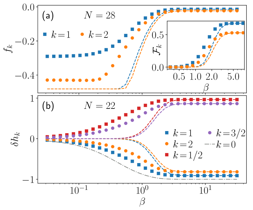
Figure 1: (a) Fidelity density and (b) deviation of staggered magnetization density as a function of temperature in the PXP model. Inset of (a) shows the fidelity. All quantities show strong deviation from the naive expectation of Eqs. (5) and (6) denoted by the dashed lines of the same color.

Classical simulation.—The dynamics of $\mathcal{F}_{k}$, $f_{k}$, and $h_{k}$ are obtained via exact diagonalization and plotted in Fig. 1 for various system sizes indicated in the legend. For reference, we also plot the predictions of Eqs. (5) and (6) with dashed lines. Surprisingly, Fig. 1 shows that, for all the metrics, there are strong deviations from theoretical predictions. An obvious reason for the mismatch between numerics and theoretical predictions could be finite-size effects. This appears unlikely, however, as a sensitive quantity such as the fidelity density is well converged in system size, as shown in Fig. 2 for an illustrative point $\beta\sim 1$, away from both the $\beta\approx 0$ and $\beta\to\infty$ regimes. One can clearly observe fidelity peaks at times that are multiples of $\tau\approx 4.8$, which coincides with the known revival period of the PXP model Turner et al. (2018b). Consequently, we still see strong deviations in $f_{k}$ and $\mathcal{F}_{k}$ at large system size $N=28$, where $\mathcal{D}=710647$, while for $h_{k}$ we probed system sizes up to $N=22$, where $\mathcal{D}=39603$. A detailed study of finite-size scaling of $f_{k}$ and $\delta h_{k}$ is provided in Fig. 2(b). These results show that both quantities are well converged already at $N\approx 20$, and we expect the observed behavior to persist in larger systems, including the larger-than-expected fidelity density near infinite temperature.

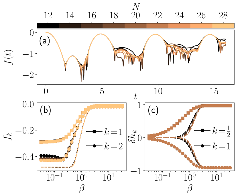
Figure 2: Fidelity density and observables after a quench in the PXP model. (a) Fidelity density over time for different system sizes for $\beta=0.89$, away from the high- and low-temperature regimes. (b) Fidelity density and (c) observable extrema. The dashed lines correspond to the theoretical expectations of Eqs. (5) and (6) for $k=1$. Both metrics are well converged in system size and show robustness to finite temperature when compared to the expected behavior.

Another possibility for the mismatch between numerics and theory in Fig. 1 could be due to unjustified assumptions in the latter. We test this in Fig. 3 where we compute the fidelity in the case where the ground state is artificially brought to infinite energy. We can engineer this by including an energy penalty $V\outerproduct{E_{0}}{E_{0}}$, with $V{\to}\infty$, in $\hat{H}_{i}$. Not only are clear revivals visible when the ground state is excluded, the same is true when the first set of excitations is excluded as well. This indicates that the presumption that only the ground states gives a significant contribution is not correct, accounting for the discrepancy with the theoretical predictions.

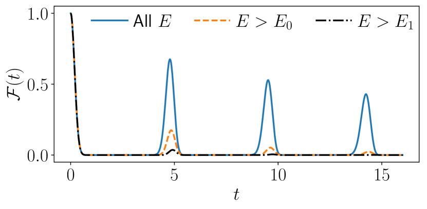
Figure 3: Interferometric amplitude after a quench in the pure PXP model for $N=28$ at zero temperature with energy penalties placed on the low-energy spectrum. Revivals can be seen even when the ground state and the first set of excited states are excluded from the initial Gibbs state.

Quantum simulation.—Our previous results for the PXP model strongly suggest that scarring signatures persist at finite temperature. We now demonstrate that this robustness can be witnessed in current experimental devices. We have employed the IBM quantum processor, Kolkata, which uses a heavy hex topology and has quantum volume $128$ IBM , to simulate finite-$T$ quenches in the PXP model. The IBM processors use a cross-resonance gate to generate the CNOT entangling operation. On this hardware, we simulated the time dependence of the staggered magnetization, $\hat{M}_{S}$, in Eq. (3). We simulate the evolution of the system under the Hamiltonian (2) but now, for convenience, assuming open boundary conditions. As in the classical simulations, we simulate evolution for an initial Gibbs state (1) at temperature $1/\beta$, working fully within the constrained Hilbert space. However, rather than preparing the thermal state (1) explicitly on the quantum computer, we use the $E\rho Oq$ method Gustafson and Lamm (2021); Lamm and Lawrence (2018); Harmalkar et al. (2020), which involves sampling from the density matrix (1) via the traditional Markov Chain Monte Carlo (MCMC) method, see SM SOM for details. In particular, to the authors’ best knowledge, this is the largest-scale demonstration of the $E\rho Oq$ algorithm on quantum hardware to date. We have used the suite of error mitigation techniques provided by QISKit Runtime Qiskit contributors (2023); run (2021), which include: dynamic decoupling Wrikat (2019); Ezzell et al. (2022); Qi et al. (2023); Morong et al. (2023); Jurcevic et al. (2021); Niu and Todri-Sanial (2022a, b); Mundada et al. (2023); Team (2022), randomized compiling Wallman and Emerson (2016a); Erhard et al. (2019); Li and Benjamin (2017); Endo et al. (2018); Geller and Zhou (2013); Wallman and Emerson (2016b); Silva et al. (2008); Winick et al. (2022), and readout mitigation (specifically T-REx) Pitsun et al. (2020); Mundada et al. (2019); Heinsoo et al. (2018); Sarovar et al. (2020); van den Berg et al. (2022); Smith et al. (2021); Rudinger et al. (2021); Tannu and Qureshi (2019); Harrigan et al. (2021); Chen et al. (2019); Maciejewski et al. (2020); Nachman et al. (2020); Hicks et al. (2022); Gong et al. (2019); Wei et al. (2020); Hamilton et al. (2020); Geller and Sun (2021); Song et al. (2017). We also used a rescaling procedure to counteract the signal loss from the effective depolarizing channel caused by the randomized compiling Urbanek et al. (2021); Vovrosh et al. (2021); A Rahman et al. (2022).

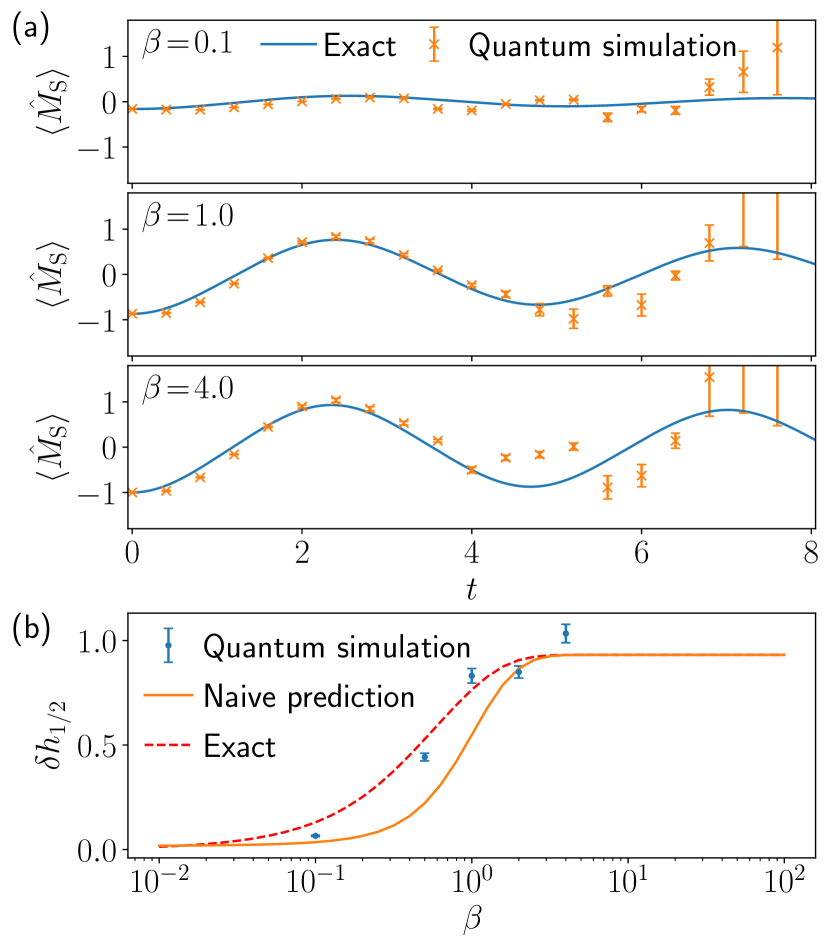
Figure 4: (a) Time dependence of $\hat{M}_{\mathrm{S}}$ for $\beta\in\{0.1,1,4\}$ in the PXP model with $8$ qubits and OBC. The experimental data shows good agreement with the numerical simulations. (b) Relative deviation after a half period of $\langle\hat{H}_{i}\rangle/N$ from its predicted value of Eq. (6). The quantum simulation data shows larger deviation than the naive expectation. In both panels, the error bars correspond to partial systematic errors from rescaling and statistical sampling from the density matrix. The simulations for $\beta=2$ were run on July 26, 2023 and all other $\beta$ on August 4th.

We have simulated the PXP model at $5$ different inverse temperatures $\beta\in\{0.1,0.5,1,2,4\}$ and generated $N_{c}=10^{5}$ configurations at each $\beta$. The time-evolution operator was decomposed using the Trotter approximation with a time step of $\delta t=0.4$. The time evolution of $\hat{M}_{\mathrm{S}}$ is shown for $8$ qubits in Fig. 4(a) for $\beta\in\{0.1,1,4\}$. While this is a relatively small system, the PXP model is known to be difficult to simulate even with advanced error-mitigation techniques Chen et al. (2022). We find that a reliable signal for the time dependence can be obtained up to one oscillation or roughly ten Trotter steps. From this data, we can extract $\delta h_{k}$; in fact, as $\langle\hat{h}_{i}\rangle_{\beta=0}=1$, it is straightforward to see that $\delta\hat{h}=\hat{M}_{\mathrm{S}}$. In Fig. 4(b), we plot $\delta h_{1/2}$ for our quantum simulation along with the exact results. Both show larger deviations from the thermal value that our naive expectation would predict in Eqs. (5) and (6). While we need to keep in mind the small system size used, which limits the accuracy of our prediction based solely on the ground-state contributing, its relatively good agreement with the exact data means that we can expect the same kind of behavior in larger systems.

Conclusions and discussion.— We have studied the fate of QMBS revivals at finite temperature in the PXP model. The initial density matrix at temperature $1/\beta$ is produced by an annealing procedure, instead of the usual pure states previously considered in the literature. We have observed robust QMBS signatures at finite temperature in both the fidelity and local observables. Finite-size scaling shows that this behavior is well converged within the accessible system sizes. Using a digital quantum computer, we have demonstrated persistent QMBS revivals in the IBM device at finite temperature.

In order to understand the origin of the observed robustness of scarring, we have studied in the SM SOM finite-$T$ quenches for the perturbed PXP model with nearly perfect scarring Khemani et al. (2019); Choi et al. (2019) as well as other models with analogous QMBS states, such as the spin-$1$ XY magnet Schecter and Iadecola (2019). While PXP perturbations yield essentially the same results as presented above, the behavior of the spin-$1$ XY model is found to be completely different: the low-$T$ behavior of the return fidelity as well as the oscillations of observables are now well described by Eqs. (5)-(6), implying that only the $T=0$ state gives a non-vanishing contribution and the QMBSs are much more fragile.

We attribute the difference in finite-$T$ behavior between the PXP and other models to the different algebraic properties of their QMBS states. Namely, the QMBS states in the PXP model form a representation of a large $\mathrm{su}(2)$ spin Choi et al. (2019), which is a special case of the “restricted spectrum generating algebra” that describes many other QMBS models, including the mentioned spin-$1$ XY magnet Moudgalya et al. (2022b); Mark et al. (2020); O’Dea et al. (2020). In most of these models, the non-thermal eigenstates are completely decoupled from the thermal bulk, hence they exactly form a single algebra representation. By contrast, in the PXP model the algebra is inexact, due to the small residual couplings to the thermal bulk. Furthermore, the non-thermal eigenstates form towers of multiple $\mathrm{su}(2)$ representations that originate from a collective spin-$1$ degree of freedom Omiya and Müller (2023). This means that when starting from a finite-temperature ensemble in the PXP model, we can have coherent contributions from states belonging to different $\mathrm{su}(2)$ representations, which effectively “shield” QMBSs from finite temperature.

Unfortunately, due to a lack of an exhaustive construction of multiple $\mathrm{su}(2)$ representations in the PXP model, their impact on finite-$T$ quench dynamics remains a conjecture at this stage. One interesting direction to pursue would be to construct toy models with a controllable number of embedded algebra representations and probe their finite-$T$ behavior. On the other hand, it is worth noting that there are also other frameworks for building QMBS models that extend beyond the simple Lie algebra scheme considered here, e.g.,  O’Dea et al. (2020); Pakrouski et al. (2020); Moudgalya and Motrunich (2022), and it would be interesting to understand if any of them display a similar robustness to finite temperature.

SI Low-temperature approximation

Here we derive the expected behavior of the interferometric Loschmidt echo and of the expectation value of a local observable $\hat{h}_{i}$ in a scarred system following a quench.

SI.1 Interferometric Loschmidt echo

Let us first focus on the interferometric Loschmidt echo, defined in the main text as

$$\mathcal{F}(t)=\big{\lvert}{\Tr}\big{\{}e^{-i\hat{H}_{f}t}\hat{\rho}\big{\}}\big{\rvert}^{2}.$$ (S1)

Let us denote by $\ket{E_{n}}$ the eigenstates of $\hat{H}_{i}$ with eigenenergies $E_{n}$. As was done in the main text, we will assume $E_{0}=0$. For a given value of the inverse temperature $\beta$ (with respect to $\hat{H}_{i}$), our initial mixed state will then be given by

$$\hat{\rho}=\frac{1}{Z}\sum_{E_{n}}e^{-\beta E_{n}}\outerproduct{E_{n}}{E_{n}},$$ (S2)

where $Z$ is the partition function defined as

$$Z=\sum_{E_{n}}e^{-\beta E_{n}}.$$ (S3)

Substituting the expression for the density matrix, Eq. (S1) becomes

$$\mathcal{F}_{\hat{\rho}}(t)=\frac{1}{Z^{2}}\bigg{\lvert}\sum_{E_{n}}e^{-\beta E_{n}}\langle E_{n}|e^{-i\hat{H}_{f}t}|E_{n}\rangle\bigg{\rvert}^{2}.$$ (S4)

At times that are multiples of the period, $t=k\tau$, we know that $\langle E_{0}|e^{-i\hat{H}_{f}t}|E_{0}\rangle=\sqrt{\mathcal{F}^{\infty}_{k}}$, where the $0$ subscript denotes infinite $\beta$ (or equivalently zero temperature). Let us discuss the other eigenstates $\ket{E_{n}}$ with $n\neq 0$. We assume them to be thermalizing with respect to $\hat{H}_{f}$ and so we should get $\langle E_{n}|e^{-i\hat{H}_{f}t}|E_{n}\rangle\approx e^{-ir_{n}}/\sqrt{\mathcal{D}}$ for $t$ long enough, with $e^{-ir_{n}}$ essentially a random phase. As they are essentially random with a very small individual contribution, we can forget about their weights and consider their equal superposition. While this is not very accurate for larger values of $\beta$ where their weights can strongly vary, in that regime the contribution of the ground state completely dominates around $t=k\tau$. As such, any inaccuracy in the contribution of the other eigenstates will be effectively negligible. On the other hand, for small $\beta$ the ground state no longer dominates but the prefactor of each eigenstate is close to equal. Thus, our approximation is justified and we can rewrite

$$\mathcal{F}_{\hat{\rho}}(k\tau) =\bigg{\lvert}\frac{\sqrt{\mathcal{F}^{\infty}_{k}}}{Z}+\left(1-\frac{1}{Z}\right)\sum_{n\neq 0}\langle E_{n}|e^{-iH_{f}k\tau}|E_{n}\rangle\bigg{\rvert}^{2}$$ (S5)

$$\approx\bigg{\lvert}\frac{\sqrt{\mathcal{F}^{\infty}_{k}}}{Z}+\left(1-\frac{1}{Z}\right){\rm Tr}\left[e^{-iH_{f}k\tau}\right]\bigg{\rvert}^{2}.$$

Taking the expectation value, the cross product vanishes as its expectation value is zero for a chaotic system. Meanwhile ${\rm Tr}\left[e^{-iH_{f}k\tau}\right]|^{2}$ is simply the spectral form factor (SFF) and its expectation value is $1/\mathcal{D}$ once the Heisenberg time has been reached. Hence, the expectation value of $\mathcal{F}_{\hat{\rho}}(k\tau)$ for a long enough $\tau$ is

$$\mathbf{E}\left[\mathcal{F}_{\hat{\rho}}(k\tau)\right]=\frac{\mathcal{F}^{\infty}_{k}}{Z^{2}}+\frac{\left(1-\frac{1}{Z}\right)^{2}}{\mathcal{D}}.$$ (S6)

Note that, as the SFF is not self-averaging, we expect to reach this quantity in the thermodynamic limit only after averaging over a number of realizations, denoted by the probabilistic expectation $\mathbf{E}$. However, this gives us an idea of the expected behavior.

We can identify two leading contributions that contribute at different temperature regimes. At very low temperature, the ground state will be the main contribution, while at very high temperature the largest term will come from the thermal states. We are mostly interested in the low temperature regime, where we can still expect to see traces of ergodicity breaking. In this regime $\beta\gg 1$, we should have $\mathcal{F}(k\tau)\approx\mathcal{F}^{\infty}_{k}/Z^{2}$.

SI.2 Observables

We now derive an expression for the expectation value of $\hat{h}_{i}$ if only the ground states of $\hat{H}_{i}$ shows perfect revival in $\hat{H}_{f}$ and all its other eigenstates thermalize rapidly. As in the previous section, we denote by $\ket{E_{n}}$ the eigenstates of the pre-quench Hamiltonian $\hat{H}_{i}$ and by $\tau$ the revival period. The previous assumption then translates into the statement

$$\braket{E_{n}}{e^{-i\hat{H}_{f}\tau}}{E_{m}}=\delta_{0,0}+\frac{(1-\delta_{n,0})(1-\delta_{m,0})}{\sqrt{\mathcal{D}-1}},$$ (S7)

with $\mathcal{D}$ the Hilbert space dimension and $\tau$ is assumed to be large. This will prove useful to compute the expectation value of $\hat{h}_{i}=\frac{1}{N}\hat{H}_{i}$ over time, defined as

$$\braket{\hat{h}_{i}}(t)=\Tr{\hat{\rho}(t)\hat{h}_{i}}$$ (S8)

$$=\frac{1}{N}\sum_{n,m}P(E_{m})\bra{E_{n}}e^{-i\hat{H}_{f}t}\ket{E_{m}}\bra{E_{m}}e^{i\hat{H}_{f}t}\hat{H}_{i}\ket{E_{n}}$$

$$=\frac{1}{N}\sum_{n,m}P(E_{m})E_{n}\bra{E_{n}}e^{-i\hat{H}_{f}t}\ket{E_{m}}\bra{E_{m}}e^{i\hat{H}_{f}t}\ket{E_{n}}$$

$$=\frac{1}{N}\sum_{n,m}P(E_{m})E_{n}\big{\lvert}\bra{E_{n}}e^{-i\hat{H}_{f}t}\ket{E_{m}}\big{\rvert}^{2}$$

$$=\frac{1}{N}\sum_{n,m}P(E_{m})\tilde{E}_{n}\big{\lvert}\bra{E_{n}}e^{-i\hat{H}_{f}t}\ket{E_{m}}\big{\rvert}^{2},$$

with $P(E_{n})=e^{-\beta E_{n}}/Z$ and $\tilde{E}_{n}=E_{n}/N$. For $t=k\tau$ we can use the assumption made in Eq. (S7) to get

$$\braket{\hat{h}_{i}}(k\tau) \approx P(E_{0})\tilde{E}_{0}+\sum_{n\neq 0}\sum_{m\neq 0}\frac{P(E_{n})\tilde{E}_{m}}{\mathcal{D}-1}$$ (S9)

$$=P(E_{0})\tilde{E}_{0}{+}\left(\sum_{m\neq 0}P(E_{m})\right)\left(\frac{\sum_{n\neq 0}\tilde{E}_{n}}{\mathcal{D}-1}\right)$$

$$=P(E_{0})\tilde{E}_{0}{+}\left(1{-}P(E_{0})\right)\left(\frac{-\tilde{E}_{0}+\sum_{n}\tilde{E}_{n}}{\mathcal{D}{-}1}\right)$$

$$=P(E_{0})\tilde{E}_{0}{+}\left(1{-}P(E_{0})\right)\left(\frac{\mathcal{D}\braket{\hat{h}_{i}}_{\beta=0}{-}\tilde{E}_{0}}{\mathcal{D}{-}1}\right)$$

$$=P(E_{0})\tilde{E}_{0}{+}\left(1{-}P(E_{0})\right)\left(\frac{\mathcal{D}\braket{\hat{h}_{i}}_{\beta=0}{-}\tilde{E}_{0}}{\mathcal{D}{-}1}\right).$$

In the limit of large system sizes, we can take $\frac{\mathcal{D}}{\mathcal{D}-1}\to 1$ and $\frac{\tilde{E}_{0}}{\mathcal{D}-1}\to 0$, since $\tilde{E}_{0}=E_{0}/N$ is $\mathcal{O}(1)$. This leads to

$$\braket{\hat{h}_{i}}(\tau) =P(E_{0})\tilde{E}_{0}+\left(1-P(E_{0})\right)\braket{\hat{h}_{i}}_{\beta=0}$$ (S10)

$$=\braket{\hat{h}_{i}}_{\beta=0}+P(E_{0})\left(\tilde{E}_{0}-\braket{\hat{h}_{i}}_{\beta=0}\right)$$

$$=\braket{\hat{h}_{i}}_{\beta=0}+\frac{1}{Z}\left(\tilde{E}_{0}-\braket{\hat{h}_{i}}_{\beta=0}\right).$$

For a large enough system size, we expect both $E_{0}$ and $\braket{\hat{h}_{i}}_{\beta=0}$ to converge towards a finite value, and so in the infinite temperature limit where $Z=\mathcal{D}$ we recover $\braket{\hat{h}_{i}}_{\beta=0}$. On the other hand, at zero temperature we have that $Z=1$ and and we simply get $\tilde{E}_{0}=\braket{\hat{h}_{i}}_{\beta=\infty}$.

If we are now interested in the deviation from the infinite temperature value, we find the simple expression

$$\braket{\delta\hat{h}_{i}}(k\tau)=\frac{1}{Z}\left(\frac{\tilde{E}_{0}}{\braket{\hat{h}_{i}}_{\beta=0}}-1\right).$$ (S11)

In the simple case we consider here, we also have that $E_{0}=0$, leading to the even simpler formula of

$$\braket{\delta\hat{h}_{i}}(k\tau)=-\frac{1}{Z}.$$ (S12)

If the revivals are not perfect, after one revival the ground state wavefunction does not lead to a value of $\tilde{E}_{0}=0$ but instead to $h_{k}^{\infty}$. In that case we can simply replace $\tilde{E}_{0}$ by the this value to get

$$\braket{\delta\hat{h}_{i}}(k\tau)=\frac{1}{Z}\left(\frac{h_{k}^{\infty}}{\braket{\hat{h}_{i}}_{\beta=0}}-1\right).$$ (S13)

SII spin-$1$ XY model

In this section, we show results for finite-temperature quenches in the 1D spin-$1$ XY magnet Schecter and Iadecola (2019), where quantum many-body scar (QMBS) eigenstates can be exactly constructed. The spin-1 XY model is described by the Hamiltonian

$$\hat{H}_{f,\text{XY}} =\!J\sum_{j=1}^{N-1}\left(\hat{S}^{x}_{j}\hat{S}^{x}_{j+1}+\hat{S}^{y}_{j}\hat{S}^{y}_{j+1}\right)$$

$$+h\sum_{j=1}^{N}\hat{S}^{z}_{j}+D\sum_{j=1}^{N}\left(\hat{S}^{z}_{i}\right)^{2}$$

$$+J_{3}\sum_{j=1}^{N-3}\left(\hat{S}^{x}_{j}\hat{S}^{x}_{j+3}+\hat{S}^{y}_{j}\hat{S}^{y}_{j+3}\right).$$ (S14)

Unless specified otherwise, we will set $J=1$, $h=1$, $D=0.1$, and $J_{3}=0.1$ and assume open boundary conditions (OBCs). For these values of parameters, the model was shown to be non-integrable and displaying chaotic level statistics Schecter and Iadecola (2019). At the same time, preparing the system in the initial state

$$\ket{\psi_{0}}=\bigotimes_{j=1}^{N}\left[\frac{\ket{+1}-(-1)^{j}\ket{-1}}{\sqrt{2}}\right]$$ (S15)

was shown to give rise to perfect oscillatory dynamics Schecter and Iadecola (2019), revealing the existence of QMBSs. These oscillations can be understood as spin precession, due to the state $\ket{\psi_{0}}$ in Eq. (S15) having overlap on only $N+1$ scarred eigenstates of $\hat{H}_{f,\text{XY}}$. This motivates our choice of this model, as it admits a similar algebraic description as the PXP model, but with the added possibility of writing down the scarred eigenstates in closed analytic form.

Note that the state $\ket{\psi_{0}}$ has an expectation value of energy equal to $DN$, while the middle of the spectrum of $\hat{H}_{f}$ is at energy $2DN/3$. As we use a small value of $D$, the initial state is thus very close to infinite temperature with respect to $\hat{H}_{f}$ (e.g., for $N=8$ we find $\beta_{f}=8.8\times 10^{-3}$). In the remainder of this section, we repeat the computations of the same metrics as for the PXP model in the main text and contrast the behavior of the two models.

To prepare the state in Eq. (S15), we can use the pre-quench Hamiltonian proposed in Ref. Schecter and Iadecola (2019):

$$H_{i,\text{XY}}=\frac{N}{2}+\sum_{j=1}^{N}(-1)^{j}\left[\left(\hat{S}_{j}^{x}\right)^{2}-\left(\hat{S}_{j}^{y}\right)^{2}\right].$$ (S16)

The resulting thermal state at temperature $\beta$ will always be close to infinite temperature with respect to $\hat{H}_{f}$, warranting our expectation of thermalization to the corresponding ensemble.

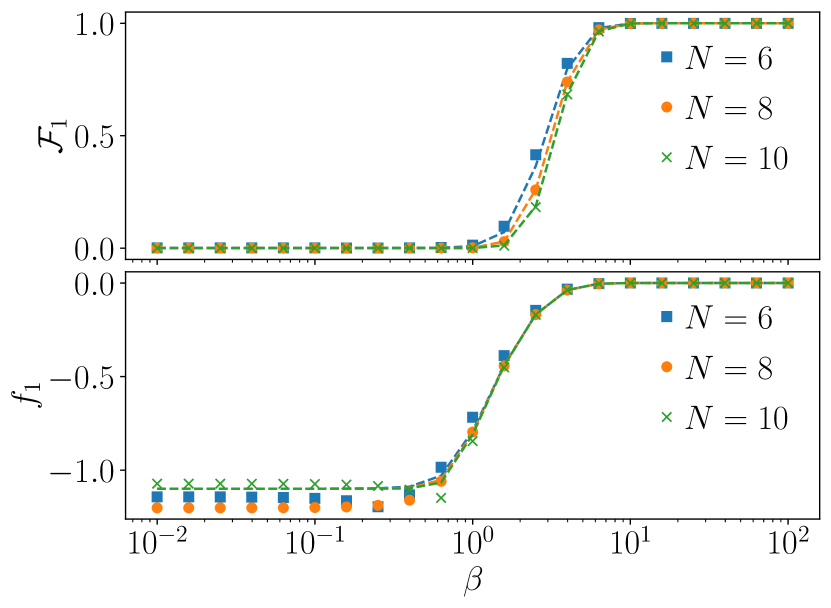
Figure S1: Maximum interferometric amplitude after a quench in the XY spin-$1$ model for various values of the temperature using the preparation Hamiltonian in Eq. (S16). The dashed lines show the expected scaling following Eq. (5), with the partition function given by Eq. (S17). The agreement with the expect scaling should be contrasted with the PXP model in Fig. 1.

Figure S1 shows $\mathcal{F}_{1}$ after a quench along with its theoretical counterpart, computed using

$$Z=(1+e^{-\beta}+e^{-2\beta})^{N},$$ (S17)

which is straightforward to obtain as the Hamiltonian $\hat{H}_{i,\text{XY}}$ is non-interacting. The agreement with the prediction is quite good, showing that the contribution to revivals of states above the ground state is indeed very small.

To further verify how much these states impact the dynamics, we investigate the scenario where an energy penalty $V\outerproduct{E_{0}}{E_{0}}$ with $V\to\infty$ is added to the preparation Hamiltonian. This essentially removes the ground state while leaving the rest of the spectrum completely untouched due to the orthogonality of eigenstates. We plot results for this and for the case where the first set of excited states are also removed in Fig. S2.

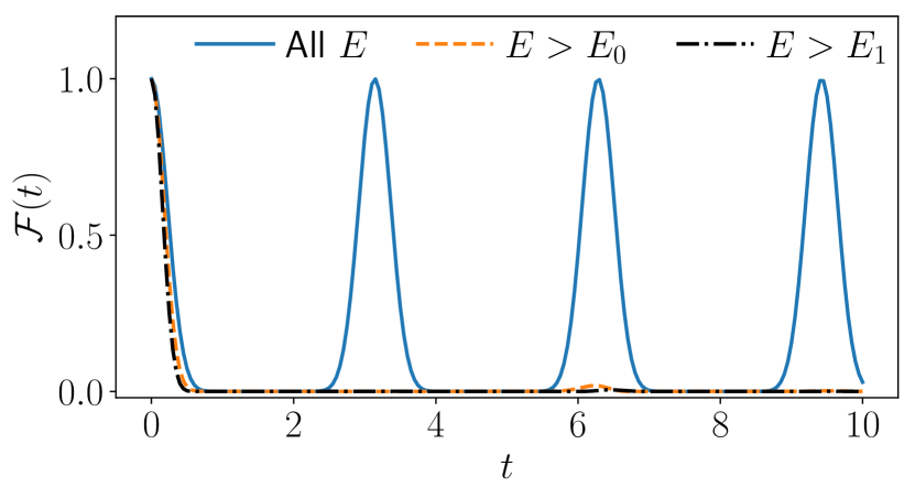
Figure S2: Maximum interferometric amplitude at zero temperature after a quench in the XY spin-$1$ model with $N=10$ and using $\hat{H}_{i}$ in Eq. (S16). Various energy penalties on the low-energy spectrum are compared. The perfect revivals in the top panel and their absence in the bottom two panels should be contrasted with the PXP case in Fig. 3.

We see that the revivals are destroyed, except from small fluctuations that are expected to decay with system size.

Finally, we study the deviation of the expectation value of $\hat{H}_{i}/N$ to the thermal value after a quench, as shown in Fig. S3. Overall, we see that our approximation of any non-thermalizing dynamics stemming solely from the ground state holds well.

Figure S3: Extremal value of $\langle\hat{h}_{i}\rangle$ around $t=k\tau$ for the spin-$1$ XY model with system size $N=9$ and using $\hat{H}_{i}$ in Eq. (S16). The dashed black line indicates the theoretical prediction from Eq. (6). It provides a good approximation to the exact dynamics, despite the much smaller system size and Hilbert space size in this case compared to the PXP model in Fig. 1.

SIII Alternative preparation Hamiltonian for the XY model

In order to compare more directly our results of the XY model with those of PXP model, here we use an alternative preparation Hamiltonian than holds a closer relation with the algebraic structure of the scarred states. This will have the effect of enhancing the overlap of states in the low-energy spectrum with scarred eigenstates. We now use the pre-quench Hamiltonian

$$\hat{H}^{(2)}_{i,\text{XY}}=\!\sum_{j=1}^{N}(-1)^{j}\left[\left(\hat{S}_{j}^{x}\right)^{2}{-}\left(\hat{S}_{j}^{y}\right)^{2}\right]\!{+}V\!\prod_{j=1}^{N}\left[\hat{\mathds{1}}_{j}{-}\left(\hat{S}_{j}^{z}\right)^{2}\right].$$ (S18)

Note that with respect to the preparation Hamiltonian in Eq. (S16), the additional term $\propto V$ has been added. This has no effect on the ground state. However, if we choose $V\gg 1$ this heavily penalizes any occurrence of the $\ket{0}$ state. As a consequence, the first excited states have a single $(\ket{+1}\pm\ket{-1})/\sqrt{2}$ turned into $(\ket{+1}\mp\ket{-1})/\sqrt{2}$. The additional excitation will follow the same scheme, and the states with $\ket{0}$ sites — which are orthogonal to scarred states — will only contribute at large temperature. Effectively, this Hamiltonian acts as the $\hat{J}^{x}$ operator of the effective $\mathrm{su}(2)$ algebra, while $\hat{H}_{f}$ acts as $\hat{J}^{z}$ in the scarred subspace. The same relation is obeyed with $\hat{H}_{i}$ and $\hat{H}_{f}$ in the PXP model.

One of the main effects of this is that the symmetric superposition of the first set of excited states is entirely contained in the scarred subspace. So we now get that one state in the $N$ first excited states is meaningful for revivals. This is similar to the situation in the PXP model, where one state out of the $N/2$ in the first set of excitations belongs to the scarred subspace. However, this contribution still goes to 0 as $N\to\infty$. In the rest of this section, we set $V=50$. In order to adapt our analytic expectation to this change, we change $Z$ to

$$Z= \,(1{+}e^{{-}2\beta})^{N}$$

$${+}e^{{-}\beta V}\left[(1{+}e^{{-}\beta}{+}e^{-2\beta})^{N}{-}(1{+}e^{{-}2\beta})^{N}\right],$$ (S19)

which is very close to simply $(1{+}e^{{-}2\beta})^{N}$ for $\beta>10^{-1}$. Indeed, while away from the $\beta\ll 1$ regime, the initial state has essentially no overlap with any state with a $\ket{0}$ site. Results for this case are shown in Fig. S4.

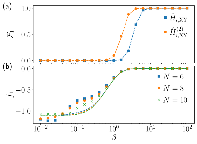
Figure S4: Maximum interferometric amplitude after a quench in the XY spin-$1$ model for various values of the temperature. The dashed lines indicate the expected scaling for the data of the same color. (a) Comparison between the preparation Hamiltonians in Eqs. (S16) and (S18) for $N=10$. (b) Quenches using the preparation Hamiltonian in Eq. (S18) for various system sizes. While there are some deviations from the expected behavior, they decay with system size and only happen for very low values of the fidelity density.

While we see a good fidelity compared to the original pre-quench Hamiltonian in Eq. (S16), this is essentially due to the difference of the weight on the ground state as captured by the analytic prediction. There are also some small deviations with respect to the theoretical prediction for $\beta\approx 0.1$, but they clearly decay with system size. They also happen in a regime where the observed fidelity is effectively zero, meaning that traces of scarring in the system will be extremely difficult to measure. This showcases that, as seen with the previous preparation Hamiltonian, only the ground state of $\hat{H}_{i}$ is expected to contribute to the non-ergodic dynamics in the thermodynamic limit.

This is confirmed by quenches where the contribution of the ground state is artificially removed by setting an energy penalty on it; see Fig. S5. While the peak in the middle panel is slightly larger than in Fig. S2, the difference is small and expected to decay with system size.

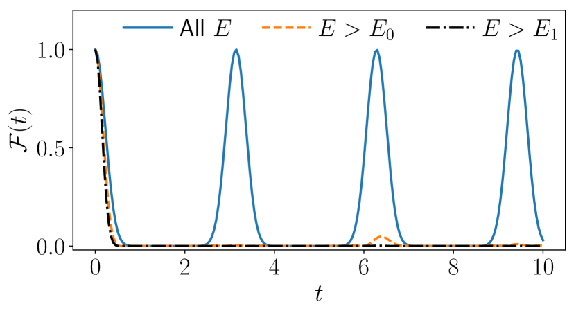
Figure S5: Interferometric amplitude after a quench in the XY spin-$1$ model with $N=10$ using the preparation Hamiltonian in Eq. (S18). Various energy penalties on the low-energy spectrum are compared. The only visible difference with Fig. S2 is the slightly larger amplitude of the fluctuations around $t=2\tau$.

SIV Perturbed PXP model

While the QMBS phenomenology in the spin-$1$ XY model resemble that of the PXP model discussed in the main text, one obvious difference is that the former hosts exact QMBS and perfect revivals. Thus, in order to be able to compare the two models on the same footing, we consider the perturbed version of the PXP model, $\hat{H}_{f}^{\mathrm{PXP}}+\delta\hat{H}$, in which scarring is essentially perfect. This perturbation was devised in Ref. Choi et al. (2019) and takes the form

$$\delta\hat{H}=\;-\sum_{j=1}^{N}\sum_{d=2}^{N/2}h_{d}\hat{P}_{j-1}\hat{\sigma}^{x}_{j}\hat{P}_{j+1}\left(\hat{\sigma}^{z}_{j-d}+\hat{\sigma}^{z}_{j+d}\right),$$ (S20)

with

$$h_{d}=h_{0}\left(\phi^{d-1}-\phi^{1-d}\right)^{-2},$$ (S21)

$h_{0}=0.051$, and $\phi=(1+\sqrt{5})/2$ the golden ratio. The first order term in this expansion was also considered in Ref. Khemani et al. (2019). Low-order terms of an expansion such as Eq. (S20) can be iteratively derived in a process of “correcting” the structure constants of the $\mathrm{su}(2)$ algebra representation, furnished by QMBS eigenstates Bull et al. (2020). Thus, the perturbation in Eq. (S20) makes the revivals from the Néel state essentially perfect and the associated algebra in the QMBS subspace nearly $\mathrm{su}(2)$, allowing for a much closer comparison with the spin-$1$ XY model.

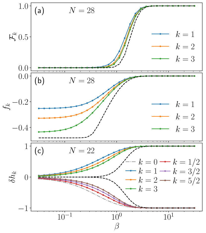
Figure S6: Fidelity, fidelity density, and deviation of observable density for various values of the temperature in the perturbed PXP model. All quantities show strong deviation from the naive expectation denoted by the dashed black lines.

Using the perturbed PXP model in Eq. (S20), we repeat the computations for the pure PXP model given in the main text, in order to check to what extent the exactness of QMBS structure impacts the conclusions. The dynamics of $\mathcal{F}_{k}$, $f_{k}$, and $h_{k}$ for the perturbed PXP model are shown in Fig. S6. For all metrics, we see strong deviations from the naive thermal predictions. In Fig. S7 we compute the fidelity in the case where the ground state is artificially brought to infinite energy. Not only are clear revivals visible when the ground state is excluded, the same is true when the first set of excitations is excluded as well. The symmetric superposition of all states with one defect on top of the Néel state should have overlap exclusively on scarred eigenstates. However, the other $N/2-1$ superpositions will be orthogonal to it, and should theoretically not contribute to the revivals. Thus, as only one state out of $N/2$ contribute, we expect its contribution to be similar to what was seen in the XY model. The next set of excitations is then made of the Néel state with two defects. As once again only the symmetric superposition is in the scarred subspace, this concerns one state in $N(N/2-1)/2$. Overall, one would expect the behavior to be the same as in the XY model, but it clearly is not.

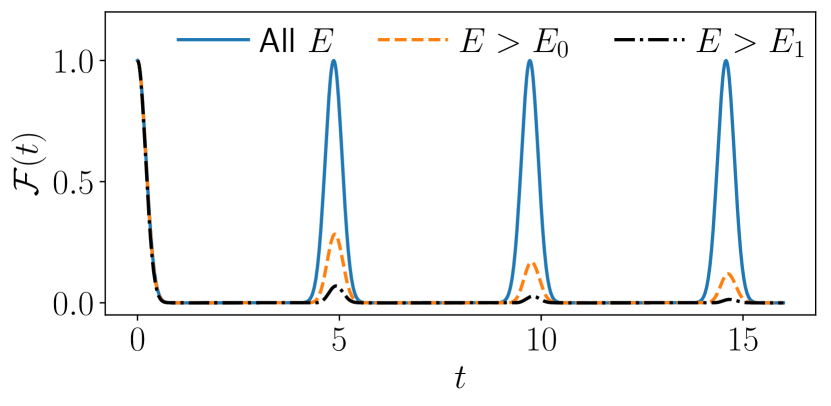
Figure S7: Interferometric amplitude after a quench in the perturbed PXP model for $N=28$ with energy penalties placed on the low-energy spectrum. Clear revivals can be seen even when the ground state and the first set of excited states are removed.

We emphasize that what we witness in the PXP model is not a finite-size effect. Actually, the Hilbert space sizes explored in this model are larger than the ones in the XY model. Indeed, in the latter we saw good agreement with the theoretical predictions already for $N=8$ and $N=10$, corresponding to $\mathcal{D}=3^{9}=19683$ and $\mathcal{D}=3^{10}=59049$, respectively. Meanwhile, in the PXP model we still see strong deviations in $f_{k}$ and $\mathcal{F}_{k}$ for $N=28$ where $\mathcal{D}=710647$, an order of magnitude larger. For $h_{k}$ we probed system sizes up to $N=22$ where $\mathcal{D}=39603$. Furthermore, we provide the scaling of $f_{k}$ and $\delta h_{k}$ with system size in Fig. S8. Our results show that both quantities are well converged already at $N\approx 20$. As such, we expect the same special behavior in larger systems. This includes the higher-than-expected fidelity density near infinite temperature.

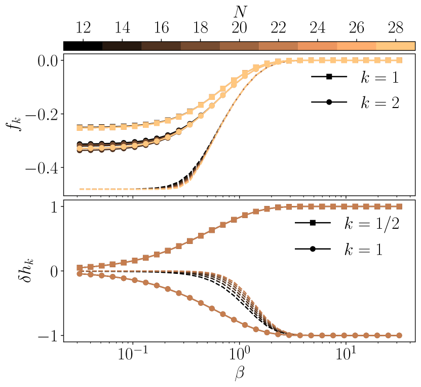
Figure S8: Scaling of fidelity density and deviation of $\hat{H}_{i}/N$ after a quench in the perturbed PXP model. The dashed lines correspond to the theoretical expectations. Both metrics are well converged in system size and show robustness to finite temperature when compared to the expected behavior.

SV Details of the quantum algorithm

To simulate the PXP model, we have employed the IBM quantum processor, Kolkata, which uses a heavy hex topology and has quantum volume $128$ IBM . The IBM processors use a cross-resonance gate to generate the CNOT entangling operation. On this hardware, we simulated the time dependence of the staggered magnetization, $\hat{M}_{S}$ in Eq. (3). We simulate the evolution of the system under the Hamiltonian in Eq. (2) but now, for convenience, assuming open boundary conditions. The boundary terms in the Hamiltonian are taken to be $\hat{\sigma}^{x}_{1}\hat{P}_{2}$ and $\hat{P}_{N-1}\hat{\sigma}^{x}_{N}$.

As in all the classical simulations in this work, our goal is to simulate evolution for an initial Gibbs state at temperature $\beta$, as defined in Eq. (1). This must be done in the constrained Hilbert space where there are no neighboring $\ket{\uparrow}$, thus we only consider states in this subspace for our initial state. The time dependence of $\hat{M}_{S}$ can be explicitly written as

$$\langle\hat{M}_{\mathrm{S}}(t)\rangle{=}\sum_{E_{k}}\frac{e^{-\beta E_{k}}}{Z}\langle E_{k}|\hat{U}^{\dagger}(t)\hat{M}_{\mathrm{S}}\hat{U}(t)|E_{k}\rangle,$$ (S22)

where we recall that the $\ket{E_{k}}$ are the eigenstates of $\hat{H}_{i}$ in the constrained Hilbert space. At this point, we can see that it is sufficient to perform a simulation for all the states in $\hat{\rho}$, and perform a weighted average using their Boltzmann weights, $e^{-\beta E_{k}}/Z$.

We prepare the thermal state from Eq. (1) using the $E\rho Oq$ method Gustafson and Lamm (2021); Lamm and Lawrence (2018); Harmalkar et al. (2020). this method involves sampling states from the density matrix in Eq. (1) using traditional Markov Chain Monte Carlo (MCM) methods rather than preparing the thermal state explicitly on the quantum computer.

We generate configurations from the Hamiltonian in Eq. (3) as follows. Because the Hamiltonian in Eq. (3) is diagonal, the density matrix can be written as a diagonal operator

$$\hat{\rho}_{i}(\beta)=\frac{1}{Z}\sum_{\{\mathcal{S}_{j}\}}e^{-\beta E_{\mathcal{S}_{j}}}|\mathcal{S}_{j}\rangle\langle\mathcal{S}_{j}|,$$ (S23)

where the sum over $\{\mathcal{S}_{j}\}$ includes only the allowed spin configurations. We can now identify a corresponding action $S=\hat{H}_{i}$. The system is prepared in a valid spin configuration and spin changes are proposed randomly in MCMC sweeps with a given probability weighted by the change in total energy: $e^{-\beta(E_{\mathcal{S}^{\prime}}-E_{\mathcal{S}})}$. If a proposed change would take the system to an invalid subspace the proposed change is discarded. After generating $N_{c}$ configurations of the form $|\mathcal{S}_{j}\rangle\langle\mathcal{S}_{j}|$ from the density matrix, we then simulate the time dependence of $\hat{M}_{S}$ for each unique spin configuration. The thermal average is then the weighted average,

$$\langle\hat{M}_{\mathrm{S}}(t)\rangle=\sum_{\{\mathcal{S}_{i}\}}\frac{p_{i}}{N_{c}}\langle\mathcal{S}_{i}|\hat{U}^{\dagger}(t)\hat{M}_{\mathrm{S}}\hat{U}(t)|\mathcal{S}_{i}\rangle,$$ (S24)

where $p_{i}$ is the number of times the configuration appeared in the simulation. If an nondiagonal Hamiltonian is used for state preparation then linear combinations of the bra and ket vectors in the density matrix need to be used. In principle the accuracy of this method encounters an exponential signal to noise problem that is slightly lessened by the use of a diagonal Hamiltonian Harmalkar et al. (2020); Lamm et al. (2020).

We used the suite of error mitigation techniques provided by QISKit Runtime Qiskit contributors (2023); run (2021), which include: dynamic decoupling Wrikat (2019); Ezzell et al. (2022); Qi et al. (2023); Morong et al. (2023); Jurcevic et al. (2021); Niu and Todri-Sanial (2022a, b); Mundada et al. (2023); Team (2022), randomized compiling Wallman and Emerson (2016a); Erhard et al. (2019); Li and Benjamin (2017); Endo et al. (2018); Geller and Zhou (2013); Wallman and Emerson (2016b); Silva et al. (2008); Winick et al. (2022), and readout mitigation (specifically T-REx) Pitsun et al. (2020); Mundada et al. (2019); Heinsoo et al. (2018); Sarovar et al. (2020); van den Berg et al. (2022); Smith et al. (2021); Rudinger et al. (2021); Tannu and Qureshi (2019); Harrigan et al. (2021); Chen et al. (2019); Maciejewski et al. (2020); Nachman et al. (2020); Hicks et al. (2022); Gong et al. (2019); Wei et al. (2020); Hamilton et al. (2020); Geller and Sun (2021); Song et al. (2017). Dynamic decoupling is a method which aims to tackle dephasing errors that a quantum state accumulates by frequent applications of quantum gates on idling qubits which act to cancel accumulated phase errors. Randomized compiling is used to transform the unitary errors from the CNOT gate being imperfect into random stochastic Pauli errors which are typically less catastrophic. Readout mitigation is a tool which takes the output probability distribution measured from the quantum computer and changes the relative bitstring outputs using apriori knowledge determined when the quantum computer is calibrated on the likelihood of misidentify a $|0\rangle$ or $|1\rangle$ state. We also used a rescaling procedure to counteract the signal loss from the effective depolarizing channel caused by the randomized compiling Urbanek et al. (2021); Vovrosh et al. (2021); A Rahman et al. (2022). This method works by running a circuit which contains only Clifford gates and has a known classical output and using the discrepancy between the measured and expected value to renormalize the observed value.