Light Field Diffusion for Single-View Novel View Synthesis

Abstract

Single-view novel view synthesis, the task of generating images from new viewpoints based on a single reference image, is an important but challenging task in computer vision. Recently, Denoising Diffusion Probabilistic Model (DDPM) has become popular in this area due to its strong ability to generate high-fidelity images. However, current diffusion-based methods directly rely on camera pose matrices as viewing conditions, globally and implicitly introducing 3D constraints. These methods may suffer from inconsistency among generated images from different perspectives, especially in regions with intricate textures and structures. In this work, we present Light Field Diffusion (LFD), a conditional diffusion-based model for single-view novel view synthesis. Unlike previous methods that employ camera pose matrices, LFD transforms the camera view information into light field encoding and combines it with the reference image. This design introduces local pixel-wise constraints within the diffusion models, thereby encouraging better multi-view consistency. Experiments on several datasets show that our LFD can efficiently generate high-fidelity images and maintain better 3D consistency even in intricate regions. Our method can generate images with higher quality than NeRF-based models, and we obtain sample quality similar to other diffusion-based models but with only one-third of the model size.

1 Introduction

Novel view synthesis, the inference of a 3D scene’s appearance from novel viewpoints given several images of the scene [53, 29, 30, 49, 8, 58], plays a fundamental role in many computer vision applications such as game studios, virtual reality, and augmented reality [25, 5, 48]. This task requires that synthesized images not only match specific novel viewpoints but also ensure the shape and details are consistent with the reference images, i.e., multi-view consistency.

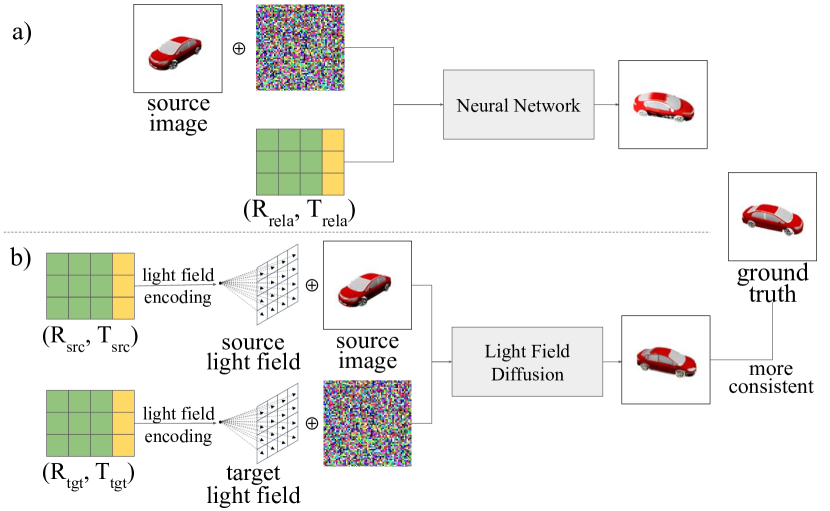
Figure 1: Comparison of our Light Field Diffusion and previous diffusion-based models for single-view novel view synthesis: a) Previous models [53, 21] directly take camera pose matrices (rotation R and translation T) as input, which can only provide 3D constraints globally and implicitly. b) Our Light Field Diffusion transforms the camera pose matrices into light field encoding and concatenates them with the noise and source image, which provides local and explicit pixel-wise 3D geometry constraints, enabling better multi-view consistency.

Recently, Neural Radiance Fields (NeRF) [23] has made significant advancements in the area of novel view synthesis. NeRF represents a scene using a multi-layer perception (MLP) and uses volume rendering to generate an image, enabling realistic 3D renderings and multi-view consistency. In spite of its great success, the training process of NeRF typically requires dense views from different angles and corresponding camera poses, posing a challenge for its practical application in real-world scenarios. To this end, later works focus on learning a NeRF in the sparse view settings [57, 27], which either utilize prior knowledge from pre-trained models on large-scale datasets [57, 20] or introduce regularization on geometry [27]. Moreover, some recent works [55, 20] try to train NeRFs to generate new images from different views with only one reference image, i.e., single-view novel view synthesis. This task is exceptionally demanding for regression-based methods like NeRF [53]. Without sufficient information from other views, NeRF suffers from incorrect learning in 3D geometry, which often results in blurred outputs [27].

On the other hand, generative methods, especially Diffusion Probabilistic Model (DDPM) [13, 43, 41], have become popular in the field of novel view synthesis [21, 2, 56, 53, 60, 33] due to their strong ability in single-view novel view synthesis with large view rotations. Of these approaches, one line of research combines the merits of NeRF with diffusion models [56, 11] and shows that these two types of methods can guide and boost each other. Other approaches directly train a conditional diffusion model in an end-to-end manner. Notably, 3DiM [53] is a pioneering work that learns a diffusion model conditioned on camera pose matrices of both views. In subsequent developments, Zero-1-to-3 [21] accomplishes this by refining the pre-trained stable diffusion model [32] using relative camera rotation and translation as conditions. This approach leverages the ample 3D priors inherent in large-scale diffusion models, despite being trained primarily on 2D images.

Although these end-to-end methods achieve great performance, they usually ignore the fact that the camera pose matrices can only provide 3D constraints globally and implicitly. As a result, these methods usually require a heavy network with billions of parameters to learn the implicit 3D constraint. Moreover, the generated images in different views may suffer pixel-wise inconsistency with the reference image. Therefore, it is imperative to establish an effective camera pose representation within these end-to-end diffusion-based methods for novel view synthesis.

To address the above issue, we propose Light Field Diffusion (LFD), a novel framework for single-view novel view synthesis based on DDPM [13]. Instead of relying directly on camera pose matrices, LFD takes a different approach by converting these matrices into pixel-wise camera pose encodings based on light field [19, 39], which includes the ray direction of each pixel and the camera origin. In detail, we concatenate this light field encoding with both the target image and reference image to involve camera pose information, and we use cross-attention layers to model the relationship between reference and target. This design facilitates the establishment of local pixel correspondences between the reference and target images, ultimately enhancing multi-view consistency in the generated images. Figure 1 summarizes an overall comparison between our method and previous end-to-end diffusion-based models in novel view synthesis.

We summarize our contributions as follows:

• We present a novel framework called Light Field Diffusion, which is an end-to-end conditional diffusion model designed for synthesizing novel views using just a single reference image. Instead of directly employing camera pose matrices, we employ a transformation into pixel-wise light field encoding. This approach harnesses the advantages of local pixel-wise constraints, resulting in a significant enhancement in model performance.

• Our method is demonstrated to effectively synthesize novel views that maintain consistency with the reference image, ensuring viewpoint coherence and producing high-quality results on both the ShapeNet Car [3] and Neural 3D Mesh Renderer [17] datasets.

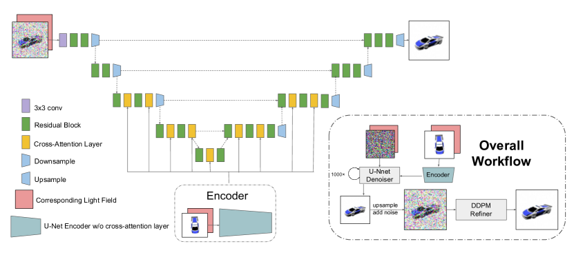
Figure 2: Architecture of Light Field Diffusion. Light Field Diffusion contains two parts: the U-Net Denoiser and the super-resolution module. We modify the U-Net Denoiser in DDPM by replacing the self-attention layer with the cross-attention layer. A separate encoder is used to extract features from the source image and source light field encoding. We use cross-attention layers to combine the extracted features and target light field encoding. The separate encoder has the same structure as the U-Net Denoiser Encoder but without cross-attention layers. Light Field Diffusion is trained to predict the original target image given the noisy target image, target light field encoding, and features from the encoder. All images are downsampled to $64\times 64$ during training. In the inference stage, we use a super-resolution module to upsample and optimize the results from U-Net Denoiser.

2 Related Work

2.1 NeRF in Novel View Synthesis

Neural Radiance Fields (NeRFs) [23, 57, 27, 20, 55, 14, 15, 38] have exhibited promising results in the realm of novel view synthesis. In detail, NeRFs employ a fully connected neural network to establish a mapping from viewing direction and spatial location to RGB color and volume density, enabling the rendering of views by projecting rays into 3D space and querying the radiance field at various points along each ray for each pixel on the image plane. Consequently, NeRF can guarantee 3D consistency among generated images. However, the vanilla NeRF is a scene-specific model, and it usually requires a dense view sampling of the scene, which may be impractical for complicated scenes. Since then, there have been multiple following works that improve the quality and generalization ability of NeRFs [57, 14, 27, 20, 4, 50, 55].

For instance, PixelNeRF [57] uses a CNN feature extractor pre-trained on large-scale datasets to extract context information features and conduct NeRF in feature map space. VisionNeRF [20] integrates both global features from a pre-trained ViT [7] model and local features from pre-trained CNN encoders. DietNeRF [14] supervises the training process by a semantic consistency loss using the CLIP encoder [31]. Most recently, researchers have pushed NeRF to single-view novel view synthesis [57, 55]. SinNeRF [55] resorts to the depth map of the single reference image and proposes a semi-supervised framework to guide the training process of NeRF. However, due to the properties of regressive models, all these NeRF-based approaches suffer from blurred results when the view rotation is large [27].

2.2 Light Field Rendering

Light field [19] is an alternative representation of 3D scene and has achieved competitive results in few-view novel view synthesis [39, 37, 46, 45]. Instead of encoding a scene in 3D space, light field maps an oriented camera ray to the radiance observed by that ray. During the rendering process, the network is only evaluated once per pixel [39], rather than hundreds of evaluations in volume rendering. Thus, light field not only incorporates 3D constraints but also attains remarkable computational efficiency.

Specifically, Light Field Network (LFN) [39] captures the combined essence of the geometry and appearance of the underlying 3D scene within a neural implicit representation, parameterized as a 360-degree, four-dimensional light field. Scene Representation Transformers (SRT) [37] is a transformer-based framework that considers light field rays as positional encoding. It employs transformer encoders to encode source images and corresponding light field rays into set-latent representation and render novel view images by attending to the latent representation with light field rays in target views. Despite its efficiency, light field rendering also suffers from blurred outputs in single-view novel view synthesis due to regressive characteristics like NeRF. On the contrary, our method integrates the light field representation of the camera view with generative diffusion models, thus leading to high sample quality.

2.3 Generative Models in Novel View Synthesis (NVS)

GAN in NVS

Generative Adversarial Networks (GAN) [9] play an important role in novel view synthesis. Early works consider novel view synthesis as an image-to-image framework [47] and apply adversarial training techniques to improve image quality. Recently, researchers have focused on building 3D-aware generative models [10, 28, 2]. In detail, StyleNeRF [10] integrates NeRF into a style-based generator [16] to enable high-resolution image generation with multi-view consistency. EG3D [2] introduces a hybrid explicit–implicit tri-plane representation to train a 3D GAN with neural rendering efficiently. Although these methods can generate high-fidelity images, they usually only work well in limited rotation angles.

Diffusion in NVS

Diffusion models [13, 43, 41] have achieved state-of-the-art performance in computer vision community, including image generation [32, 44, 35, 36, 26], and likelihood estimation [18, 42]. Recently, there are some works that apply diffusion to NVS [59, 1, 54, 6, 11, 56, 51, 24]. In the field of novel view synthesis, some works take diffusion models as guidance in the training of NeRF, while others aim to train end-to-end diffusion models condition on reference images and target camera views.

Specifically, 3DiM [53] is a diffusion-based approach that is trained on pairs of images with corresponding camera poses. They also introduce the stochastic conditioning sampling algorithm, depending on the previous output to sample autoregressively, which can then sample an entire set of 3D-consistent outputs. Zero-1-to-3 [21] finetunes the large pre-trained latent diffusion model, Stable Diffusion [32], with the source image channel concatenated with the input to U-Net. The CLIP [31] embedding of the source image is also combined with relative camera rotation and translation, which is treated as a global condition during the denoising steps. The most recent pose-guided diffusion [51] proposes to introduce the source image and relative camera poses into diffusion models with epipolar-based cross-attention, as it is challenging to learn the correspondence between source and target views via concatenated inputs. RenderDiffusion [1] trains the diffusion models with tri-plane representations from posed 2D images to enable 3D understanding, which can perform novel view synthesis and 3D reconstruction. However, all of these end-to-end approaches are conditioned on camera pose matrices, which may lead to the lack of pixel-wise multi-view consistency because camera pose matrices only provide 3D constraints implicitly and globally.

3 Methodology

3.1 Overview

An overview of Light Field Diffusion architecture is presented in Figure 2. Given an image $\mathcal{I}\in\mathbb{R}^{3\times H\times W}$ of one object, our goal is to learn a model to predict a novel view of the object given the corresponding light field encoding. The light field encoding is transformed from the intrinsic and extrinsic camera matrix. Let $\mathcal{M}^{in}\in\mathbb{R}^{3\times 3}$ be the intrinsic camera matrix, and $\mathcal{M}^{ex}\in\mathbb{R}^{4\times 4}$ be the extrinsic camera matrix. We define a function $f$ to first transform them into the ray origin with $\mathcal{L}^{o}\in\mathbb{R}^{3\times H\times W}$, and ray direction with $\mathcal{L}^{d}\in\mathbb{R}^{3\times H\times W}$. Then we can get the light field encoding $\mathcal{L}$ by a positional encoding function $\gamma$: $\gamma(\mathcal{L}^{o})\oplus\gamma(\mathcal{L}^{d})$.

Light Field Diffusion is implemented based on the Denoising Diffusion Probabilistic Model (DDPM) [13], which can estimate complex data distributions by iteratively denoising noisy samples. We aim to learn a diffusion model $g$ which synthesizes novel views conditioned on the source image and light field encoding: $\hat{\mathcal{I}}=g(x_{src},\mathcal{L}_{tgt})$, where $\hat{\mathcal{I}}$ is the generated result, $x_{src}$ is the channel-concatenating result of the source image and source light field encoding, and $\mathcal{L}_{tgt}$ is the target light field encoding.

Intricate and non-linear image transformations are hard to learn through self-attention alone[53, 51], thus a separate encoder $\mathcal{E}$ is used to take $x_{src}$ as input to extract features $\{f_{i}\}$. The extracted features $\{f_{i}\}$ and target light field encoding $\mathcal{L}_{tgt}$ are input into the U-Net [34] Denoiser $\mathcal{U}$ and combined by the cross-attention layer. Finally, a super-resolution module will be used to upsample and refine the result since during training we downsample the images to a fixed size for computational efficiency.

3.2 Conditional Diffusion Models

We implement our method based on Denoising Diffusion Probabilistic Model (DDPM) [13]. Given an image $y_{0}$ sampled from a data distribution $p_{data}(y_{0})$, in the diffusion steps, we gradually add random Gaussian noise to $y_{0}$:

$$q(y_{t}|y_{t-1})=\mathcal{N}(y_{t};\sqrt{\alpha_{t}}y_{t-1},(1-\alpha_{t})I)$$ (1)

where $\alpha_{t}$ is a fixed variance schedule. Let $\bar{\alpha_{t}}=\Pi_{i=1}^{t}\alpha_{i}$, we recursively apply reparameterization trick to get $y_{t}$ in arbitrary timestep $t$:

$$q(y_{t}|y_{0})=\mathcal{N}(y_{t};\sqrt{\bar{\alpha_{t}}}y_{0},(1-\bar{\alpha_{t}})I)$$ (2)

The reverse process is to reconstruct $y_{0}$ from $y_{T}$ in the given steps. Light Field Diffusion is a conditional diffusion model since the task is to synthesize novel views given a source image and the camera pose. Thus, we are interested in modeling conditional distributions $p(y|c)$ where $c$ is the condition. Conditional Diffusion models are trained to predict the noise added in the diffusion steps by minimizing:

$$L_{simple}(\theta)=\mathbb{E}_{y,c,\epsilon\sim\mathcal{N}(0,I),t}[||\epsilon-\epsilon_{\theta}(y_{t},t,c)||^{2}]$$ (3)

3.3 Light Field Encoding

In this section, we introduce how to transform the light field encoding from the intrinsic camera matrix $\mathcal{M}^{in}$ and extrinsic camera matrix $\mathcal{M}^{ex}$. The intrinsic camera matrix serves to define the inner properties of a camera, particularly its optical attributes and the manner in which it transforms a 3D scene into a 2D image. We represent the intrinsic camera matrix as a 3$\times$3 matrix:

$$\mathcal{M}^{in}=\begin{pmatrix}focal_{x}&0&cx\\ 0&focal_{y}&cy\\ 0&0&1\end{pmatrix}$$

Note that in our experiments $focal_{x}$ and $focal_{y}$ are always the same, so we use $f$ instead in the following discussion.

The extrinsic camera matrix describes the camera’s position and orientation. Usually, we represent the extrinsic camera matrix as:

$$\mathcal{M}^{ex}=\begin{pmatrix}\mathcal{R}_{3\times 3}&\mathcal{T}_{1\times 3}\\ 0_{1\times 3}&1_{1\times 1}\end{pmatrix}$$

where $\mathcal{R}_{3\times 3}$ is the camera rotation matrix and $\mathcal{T}_{1\times 3}$ is the camera translation matrix.

The light field is a matrix with the same shape as the input image $\mathcal{I}$ but has 6 channels. For each pixel from the input image, there is a corresponding vector with shape $(6,)$. We call the vector a view ray $r=(o,d)$ where $o$ is the coordinate of the origin of the ray, and $d$ is the direction of the ray. The origin $o$ is equal to the camera translation matrix $\mathcal{T}$. For the direction, we need to first get the camera coordinate. We initialize a matrix as follow:

$$C=\begin{pmatrix}(0,0,-1)&(0,1,-1)&\dots&(0,W,-1)\\ (1,0,-1)&(1,1,-1)&\dots&(1,W,-1)\\ \dots&\dots&\dots&\dots\\ (H,0,-1)&(H,1,-1)&\dots&(H,W,-1)\end{pmatrix}$$

For each element $(h,w,-1)$, we normalize it by the information from intrinsic camera matrix $\mathcal{M}^{in}$: $((h-cx)/f,(w-cy)/f,-1)$. Finally, we rotate the ray directions from the camera coordinate to the world coordinate by dot product the camera rotation matrix $\mathcal{R}$ to get the direction $d$ of each ray.

With the ray origin $\mathcal{L}^{o}$ and ray direction $\mathcal{L}^{d}$, we positional encode them before inputting them into the model. We define the positional encoding function as $\gamma$, and the final light field encoding $\mathcal{L}$ as:

$$\mathcal{L}=\gamma(\mathcal{L}^{o})\oplus\gamma(\mathcal{L}^{d})$$ (4)

3.4 Implementation

Light Field Diffusion is a conditional diffusion model, which is trained to reconstruct $\mathcal{I}_{0}$ from $\mathcal{I}_{T}$ in the given steps, conditioned on the source image $\mathcal{I}_{src}$, the source light field encoding $\mathcal{L}_{src}$, and the target light field encoding $\mathcal{L}_{tgt}$. The true posterior $q(\mathcal{I}^{t-1}|\mathcal{I}^{t},\mathcal{I}_{src},\mathcal{L}_{src},\mathcal{L}_{tgt})$ can be approximated by a neural network $\mathcal{U}$:

$$p_{\mathcal{U}}(\mathcal{I}^{t-1}|\mathcal{I}^{t},\mathcal{I}_{src},\mathcal{L}_{src},\mathcal{L}_{tgt})=\\ \mathcal{N}(\mathcal{I}^{t-1};\mu_{\mathcal{U}}(x_{src},x_{tgt}^{t},t),\Sigma_{\mathcal{U}}(x_{src},x_{tgt}^{t},t))$$ (5)

where $x_{src}$ is the channel-concatenating result of the source image and source light field encoding, and $x_{tgt}^{t}$ is the channel-concatenating result of the noisy target image at timestep $t$ and target light field encoding.

We introduce a separate encoder $\mathcal{E}$, which shares the same architecture of U-Net Denoiser but without cross-attention layers, to extract features $\{f_{i}\}$ from $x_{src}$. The extracted features $\{f_{i}\}$ will be input into the cross-attention layer of the U-Net Denoiser $\mathcal{U}$. The cross-attention layer is formulated as:

$$\left\{\begin{array}[]{l}\mathbf{Q}=\mathbf{W}_{Q}\left(\mathbf{z_{i}}\right);\mathbf{K}=\mathbf{W}_{K}(\mathbf{f_{i}});\mathbf{V}=\mathbf{W}_{V}(\mathbf{f_{i}})\\ \operatorname{Attention}(\mathbf{Q},\mathbf{K},\mathbf{V})=\operatorname{softmax}\left(\frac{\mathbf{Q}\mathbf{K}^{T}}{\sqrt{d}}\right)\cdot\mathbf{V}\end{array}\right.$$ (6)

where $z_{i}$ is the features from the U-net Denoiser $\mathcal{U}$. Note that $f_{i}$ and $z_{i}$ have the same dimension when $i$ is the same.

Different from DDPM [13], we find that predicting the target image instead of predicting noise is much more appropriate for our model. Thus, the loss function for Light Field Diffusion is defined as follows:

$$\mathbb{L}(\mathcal{U},\mathcal{E})=\mathbb{E}_{\mathcal{I},\mathcal{L},t\sim\mathcal{U}(0,T)}[||\mathcal{I}_{tgt}-\mathcal{U}(x_{tgt}^{t},\mathcal{E}(x_{src}))||^{2}]$$ (7)

where $T$ is the timestep, $\mathcal{U}$ is the U-Net Denoiser, and $\mathcal{E}$ is the Encoder.

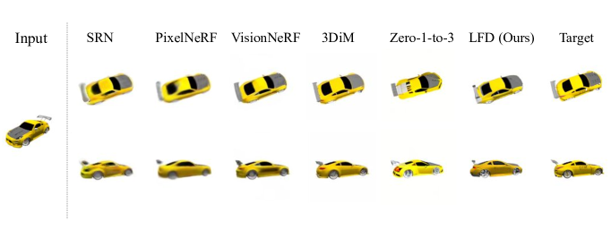
Figure 3: Comparison of Light Field Diffusion and previous works on ShapeNet Car. All results are generated based on a single input. Results of 3DiM [53] come from the official website since 3DiM is not open-source.

Algorithm 1 Training

$\mathcal{I}_{src}$: source image, $\mathcal{I}_{tgt}$: target image, $\mathcal{L}_{src}$: source light field encoding, $\mathcal{L}_{tgt}$: target light field encoding, $T$: timestep, $\alpha_{t}$: fixed variance schedule, $\mathcal{E}$: Encoder, $\mathcal{U}$: U-Net Denoiser

$t\sim$ Uniform($\{1,...,T\}$)

$\epsilon\sim\mathcal{N}(0,I)$

$\{f_{i}\}=\mathcal{E}(\mathcal{I}_{src}\oplus\mathcal{L}_{src})$

$\mathcal{I}_{tgt}^{t}=\sqrt{\bar{\alpha_{t}}}\mathcal{I}_{tgt}+(1-\bar{\alpha_{t}})\epsilon$

Take gradient descent step on

  $\nabla_{\mathcal{U}}||\mathcal{I}_{tgt}-\mathcal{U}(\mathcal{I}_{tgt}^{t},\mathcal{L}_{tgt},\{f_{i}\},t||^{2})$

Until converged

Algorithm 2 Sampling

$\mathcal{I}_{src}$: source image, $\mathcal{L}_{src}$: source light field encoding, $\mathcal{L}_{tgt}$: target light field encoding, $T$: timestep, $\alpha_{t}$: fixed variance schedule, $s$: select refiner timestep, $\mathcal{E}$: Encoder, $\mathcal{U}$: U-Net Denoiser, $\mathcal{R}$: Refiner

$y^{T}\sim\mathcal{N}(0,I)$

$\{f_{i}\}=\mathcal{E}(\mathcal{I}_{src}\oplus\mathcal{L}_{src})$

for $t=T,...,1$ do

     $y^{t-1}=\mathcal{U}(y^{t},\mathcal{L}_{tgt},\{f_{i}\},t)$

end for

$y^{0}=Upsample(y^{0})$

$y^{s}\sim\mathcal{N}(\sqrt{\bar{\alpha_{s}}}y^{0},1-\bar{\alpha_{s}}I)$

for $t=s,...,1$ do

     $y^{t-1}=\mathcal{R}(y^{t},t)$

end for

return $y^{0}$

3.5 Super-resolution Module

The training stage of our approach involves a crucial preprocessing step aimed at standardizing image dimensions for computational efficiency. Specifically, we downsample all images to a uniform size of $64\times 64$. For a fair comparison with other models, we upsample them back to the original size during the evaluation stage. However, a straightforward upsampling process may fall short of preserving the fidelity of the synthesized images.

Thus, we introduce a super-resolution module to upsample the $64\times 64$ image to the original size. The super-resolution module consists of two parts: an upsampling module and a refining module. We train a DDPM [13] as a refiner to enhance the image quality by addressing potential artifacts and imperfections that may arise during the upsampling process. During the inference phase, we add noise to the image and denoise it back.

Empirical experiments conducted to assess the impact of our refinement strategy have yielded compelling results. The incorporation of the DDPM refiner has consistently demonstrated substantial improvements in image quality, effectively bridging the gap between the downsampled results and the desired high-resolution results.

4 Experiments

4.1 Experimental settings

Datasets

We benchmark Light Field Diffusion on ShapeNet Car [3] and Neural 3D Mesh Renderer (NMR) datasets [17]. To remain consistent with other works [53], for ShapeNet Car dataset, we evaluate all test scenes which each has 251 views, and select the 64-th view as the source image. NMR dataset consists of multi-class ShapeNet objects rendered from 24 fixed viewpoints. Following the SRT [37] setting, we use floor division of the scene index by 24 (number of views) to decide the source image. We downsample ShapeNet Car to $64\times 64$ during the training stage, and we upsample the results back to $128\times 128$ for a fair comparison with other models.

Evaluation Metrics

We evaluate our model and prior work using three different metrics: Peak signal-to-noise ratio (PSNR), Structure Similarity Index Measure (SSIM) [52], and Frechet Inception Distance (FID) [12]. PSNR and SSIM are calculated pair to pair with ground truth images and report the average. FID scores are computed with the same number of ground truth views and generated views.

Implementation Details

We train Light Field Diffusion with $T=1000$ noising steps and a linear noise schedule $(1e^{-4}$ to $2e^{-2})$ with a batch size of $64$. We utilize AdamW [22] as the optimizer with an initial learning rate $1e^{-5}$. The training process is performed on a single NVIDIA A6000 GPU. We train Light Field Diffusion for 550k iterations on ShapeNet Car and 580k iterations on the NMR dataset. Same as other diffusion-based models [13, 32], we apply the exponential moving average (EMA) of the U-Net weights with $0.9999$ decay. We adopt the cross-attention layer when the downsampling factor is 4 and 8.

For the super-resolution module, we train a DDPM [13] with $T=1000$ noising steps and a linear noise schedule $(1e^{-4}$ to $2e^{-2})$ as a refiner. We utilize Adam as the optimizer with a learning rate $1e^{-5}$ with a batch size of $64$. The training process is performed on a single NVIDIA A6000 for 350k iterations. We also apply the EMA of the U-Net weights with $0.9999$ decay.

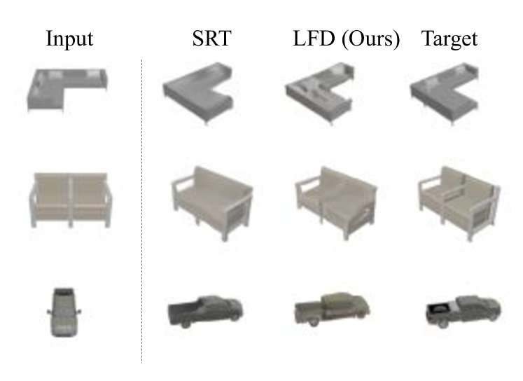
Figure 4: Comparison of Light Field Diffusion and SRT [37] on NMR dataset. Results of Light Field Diffusion are more consistent with the target views. Although SRT has higher PSNR and SSIM, the higher scores come from the blurred results.

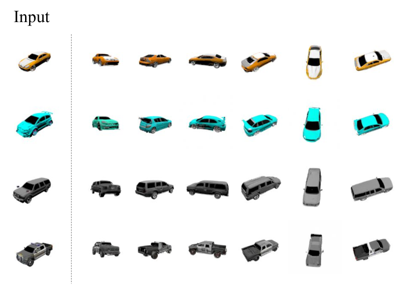
Figure 5: Qualitative ShapeNet Car results. All results are generated based on a single input. We choose 6 different views to present. These results show the 3D consistency of our outputs.

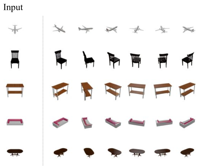
Figure 6: Qualitative NMR results. All results are generated based on a single input. We choose 6 different views to present. These results show the 3D consistency of our outputs.

Method	$\uparrow$ PSNR	$\uparrow$ SSIM	$\downarrow$ FID	Model Size
SRN [40]	22.25	0.88	41.21	70 M
PixelNeRF [57]	23.17	0.89	59.24	28 M
VisionNeRF [20]	22.88	0.90	21.31	125 M
3DiM [53]	21.01	0.57	8.99	471 M
Zero-1-to-3 [21]	19.01	0.84	9.11	860 M
LFD (Ours)	20.17	0.85	12.84	165 M

Table 1: Quantitive ShapeNet Car results. SRN [40], PixelNeRF [57], VisionNeRF [20], and 3DiM [53] baselines are provided by authors of 3DiM [53]. For Zero-1-to-3 [21], we follow the pipeline and downsample the results to $128\times 128$ for comparison. Compared to SRN [40], PixelNeRF [57], and VisionNeRF [20], our method gets a higher FID score. Light Field Diffusion outperforms 3DiM [53] baseline in SSIM and outperforms Zero-1-to-3 [21] baseline in PSNR and SSIM.

4.2 Quantitative Results

We present the quantitative results in Table 1 and Table 2. Since many of the previous works don’t contain FID score, for the NMR dataset, we sample all images of SRT [37] and compute the scores ourselves. For the ShapeNet Car dataset, we use the results from 3DiM [53]. We compare Light Field Diffusion with NeRF-based approach: PixelNeRF [57] and VisionNeRF [20]; Light Field related approach: Scene Representation Transformer [37]; End-to-end diffusion-based approach: 3DiM [53] and Zero 1-to-3 [21]; and Scene Representation Networks[40].

As shown in Table 1 and Table 2, our model achieves competitive results with prior works. Similar to 3DiM [53], our work may not always result in superior reconstruction errors (PSNR and SSIM), but the fidelity of our generated results is significantly better than other regression models. The high PSNR and SSIM scores of regression models may come from blurriness. Since Light Field Diffusion is a generative model, and with only one source image, achieving extremely low reconstruction errors is not realistic.

For the ShapeNet Car dataset, compared to SRN [40], PixelNeRF [57], and VisionNeRF [20], our method gets a higher FID score. Compared to 3DiM [53] and Zero-1-to-3 [21], Light Field Diffusion outperforms 3DiM baseline in SSIM and outperforms Zero-1-to-3 baseline in PSNR and SSIM. For the NMR dataset, Light Field Diffusion outperforms LFN [39] and SRT [37] in FID. We note that Light Field Diffusion is comparably small as a generative model: LFD has only 165M parameters, while 3DiM [53] with $ch=256$ has 471M parameters, and Zero-1-to-3 [21] has 860M parameters.

4.3 Qualitative Results

We also present qualitative results in Figure 5 and Figure 6 to show the 3D consistency of our results. In Figure 3 and Figure 4, we present the qualitative comparison between Light Field Diffusion and other works. For the ShapeNet Car dataset, we compare Light Field Diffusion with SRN [40], PixelNeRF [57], VisionNeRF [20], 3DiM [53], and Zero-1-to-3 [21]. While SRN [40], PixelNeRF [57], and VisionNeRF [20] perform better in PSNR and SSIM in quantitative comparison, the details generated by these models are less consistent with the ground truth. For the NMR dataset, we compare Light Field Diffusion with SRT [37]. Although results produced by SRT match the specific novel viewpoints, this model still has sample quality issues. In contrast, our approach generates novel views that maintain consistency with the source input, ensure viewpoint accuracy, and achieve high quality.

Method	$\uparrow$ PSNR	$\uparrow$ SSIM	$\downarrow$ FID
LFN [39]	24.95	0.87	-
SRT [37]	25.95	0.88	12.53
LFD (Ours)	23.52	0.84	6.93

Table 2: Quantitive NMR results. LFN [39] is provided by the authors (FID for LFN not available). For SRT [37], we use the pipeline and checkpoints provided by a third party since SRT is not open-source. Compared to LFN and SRT, our method gets a higher FID score while maintaining close PSNR and SSIM scores.

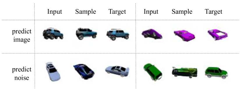
Figure 7: Abalation Study. We show the difference between predicting image and predicting noise. Training the model to predict images produces satisfactory results: the pose corresponds well with the ground truth, albeit the image quality is not flawless. Conversely, when the model is trained to predict noise, it struggles to accurately maintain the pose at this juncture.

4.4 Ablation Study

In the following sections, we present a series of ablation studies concerning Light Field Diffusion, aimed at substantiating the value of the proposed contributions.

Training target

To begin, we delve into the distinction between predicting noise and predicting image, as previously elaborated upon in Section 3. As depicted in Figure 7, under identical conditions and at 21k iterations, training the model to predict images yields reasonable outcomes: the pose aligns with ground truth, although the image quality remains imperfect. However, when trained to predict noise, the model fails to preserve poses accurately at this stage. We can view the light field encoding as a position embedding for each pixel, thus opting to predict the precise value as opposed to the residual (noise) represents a simplistic approach.

Super-resolution

We compare the super-resolution module with a naive upsample algorithm in this study to underscore the significance of refining the image subsequent to its generation. Given that our model is trained using a $64\times 64$ size, employing a basic upsampling technique would result in blurred outcomes. Consequently, the inclusion of a refiner becomes imperative for achieving high image quality. The results are shown in Table 3. With the super-resolution module, our results show improvement in all three metrics.

Refine Step

In this study, we conducted trials with the refiner in super-resolution module using different step counts. For a fair comparison, we start with the same $64\times 64$ low-resolution results. As indicated in Table 4, considering all three metrics – PSNR, SSIM, and FID – the Light Field Diffusion model utilizing a 200-step refiner emerges as the superior. Therefore, we select 200 as the timestep of the refiner in super-resolution module.

Method	$\uparrow$ PSNR	$\uparrow$ SSIM	$\downarrow$ FID
LFD w/ super-resolution module	20.17	0.85	12.84
LFD w/ naive upsample algorithm	20.05	0.83	51.47

Table 3: Abalation Study. We remove the super-resolution module from Light Field Diffusion and instead use a naive upsample algorithm. We can see a huge deterioration in the FID score. The super-resolution module guarantees high image quality.

Method	$\uparrow$ PSNR	$\uparrow$ SSIM	$\downarrow$ FID	Time
LFD w/ 50-steps refiner	20.09	0.83	35.35	1.01s
LFD w/ 100-steps refiner	20.14	0.84	24.84	1.95s
LFD w/ 150-steps refiner	20.17	0.84	16.93	2.91s
LFD w/ 200-steps refiner	20.17	0.85	12.84	3.87s
LFD w/ 300-steps refiner	20.04	0.85	9.55	6.33s

Table 4: Abalation Study. We test several refiners with different steps. With the increase of timesteps, the FID score decreases. But the PSNR score decreases from 200 steps to 300 steps.

5 Conclusion

We propose Light Field Diffusion, an end-to-end conditional diffusion model for single-view novel view synthesis. By capitalizing on the distinct advantages of light field encoding, our proposed light field encoding diffusion model offers a new angle for advancing diffusion models for novel view synthesis. Benefiting from pixel-wise constraints offered by the light field encoding and the cross-attention layer, which combines features extracted from a separate encoder, Light Field Diffusion achieves results that are competitive when compared to other state-of-the-art models across the ShapeNet Car and Neural 3D Mesh Renderer datasets while the model size is only one-third.

Future work includes training Light Field Diffusion on more general datasets, broadening its applicability to a wider range of scenarios. Additionally, we can combine the light field encoding with pre-trained latent diffusion models to unlock even more transformative capabilities. Overall, our work introduces a new possible way for novel view synthesis with diffusion models. We foresee a wider adoption of light fields in generative models for novel view synthesis.

References

- [1] Titas Anciukevičius, Zexiang Xu, Matthew Fisher, Paul Henderson, Hakan Bilen, Niloy J Mitra, and Paul Guerrero. Renderdiffusion: Image diffusion for 3d reconstruction, inpainting and generation. In CVPR, pages 12608–12618, 2023.
- [2] Eric R Chan, Connor Z Lin, Matthew A Chan, Koki Nagano, Boxiao Pan, Shalini De Mello, Orazio Gallo, Leonidas J Guibas, Jonathan Tremblay, Sameh Khamis, et al. Efficient geometry-aware 3d generative adversarial networks. In CVPR, pages 16123–16133, 2022.
- [3] Angel X Chang, Thomas Funkhouser, Leonidas Guibas, Pat Hanrahan, Qixing Huang, Zimo Li, Silvio Savarese, Manolis Savva, Shuran Song, Hao Su, et al. Shapenet: An information-rich 3d model repository. arXiv preprint arXiv:1512.03012, 2015.
- [4] Anpei Chen, Zexiang Xu, Fuqiang Zhao, Xiaoshuai Zhang, Fanbo Xiang, Jingyi Yu, and Hao Su. Mvsnerf: Fast generalizable radiance field reconstruction from multi-view stereo. In CVPR, pages 14124–14133, 2021.
- [5] Shenchang Eric Chen. Quicktime vr: An image-based approach to virtual environment navigation. In SIGGRAPH, pages 29–38, 1995.
- [6] Congyue Deng, Chiyu Jiang, Charles R Qi, Xinchen Yan, Yin Zhou, Leonidas Guibas, Dragomir Anguelov, et al. Nerdi: Single-view nerf synthesis with language-guided diffusion as general image priors. In CVPR, pages 20637–20647, 2023.
- [7] Alexey Dosovitskiy, Lucas Beyer, Alexander Kolesnikov, Dirk Weissenborn, Xiaohua Zhai, Thomas Unterthiner, Mostafa Dehghani, Matthias Minderer, Georg Heigold, Sylvain Gelly, et al. An image is worth 16x16 words: Transformers for image recognition at scale. ICLR, 2010.
- [8] John Flynn, Michael Broxton, Paul Debevec, Matthew DuVall, Graham Fyffe, Ryan Overbeck, Noah Snavely, and Richard Tucker. Deepview: View synthesis with learned gradient descent. In CVPR, pages 2367–2376, 2019.
- [9] Ian Goodfellow, Jean Pouget-Abadie, Mehdi Mirza, Bing Xu, David Warde-Farley, Sherjil Ozair, Aaron Courville, and Yoshua Bengio. Generative adversarial nets. In NIPS, 2014.
- [10] Jiatao Gu, Lingjie Liu, Peng Wang, and Christian Theobalt. Stylenerf: A style-based 3d-aware generator for high-resolution image synthesis. ICLR, 2022.
- [11] Jiatao Gu, Alex Trevithick, Kai-En Lin, Josh Susskind, Christian Theobalt, Lingjie Liu, and Ravi Ramamoorthi. Nerfdiff: Single-image view synthesis with nerf-guided distillation from 3d-aware diffusion. In ICML, 2023.
- [12] Martin Heusel, Hubert Ramsauer, Thomas Unterthiner, Bernhard Nessler, and Sepp Hochreiter. Gans trained by a two time-scale update rule converge to a local nash equilibrium. Advances in neural information processing systems, 30, 2017.
- [13] Jonathan Ho, Ajay Jain, and Pieter Abbeel. Denoising diffusion probabilistic models. NIPS, 33:6840–6851, 2020.
- [14] Ajay Jain, Matthew Tancik, and Pieter Abbeel. Putting nerf on a diet: Semantically consistent few-shot view synthesis. In CVPR, pages 5885–5894, 2021.
- [15] Wonbong Jang and Lourdes Agapito. Codenerf: Disentangled neural radiance fields for object categories. In CVPR, pages 12949–12958, 2021.
- [16] Tero Karras, Samuli Laine, and Timo Aila. A style-based generator architecture for generative adversarial networks. In CVPR, pages 4401–4410, 2019.
- [17] Hiroharu Kato, Yoshitaka Ushiku, and Tatsuya Harada. Neural 3d mesh renderer. In CVPR, pages 3907–3916, 2018.
- [18] Diederik Kingma, Tim Salimans, Ben Poole, and Jonathan Ho. Variational diffusion models. NIPS, 34:21696–21707, 2021.
- [19] Marc Levo and Pat Hanrahan. Light field rendering. 1996.
- [20] Kai-En Lin, Yen-Chen Lin, Wei-Sheng Lai, Tsung-Yi Lin, Yi-Chang Shih, and Ravi Ramamoorthi. Vision transformer for nerf-based view synthesis from a single input image. In WACV, pages 806–815, 2023.
- [21] Ruoshi Liu, Rundi Wu, Basile Van Hoorick, Pavel Tokmakov, Sergey Zakharov, and Carl Vondrick. Zero-1-to-3: Zero-shot one image to 3d object, 2023.
- [22] Ilya Loshchilov and Frank Hutter. Decoupled weight decay regularization. In ICLR, 2019.
- [23] Ben Mildenhall, Pratul P Srinivasan, Matthew Tancik, Jonathan T Barron, Ravi Ramamoorthi, and Ren Ng. Nerf: Representing scenes as neural radiance fields for view synthesis. Communications of the ACM, 65(1):99–106, 2021.
- [24] Norman Müller, Yawar Siddiqui, Lorenzo Porzi, Samuel Rota Bulo, Peter Kontschieder, and Matthias Nießner. Diffrf: Rendering-guided 3d radiance field diffusion. In CVPR, pages 4328–4338, 2023.
- [25] Przemyslaw Musialski, Peter Wonka, Daniel G Aliaga, Michael Wimmer, Luc Van Gool, and Werner Purgathofer. A survey of urban reconstruction. In Computer graphics forum, pages 146–177. Wiley Online Library, 2013.
- [26] Alex Nichol, Prafulla Dhariwal, Aditya Ramesh, Pranav Shyam, Pamela Mishkin, Bob McGrew, Ilya Sutskever, and Mark Chen. Glide: Towards photorealistic image generation and editing with text-guided diffusion models. arXiv preprint arXiv:2112.10741, 2021.
- [27] Michael Niemeyer, Jonathan T Barron, Ben Mildenhall, Mehdi SM Sajjadi, Andreas Geiger, and Noha Radwan. Regnerf: Regularizing neural radiance fields for view synthesis from sparse inputs. In Proceedings of the IEEE/CVF Conference on Computer Vision and Pattern Recognition, pages 5480–5490, 2022.
- [28] Michael Niemeyer and Andreas Geiger. Giraffe: Representing scenes as compositional generative neural feature fields. In Proceedings of the IEEE/CVF Conference on Computer Vision and Pattern Recognition, pages 11453–11464, 2021.
- [29] Eunbyung Park, Jimei Yang, Ersin Yumer, Duygu Ceylan, and Alexander C Berg. Transformation-grounded image generation network for novel 3d view synthesis. In CVPR, pages 3500–3509, 2017.
- [30] Sida Peng, Yuanqing Zhang, Yinghao Xu, Qianqian Wang, Qing Shuai, Hujun Bao, and Xiaowei Zhou. Neural body: Implicit neural representations with structured latent codes for novel view synthesis of dynamic humans. In CVPR, pages 9054–9063, 2021.
- [31] Alec Radford, Jong Wook Kim, Chris Hallacy, Aditya Ramesh, Gabriel Goh, Sandhini Agarwal, Girish Sastry, Amanda Askell, Pamela Mishkin, Jack Clark, et al. Learning transferable visual models from natural language supervision. In ICML, pages 8748–8763. PMLR, 2021.
- [32] Robin Rombach, Andreas Blattmann, Dominik Lorenz, Patrick Esser, and Björn Ommer. High-resolution image synthesis with latent diffusion models. In CVPR, pages 10684–10695, 2022.
- [33] Robin Rombach, Patrick Esser, and Björn Ommer. Geometry-free view synthesis: Transformers and no 3d priors. In ICCV, pages 14356–14366, 2021.
- [34] Olaf Ronneberger, Philipp Fischer, and Thomas Brox. U-net: Convolutional networks for biomedical image segmentation. In MICCAI, pages 234–241. Springer, 2015.
- [35] Chitwan Saharia, William Chan, Huiwen Chang, Chris Lee, Jonathan Ho, Tim Salimans, David Fleet, and Mohammad Norouzi. Palette: Image-to-image diffusion models. In SIGGRAPH, pages 1–10, 2022.
- [36] Chitwan Saharia, William Chan, Saurabh Saxena, Lala Li, Jay Whang, Emily L Denton, Kamyar Ghasemipour, Raphael Gontijo Lopes, Burcu Karagol Ayan, Tim Salimans, et al. Photorealistic text-to-image diffusion models with deep language understanding. NIPS, 35:36479–36494, 2022.
- [37] Mehdi SM Sajjadi, Henning Meyer, Etienne Pot, Urs Bergmann, Klaus Greff, Noha Radwan, Suhani Vora, Mario Lučić, Daniel Duckworth, Alexey Dosovitskiy, et al. Scene representation transformer: Geometry-free novel view synthesis through set-latent scene representations. In CVPR, pages 6229–6238, 2022.
- [38] Katja Schwarz, Yiyi Liao, Michael Niemeyer, and Andreas Geiger. Graf: Generative radiance fields for 3d-aware image synthesis. NeurIPS, 33:20154–20166, 2020.
- [39] Vincent Sitzmann, Semon Rezchikov, William T. Freeman, Joshua B. Tenenbaum, and Fredo Durand. Light field networks: Neural scene representations with single-evaluation rendering. In NeurIPS, 2021.
- [40] Vincent Sitzmann, Michael Zollhöfer, and Gordon Wetzstein. Scene representation networks: Continuous 3d-structure-aware neural scene representations. Advances in Neural Information Processing Systems, 32, 2019.
- [41] Jascha Sohl-Dickstein, Eric Weiss, Niru Maheswaranathan, and Surya Ganguli. Deep unsupervised learning using nonequilibrium thermodynamics. In ICML, pages 2256–2265. PMLR, 2015.
- [42] Yang Song, Conor Durkan, Iain Murray, and Stefano Ermon. Maximum likelihood training of score-based diffusion models. Advances in Neural Information Processing Systems, 34:1415–1428, 2021.
- [43] Yang Song and Stefano Ermon. Generative modeling by estimating gradients of the data distribution. Advances in neural information processing systems, 32, 2019.
- [44] Yang Song, Jascha Sohl-Dickstein, Diederik P Kingma, Abhishek Kumar, Stefano Ermon, and Ben Poole. Score-based generative modeling through stochastic differential equations. In ICLR, 2021.
- [45] Mohammed Suhail, Carlos Esteves, Leonid Sigal, and Ameesh Makadia. Generalizable patch-based neural rendering. In ECCV, pages 156–174, 2022.
- [46] Mohammed Suhail, Carlos Esteves, Leonid Sigal, and Ameesh Makadia. Light field neural rendering. In CVPR, pages 8269–8279, 2022.
- [47] Shao-Hua Sun, Minyoung Huh, Yuan-Hong Liao, Ning Zhang, and Joseph J Lim. Multi-view to novel view: Synthesizing novel views with self-learned confidence. In ECCV, pages 155–171, 2018.
- [48] Richard Szeliski and Heung-Yeung Shum. Creating full view panoramic image mosaics and environment maps. In SIGGRAPH, pages 653–660. 2023.
- [49] Edgar Tretschk, Ayush Tewari, Vladislav Golyanik, Michael Zollhöfer, Christoph Lassner, and Christian Theobalt. Non-rigid neural radiance fields: Reconstruction and novel view synthesis of a dynamic scene from monocular video. In CVPR, pages 12959–12970, 2021.
- [50] Alex Trevithick and Bo Yang. Grf: Learning a general radiance field for 3d representation and rendering. In Proceedings of the IEEE/CVF International Conference on Computer Vision, pages 15182–15192, 2021.
- [51] Hung-Yu Tseng, Qinbo Li, Changil Kim, Suhib Alsisan, Jia-Bin Huang, and Johannes Kopf. Consistent view synthesis with pose-guided diffusion models. In CVPR, pages 16773–16783, 2023.
- [52] Zhou Wang, Alan C Bovik, Hamid R Sheikh, and Eero P Simoncelli. Image quality assessment: from error visibility to structural similarity. IEEE transactions on image processing, 13(4):600–612, 2004.
- [53] Daniel Watson, William Chan, Ricardo Martin-Brualla, Jonathan Ho, Andrea Tagliasacchi, and Mohammad Norouzi. Novel view synthesis with diffusion models. ICLR, 2022.
- [54] Jamie Wynn and Daniyar Turmukhambetov. Diffusionerf: Regularizing neural radiance fields with denoising diffusion models. In CVPR, pages 4180–4189, 2023.
- [55] Dejia Xu, Yifan Jiang, Peihao Wang, Zhiwen Fan, Humphrey Shi, and Zhangyang Wang. Sinnerf: Training neural radiance fields on complex scenes from a single image. In ECCV, pages 736–753. Springer, 2022.
- [56] Dejia Xu, Yifan Jiang, Peihao Wang, Zhiwen Fan, Yi Wang, and Zhangyang Wang. Neurallift-360: Lifting an in-the-wild 2d photo to a 3d object with 360deg views. In CVPR, pages 4479–4489, 2023.
- [57] Alex Yu, Vickie Ye, Matthew Tancik, and Angjoo Kanazawa. pixelnerf: Neural radiance fields from one or few images. In CVPR, pages 4578–4587, 2021.
- [58] Tinghui Zhou, Richard Tucker, John Flynn, Graham Fyffe, and Noah Snavely. Stereo magnification: Learning view synthesis using multiplane images. In SIGGRAPH, 2018.
- [59] Zhizhuo Zhou and Shubham Tulsiani. Sparsefusion: Distilling view-conditioned diffusion for 3d reconstruction. In CVPR, pages 12588–12597, 2023.
- [60] Xinge Zhu, Zhichao Yin, Jianping Shi, Hongsheng Li, and Dahua Lin. Generative adversarial frontal view to bird view synthesis. In 3DV, pages 454–463. IEEE, 2018.