RMT: Retentive Networks Meet Vision Transformers

Abstract

Vision Transformer (ViT) has gained increasing attention in the computer vision community in recent years. However, the core component of ViT, Self-Attention, lacks explicit spatial priors and bears a quadratic computational complexity, thereby constraining the applicability of ViT. To alleviate these issues, we draw inspiration from the recent Retentive Network (RetNet) in the field of NLP, and propose RMT, a strong vision backbone with explicit spatial prior for general purposes. Specifically, we extend the RetNet’s temporal decay mechanism to the spatial domain, and propose a spatial decay matrix based on the Manhattan distance to introduce the explicit spatial prior to Self-Attention. Additionally, an attention decomposition form that adeptly adapts to explicit spatial prior is proposed, aiming to reduce the computational burden of modeling global information without disrupting the spatial decay matrix. Based on the spatial decay matrix and the attention decomposition form, we can flexibly integrate explicit spatial prior into the vision backbone with linear complexity. Extensive experiments demonstrate that RMT exhibits exceptional performance across various vision tasks. Specifically, without extra training data, RMT achieves 84.8% and 86.1% top-1 acc on ImageNet-1k with 27M/4.5GFLOPs and 96M/18.2GFLOPs. For downstream tasks, RMT achieves 54.5 box AP and 47.2 mask AP on the COCO detection task, and 52.8 mIoU on the ADE20K semantic segmentation task. Code is available at https://github.com/qhfan/RMT

1 Introduction

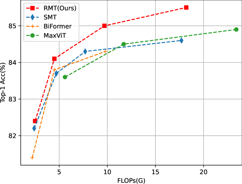
Model	#Params	Top1 Acc.
MaxViT-T [31]	31M	83.6
SMT-S [34]	20M	83.7
BiFormer-S [75]	26M	83.8
RMT-S (Ours)	27M	84.1
RMT-S* (Ours)	27M	84.8
BiFormer-B [75]	57M	84.3
MaxViT-S [29]	69M	84.5
RMT-B (Ours)	54M	85.0
RMT-B* (Ours)	55M	85.6
SMT-L [34]	81M	84.6
MaxViT-B [51]	120M	84.9
RMT-L (Ours)	95M	85.5
RMT-L* (Ours)	96M	86.1

Figure 1: FLOPs v.s. Top-1 accuracy on ImageNet-1K with $224\times 224$ resolution. “*” indicates the model trained with token labeling [27].

Vision Transformer (ViT) [12] is an excellent visual architecture highly favored by researchers. However, as the core module of ViT, Self-Attention’s inherent structure lacking explicit spatial priors. Besides, the quadratic complexity of Self-Attention leads to significant computational costs when modeling global information. These issues limit the application of ViT.

Many works have previously attempted to alleviate these issues [30, 35, 50, 13, 57, 16, 61]. For example, in Swin Transformer [35], the authors partition the tokens used for self-attention by applying windowing operations. This operation not only reduces the computational cost of self-attention but also introduces spatial priors to the model through the use of windows and relative position encoding. In addition to it, NAT [19] changes the receptive field of Self-Attention to match the shape of convolution, reducing computational costs while also enabling the model to perceive spatial priors through the shape of its receptive field.

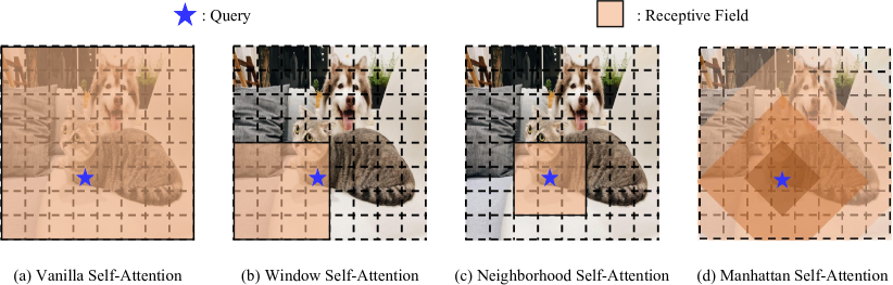
Figure 2: Comparison among different Self-Attention mechanisms. In MaSA, darker colors represent smaller spatial decay rates, while lighter colors represent larger ones. The spatial decay rates that change with distance provide the model with rich spatial priors.

Different from previous methods, we draw inspiration from the recently successful Retentive Network (RetNet) [46] in the field of NLP. RetNet utilizes a distance-dependent temporal decay matrix to provide explicit temporal prior for one-dimensional and unidirectional text data. ALiBi [41], prior to RetNet, also applied a similar approach and succeeded in NLP tasks. We extend this temporal decay matrix to the spatial domain, developing a two-dimensional bidirectional spatial decay matrix based on the Manhattan distance among tokens. In our space decay matrix, for a target token, the farther the surrounding tokens are, the greater the degree of decay in their attention scores. This property allows the target token to perceive global information while simultaneously assigning different levels of attention to tokens at varying distances. We introduce explicit spatial prior to the vision backbone using this spatial decay matrix. We name this Self-Attention mechanism, which is inspired by RetNet and incorporates the Manhattan distance as the explicit spatial prior, as Manhattan Self-Attention (MaSA).

Besides explicit spatial priors, another issue caused by global modeling with Self-Attention is the enormous computational burden. Previous sparse attention mechanisms [11, 35, 53, 63, 75] and the way retention is decomposed in RetNet [46] mostly disrupt the spatial decay matrix, making them unsuitable for MaSA. In order to sparsely model global information without compromising the spatial decay matrix, we propose a method to decompose Self-Attention along both axes of the image. This decomposition method decomposes Self-Attention and the spatial decay matrix without any loss of prior information. The decomposed MaSA models global information with linear complexity and has the same receptive field shape as the original MaSA. We compare MaSA with other Self-Attention mechanisms in Fig. 2. It can be seen that our MaSA introduces richer spatial priors to the model than its counterparts.

Based on MaSA, we construct a powerful vision backbone called RMT. We demonstrate the effectiveness of the proposed method through extensive experiments. As shown in Fig. 1, our RMT outperforms the state-of-the-art (SOTA) models on image classification tasks. Additionally, our model exhibits more prominent advantages compared to other models in tasks such as object detection, instance segmentation, and semantic segmentation. Our contributions can be summarized as follows:

• We propose a spatial decay matrix based on Manhattan distance to augment Self-Attention, creating the Manhattan Self-Attention (MaSA) with an explicit spatial prior.

• We propose a decomposition form for MaSA, enabling linear complexity for global information modeling without disrupting the spatial decay matrix.

• Leveraging MaSA, we construct RMT, a powerful vision backbone for general purposes. RMT attains high top-1 accuracy on ImageNet-1k in image classification without extra training data, and excels in tasks like object detection, instance segmentation, and semantic segmentation.

2 Related Work

Transformer.

Transformer architecture was firstly proposed in [52] to address the training limitation of recurrent model and then achieve massive success in many NLP tasks. By splitting the image into small, non-overlapped patches sequence, Vision Transformer (ViTs) [12] also have attracted great attention and become widely used on vision tasks [66, 18, 58, 14, 39, 5]. Unlike in the past, where RNNs and CNNs have respectively dominated the NLP and CV fields, the transformer architecture has shined through in various modalities and fields [37, 60, 42, 26]. In the computer vision community, many studies are attempting to introduce spatial priors into ViT to reduce the data requirements for training [6, 49, 19]. At the same time, various sparse attention mechanisms have been proposed to reduce the computational cost of Self-Attention [53, 54, 13, 57].

Prior Knowledge in Transformer.

Numerous attempts have been made to incorporate prior knowledge into the Transformer model to enhance its performance. The original Transformers [12, 52] use trigonometric position encoding to provide positional information for each token. In vision tasks, [35] proposes the use of relative positional encoding as a replacement for the original absolute positional encoding. [6] points out that zero padding in convolutional layers could also provide positional awareness for the ViT, and this position encoding method is highly efficient. In many studies, Convolution in FFN [16, 54, 13] has been employed for vision models to further enrich the positional information in the ViT. For NLP tasks, in the recent Retentive Network [46], the temporal decay matrix has been introduced to provide the model with prior knowledge based on distance changes. Before RetNet, ALiBi [41] also uses a similar temporal decay matrix.

3 Methodology

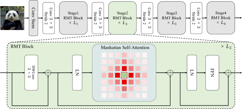
Figure 3: Overall architecture of RMT.

3.1 Preliminary

Temporal decay in RetNet.

Retentive Network (RetNet) is a powerful architecture for language models. This work proposes the retention mechanism for sequence modeling. Retention brings the temporal decay to the language model, which Transformers do not have. Retention firstly considers a sequence modeling problem in a recurrent manner. It can be written as Eq. 1:

$$o_{n}=\sum_{m=1}^{n}\gamma^{n-m}(Q_{n}e^{in\theta})(K_{m}e^{im\theta})^{\dagger}v_{m}$$ (1)

For a parallel training process, Eq. 1 is expressed as:

$$Q=(XW_{Q})\odot\Theta, \quad K=(XW_{K})\odot\overline{\Theta},\quad V=XW_{V}$$ (2)

$$\Theta_{n}=e^{in\theta}, \quad D_{nm}=\left\{\begin{aligned} &\gamma^{n-m},&n\geq m\\ &0,&n<m\\ \end{aligned}\right.$$

$$\mathrm{Rete} \mathrm{ntion}(X)=(QK^{\intercal}\odot D)V$$

where $\overline{\Theta}$ is the complex conjugate of $\Theta$, and $D\in\mathbb{R}^{|x|\times|x|}$ contains both causal masking and exponential decay, which symbolizes the relative distance in one-dimensional sequence and brings the explicit temporal prior to text data.

3.2 Manhattan Self-Attention

Starting from the retention in RetNet, we evolve it into Manhattan Self-Attention (MaSA). Within MaSA, we transform the unidirectional and one-dimensional temporal decay observed in retention into bidirectional and two-dimensional spatial decay. This spatial decay introduces an explicit spatial prior linked to Manhattan distance into the vision backbone. Additionally, we devise a straightforward approach to concurrently decompose the Self-Attention and spatial decay matrix along the two axes of the image.

From Unidirectional to Bidirectional Decay:

In RetNet, retention is unidirectional due to the causal nature of text data, allowing each token to attend only to preceding tokens and not those following it. This characteristic is ill-suited for tasks lacking causal properties, such as image recognition. Hence, we initially broaden the retention to a bidirectional form, expressed as Eq. 3:

$$\mathrm{BiRetention}(X) =(QK^{\intercal}\odot D^{Bi})V$$ (3)

$$D_{nm}^{Bi} =\gamma^{|n-m|}$$

where $\mathrm{BiRetention}$ signifies bidirectional modeling.

From One-dimensional to Two-dimensional Decay:

While retention now supports bi-directional modeling, this capability remains confined to a one-dimensional level and is inadequate for two-dimensional images. To address this limitation, we extend the one-dimensional retention to encompass two dimensions.

In the context of images, each token is uniquely positioned with a two-dimensional coordinate within the plane, denoted as $(x_{n},y_{n})$ for the $n$-th token. To adapt to this, we adjust each element in the matrix $D$ to represent the Manhattan distance between the respective token pairs based on their 2D coordinates. The matrix $D$ is redefined as follows:

$$D_{nm}^{2d}=\gamma^{|x_{n}-x_{m}|+|y_{n}-y_{m}|}$$ (4)

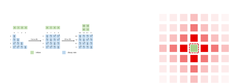
Figure 4: Spatial decay matrix in the decomposed MaSA.

In the retention, the $\mathrm{Softmax}$ is abandoned and replaced with a gating function. This variation gives RetNet multiple flexible computation forms, enabling it to adapt to parallel training and recurrent inference processes. Despite this flexibility, when exclusively utilizing RetNet’s parallel computation form in our experiments, the necessity of retaining the gating function becomes debatable. Our findings indicate that this modification does not improve results for vision models; instead, it introduces extra parameters and computational complexity. Consequently, we continue to employ $\mathrm{Softmax}$ to introduce nonlinearity to our model. Combining the aforementioned steps, our Manhattan Self-Attention is expressed as

$$\mathrm{MaSA}(X) =(\mathrm{Softmax}(QK^{\intercal})\odot D^{2d})V$$ (5)

$$D_{nm}^{2d} =\gamma^{|x_{n}-x_{m}|+|y_{n}-y_{m}|}$$

Decomposed Manhattan Self-Attention.

In the early stages of the vision backbone, an abundance of tokens leads to high computational costs for Self-Attention when attempting to model global information. Our MaSA encounters this challenge as well. Utilizing existing sparse attention mechanisms [35, 11, 19, 53, 63], or the original RetNet’s recurrent/chunk-wise recurrent form directly, disrupts the spatial decay matrix based on Manhattan distance, resulting in the loss of explicit spatial prior. To address this, we introduce a simple decomposition method that not only decomposes Self-Attention but also decomposes the spatial decay matrix. The decomposed MaSA is represented in Eq. 6. Specifically, we calculate attention scores separately for the horizontal and vertical directions in the image. Subsequently, we apply the one-dimensional bidirectional decay matrix to these attention weights. The one-dimensional decay matrix signifies the horizontal and vertical distances between tokens ($D^{H}_{nm}=\gamma^{|y_{n}-y_{m}|}$, $D^{W}_{nm}=\gamma^{|x_{n}-x_{m}|}$):

$$Attn_{H}=\mathrm{Softmax}(Q_{H}K_{H}^{\intercal})\odot D^{H},$$ (6)

$$Attn_{W}=\mathrm{Softmax}(Q_{W}K_{W}^{\intercal})\odot D^{W},$$

$$\mathrm{MaSA}(X)=Attn_{H}(Attn_{W}V)^{\intercal}$$

Based on the decomposition of MaSA, the shape of the receptive field of each token is shown in Fig. 4, which is identical to the shape of the complete MaSA’s receptive field. Fig. 4 indicates that our decomposition method fully preserves the explicit spatial prior.

Cost	Model	Parmas (M)	FLOPs (G)	Top1-acc (%)
tiny model $\sim 2.5$G	PVTv2-b1 [54]	13	2.1	78.7
	QuadTree-B-b1 [48]	14	2.3	80.0
	RegionViT-T [3]	14	2.4	80.4
	MPViT-XS [29]	11	2.9	80.9
	tiny-MOAT-2 [62]	10	2.3	81.0
	VAN-B1 [17]	14	2.5	81.1
	BiFormer-T [75]	13	2.2	81.4
	Conv2Former-N [23]	15	2.2	81.5
	CrossFormer-T [55]	28	2.9	81.5
	NAT-M [19]	20	2.7	81.8
	QnA-T [1]	16	2.5	82.0
	GC-ViT-XT [20]	20	2.6	82.0
	SMT-T [34]	12	2.4	82.2
	RMT-T	14	2.5	82.4
small model $\sim 4.5$G	DeiT-S [49]	22	4.6	79.9
	Swin-T [35]	29	4.5	81.3
	ConvNeXt-T [36]	29	4.5	82.1
	Focal-T [63]	29	4.9	82.2
	FocalNet-T [64]	29	4.5	82.3
	RegionViT-S [3]	31	5.3	82.6
	CSWin-T [11]	23	4.3	82.7
	MPViT-S [29]	23	4.7	83.0
	ScalableViT-S [65]	32	4.2	83.1
	SG-Former-S [15]	23	4.8	83.2
	MOAT-0 [62]	28	5.7	83.3
	Ortho-S [25]	24	4.5	83.4
	InternImage-T [56]	30	5.0	83.5
	CMT-S [16]	25	4.0	83.5
	MaxViT-T [51]	31	5.6	83.6
	SMT-S [34]	20	4.8	83.7
	BiFormer-S [75]	26	4.5	83.8
	RMT-S	27	4.5	84.1
	LV-ViT-S* [27]	26	6.6	83.3
	UniFormer-S* [30]	24	4.2	83.4
	WaveViT-S* [66]	23	4.7	83.9
	Dual-ViT-S* [67]	25	5.4	84.1
	VOLO-D1* [68]	27	6.8	84.2
	BiFormer-S* [75]	26	4.5	84.3
	RMT-S*	27	4.5	84.8

(a)

Cost	Model	Parmas (M)	FLOPs (G)	Top1-acc (%)
base model $\sim 9.0$G	Swin-S [35]	50	8.7	83.0
	ConvNeXt-S [36]	50	8.7	83.1
	CrossFormer-B [55]	52	9.2	83.4
	NAT-S [19]	51	7.8	83.7
	Quadtree-B-b4 [48]	64	11.5	84.0
	Ortho-B [25]	50	8.6	84.0
	ScaleViT-B [65]	81	8.6	84.1
	MOAT-1 [62]	42	9.1	84.2
	InternImage-S [56]	50	8.0	84.2
	DaViT-S [10]	50	8.8	84.2
	GC-ViT-S [20]	51	8.5	84.3
	BiFormer-B [75]	57	9.8	84.3
	MViTv2-B [31]	52	10.2	84.4
	iFormer-B [45]	48	9.4	84.6
	RMT-B	54	9.7	85.0
	WaveViT-B* [66]	34	7.2	84.8
	UniFormer-B* [30]	50	8.3	85.1
	Dual-ViT-B* [67]	43	9.3	85.2
	BiFormer-B* [75]	58	9.8	85.4
	RMT-B*	55	9.7	85.6
large model $\sim 18.0$G	Swin-B [35]	88	15.4	83.3
	CaiT-M24 [50]	186	36	83.4
	LITv2 [39]	87	13.2	83.6
	CrossFormer-L [55]	92	16.1	84.0
	Ortho-L [25]	88	15.4	84.2
	CSwin-B [11]	78	15.0	84.2
	SMT-L [34]	81	17.7	84.6
	MOAT-2 [62]	73	17.2	84.7
	SG-Former-B [15]	78	15.6	84.7
	iFormer-L [45]	87	14.0	84.8
	InterImage-B [56]	97	16.0	84.9
	MaxViT-B [51]	120	23.4	84.9
	GC-ViT-B [20]	90	14.8	85.0
	RMT-L	95	18.2	85.5
	VOLO-D3* [68]	86	20.6	85.4
	WaveViT-L* [66]	58	14.8	85.5
	UniFormer-L* [30]	100	12.6	85.6
	Dual-ViT-L* [67]	73	18.0	85.7
	RMT-L*	96	18.2	86.1

(b)

Table 1: Comparison with the state-of-the-art on ImageNet-1K classification. “*” indicates the model trained with token labeling [27].

To further enhance the local expression capability of MaSA, following [75], we introduce a Local Context Enhancement module using DWConv:

$$X_{out}=\mathrm{MaSA}(X)+\mathrm{LCE}(V);$$ (7)

3.3 Overall Architecture

We construct the RMT based on MaSA, and its architecture is illustrated in Fig. 3. Similar to previous general vision backbones [53, 54, 35, 71], RMT is divided into four stages. The first three stages utilize the decomposed MaSA, while the last uses the original MaSA. Like many previous backbones [16, 75, 30, 72], we incorporate CPE [6] into our model.

Backbone	Params (M)	FLOPs (G)	Mask R-CNN $1\times$						Params (M)	FLOPs (G)	RetinaNet $1\times$
			$AP^{b}$	$AP^{b}_{50}$	$AP^{b}_{75}$	$AP^{m}$	$AP^{m}_{50}$	$AP^{m}_{75}$			$AP^{b}$	$AP^{b}_{50}$	$AP^{b}_{75}$	$AP^{b}_{S}$	$AP^{b}_{M}$	$AP^{b}_{L}$
PVT-T [53]	33	240	39.8	62.2	43.0	37.4	59.3	39.9	23	221	39.4	59.8	42.0	25.5	42.0	52.1
PVTv2-B1 [54]	33	243	41.8	54.3	45.9	38.8	61.2	41.6	23	225	41.2	61.9	43.9	25.4	44.5	54.3
MPViT-XS [29]	30	231	44.2	66.7	48.4	40.4	63.4	43.4	20	211	43.8	65.0	47.1	28.1	47.6	56.5
RMT-T	33	218	47.1	68.8	51.7	42.6	65.8	45.9	23	199	45.1	66.2	48.1	28.8	48.9	61.1
Swin-T [35]	48	267	43.7	66.6	47.7	39.8	63.3	42.7	38	248	41.7	63.1	44.3	27.0	45.3	54.7
CMT-S [16]	45	249	44.6	66.8	48.9	40.7	63.9	43.4	44	231	44.3	65.5	47.5	27.1	48.3	59.1
CrossFormer-S [55]	50	301	45.4	68.0	49.7	41.4	64.8	44.6	41	272	44.4	65.8	47.4	28.2	48.4	59.4
ScalableViT-S [65]	46	256	45.8	67.6	50.0	41.7	64.7	44.8	36	238	45.2	66.5	48.4	29.2	49.1	60.3
MPViT-S [29]	43	268	46.4	68.6	51.2	42.4	65.6	45.7	32	248	45.7	57.3	48.8	28.7	49.7	59.2
CSWin-T [11]	42	279	46.7	68.6	51.3	42.2	65.6	45.4	–	–	–	–	–	–	–	–
InternImage-T [56]	49	270	47.2	69.0	52.1	42.5	66.1	45.8	–	–	–	–	–	–	–	–
SMT-S [34]	40	265	47.8	69.5	52.1	43.0	66.6	46.1	–	–	–	–	–	–	–	–
BiFormer-S [75]	–	–	47.8	69.8	52.3	43.2	66.8	46.5	–	–	45.9	66.9	49.4	30.2	49.6	61.7
RMT-S	46	262	49.0	70.8	53.9	43.9	67.8	47.4	36	244	47.8	69.1	51.8	32.1	51.8	63.5
ResNet-101 [21]	63	336	40.4	61.1	44.2	36.4	57.7	38.8	58	315	38.5	57.8	41.2	21.4	42.6	51.1
Swin-S [35]	69	359	45.7	67.9	50.4	41.1	64.9	44.2	60	339	44.5	66.1	47.4	29.8	48.5	59.1
ScalableViT-B [65]	95	349	46.8	68.7	51.5	42.5	65.8	45.9	85	330	45.8	67.3	49.2	29.9	49.5	61.0
InternImage-S [56]	69	340	47.8	69.8	52.8	43.3	67.1	46.7	–	–	–	–	–	–	–	–
CSWin-S [11]	54	342	47.9	70.1	52.6	43.2	67.1	46.2	–	–	–	–	–	–	–	–
BiFormer-B [75]	–	–	48.6	70.5	53.8	43.7	67.6	47.1	–	–	47.1	68.5	50.4	31.3	50.8	62.6
RMT-B	73	373	51.1	72.5	56.1	45.5	69.7	49.3	63	355	49.1	70.3	53.0	32.9	53.2	64.2
Swin-B [35]	107	496	46.9	69.2	51.6	42.3	66.0	45.5	98	477	45.0	66.4	48.3	28.4	49.1	60.6
PVTv2-B5 [54]	102	557	47.4	68.6	51.9	42.5	65.7	46.0	–	–	–	–	–	–	–	–
Focal-B [63]	110	533	47.8	70.2	52.5	43.2	67.3	46.5	101	514	46.3	68.0	49.8	31.7	50.4	60.8
MPViT-B [29]	95	503	48.2	70.0	52.9	43.5	67.1	46.8	85	482	47.0	68.4	50.8	29.4	51.3	61.5
CSwin-B [11]	97	526	48.7	70.4	53.9	43.9	67.8	47.3	–	–	–	–	–	–	–	–
InternImage-B [56]	115	501	48.8	70.9	54.0	44.0	67.8	47.4	–	–	–	–	–	–	–	–
RMT-L	114	557	51.6	73.1	56.5	45.9	70.3	49.8	104	537	49.4	70.6	53.1	34.2	53.9	65.2

Table 2: Comparison to other backbones using RetinaNet and Mask R-CNN on COCO val2017 object detection and instance segmentation.

4 Experiments

We conducted extensive experiments on multiple vision tasks, such as image classification on ImageNet-1K [9], object detection and instance segmentation on COCO 2017 [33], and semantic segmentation on ADE20K [74]. We also make ablation studies to validate the importance of each component in RMT. More details can be found in Appendix.

4.1 Image Classification

Settings.

We train our models on ImageNet-1K [9] from scratch. We follow the same training strategy in [49], with the only supervision being classification loss for a fair comparison. The maximum rates of increasing stochastic depth [24] are set to 0.1/0.15/0.4/0.5 for RMT-T/S/B/L [24], respectively. We use the AdamW optimizer with a cosine decay learning rate scheduler to train the models. We set the initial learning rate, weight decay, and batch size to 0.001, 0.05, and 1024, respectively. We adopt the strong data augmentation and regularization used in [35]. Our settings are RandAugment [8] (randm9-mstd0.5-inc1), Mixup [70] (prob=0.8), CutMix [69] (prob=1.0), Random Erasing [73] (prob=0.25). In addition to the conventional training methods, similar to LV-ViT [27] and VOLO [68], we train a model that utilizes token labeling to provide supplementary supervision.

Results.

We compare RMT against many state-of-the-art models in Tab. 1. Results in the table demonstrate that RMT consistently outperforms previous models across all settings. Specifically, RMT-S achieves 84.1% Top1-accuracy with only 4.5 GFLOPs. RMT-B also surpasses iFormer [45] by 0.4% with similar FLOPs. Furthermore, our RMT-L model surpasses MaxViT-B [51] in top1-accuracy by 0.6% while using fewer FLOPs. Our RMT-T has also outperformed many lightweight models. As for the model trained using token labeling, our RMT-S outperforms the current state-of-the-art BiFormer-S by 0.5%.

4.2 Object Detection and Instance Segmentation

Backbone	Params (M)	FLOPs (G)	Mask R-CNN $3\times$+MS
			$AP^{b}$	$AP^{b}_{50}$	$AP^{b}_{75}$	$AP^{m}$	$AP^{m}_{50}$	$AP^{m}_{75}$
ConvNeXt-T [36]	48	262	46.2	67.9	50.8	41.7	65.0	45.0
Focal-T [63]	49	291	47.2	69.4	51.9	42.7	66.5	45.9
NAT-T [19]	48	258	47.8	69.0	52.6	42.6	66.0	45.9
GC-ViT-T [20]	48	291	47.9	70.1	52.8	43.2	67.0	46.7
MPViT-S [29]	43	268	48.4	70.5	52.6	43.9	67.6	47.5
Ortho-S [25]	44	277	48.7	70.5	53.3	43.6	67.3	47.3
SMT-S [34]	40	265	49.0	70.1	53.4	43.4	67.3	46.7
CSWin-T [11]	42	279	49.0	70.7	53.7	43.6	67.9	46.6
InternImage-T [56]	49	270	49.1	70.4	54.1	43.7	67.3	47.3
RMT-S	46	262	50.7	71.9	55.6	44.9	69.1	48.4
ConvNeXt-S [36]	70	348	47.9	70.0	52.7	42.9	66.9	46.2
NAT-S [19]	70	330	48.4	69.8	53.2	43.2	66.9	46.4
Swin-S [35]	69	359	48.5	70.2	53.5	43.3	67.3	46.6
InternImage-S [56]	69	340	49.7	71.1	54.5	44.5	68.5	47.8
SMT-B [34]	52	328	49.8	71.0	54.4	44.0	68.0	47.3
CSWin-S [11]	54	342	50.0	71.3	54.7	44.5	68.4	47.7
RMT-B	73	373	52.2	72.9	57.0	46.1	70.4	49.9

Table 3: Comparison to other backbones using Mask R-CNN with ”$3\times+\mathrm{MS}$” schedule.

Backbone	Params (M)	FLOPs (G)	Cascade Mask R-CNN $3\times$+MS
			$AP^{b}$	$AP^{b}_{50}$	$AP^{b}_{75}$	$AP^{m}$	$AP^{m}_{50}$	$AP^{m}_{75}$
Swin-T [35]	86	745	50.5	69.3	54.9	43.7	66.6	47.1
NAT-T [19]	85	737	51.4	70.0	55.9	44.5	67.6	47.9
GC-ViT-T [20]	85	770	51.6	70.4	56.1	44.6	67.8	48.3
SMT-S [34]	78	744	51.9	70.5	56.3	44.7	67.8	48.6
UniFormer-S [30]	79	747	52.1	71.1	56.6	45.2	68.3	48.9
Ortho-S [25]	81	755	52.3	71.3	56.8	45.3	68.6	49.2
HorNet-T [43]	80	728	52.4	71.6	56.8	45.6	69.1	49.6
CSWin-T [11]	80	757	52.5	71.5	57.1	45.3	68.8	48.9
RMT-S	83	741	53.2	72.0	57.8	46.1	69.8	49.8
Swin-S [35]	107	838	51.9	70.7	56.3	45.0	68.2	48.8
NAT-S [19]	108	809	51.9	70.4	56.2	44.9	68.2	48.6
GC-ViT-S [20]	108	866	52.4	71.0	57.1	45.4	68.5	49.3
DAT-S [58]	107	857	52.7	71.7	57.2	45.5	69.1	49.3
HorNet-S [43]	108	827	53.3	72.3	57.8	46.3	69.9	50.4
CSWin-S [11]	92	820	53.7	72.2	58.4	46.4	69.6	50.6
UniFormer-B [30]	107	878	53.8	72.8	58.5	46.4	69.9	50.4
RMT-B	111	852	54.5	72.8	59.0	47.2	70.5	51.4

Table 4: Comparison to other backbones using Cascade Mask R-CNN with ”$3\times+\mathrm{MS}$” schedule.

Settings.

We adopt MMDetection [4] to implement RetinaNet [32], Mask-RCNN [22] and Cascade Mask R-CNN [2]. We use the commonly used “$1\times$” (12 training epochs) setting for the RetinaNet and Mask R-CNN. Besides, we use “$3\times+\mathrm{MS}$” for Mask R-CNN and Cascade Mask R-CNN. Following [35], during training, images are resized to the shorter side of 800 pixels while the longer side is within 1333 pixels. We adopt the AdamW optimizer with a learning rate of 0.0001 and batch size of 16 to optimize the model. For the “$1\times$” schedule, the learning rate declines with the decay rate of 0.1 at the epoch 8 and 11. While for the “$3\times+\mathrm{MS}$” schedule, the learning rate declines with the decay rate of 0.1 at the epoch 27 and 33.

Results.

Tab. 2, Tab. 3 and Tab. 4 show the results with different detection frameworks. The results demonstrate that our RMT performs best in all comparisons. For the RetinaNet framework, our RMT-T outperforms MPViT-XS by +1.3 AP, while S/B/L also perform better than other methods. As for the Mask R-CNN with “$1\times$” schedule, RMT-L outperforms the recent InternImage-B by +2.8 box AP and +1.9 mask AP. For “$3\times+\mathrm{MS}$” schedule, RMT-S outperforms InternImage-T for +1.6 box AP and +1.2 mask AP. Besides, regarding the Cascade Mask R-CNN, our RMT still performs much better than other backbones. All the above results tell that RMT outperforms its counterparts by evident margins.

4.3 Semantic Segmentation

Backbone	Method	Params(M)	FLOPs(G)	mIoU(%)
ResNet18 [21]	FPN	15.5	32.2	32.9
PVTv2-B1 [54]	FPN	17.8	34.2	42.5
VAN-B1 [17]	FPN	18.1	34.9	42.9
EdgeViT-S [38]	FPN	16.9	32.1	45.9
RMT-T	FPN	17.0	33.7	46.4
DAT-T [58]	FPN	32	198	42.6
RegionViT-S+ [3]	FPN	35	236	45.3
CrossFormer-S [55]	FPN	34	221	46.0
UniFormer-S [30]	FPN	25	247	46.6
Shuted-S [44]	FPN	26	183	48.2
RMT-S	FPN	30	180	49.4
DAT-S [58]	FPN	53	320	46.1
RegionViT-B+ [3]	FPN	77	459	47.5
UniFormer-B [30]	FPN	54	350	47.7
CrossFormer-B [55]	FPN	56	331	47.7
CSWin-S [11]	FPN	39	271	49.2
RMT-B	FPN	57	294	50.4
DAT-B [58]	FPN	92	481	47.0
CrossFormer-L [55]	FPN	95	497	48.7
CSWin-B [11]	FPN	81	464	49.9
RMT-L	FPN	98	482	51.4
DAT-T [58]	UperNet	60	957	45.5
NAT-T [19]	UperNet	58	934	47.1
InternImage-T [56]	UperNet	59	944	47.9
MPViT-S [29]	UperNet	52	943	48.3
SMT-S [34]	UperNet	50	935	49.2
RMT-S	UperNet	56	937	49.8
DAT-S [58]	UperNet	81	1079	48.3
SMT-B [34]	UperNet	62	1004	49.6
HorNet-S [43]	UperNet	85	1027	50.0
InterImage-S [56]	UperNet	80	1017	50.2
MPViT-B [29]	UperNet	105	1186	50.3
CSWin-S [11]	UperNet	65	1027	50.4
RMT-B	UperNet	83	1051	52.0
Swin-B [35]	UperNet	121	1188	48.1
GC ViT-B [20]	UperNet	125	1348	49.2
DAT-B [58]	UperNet	121	1212	49.4
InternImage-B [56]	UperNet	128	1185	50.8
CSWin-B [11]	UperNet	109	1222	51.1
RMT-L	UperNet	125	1241	52.8

Table 5: Comparison with the state-of-the-art on ADE20K.

Settings.

We adopt the Semantic FPN [28] and UperNet [59] based on MMSegmentation [7], apply RMTs which are pretrained on ImageNet-1K as backbone. We use the same setting of PVT [53] to train the Semantic FPN, and we train the model for 80k iterations. All models are trained with the input resolution of $512\times 512$. When testing the model, we resize the shorter side of the image to 512 pixels. As for UperNet, we follow the default settings in Swin [35]. We take AdamW with a weight decay of 0.01 as the optimizer to train the models for 160K iterations. The learning rate is set to $6\times 10^{-5}$ with 1500 iterations warmup.

Model	Params(M)	FLOPs(G)	Top1-acc(%)	$AP^{b}$	$AP^{m}$	mIoU(%)
DeiT-S [49]	22	4.6	79.8	–	–	–
RMT-DeiT-S	22	4.6	81.7(+1.9)	–	–	–
Swin-T [35]	29	4.5	81.3	43.7	39.8	44.5
RMT-Swin-T	29	4.7	83.6(+2.3)	47.8(+4.1)	43.1(+3.3)	49.1(+4.6)
Swin-S [35]	50	8.8	83.0	45.7	41.1	47.6
RMT-Swin-S	50	9.1	84.5(+1.5)	49.5(+3.8)	44.2(+3.1)	51.0 (+3.4)
RMT-T	14.3	2.5	82.4	47.1	42.6	46.4
MaSA$\xrightarrow{}$Attention	14.3	2.5	81.6(-0.8)	44.6(-2.5)	40.7(-1.9)	43.9(-2.5)
Softmax$\xrightarrow{}$Gate	15.6	2.7	Nan	–	–	–
w/o LCE	14.2	2.4	82.1	46.7	42.3	46.0
w/o CPE	14.3	2.5	82.2	47.0	42.4	46.4
w/o Stem	14.3	2.2	82.2	46.8	42.3	46.2

Table 6: Ablation study. We make a strict comparison among RMT, DeiT, and Swin-Transformer.

3rd stage	FLOPs(G)	Top1(%)	FLOPs(G)	mIoU(%)
MaSA-d	4.5	84.1	180	49.4
MaSA	4.8	84.1	246	49.7

Table 7: Comparison between decomposed MaSA (MaSA-d) and original MaSA.

Method	Params (M)	FLOPs$\downarrow$ (G)	Throughput$\uparrow$ (imgs/s)	Top1 (%)
Parallel	27	10.9	262	–
Chunklen_4	27	4.5	192	–
Chunklen_49	27	4.7	446	82.1
Recurrent	27	4.5	61	–
MaSA	27	4.5	876	84.1

Table 8: Comparison between MaSA and retention in RMT-S’s architecture.

Model	Params (M)	FLOPs$\downarrow$ (G)	Throughput$\uparrow$ (imgs/s)	Top1 (%)
BiFormer-T [75]	13	2.2	1602	81.4
CMT-XS [16]	15	1.5	1476	81.8
SMT-T [34]	12	2.4	636	82.2
RMT-T	14	2.5	1650	82.4
CMT-S [16]	25	4.0	848	83.5
MaxViT-T [51]	31	5.6	826	83.6
SMT-S [34]	20	4.8	356	83.7
BiFormer-S [75]	26	4.5	766	83.8
RMT-Swin-T	29	4.7	1192	83.6
RMT-S	27	4.5	876	84.1
SMT-B [34]	32	7.7	237	84.3
BiFormer-B [75]	57	9.8	498	84.3
CMT-B [16]	46	9.3	447	84.5
MaxViT-S [51]	69	11.7	546	84.5
RMT-Swin-S	50	9.1	722	84.5
RMT-B	54	9.7	457	85.0
SMT-L [34]	80	17.7	158	84.6
MaxViT-B [51]	120	23.4	306	84.9
RMT-L	95	18.2	326	85.5

Table 9: Comparison of inference speed among SOTA models.

Results.

The results of semantic segmentation can be found in Tab. 5. All the FLOPs are measured with the resolution of $512\times 2048$, except the group of RMT-T, which are measured with the resolution of $512\times 512$. All our models achieve the best performance in all comparisons. Specifically, our RMT-S exceeds Shunted-S for +1.2 mIoU with Semantic FPN. Moreover, our RMT-B outperforms the recent InternImage-S for +1.8 mIoU. All the above results demonstrate our model’s superiority in dense prediction.

4.4 Ablation Study

Strict comparison with previous works.

In order to make a strict comparison with previous methods, we align RMT’s hyperparameters (such as whether to use hierarchical structure, the number of channels in the four stages of the hierarchical model, whether to use positional encoding and convolution stem, etc.) of the overall architecture with DeiT [49] and Swin [35], and only replace the Self-Attention/Window Self-Attention with our MaSA. The comparison results are shown in Tab. 6, where RMT significantly outperforms DeiT-S, Swin-T, and Swin-S.

MaSA.

We verify the impact of Manhattan Self-Attention on the model, as shown in the Tab. 6. MaSA improves the model’s performance in image classification and downstream tasks by a large margin. Specifically, the classification accuracy of MaSA is 0.8% higher than that of vanilla attention.

Softmax.

In RetNet, Softmax is replaced with a non-linear gating function to accommodate its various computational forms [46]. We replace the Softmax in MaSA with this gating function. However, the model utilizing the gating function cannot undergo stable training. It is worth noting that this does not mean the gating function is inferior to Softmax. The gating function may just not be compatible with our decomposed form or spatial decay.

LCE.

Local Context Enhancement also plays a role in the excellent performance of our model. LCE improves the classification accuracy of RMT by 0.3% and enhances the model’s performance in downstream tasks.

CPE.

Just like previous methods, CPE provides our model with flexible position encoding and more positional information, contributing to the improvement in the model’s performance in image classification and downstream tasks.

Convolutional Stem.

The initial convolutional stem of the model provides better local information, thereby further enhancing the model’s performance on various tasks.

Decomposed MaSA.

In RMT-S, we substitute the decomposed MaSA (MaSA-d) in the third stage with the original MaSA to validate the effectiveness of our decomposition method, as illustrated in Tab. 7. In terms of image classification, MaSA-d and MaSA achieve comparable accuracy. However, for semantic segmentation, employing MaSA-d significantly reduces computational burden while yielding similar result.

MaSA v.s. Retention.

As shown in Tab. 8, we replace MaSA with the original retention in the architecture of RMT-S. We partition the tokens into chunks using the method employed in Swin-Transformer [35] for chunk-wise retention. Due to the limitation of retention in modeling one-dimensional causal data, the performance of the vision backbone based on it falls behind RMT. Moreover, the chunk-wise and recurrent forms of retention disrupt the parallelism of the vision backbone, resulting in lower inference speed.

Inference Speed.

We compare the RMT’s inference speed with the recent best performing vision backbones in Tab. 9. Our RMT demonstrates the optimal trade-off between speed and accuracy.

5 Conclusion

In this work, we propose RMT, a vision backbone with explicit spatial prior. RMT extends the temporal decay used for causal modeling in NLP to the spatial level and introduces a spatial decay matrix based on the Manhattan distance. The matrix incorporates explicit spatial prior into the Self-Attention. Additionally, RMT utilizes a Self-Attention decomposition form that can sparsely model global information without disrupting the spatial decay matrix. The combination of spatial decay matrix and attention decomposition form enables RMT to possess explicit spatial prior and linear complexity. Extensive experiments in image classification, object detection, instance segmentation, and semantic segmentation validate the superiority of RMT.

Appendix A Architecture Details

Model	Blocks	Channels	Heads	Ratios	Params(M)	FLOPs(G)
RMT-T	[2, 2, 8, 2]	[64, 128, 256, 512]	[4, 4, 8, 16]	[3, 3, 3, 3]	14	2.5
RMT-S	[3, 4, 18, 4]	[64, 128, 256, 512]	[4, 4, 8, 16]	[4, 4, 3, 3]	27	4.5
RMT-B	[4, 8, 25, 8]	[80, 160, 320, 512]	[5, 5, 10, 16]	[4, 4, 3, 3]	54	9.7
RMT-L	[4, 8, 25, 8]	[112, 224, 448, 640]	[7, 7, 14, 20]	[4, 4, 3, 3]	95	18.2
RMT-DeiT-S	[12]	[384]	[6]	[4]	22	4.6
RMT-Swin-T	[2, 2, 6, 2]	[96, 192, 384, 768]	[3, 6, 12, 24]	[4, 4, 4, 4]	29	4.7
RMT-Swin-S	[2, 2, 18, 2]	[96, 192, 384, 768]	[3, 6, 12, 24]	[4, 4, 4, 4]	50	9.1

Table 10: Detailed Architectures of our models.

Our architectures are illustrated in the Tab. 10. For convolution stem, we apply five $3\times 3$ convolutions to embed the image into $56\times 56$ tokens. GELU and batch normalization are used after each convolution except the last one, which is only followed by batch normalization. $3\times 3$ convolutions with stride 2 are used between stages to reduce the feature map’s resolution. $3\times 3$ depth-wise convolutions are adopted in CPE. Moreover, $5\times 5$ depth-wise convolutions are adopted in LCE. RMT-DeiT-S, RMT-Swin-T, and RMT-Swin-S are models that we used in our ablation experiments. Their structures closely align with the structure of DeiT [49] and Swin-Transformer [35] without using techniques like convolution stem, CPE, and others.

Appendix B Experimental Settings

ImageNet Image Classification.

We adopt the same training strategy with DeiT [49] with the only supervision is the classification loss. In particular, our models are trained from scratch for 300 epochs. We use the AdamW optimizer with a cosine decay learning rate scheduler and 5 epochs of linear warm-up. The initial learning rate, weight decay, and batch size are set to 0.001, 0.05, and 1024, respectively. Our augmentation settings are RandAugment [8] (randm9-mstd0.5-inc1), Mixup [70] (prob=0.8), CutMix [69] (probe=1.0), Random Erasing [73] (prob=0.25) and Exponential Moving Average (EMA) [40]. The maximum rates of increasing stochastic depth [24] are set to 0.1/0.15/0.4/0.5 for RMT-T/S/B/L, respectively. For a more comprehensive comparison, we train two versions of the model. The first version uses only classification loss as the supervision, while the second version, in addition to the classification loss, incorporates token labeling introduced by [27] for additional supervision. Models using token labeling are marked with“*”.

COCO Object Detection and Instance Segmentation.

We apply RetinaNet [32], Mask-RCNN [22] and Cascaded Mask-CNN [2] as the detection frameworks to conduct experiments. We implement them based on the MMDetection [4]. All models are trained under two common settings:“$1\times$” (12 epochs for training) and“$3\times$+MS” (36 epochs with multi-scale augmentation for training). For the “$1\times$” setting, images are resized to the shorter side of 800 pixels. For the “$3\times$+MS”, we use the multi-scale training strategy and randomly resize the shorter side between 480 to 800 pixels. We apply AdamW optimizer with the initial learning rate of 1e-4. For RetinaNet, we use the weight decay of 1e-4 for RetinaNet while we set it to 5e-2 for Mask-RCNN and Cascaded Mask-RCNN. For all settings, we use the batch size of 16, which follows the previous works [35, 63, 64]

ADE20K Semantic Segmentation.

Based on MMSegmentation [7], we implement UperNet [59] and SemanticFPN [28] to validate our models. For UperNet, we follow the previous setting of Swin-Transformer [35] and train the model for 160k iterations with the input size of $512\times 512$. For SemanticFPN, we also use the input resolution of $512\times 512$ but train the models for 80k iterations.

Appendix C Efficiency Comparison

We compare the inference speed of RMT with other backbones, as shown in Tab. 11. Our models achieve the best trade-off between speed and accuracy among many competitors.

Model	Params (M)	FLOPs (G)	Troughput (imgs/s)	Top1 (%)
MPViT-XS [29]	11	2.9	1496	80.9
Swin-T [35]	29	4.5	1704	81.3
BiFormer-T [75]	13	2.2	1602	81.4
GC-ViT-XT [20]	20	2.6	1308	82.0
SMT-T [34]	12	2.4	636	82.2
RMT-T	14	2.5	1650	82.4
Focal-T [63]	29	4.9	582	82.2
CSWin-T [11]	22	4.3	1561	82.7
Eff-B4 [47]	19	4.2	627	82.9
MPViT-S [29]	23	4.7	986	83.0
Swin-S [35]	50	8.8	1006	83.0
SGFormer-S [15]	23	4.8	952	83.2
iFormer-S [45]	20	4.8	1051	83.4
CMT-S [16]	25	4.0	848	83.5
RMT-Swin-T	29	4.7	1192	83.6
CSwin-S [11]	35	6.9	972	83.6
MaxViT-T [51]	31	5.6	826	83.6
SMT-S [34]	20	4.8	356	83.7
BiFormer-S [75]	26	4.5	766	83.8
RMT-S	27	4.5	876	84.1

(a)

Model	Params (M)	FLOPs (G)	Troughput (imgs/s)	Top1 (%)
Focal-S [63]	51	9.1	351	83.5
Eff-B5 [47]	30	9.9	302	83.6
SGFormer-M [15]	39	7.5	598	84.1
SMT-B [34]	32	7.7	237	84.3
BiFormer-B [75]	57	9.8	498	84.3
RMT-Swin-S	50	9.1	722	84.5
MaxViT-S [51]	69	11.7	546	84.5
CMT-B [16]	46	9.3	447	84.5
iFormer-B [45]	48	9.4	688	84.6
RMT-B	54	9.7	457	85.0
Swin-B [35]	88	15.5	756	83.5
Eff-B6 [47]	43	19.0	172	84.0
Focal-B [63]	90	16.4	256	84.0
CSWin-B [11]	78	15.0	660	84.2
MPViT-B [29]	75	16.4	498	84.3
SMT-L [34]	80	17.7	158	84.6
SGFormer-B [15]	78	15.6	388	84.7
iFormer-L [45]	87	14.0	410	84.8
MaxViT-B [51]	120	23.4	306	84.9
RMT-L	95	18.2	326	85.5

(b)

Table 11: Comparison of inference speed.

Appendix D Details of Explicit Decay

We use different $\gamma$ for each head of the multi-head ReSA to control the receptive field of each head, enabling the ReSA to perceive multi-scale information. We keep all the $\gamma$ of ReSA’s heads within a certain range. Assuming the given receptive field control interval of a specific ReSA module is $[a,b]$, where both $a$ and $b$ are positive real numbers. And the total number of the ReSA module’s heads is $N$. The $\gamma$ for its $i$th head can be written as Eq. 8:

$$\gamma_{i}=1-2^{-a-\frac{(b-a)i}{N}}$$ (8)

For different stages of different backbones, we use different values of $a$ and $b$, with the details shown in Tab. 12.

Model	$a$	$b$
RMT-T	[2, 2, 2, 2]	[6, 6, 8, 8]
RMT-S	[2, 2, 2, 2]	[6, 6, 8, 8]
RMT-B	[2, 2, 2, 2]	[7, 7, 8, 8]
RMT-L	[2, 2, 2, 2]	[8, 8, 8, 8]
RMT-DeiT-S	[2]	[8]
RMT-Swin-T	[2, 2, 2, 2]	[8, 8, 8, 8]
RMT-Swin-S	[2, 2, 2, 2]	[8, 8, 8, 8]

Table 12: Details about the $\gamma$ decay.

References

- Arar et al. [2022] Moab Arar, Ariel Shamir, and Amit H. Bermano. Learned queries for efficient local attention. In CVPR, 2022.
- Cai and Vasconcelos [2018] Zhaowei Cai and Nuno Vasconcelos. Cascade r-cnn: Delving into high quality object detection. In CVPR, 2018.
- Chen et al. [2022] Chun-Fu (Richard) Chen, Rameswar Panda, and Quanfu Fan. RegionViT: Regional-to-Local Attention for Vision Transformers. In ICLR, 2022.
- Chen et al. [2019] Kai Chen, Jiaqi Wang, Jiangmiao Pang, et al. MMDetection: Open mmlab detection toolbox and benchmark. arXiv preprint arXiv:1906.07155, 2019.
- Chu et al. [2021] Xiangxiang Chu, Zhi Tian, Yuqing Wang, Bo Zhang, Haibing Ren, Xiaolin Wei, Huaxia Xia, and Chunhua Shen. Twins: Revisiting the design of spatial attention in vision transformers. In NeurIPS, 2021.
- Chu et al. [2023] Xiangxiang Chu, Zhi Tian, Bo Zhang, Xinlong Wang, and Chunhua Shen. Conditional positional encodings for vision transformers. In ICLR, 2023.
- Contributors [2020] MMSegmentation Contributors. Mmsegmentation, an open source semantic segmentation toolbox, 2020.
- Cubuk et al. [2020] Ekin D Cubuk, Barret Zoph, Jonathon Shlens, et al. Randaugment: Practical automated data augmentation with a reduced search space. In CVPRW, 2020.
- Deng et al. [2009] Jia Deng, Wei Dong, Richard Socher, et al. Imagenet: A large-scale hierarchical image database. In CVPR, 2009.
- Ding et al. [2022] Mingyu Ding, Bin Xiao, Noel Codella, et al. Davit: Dual attention vision transformers. In ECCV, 2022.
- Dong et al. [2022] Xiaoyi Dong, Jianmin Bao, Dongdong Chen, et al. Cswin transformer: A general vision transformer backbone with cross-shaped windows. In CVPR, 2022.
- Dosovitskiy et al. [2021] Alexey Dosovitskiy, Lucas Beyer, Alexander Kolesnikov, et al. An image is worth 16x16 words: Transformers for image recognition at scale. In ICLR, 2021.
- Fan et al. [2023] Qihang Fan, Huaibo Huang, Jiyang Guan, and Ran He. Rethinking local perception in lightweight vision transformer, 2023.
- Gao et al. [2022] Li Gao, Dong Nie, Bo Li, and Xiaofeng Ren. Doubly-fused vit: Fuse information from vision transformer doubly with local representation. In ECCV, 2022.
- guided Transformer with Evolving Token Reallocation [2023] SG-Former: Self guided Transformer with Evolving Token Reallocation. Sucheng ren, xingyi yang, songhua liu, xinchao wang. In ICCV, 2023.
- Guo et al. [2022a] Jianyuan Guo, Kai Han, Han Wu, Chang Xu, Yehui Tang, Chunjing Xu, and Yunhe Wang. Cmt: Convolutional neural networks meet vision transformers. In CVPR, 2022a.
- Guo et al. [2022b] Meng-Hao Guo, Cheng-Ze Lu, Zheng-Ning Liu, Ming-Ming Cheng, and Shi-Min Hu. Visual attention network. arXiv preprint arXiv:2202.09741, 2022b.
- Han et al. [2021] Kai Han, An Xiao, Enhua Wu, et al. Transformer in transformer. In NeurIPS, 2021.
- Hassani et al. [2023] Ali Hassani, Steven Walton, Jiachen Li, Shen Li, and Humphrey Shi. Neighborhood attention transformer. In CVPR, 2023.
- Hatamizadeh et al. [2023] Ali Hatamizadeh, Hongxu Yin, Greg Heinrich, Jan Kautz, and Pavlo Molchanov. Global context vision transformers. In ICML, 2023.
- He et al. [2016] Kaiming He, Xiangyu Zhang, Shaoqing Ren, and Sun Jian. Deep residual learning for image recognition. In CVPR, 2016.
- He et al. [2017] Kaiming He, Georgia Gkioxari, Piotr Dollár, and Ross B. Girshick. Mask r-cnn. In ICCV, 2017.
- Hou et al. [2022] Qibin Hou, Cheng-Ze Lu, Ming-Ming Cheng, and Jiashi Feng. Conv2former: A simple transformer-style convnet for visual recognition. arXiv preprint arXiv:2211.11943, 2022.
- Huang et al. [2016] Gao Huang, Yu Sun, and Zhuang Liu. Deep networks with stochastic depth. In ECCV, 2016.
- Huang et al. [2022] Huaibo Huang, Xiaoqiang Zhou, and Ran He. Orthogonal transformer: An efficient vision transformer backbone with token orthogonalization. In NeurIPS, 2022.
- Jia et al. [2021] Chao Jia, Yinfei Yang, Ye Xia, Yi-Ting Chen, et al. Scaling up visual and vision-language representation learning with noisy text supervision. In ICML, 2021.
- Jiang et al. [2021] Zi-Hang Jiang, Qibin Hou, Li Yuan, Daquan Zhou, Yujun Shi, Xiaojie Jin, Anran Wang, and Jiashi Feng. All tokens matter: Token labeling for training better vision transformers. In NeurIPS, 2021.
- Kirillov et al. [2019] Alexander Kirillov, Ross Girshick, Kaiming He, and Piotr Dollár. Panoptic feature pyramid networks. In CVPR, 2019.
- Lee et al. [2022] Youngwan Lee, Jonghee Kim, Jeffrey Willette, and Sung Ju Hwang. Mpvit: Multi-path vision transformer for dense prediction. In CVPR, 2022.
- Li et al. [2022a] Kunchang Li, Yali Wang, Peng Gao, Guanglu Song, Yu Liu, Hongsheng Li, and Yu Qiao. Uniformer: Unified transformer for efficient spatiotemporal representation learning, 2022a.
- Li et al. [2022b] Yanghao Li, Chao-Yuan Wu, Haoqi Fan, Karttikeya Mangalam, Bo Xiong, Jitendra Malik, and Christoph Feichtenhofer. Mvitv2: Improved multiscale vision transformers for classification and detection. In CVPR, 2022b.
- Lin et al. [2017] Tsung-Yi Lin, Priya Goyal, Ross B. Girshick, and Kaiming He andPiotr Dollár. Focal loss for dense object detection. In ICCV, 2017.
- Lin et al. [2014] Tsung-Yi Lin, Michael Maire, Serge Belongie, et al. Microsoft coco: Common objects in context. In ECCV, 2014.
- Lin et al. [2023] Weifeng Lin, Ziheng Wu, Jiayu Chen, Jun Huang, and Lianwen Jin. Scale-aware modulation meet transformer. In ICCV, 2023.
- Liu et al. [2021] Ze Liu, Yutong Lin, Yue Cao, Han Hu, Yixuan Wei, Zheng Zhang, Stephen Lin, and Baining Guo. Swin transformer: Hierarchical vision transformer using shifted windows. In ICCV, 2021.
- Liu et al. [2022] Zhuang Liu, Hanzi Mao, Chao-Yuan Wu, et al. A convnet for the 2020s. In CVPR, 2022.
- Lu et al. [2023] Jiasen Lu, Christopher Clark, Rowan Zellers, Roozbeh Mottaghi, and Aniruddha Kembhavi. Unified-io: A unified model for vision, language, and multi-modal tasks. In ICLR, 2023.
- Pan et al. [2022a] Junting Pan, Adrian Bulat, Fuwen Tan, et al. Edgevits: Competing light-weight cnns on mobile devices with vision transformers. In ECCV, 2022a.
- Pan et al. [2022b] Zizheng Pan, Jianfei Cai, and Bohan Zhuang. Fast vision transformers with hilo attention. In NeurIPS, 2022b.
- Polyak and Juditsky [2019] Boris T Polyak and Anatoli B Juditsky. Acceleration of stochastic approximation by averaging. arXiv preprint arXiv:1906.07155, 2019.
- Press et al. [2022] Ofir Press, Noah Smith, and Mike Lewis. Train short, test long: Attention with linear biases enables input length extrapolation. In ICLR, 2022.
- Radford et al. [2021] Alec Radford, Jong Wook Kim, Chris Hallacy, Aditya Ramesh, et al. Learning transferable visual models from natural language supervision. In ICML, 2021.
- Rao et al. [2022] Yongming Rao, Wenliang Zhao, Yansong Tang, Jie Zhou, Ser-Lam Lim, and Jiwen Lu. Hornet: Efficient high-order spatial interactions with recursive gated convolutions. In NeurIPS, 2022.
- Ren et al. [2022] Sucheng Ren, Daquan Zhou, Shengfeng He, Jiashi Feng, and Xinchao Wang. Shunted self-attention via multi-scale token aggregation. In CVPR, 2022.
- Si et al. [2022] Chenyang Si, Weihao Yu, Pan Zhou, Yichen Zhou, Xinchao Wang, and Shuicheng YAN. Inception transformer. In NeurIPS, 2022.
- Sun et al. [2023] Yutao Sun, Li Dong, Shaohan Huang, Shuming Ma, Yuqing Xia, Jilong Xue, Jianyong Wang, and Furu Wei. Retentive network: A successor to Transformer for large language models. ArXiv, abs/2307.08621, 2023.
- Tan and Le [2019] Mingxing Tan and Quoc Le. Efficientnet: Rethinking model scaling for convolutional neural networks. In ICML, 2019.
- Tang et al. [2022] Shitao Tang, Jiahui Zhang, Siyu Zhu, et al. Quadtree attention for vision transformers. In ICLR, 2022.
- Touvron et al. [2021a] Hugo Touvron, Matthieu Cord, Matthijs Douze, et al. Training data-efficient image transformers & distillation through attention. In ICML, 2021a.
- Touvron et al. [2021b] Hugo Touvron, Matthieu Cord, Alexandre Sablayrolles, Gabriel Synnaeve, and Hervé Jégou. Going deeper with image transformers. In ICCV, 2021b.
- Tu et al. [2022] Zhengzhong Tu, Hossein Talebi, Han Zhang, Feng Yang, Peyman Milanfar, Alan Bovik, and Yinxiao Li. Maxvit: Multi-axis vision transformer. In ECCV, 2022.
- Vaswani et al. [2017] Ashish Vaswani, Noam Shazeer, Niki Parmar, et al. Attention is all you need. In NeurIPS, 2017.
- Wang et al. [2021] Wenhai Wang, Enze Xie, Xiang Li, Deng-Ping Fan, Kaitao Song, Ding Liang, Tong Lu, Ping Luo, and Ling Shao. Pyramid vision transformer: A versatile backbone for dense prediction without convolutions. In ICCV, 2021.
- Wang et al. [2022a] Wenhai Wang, Enze Xie, Xiang Li, Deng-Ping Fan, Kaitao Song, Ding Liang, Tong Lu, Ping Luo, and Ling Shao. Pvtv2: Improved baselines with pyramid vision transformer. Computational Visual Media, 8(3):1–10, 2022a.
- Wang et al. [2022b] Wenxiao Wang, Lu Yao, Long Chen, Binbin Lin, Deng Cai, Xiaofei He, and Wei Liu. Crossformer: A versatile vision transformer hinging on cross-scale attention. In ICLR, 2022b.
- Wang et al. [2023] Wenhai Wang, Jifeng Dai, Zhe Chen, Zhenhang Huang, Zhiqi Li, Xizhou Zhu, Xiaowei Hu, Tong Lu, Lewei Lu, Hongsheng Li, et al. Internimage: Exploring large-scale vision foundation models with deformable convolutions. In CVPR, 2023.
- Wu et al. [2021] Haiping Wu, Bin Xiao, Noel Codella, Mengchen Liu, Xiyang Dai, Lu Yuan, and Lei Zhang. Cvt: Introducing convolutions to vision transformers. arXiv preprint arXiv:2103.15808, 2021.
- Xia et al. [2022] Zhuofan Xia, Xuran Pan, Shiji Song, Li Erran Li, and Gao Huang. Vision transformer with deformable attention. In CVPR, 2022.
- Xiao et al. [2018] Tete Xiao, Yingcheng Liu, Bolei Zhou, Yuning Jiang, and Jian Sun. Unified perceptual parsing for scene understanding. In ECCV, 2018.
- Xu et al. [2023] Haiyang Xu, Qinghao Ye, Ming Yan, Yaya Shi, Jiabo Ye, Yuanhong Xu, Chenliang Li, Bin Bi, Qi Qian, Wei Wang, Guohai Xu, Ji Zhang, Songfang Huang, Fei Huang, and Jingren Zhou. mplug-2: A modularized multi-modal foundation model across text, image and video. In ICML, 2023.
- Yang et al. [2022a] Chenglin Yang, Yilin Wang, Jianming Zhang, et al. Lite vision transformer with enhanced self-attention. In CVPR, 2022a.
- Yang et al. [2023] Chenglin Yang, Siyuan Qiao, Qihang Yu, et al. Moat: Alternating mobile convolution and attention brings strong vision models. In ICLR, 2023.
- Yang et al. [2021] Jianwei Yang, Chunyuan Li, Pengchuan Zhang, Xiyang Dai, Bin Xiao, Lu Yuan, and Jianfeng Gao. Focal self-attention for local-global interactions in vision transformers. In NeurIPS, 2021.
- Yang et al. [2022b] Jianwei Yang, Chunyuan Li, Xiyang Dai, and Jianfeng Gao. Focal modulation networks. In NeurIPS, 2022b.
- Yang et al. [2022c] Rui Yang, Hailong Ma, Jie Wu, Yansong Tang, Xuefeng Xiao, Min Zheng, and Xiu Li. Scalablevit: Rethinking the context-oriented generalization of vision transformer. In ECCV, 2022c.
- Yao et al. [2022] Ting Yao, Yingwei Pan, Yehao Li, Chong-Wah Ngo, and Tao Mei. Wave-vit: Unifying wavelet and transformers for visual representation learning. In Proceedings of the European conference on computer vision (ECCV), 2022.
- Yao et al. [2023] Ting Yao, Yehao Li, Yingwei Pan, Yu Wang, Xiao-Ping Zhang, and Tao Mei. Dual vision transformer. TPAMI, 2023.
- Yuan et al. [2022] Li Yuan, Qibin Hou, Zihang Jiang, Jiashi Feng, and Shuicheng Yan. Volo: Vision outlooker for visual recognition. TPAMI, 2022.
- Yun et al. [2019] Sangdoo Yun, Dongyoon Han, Seong Joon Oh, et al. Cutmix: Regularization strategy to train strong classifiers with localizable features. In ICCV, 2019.
- Zhang et al. [2018] Hongyi Zhang, Moustapha Cisse, Yann N Dauphin, et al. mixup: Beyond empirical risk minimization. In ICLR, 2018.
- Zhang et al. [2021] Pengchuan Zhang, Xiyang Dai, Jianwei Yang, Bin Xiao, Lu Yuan, Lei Zhang, and Jianfeng Gao. Multi-scale vision longformer: A new vision transformer for high-resolution image encoding. In ICCV, 2021.
- Zhang et al. [2022] Qiming Zhang, Yufei Xu, Jing Zhang, and Dacheng Tao. Vsa: Learning varied-size window attention in vision transformers. In ECCV, 2022.
- Zhong et al. [2020] Zhun Zhong, Liang Zheng, Guoliang Kang, et al. Random erasing data augmentation. In AAAI, 2020.
- Zhou et al. [2017] Bolei Zhou, Hang Zhao, Xavier Puig, et al. Scene parsing through ade20k dataset. In CVPR, 2017.
- Zhu et al. [2023] Lei Zhu, Xinjiang Wang, Zhanghan Ke, Wayne Zhang, and Rynson Lau. Biformer: Vision transformer with bi-level routing attention. In CVPR, 2023.