Using causal inference to avoid fallouts in data-driven parametric analysis: a case study in the architecture, engineering, and construction industry

Abstract

The decision-making process in real-world implementations has been affected by a growing reliance on data-driven models. We investigated the synergetic pattern between the data-driven methods, empirical domain knowledge, and first-principles simulations. We showed the potential risk of biased results when using data-driven models without causal analysis. Using a case study assessing the implication of several design solutions on the energy consumption of a building, we proved the necessity of causal analysis during the data-driven modeling process. We concluded that: (a) Data-driven models’ accuracy assessment or domain knowledge screening may not rule out biased and spurious results; (b) Data-driven models’ feature selection should involve careful consideration of causal relationships, especially colliders; (c) Causal analysis results can be used as an aid to first-principles simulation design and parameter checking to avoid cognitive biases. We proved the benefits of causal analysis when applied to data-driven models in building engineering.

1 Introduction

In recent decades, successful implementations of machine learning (ML) methods, with the momentum of growing data volume, have brought the data-driven approach into various engineering domains. Together with empirical domain knowledge analysis and first-principles simulations, ML methods have become a handy tool for both academic research and industrial application (Bertolini et al., 2021; LeCun et al., 2015; Raschka et al., 2020). Due to their end-to-end learning behavior, good generalization performance, and fast prediction response, they are favored by researchers and engineers, and are gradually being integrated as a decision-making or analysis assistance tool in the architecture, engineering, and construction (AEC) industry (Dimiduk et al., 2018; Marcher et al., 2020; Seyedzadeh et al., 2018).

The advantage of MLs’ wide adaptability comes from their ability to directly capture hidden patterns from the data during training by minimizing the error, instead of explicitly modeling the physical process with domain knowledge context. However, their prerequisite in modeling processes for a proper performance need to assume that all input variables are independent, or even independent and identically distributed (i.i.d.) (Schölkopf, 2022) by default. That is, the probability distribution of each value (variable) should have no dependence on other values. However, in reality, especially in engineering domains, a case usually requires considering different factors in an interdisciplinary manner. For instance, during the building design or construction phase, the objectives commonly involve building energy performance, environmental impact, cost, occupant’s comfort, etc., simultaneously. The well-known mantra in statistics: "Correlation does not imply causation" (Aldrich, 1995; Pearl and Mackenzie, 2018), is not sufficiently considered in engineering scenarios (Chakraborty and Elzarka, 2019; Hegde and Rokseth, 2020) when ML methods are used. Unlike first-principles simulations, which encode causal relationships between variables in explicit physical equations, data-driven processes do not include this information. Lacking this process understanding might lead to false implementation and reliability issues for engineers and domain experts. This false implementation situation raises the risk of biased results and spurious conclusions because ML methods rely heavily on the information carried from the distribution of observed data and large predefined sets (Schölkopf et al., 2021).

In this study, we propose a synergetic framework. This framework integrates empirical domain knowledge from human experts, simulations, and data-driven methods. Our aim is to promote their combined use in general engineering analysis. We employ a real-world building engineering scenario in the design phase. In this scenario, we highlight a potential "fallout" situation that could arise in a data-driven modeling analysis, followed by the introduction of the causal analysis process. We show the need for causal dependencies checks among variables during the data-driven process for two main reasons. First, fitting data through data-driven methods without considering causal dependencies carries potentially biased estimates. They result in spurious conclusions and risks in engineering scenarios. These limitations are present regardless of the type of machine learning methods, and cannot be eliminated via model accuracy improvement. Secondly, in engineering scenario analysis, the discovery of causal dependencies and the construction of a causal skeleton are practical tools. They help to cross-validate data with domain knowledge, examine whether potential cognitive biases exist in the simulation process, and aid in knowledge discovery. We believe these tools create a crucial link between data-driven methods and human reasoning in design and engineering processes.

2 Framework and methodologies

2.1 Synergetic Framework between Experience, Simulation, and Data-driven Methods

In engineering, the tools we use for modeling and decision-making can be classified into three main categories: empirical domain knowledge, first-principles simulation, and data-driven models:

• Empirical domain knowledge is a carrier of individual and past professional experience, providing a fundamental drive to understand, interact, and make decisions in a system. This includes heuristic rules or "rules of thumb" – quick, intuitive information set. However, it is limited by personal competence and often lacks reproducibility.

• First-principles simulation is a process based on abstract symbolic abstraction, using mathematical equations and physical/chemical laws to govern the behavior of a system. By starting from basic principles and building up to an understanding of complex phenomena, first-principles simulations are also referred to as "white-box models".

• Data-driven method is a computational process based on available data rather than theoretical principles or physical laws. These processes employ ML algorithms, statistical models, and data analysis techniques to extract patterns and relationships from datasets. These patterns are then used to make predictions or generate insights about the system, functioning as "black-box models".

Table 1 illustrates the main advantages and disadvantages of these three major categories we rely on in engineering.

Table 1: The characteristics of relying on empirical domain knowledge, first-principles simulation, and data-driven approach for engineering modeling.

	Advantages	Disadvantages
Empirical
domain
knowledge	• No extra efforts needed for modeling;
• Foundation for scientific inquiry and hypothesis testing;	• Rule of thumb, heavily relies on personal ability;
• Limited extent and reliability in non-standard cases;
First-principles
simulation	• Good interpretability;
• Flexible in modeling details;
• Large amount of output variable;	• Time-consuming in detailed simulation;
• Modeling efforts required in each new scenario;
Data-driven method	• Fast response in prediction;
• Universal approximator;
• End-to-end learning behavior;	• Black-box, trustfulness issues;
• Data-hungry for training;

In engineering scenarios, we possess, reuse, and iterate on invariant patterns that can be applied to many cases. These patterns form what is known as knowledge and experience (Chen et al., 2022a). For instance: the case of sinking library updates our consideration of the relationship between building type/usage and building structural engineering. In first-principles simulations, the relationships between these variables are naturally embedded into symbolic formulas and numerical modeling processes as knowledge. However, this type of information input is absent in the data-driven process. We propose that the data-driven method should include an additional, transferable piece of information: causal dependencies among variables. We illustrate this idea in Figure 1, demonstrating how causal dependencies extracted from the data interact with experiential domain knowledge, first-principles simulations, and data-driven approaches in a synergetic manner.

Figure 1: Illustration of the potentially synergetic nature of the three main engineering modeling processes. Causal dependencies extracted from data represent a type of invariant, transferable knowledge, which play a vital role in offering a feedback loop and interacting with the user’s empirical domain knowledge. Except for the data and domain knowledge input, the causal dependencies information support contributes to validation for first-principles simulation, and unbiased estimation/reasoning for data-driven methods. The red arrows indicate how the causal relationships interact with other engineering modeling approaches.

In Figure 1, red arrows indicate how causal relationships interact with other engineering modeling approaches. Causality is commonly confused with correlation, but the former presents a different interpretation from observational data: It analyzes the asymmetric change and response between cause and effect, aids in analyzing interventional scenarios, counterfactuals, and answers "what-if" questions. This reasoning ability is essential for informative and sequential decision-making support. Additionally, the extracted causality information provides a feedback loop for users to validate and update their domain knowledge, fostering unbiased modeling.

2.2 Causality

Causality research has become a critical topic and has made substantial contributions across various fields with the widespread adoption of data-driven methods in the past decade (Schölkopf, 2022; Spirtes, 2010). Causal inference examines parameters or properties, considering cause-effect logical sequences to avoid unrealistic conclusions. For a systematic discussion of causal inference research, we refer to research to the works of Pearl (Pearl, 2009), Spirtes et al. (Spirtes, 2010; Spirtes et al., 2000), and Peters et al. (Peters et al., 2017).

Our previous research (Chen et al., 2022a) introduced causal inference into the energy-efficient building design process, using a four-step framework that combined causal structure finding and causal effect estimation. In this study, we aim to demonstrate the importance of checking causal dependencies in the context of the general AEC domain. This section briefly clarifies foundational ideas related to causal analysis.

Causal finding algorithms are methods for identifying and returning equivalence classes of proper causal structure based on observational data in an unsupervised, data-driven manner. Essentially, they distinguish asymmetries in sampling distributions to identify feature dependencies and causal directions. Typical causal structure finding algorithms based on observational data fall into three categories: constraint-based, score-based, and hybrid (Kalisch and Bühlmann, 2014). In this study, we chose one of the typical score-based methods with a greedy mechanism (DeVore and Temlyakov, 1996), Greedy-Equivalent-Search (GES) (Chickering, 2002a, b).

Directed Acyclic Graphs (DAGs) are graph diagrams composed of variables (nodes) connected via unidirectional arrows (paths) to depict hypothesized causal relationships (Judea, 2010). A causal skeleton DAG with a fixed structure embeds the causal dependencies of given data. A DAG demonstration in the building engineering domain is presented in Figure 2. Three major types of DAG structure combinations are:

• Directed path denotes a directed edge x→ y of x (cause) on y (effect). Intuitively, it means that y is directly influenced by the status of x, altering x by external intervention would also alter y.

• Backdoor path exists in two variables in a confounding structure where the common cause is not controlled (Figure 2, left), or two variables in a collider structure where the common effect is controlled, effect variables connected by this backdoor path have a non-causal association and would lead to potential bias with distorting association.

• Closed path exists in collider structures where two variables have the same effect (Figure 2, right). Unlike directed and backdoor paths, this path is causal-wise irrelevant: there is no causal path between the two variables via the collider structure, unless the common effect is controlled.

Figure 2: Causal confounder and collider examples in the context of architectural engineering domain. Failing to identify the causal relationship cause spurious association (backdoor path) and biased results. Left: confounder bias when the common cause is not controlled; Right: collider bias when the common effect is controlled.

DAG rules are principled structural guidelines that enable users to investigate cases for identifying appropriate sets of covariates in complex DAGs and for removing structural bias through adjustments, e.g., d-Separation, backdoor criterion (Pearl et al., 2000), and their extensions.

DAGs, often defined by prior knowledge, could be incomplete (Guo et al., 2020). In the development of a causal diagram, users utilize their best available prior knowledge to set up the most plausible causal diagram. Subsequently, they adhere to strict DAG rules to identify the causal dependencies between given exposure inputs and the target outcome from the case. In the remaining content, all DAGs are generated and modified by DAGitty (Textor, 2015; Textor et al., 2016).

A "fallout" situation in this context refers to an instance in causal analysis where an indirect, biased relationship exists between an exposure (or cause) and an outcome (or effect), primarily due to the presence of the backdoor path or the opening of the closing path.

2.3 Machine Learning

In this study, we focus on ML methods applied to supervised learning tasks, which typically involve addressing a classification or regression problem with labeled data. To ensure that the fallout is irrelevant to the type of data-driven methods used, we examined three mainstream ML methodologies (Singh et al., 2016): tree-based models (Clark and Pregibon, 2017), kernel machines (Hofmann et al., 2008), and neural networks (LeCun et al., 2015), which are mechanistically different and widely applied in engineering domains (Seyedzadeh et al., 2018; Chakraborty and Elzarka, 2019; Hegde and Rokseth, 2020). Brief introductions to their mechanisms are given in Appendix. Beyond these methods, the evaluation of uncertainties is critical for supporting the decision-making process (Chen and Geyer, 2022; Tian et al., 2018), leading us to include a probabilistic, tree-based, gradient-boosting surrogate model – NGBoost (Duan et al., 2020) in our case study. Instead of generating output as a point prediction, the design of NGBoost incorporates a predictive uncertainties quantification process, offering insights into the output range within the set of feature input descriptions in a data-driven manner.

3 Case study

3.1 Scenario Setup

We studied the effect of different designs on energy use for heating (Energy Usage Intensity of heating, EUI Heating) by varying insulation standards and heating systems.

To prepare our dataset, we utilized a parametric office building simulation model. This model represents a realistic design space by incorporating a wide range of configurations for building components and zones to train our ML models (training data). The causal reasoning within space is validated by a real-world design project from our previous research (Chen et al., 2022b) (test case): a mixed-usage, four-floor building known as Building.Lab, located on a tech campus in Regensburg, Germany.

We simulated three sets of thermal characteristics to explore design variations in insulation values. These were based on existing standards: the 2020 German Energy Act for Buildings (GEG), Net Zero Energy Building (NZEB), and Passive House. These standards, from baseline to high, have different requirements for components’ thermal conductivity (U-values), with a higher standard indicating better building thermal behavior and less energy loss. We also configured three typical building heating systems: boiler, air-sourced heat pump (ASHP), and district heating (DH). For the modeling tool, we used Grasshopper (McNeel et al., 2022), with Honeybee (Ladybug Tools, 2021) serving as a high-level simulation interface for EnergyPlus.

In terms of data-driven modeling approaches, as discussed in Section 2.3, we applied Decision Tree (DT), Support Vector Machine for Regression (SVR), Artificial Neural Network (ANN, with Multi-Layer Perception chosen as a basic variation), and NGBoost across all scenarios.

We applied three metrics to facilitate performance comparison across different numerical scales of results: Normalized Root Mean Square Error (NRMSE), Symmetric Mean Absolute Percentage Error (SMAPE), and Coefficient of determination (R-squared or $R^{2}$). We chose $R^{2}$ as our primary reference. The reasoning behind this choice and detailed interpretations of these three metrics are available in (Chicco et al., 2021).

Table 2 lists the input features from the simulation, their ranges, and the corresponding test case setting. To avoid the extrapolation problem (which arises when the test case sample falls outside of the given training dataset’s convex hull (Balestriero et al., 2021)), all feature values in the test case are within the range of training data. We fitted and fine-tuned ML models with the training data to achieve well-generalization performance, and used them later to predict different scenarios in the test case, in which all values are extracted from the Building.Lab project in a real-world context.

Table 2: Ranges in training data features and value extracted from the test case. All values in the test case are extracted from the Building.Lab project for the case study.

Building feature / Variable	Training data range	Test case setting
Orientation [°]	[0, 180]	12.5
Number of Floors	[1, 10]	4
Floor Height [m]	[2.8, 4.5]	3.48
Open Office: Heating Setpoint [°C]	[21, 24]	22
Open Office: Air Change Rate (ACH) [1/h]	[4, 6]	4
Open Office: People Per Area (PPA) [people/m²]	[0.05, 0.2]	0.15
Volume [m³]	[4400, 146000]	6807
Area1 [m²]	[1300, 36000]	1956
Construction Area2 [%]	[3, 11.5]	6
Window to Wall Ratio North [%]	[0, 0.7]	0.5
Window to Wall Ratio East [%]	[0, 0.7]	0.45
Window to Wall Ratio South [%]	[0, 0.7]	0.34
Window to Wall Ratio West [%]	[0, 0.7]	0.23
Insultation Standard	base, medium, high	Unknown
Heating System	Boiler, ASHP3, DH4	Unknown
Energy Usage Intensity (EUI) Heating [kWh/m2a]	[14.6, 327.1]	Unknown

¹ Floor area gross; ² Areas covered by walls, columns, or any structural elements;
³ ASHP: air-sourced heat pump; ⁴ DH: district heating;

Further information regarding modeling configuration, data generation process, and training strategy of data-driven models are available in Appendix.

With the set training data and test case, we first set up two scenarios:

• Scenario I: Full-scale modeling with all input features for EUI heating prediction as the benchmark.

• Scenario II: Masked input features, which represent common situations in real-world engineering scenarios - feature selection by domain knowledge, or only some features are observable/available during data collection.

Scenario I presents an ideal case in research or engineering, demonstrating how the data-driven process helps to provide analytical insights into potential design scenarios. However, in real-world cases, data is rarely as complete as in an ideal scenario due to the presence of unobserved factors, the need for simplification because of the expensive data collection and computation efforts, or subjective manual filtering by end-users using their own domain knowledge or analytical tools. In Scenario II, we illustrate the potential risks of introducing subjective bias associated with such incomplete data: We selected the following input features that are typically cared for by architects or engineers in the building design phase for energy performance evaluation (Marcher et al., 2020; Chen et al., 2022c; Roman et al., 2020): Open Office: Heating Setpoint, Open Office: ACH, Open Office: PPA, Volume, Area, and Window to Wall Ratios.

In both scenarios, ML models are fitted and evaluated using the training data, then used to predict the output with test case inputs plus different insulation standard and heating system combinations.

3.2 Benchmark and Fallout

Table 3 presents the prediction results of different models fitted with the training data in the setting of both scenarios. The results demonstrate the model capabilities in this training case; all ML methods trained by full input features show acceptable performance. The $R^{2}$ of all models is above 0.85, while ANN and NGBoost reach an accuracy above 0.95. With the masked feature setting but the same training process as in Scenario I, the result shows only a minor performance decrease in Scenario II: All models maintain their accuracy ($R^{2}$) above 0.8, with ANN and NGBoost remaining around 0.9. We even observed a slight performance improvement for SVR in Scenario II. NRMSE and SMAPE results also align with this interpretation (see Appendix).

Table 3: 5-fold cross-validation performance result comparison of different models: Scenario I & II

Model	R2 (Scenario I)	R2 (Scenario II)
Decision Tree	0.86	0.81
SVR	0.87	0.87
ANN	0.96	0.94
NGBoost	0.95	0.88

Next, the test case is fed with variations for insulation standard and energy system into trained models for both scenarios. We illustrate the corresponding results from different variation combinations in Figure 3.

Figure 3: Test case prediction result based on: (a) Scenario I trained with full-scale features; (b) Scenario II trained with masked features selected manually based on domain knowledge. In both subgraphs, the left part shows the selected features with set exposures (treatment inputs we want to vary) and outcome based on the scenario, while the right part is the prediction result on the test case: The y-axis lists different combinations of insulation standard and heating system setting, while the x-axis gives the EUI Heating prediction result from different models (by different markers).

Based on the result of Scenario I (Figure 3a, right), we concluded the following insights:

1. The test case prediction results from ANN and NGBoost are more similar; they also achieve better accuracy in the training process evaluation.

2. The choice of the energy system is the factor that affects the EUI heating the most, with the air-source heat pump (ASHP) system requiring the least energy consumption, and the boiler system the most.

3. Regardless of heating system variation, higher building component thermal standards contribute to reducing total energy consumption, as expected.

With almost the same accuracy performance, the test case prediction result in Scenario II displays unusual patterns that contradict domain intuition, as shown in Figure 3b. Although the choice of the heating system still shows the deterministic impact on EUI heating, the trend acts oppositely in insulation standard variation: The difference between the building insulation standards is either barely noticeable or even presents an inversed trend. Within the same heating system choice, a higher insulation standard results in more energy consumption in heating. This opposing trend even shows in the ANN, which achieves 0.94 in $R^{2}$ during performance evaluation. Furthermore, we observed a drastic increase in the uncertainty range in the output of NGBoost compared to Scenario I (see orange scatter distributions in Figure 3).

Based on the result from Scenario II, wrong conclusions could easily be drawn, potentially misguiding decision-making process in real-world projects or research, e.g.:

“In this case, insulation standard choices are unimportant, or adapting a lower insulation standard could help to reduce the energy usage of the building.”

This conclusion drawn from Scenario II clearly conflicts with the result from Scenario I and with common knowledge. We refer to Scenario II as a case of biased estimation or a fallout. This fallout is directly linked to potential economic and energy loss, as well as risks if implemented in real-world engineering construction scenarios. Given that the cost of implementing higher insulation standards in buildings is typically an important factor, this misleading conclusion could lead to the decision of investment reduction or underestimation.

Such uncertain performance in the analysis could cause severe trust issues when adopting data-driven methods in engineering scenarios and decision-making processes. This is because real-world scenarios are less likely to provide complete data without hidden variables. It is less relevant to the modeling approach and cannot be ruled out by performance evaluation. As the only difference between the two scenarios is the feature selection, a closer examination of the input analysis, more specifically, the causal dependency analysis, is necessary.

3.3 Causal Dependencies Analysis

From a causal inference analysis perspective, the hidden relationships among input features cause the biased outcomes observed in Scenario II. Similar cases have been discussed in medical statistic research (Patil et al., 1981). In this section, we demonstrate that for the AEC domain, causal discovery can aid designers and engineers in comprehensively examining whether hidden relationships have been neglected and, by controlling them accordingly, avoid subjective bias and biased estimation. For a more intuitive engineering interpretation and evaluation, we expand upon Figure 3 and present a coherent causal dependencies analysis process to demonstrate that the analysis help avoid the fallout situation, as shown in Figure 4.

Figure 4: Causal dependencies analysis process, the dotted box is the content of Figure 3. (a), (b): Causal structure finding via GES: knowledge extraction based on the training dataset. Minor skeleton adjustments via domain knowledge are marked in orange; (c), (d), and (e): Scenario I; (f), (g) and (h): Scenario II: Blocking Construction Area would close the direct causal path from Insulation Standard $\rightarrow$ Construction Area $\rightarrow$ EUI Heating, and open a biasing path from Insulation Standard $\rightarrow$ Area $\rightarrow$ Volume $\rightarrow$ EUI Heating, which leads to spurious conclusion; (i), (j) and (k): Corrected Scenario II with no biasing path.

The first step of causal dependencies analysis is causal discovery, which is responsible for extracting a causal skeleton from training data in an unsupervised manner. The skeleton and process itself bring a critical nexus for connecting data-driven results with domain knowledge validation through causal skeleton pruning. In our case study, the pruning process is relatively straightforward, as demonstrated in Figure 4b; only minor adjustments (marked in orange) are made based on the original skeleton generated by GES:

1. Adding a causal dependency (arrow) from Window to Wall Ratio (WWR) to EUI Heating, since the causal connection between these two variables is slightly indirect. This is due to us manually merging all WWRs into one for a more simplified illustration.

2. Replacing the bidirectional arrow between Number of Floors and Area with a unidirectional arrow, as the number of floors is typically a variable given based on urban regulations determining the feasible floor area on a specific site.

Subsequent to the setup of the causal skeleton, the exposure inputs (Insulation Standard and Heating System) and the target outcome (EUI Heating) are integrated into the skeleton, thereby establishing the causal flow, as illustrated in Figure 4e. Based on the skeleton and scenario setting, we identified three crucial intermediate features: Window to Wall Ratio, Volume, and Construction Area. These features demonstrate direct causal effect connections to the target outcome and simultaneously carry causal dependencies with other features within the model.

Among these three features, Construction Area is at most important: It is the only feature that shares a common cause with the outcome (EUI Heating), and the common cause being one of the exposure inputs (Insulation Standard). This is expected given that the construction area is an input in the EUI estimation. The fact that it shares a cause with the outcome means that blocking the Construction Area would close the causal path from: Insulation Standard $\rightarrow$ Construction Area $\rightarrow$ EUI Heating, and open a biasing path (a detour connection from exposure to the outcome) as: Insulation Standard $\rightarrow$ Area $\rightarrow$ Volume $\rightarrow$ EUI Heating (Figure 4h). This explains the unusual prediction results in Scenario II with variations in Insulation Standard. To correctly estimate the direct effect of Insulation Standard on EUI heating, we should either involve the feature Construction Area in the model to keep the causal path open, or we need to exclude Construction Area, Area, and Volume together to avoid the biasing path. In other words, causal dependencies exist between the building insulation standard, construction area, building area, and volume; controlling the intermediate one and varying the rest leads to a biased sampling situation.

From an engineering domain perspective, this causal finding conclusion mentioned above is derivable and can withstand cross-validation of domain knowledge, as the construction area serves as a common effect reflecting the configuration of the building area and building insulation standards: It is important to note that a larger building area and volume do not necessarily result in a proportional increase in the construction area. For instance, the thickness of building internal walls (non-loadbearing) and facades within the same insulation standard remains unchanged. Consequently, as the total building area expands, the building construction area proportion correspondingly shrinks. Meanwhile, higher building insulation standards correlate with better thermal isolation behavior for building façades. Better isolation typically equates to a thicker structure installation, hence the increase in construction area. Although we consider the Construction Area not directly affecting the EUI Heating since we vary the insulation standards, removing this feature from the model means the model samples through possible ranges from training data (refer to Table 2) and hence cancels out the consequential changes of Insulation Standard, while building Area and Volume are fixed, leading to more biases samples.

3.4 Validation

Building upon the conclusion from the causal dependencies analysis above, we can state:

“To properly investigate the causal effect from the Insulation Standard to EUI, the Construction Area should not be ignored for an unbiased effect estimation.”

With the same features selected as in Scenario II, Construction Area is additionally included. The corresponding performance with the updated feature set is given in Table 4:, while the test case prediction result is illustrated in Figure 4j. Notably, with only a slight decrease in accuracy compared to the performance in Scenario I (Table 3), the prediction trend and uncertainty ranges of the EUI Heating align with the output in Scenario I again.

Table 4: 5-fold cross-validation performance result comparison of different models: Validation Scenario

Model	R2
Decision Tree	0.81
SVR	0.90
ANN	0.96
NGBoost	0.90

3.5 Occam’s Razor for Knowledge Discovery: Identifying the Minimal Sufficient Adjustment Set

Causal discovery analysis could also contribute to determining the minimal number of required variables thanks to the concept of “minimal sufficient adjustment sets”. A causal DAG helps to answer the following common question in the data-driven process:

“Which variables (features) should we include in our model to get an unbiased estimate of the effect?”

A "minimal sufficient adjustment set" refers to the smallest set of variables that need to be adjusted to reliably estimate a causal effect. These sets can be identified manually (Greenland et al., 1999; Shrier and Platt, 2008) or with a computer package (Textor et al., 2016). In this context, the well-known concept of Occam’s razor is appropriate for the causal model preference (Pearl et al., 2000).

Take our case as an example, one minimal sufficient adjustment set would include: Construction Area, Floor Height, and Volume. A skeleton illustration is given in Figure 5. As a result, we observe a similar unbiased trend in the case prediction as in Scenario I (Figure 3a). Combined with the prediction result, we recognize the potential for knowledge discovery in engineering scenarios by interpreting features present in the minimal sufficient adjustment set.

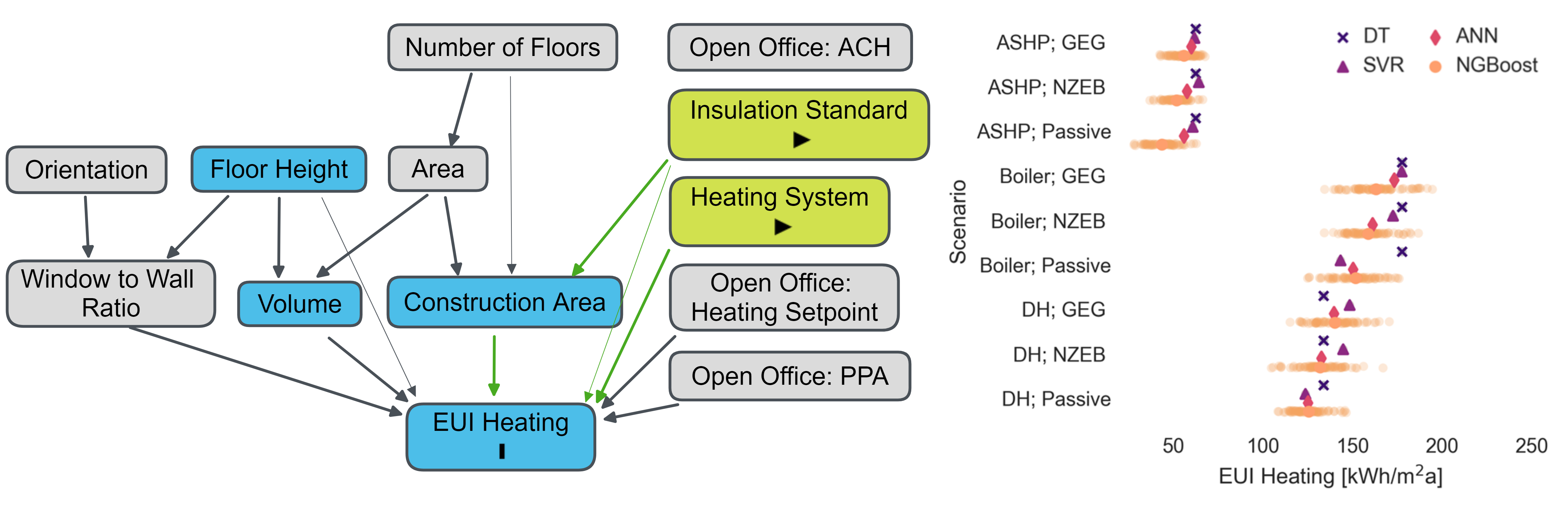
Figure 5: Minimal sufficient adjustment set based on the case: With Floor Height, Volume and Construction Area as extra inputs, the model generates unbiased estimation with sufficient information from the dataset.

Finally, it is essential to point out that DAGs and the minimal sufficient adjustment set solely provide identification information to ensure unbiased estimation, rather than addressing estimation performance. In engineering contexts, this data-driven process needs to relate to domain knowledge and thus be given context by the task-specific scenario for further analysis.

4 Discussion

We utilize a fallout case to demonstrate an easily identifiable error when using data-driven models. However, identifying such errors could be much more challenging for designers in many cases, potentially leading to a distrust in data-driven methods.

While these easily identifiable errors primarily appear in data-driven methods, similar risks of biased information exist when using first-principles simulations. First-principles simulations, extensively developed by numerous engineers and experts, carry their own biases (Rakitta and Wernery, 2021; Klotz, 2011; Zalewski et al., 2017). The difference is that these biases are often hidden or subtle due to the established and extensively developed nature of these simulations. Cognitive biases (Minsky, 1991), which refer to systematic errors in thinking that affect people’s decisions and judgments, can also cause such fallout situations. An example of a cognitive bias relevant in this context is confirmation bias, where engineers might favor information (e.g., a familiar type of design pattern, system deployment, or validation method) that confirms their preexisting beliefs or hypotheses while ignoring or downplaying contrary evidence. This bias leads to a skewed acquisition or utilization of personal domain knowledge. Considering the potential for cognitive biases, simulation results also bear fallout risks and often lack an appropriate adjustment mechanism. In this context, causal analysis serves as a useful tool for identifying potential biases in prior data, thus building a bridge that links and reinforces domain knowledge with data-driven methods. We argue that data-driven methods and first-principles simulations are not inherently conflicting. Rather, combining them may offer a practical solution to manage and mitigate the risk of biased outcomes.

While managing cognitive biases is crucial, another significant aspect to consider is the process of feature selection. In the context of causal analysis, it may seem that the more features (input variables) involved in the modeling process, the more comprehensive the causal skeleton should be. Simply feeding more features into the modeling process doesn’t necessarily contribute to the accuracy improvement. We perceive this as a trade-off between precision and accuracy in describing the case:

• More detailed features formalize a good representation of the target case, reducing uncertainty with a more accurate description, but also raise the risk of biased variation analysis.

• Using fewer detailed features certainly reduces the risk of biased result analysis; however, a too simple feature representation might overlook important factors that could affect the result and lead to incorrect conclusions.

5 Conclusion

The evolution of engineering analysis methodologies has fostered synergetic interaction among data, domain knowledge, simulations, and data-driven methods. Our case study highlights the potential pitfalls of relying solely on data-driven methods without incorporating causal analysis. We proved that it is critical to examine causal relationships when performing a data-driven analysis to avoid misleading results. Consequently, we advocate for more attention and involvement in causal inference analysis in the engineering community. Moreover, we believe that extracting invariant and transferable information from data is crucial in bridging the gap between domain knowledge, simulations, and data-driven methods in engineering and transcending individual capabilities’ limitations.

6 Acknowledgement

We gratefully acknowledge the German Research Foundation (DFG) support for funding the project under grant GE 1652/3-2 in the Researcher Unit FOR 2363 and under grant GE 1652/4-1 as a Heisenberg professorship.

7 Appendix

7.1 Mechanism Introduction of Machine Learning Methods

Tree-based models seek to identify optimal split points in the data to enhance prediction accuracy. The term "tree" refers to a decision tree, which forms the foundation of tree-based models. The decision tree algorithm identifies which data feature to split on and when to cease splitting based on information gain criteria (i.e., minimizing entropy in data split). While straightforward to interpret, decision trees are generally weak predictors. Enhanced ensemble methods such as bagging, random forest, boosting (Dietterich, 2000), and gradient boosting (Natekin and Knoll, 2013) have been adapted to improve performance but lead to less interpretable behavior.

Kernel machines utilize a linear classifier to address non-linear problems by defining a separating hyperplane to fit in data and make predictions. A kernel corresponds to a dot product in a typically high-dimensional feature space (Hofmann et al., 2008). In this space, estimation methods are linear, and all formulations are made in terms of kernel evaluations, thereby avoiding explicit computation in the high-dimensional feature space.

Neural networks comprise input, hidden, and output layers, where each layer is a group of neurons, loosely modeling the neurons in a biological brain. The connections between neurons (also called nodes) carry associated weights/biases. The data is fed into the network and passes through all neurons with activation functions (which add non-linearity to the output) in the forward propagation to produce output. The backpropagation mechanism (LeCun et al., 1988) updates neuron weights/biases according to the difference between prediction and output (loss function evaluation).

7.2 Modeling Configuration for Generating Training Data

The test case is a mixed-usage 4-floor building named Building.Lab on a tech campus in Regensburg, Germany (Chen et al., 2022b). The function of this 1,956 m² building is office and seminar use as well as housing, which consists of four above-ground stories and one underground level with a concrete skeleton structure. For supporting decision-making in energy-efficient building design, we developed a parametric model of an office building in a generic H-shape that covers a wide configuration variety of building components and zones. We varied this model to generate a representative training dataset for well-generalizing models on the target scenarios covering the design space characteristics of the case and similar buildings for performance evaluation. An illustration of the data generation process is given in Figure 6.

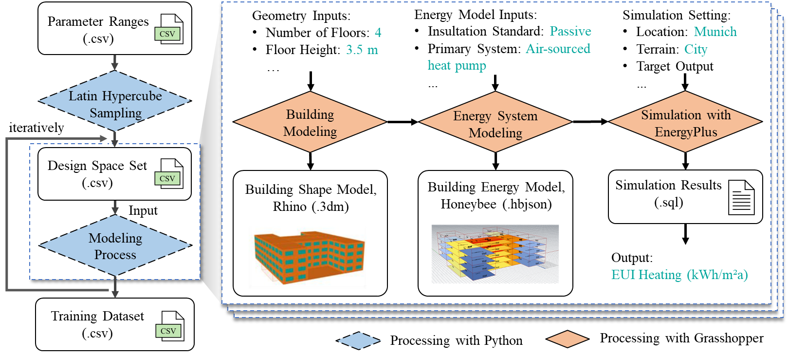
Figure 6: Automatic data generation process with parametric modeling: a generic H-shape office building. The parameter ranges are determined with the consideration of covering the test case scenario and densely sampled with variations. Each sample is fed iteratively into the energy simulation pipeline composited by Grasshopper, Python, and intermediate models. 918 samples were generated as the training dataset.

For the variation of building insulation standards, we simulated three component thermal characteristic sets based on real-world building energy standards and, from low to high: 2020 German Energy Act for Buildings (GEG), Net Zero Energy Building (NZEB), and Passive House. The standards have different requirements for components’ thermal conductivity (U-values), as presented in Table 5.

Table 5: Different insulation standard requirements for building component thermal characteristics [W/m²·K]

Insulation standard of U-Values in building components	Base: GEG (2020 German Energy Act for Buildings)	Medium: NZEB (Net Zero Energy Building)	High: Passive House
Base plate	0.2625	0.206	0.15
Roof	0.15	0.135	0.12
Exterior wall, bearing, above ground	0.21	0.18	0.15
Exterior wall, bearing, under ground	0.2625	0.206	0.15
Window	0.975	0.888	0.8

As for heating systems, three typical building energy systems are simulated: boiler, air-source heat pump (ASHP), and district heating (DH). All systems have been modeled with convective hot water baseboards as their secondary energy system. The hot water loop temperature was 50°C for the air-sourced heat pump system variant and 80°C for the boiler and district heating system variants. The piping system was modeled as adiabatic. The heating setpoint scales a typical office hour schedule to a new target setpoint. During off-work hours (starting from 6 pm), only 75% of the setpoint is set. Starting at 6 am, setpoints are increased hourly to 85%, 95%, and 100%. The minimum heating temperature is set to 21°C as we referred to the national standard DIN EN 16798-1 (Beu, ), and we intend to find sustainable and high-performing solutions (all options to be inside category I with PPD<6%). As the comfort temperature is 22°C ± 2K for environments below 16°C, we chose 21-24°C. In this simulation model, no cooling system and mechanical ventilation were modeled. The zone ventilation was only set by the air change rate per hour based on exterior air volume demands set from DIN EN 16798-1.

To validate the simulation result, we sampled the generated data (Training data) by different insulation standards and heating systems, as presented in Table 6 and Table 7, respectively.

Table 6: Energy Usage Intensity (EUI) Heating distribution, sampled by heating system choice

Energy Usage Intensity (EUI) Heating [kWh/m2a]	All		ASHP		Boiler		DH
	mean	std	mean	std	mean	std	mean	std
	84.6	50.1	45.4	13.5	143.0	44.6	106.3	31.6

Table 7: Energy Usage Intensity (EUI) Heating distribution, sampled by insulation standard

Energy Usage Intensity (EUI) Heating [kWh/m2a]	All		GEG		NZEB		Passive
	mean	std	mean	std	mean	std	mean	std
	84.6	50.1	90.8	56.5	85.1	49.0	78.0	45.1

7.3 Training Process and Result Validation

During the model training process, a hyperparameter grid-search strategy with 5-fold cross-validation (Refaeilzadeh et al., 2009) is applied for fitting data scheme changes in each scenario for all ML models. From an intuitive understanding, it means the same model with all hyperparameter setting combinations are cross evaluated within the 80/20 split training data, to compare and ensure the models’ best performance for test case validation. The results analysis by three evaluation metrics in all scenarios is presented in Table 8.

Table 8: 5-fold cross-validation performance result comparison of different models, all scenarios.

		Decision Tree	SVR	ANN	NGBoost
Scenario I	NRMSE	8.22	7.85	4.04	4.51
	SMAPE	0.15	0.14	0.10	0.09
	R2	0.86	0.87	0.96	0.95
Scenario II	NRMSE	9.70	7.81	5.35	7.48
	SMAPE	0.18	0.14	0.10	0.14
	R2	0.81	0.87	0.94	0.88
Validation	NRMSE	9.58	6.81	4.43	7.05
	SMAPE	0.18	0.11	0.09	0.14
	R2	0.81	0.90	0.96	0.90

References

- Bertolini et al. [2021] Massimo Bertolini, Davide Mezzogori, Mattia Neroni, and Francesco Zammori. Machine learning for industrial applications: A comprehensive literature review. Expert Systems with Applications, 175:114820, 2021.
- LeCun et al. [2015] Yann LeCun, Yoshua Bengio, and Geoffrey Hinton. Deep learning. nature, 521(7553):436–444, 2015.
- Raschka et al. [2020] Sebastian Raschka, Joshua Patterson, and Corey Nolet. Machine learning in python: Main developments and technology trends in data science, machine learning, and artificial intelligence. Information, 11(4):193, 2020.
- Dimiduk et al. [2018] Dennis M Dimiduk, Elizabeth A Holm, and Stephen R Niezgoda. Perspectives on the impact of machine learning, deep learning, and artificial intelligence on materials, processes, and structures engineering. Integrating Materials and Manufacturing Innovation, 7:157–172, 2018.
- Marcher et al. [2020] Carmen Marcher, Andrea Giusti, and Dominik T Matt. Decision support in building construction: A systematic review of methods and application areas. Buildings, 10(10):170, 2020.
- Seyedzadeh et al. [2018] Saleh Seyedzadeh, Farzad Pour Rahimian, Ivan Glesk, and Marc Roper. Machine learning for estimation of building energy consumption and performance: a review. Visualization in Engineering, 6:1–20, 2018.
- Schölkopf [2022] Bernhard Schölkopf. Causality for machine learning. In Probabilistic and Causal Inference: The Works of Judea Pearl, pages 765–804. 2022.
- Aldrich [1995] John Aldrich. Correlations genuine and spurious in pearson and yule. Statistical science, pages 364–376, 1995.
- Pearl and Mackenzie [2018] Judea Pearl and Dana Mackenzie. The book of why: the new science of cause and effect. Basic books, 2018.
- Chakraborty and Elzarka [2019] Debaditya Chakraborty and Hazem Elzarka. Advanced machine learning techniques for building performance simulation: a comparative analysis. Journal of Building Performance Simulation, 12(2):193–207, 2019.
- Hegde and Rokseth [2020] Jeevith Hegde and Børge Rokseth. Applications of machine learning methods for engineering risk assessment–a review. Safety science, 122:104492, 2020.
- Schölkopf et al. [2021] Bernhard Schölkopf, Francesco Locatello, Stefan Bauer, Nan Rosemary Ke, Nal Kalchbrenner, Anirudh Goyal, and Yoshua Bengio. Toward causal representation learning. Proceedings of the IEEE, 109(5):612–634, 2021.
- Chen et al. [2022a] Xia Chen, Jimmy Abualdenien, Manav Mahan Singh, André Borrmann, and Philipp Geyer. Introducing causal inference in the energy-efficient building design process. Energy and Buildings, 277:112583, 2022a.
- Spirtes [2010] Peter Spirtes. Introduction to causal inference. Journal of Machine Learning Research, 11(5), 2010.
- Pearl [2009] Judea Pearl. Causal inference in statistics: An overview. 2009.
- Spirtes et al. [2000] Peter Spirtes, Clark N Glymour, and Richard Scheines. Causation, prediction, and search. MIT press, 2000.
- Peters et al. [2017] Jonas Peters, Dominik Janzing, and Bernhard Schölkopf. Elements of causal inference: foundations and learning algorithms. The MIT Press, 2017.
- Kalisch and Bühlmann [2014] Markus Kalisch and Peter Bühlmann. Causal structure learning and inference: a selective review. Quality Technology & Quantitative Management, 11(1):3–21, 2014.
- DeVore and Temlyakov [1996] Ronald A DeVore and Vladimir N Temlyakov. Some remarks on greedy algorithms. Advances in computational Mathematics, 5:173–187, 1996.
- Chickering [2002a] David Maxwell Chickering. Learning equivalence classes of bayesian-network structures. The Journal of Machine Learning Research, 2:445–498, 2002a.
- Chickering [2002b] David Maxwell Chickering. Optimal structure identification with greedy search. Journal of machine learning research, 3(Nov):507–554, 2002b.
- Judea [2010] Pearl Judea. An introduction to causal inference. The International Journal of Biostatistics, 6(2):1–62, 2010.
- Pearl et al. [2000] Judea Pearl et al. Models, reasoning and inference. Cambridge, UK: CambridgeUniversityPress, 19(2):3, 2000.
- Guo et al. [2020] Ruocheng Guo, Lu Cheng, Jundong Li, P Richard Hahn, and Huan Liu. A survey of learning causality with data: Problems and methods. ACM Computing Surveys (CSUR), 53(4):1–37, 2020.
- Textor [2015] Johannes Textor. Drawing and analyzing causal dags with dagitty. arXiv preprint arXiv:1508.04633, 2015.
- Textor et al. [2016] Johannes Textor, Benito Van der Zander, Mark S Gilthorpe, Maciej Liśkiewicz, and George TH Ellison. Robust causal inference using directed acyclic graphs: the r package ‘dagitty’. International journal of epidemiology, 45(6):1887–1894, 2016.
- Singh et al. [2016] Amanpreet Singh, Narina Thakur, and Aakanksha Sharma. A review of supervised machine learning algorithms. In 2016 3rd international conference on computing for sustainable global development (INDIACom), pages 1310–1315. Ieee, 2016.
- Clark and Pregibon [2017] Linda A Clark and Daryl Pregibon. Tree-based models. In Statistical models in S, pages 377–419. Routledge, 2017.
- Hofmann et al. [2008] Thomas Hofmann, Bernhard Schölkopf, and Alexander J Smola. Kernel methods in machine learning. 2008.
- Chen and Geyer [2022] Xia Chen and Philipp Geyer. Machine assistance in energy-efficient building design: A predictive framework toward dynamic interaction with human decision-making under uncertainty. Applied Energy, 307:118240, 2022.
- Tian et al. [2018] Wei Tian, Yeonsook Heo, Pieter De Wilde, Zhanyong Li, Da Yan, Cheol Soo Park, Xiaohang Feng, and Godfried Augenbroe. A review of uncertainty analysis in building energy assessment. Renewable and Sustainable Energy Reviews, 93:285–301, 2018.
- Duan et al. [2020] Tony Duan, Avati Anand, Daisy Yi Ding, Khanh K Thai, Sanjay Basu, Andrew Ng, and Alejandro Schuler. Ngboost: Natural gradient boosting for probabilistic prediction. In International conference on machine learning, pages 2690–2700. PMLR, 2020.
- Chen et al. [2022b] X. Chen, U. Saluz, J. Staudt, M. Margesin, W. Lang, and P. Geyer. Integrated data-driven and knowledge-based performance evaluation for machine assistance in building design decision support. In Proceedings of the 29th EG-ICE International Workshop on Intelligent Computing in Engineering. EG-ICE, June 2022b. doi:10.7146/aul.455.c202. URL https://doi.org/10.7146/aul.455.c202.
- McNeel et al. [2022] Robert McNeel et al. Grasshopper-new in rhino 6, 2022.
- Ladybug Tools [2021] LLC Ladybug Tools. Ladybug tools. Computer software]. https://www. ladybug. tools, 2021.
- Chicco et al. [2021] Davide Chicco, Matthijs J Warrens, and Giuseppe Jurman. The coefficient of determination r-squared is more informative than smape, mae, mape, mse and rmse in regression analysis evaluation. PeerJ Computer Science, 7:e623, 2021.
- Balestriero et al. [2021] Randall Balestriero, Jerome Pesenti, and Yann LeCun. Learning in high dimension always amounts to extrapolation. arXiv preprint arXiv:2110.09485, 2021.
- Chen et al. [2022c] Xia Chen, Tong Guo, Martin Kriegel, and Philipp Geyer. A hybrid-model forecasting framework for reducing the building energy performance gap. Advanced Engineering Informatics, 52:101627, 2022c.
- Roman et al. [2020] Nadia D Roman, Facundo Bre, Victor D Fachinotti, and Roberto Lamberts. Application and characterization of metamodels based on artificial neural networks for building performance simulation: A systematic review. Energy and Buildings, 217:109972, 2020.
- Patil et al. [1981] Ramesh S Patil, Peter Szolovits, and William B Schwartz. Causal understanding of patient illness in medical diagnosis. In Computer-Assisted Medical Decision Making, pages 272–292. Springer, 1981.
- Greenland et al. [1999] Sander Greenland, Judea Pearl, and James M Robins. Causal diagrams for epidemiologic research. Epidemiology, pages 37–48, 1999.
- Shrier and Platt [2008] Ian Shrier and Robert W Platt. Reducing bias through directed acyclic graphs. BMC medical research methodology, 8:1–15, 2008.
- Rakitta and Wernery [2021] M Rakitta and J Wernery. Cognitive biases in building energy decisions. sustainability 2021, 13, 9960, 2021.
- Klotz [2011] Leidy Klotz. Cognitive biases in energy decisions during the planning, design, and construction of commercial buildings in the united states: an analytical framework and research needs. Energy Efficiency, 4:271–284, 2011.
- Zalewski et al. [2017] Andrzej Zalewski, Klara Borowa, and Andrzej Ratkowski. On cognitive biases in architecture decision making. In Software Architecture: 11th European Conference, ECSA 2017, Canterbury, UK, September 11-15, 2017, Proceedings 11, pages 123–137. Springer, 2017.
- Minsky [1991] Marvin L Minsky. Logical versus analogical or symbolic versus connectionist or neat versus scruffy. AI magazine, 12(2):34–34, 1991.
- Dietterich [2000] Thomas G Dietterich. Ensemble methods in machine learning. In International workshop on multiple classifier systems, pages 1–15. Springer, 2000.
- Natekin and Knoll [2013] Alexey Natekin and Alois Knoll. Gradient boosting machines, a tutorial. Frontiers in neurorobotics, 7:21, 2013.
- LeCun et al. [1988] Yann LeCun, D Touresky, G Hinton, and T Sejnowski. A theoretical framework for back-propagation. In Proceedings of the 1988 connectionist models summer school, volume 1, pages 21–28. San Mateo, CA, USA, 1988.
- [50] DIN EN 16798-1:2022-03, energetische bewertung von gebäuden_- lüftung von gebäuden_- teil_1: Eingangsparameter für das innenraumklima zur auslegung und bewertung der energieeffizienz von gebäuden bezüglich raumluftqualität, temperatur, licht und akustik_- modul m1-6; deutsche fassung EN_16798-1:2019. URL https://doi.org/10.31030/3327351.
- Refaeilzadeh et al. [2009] Payam Refaeilzadeh, Lei Tang, and Huan Liu. Cross-validation. Encyclopedia of database systems, pages 532–538, 2009.