Off-shell selfenergy for 1-D Fermi liquids

Abstract

The selfenergy in Born approximation including exchange of interacting one-dimensional systems is expressed in terms of a single integral about the potential which allows a fast and precise calculation for any potential analytically. The imaginary part of the self energy as damping of single-particle excitations shows a rich structure of different areas limited by single-particle and collective excitation lines. The corresponding spectral function reveals a pseudogap, a splitting of excitation into holons and antiholons as well as bound states.

I Introduction

Interacting Fermi systems in one dimension appear in many physical situations. Among them let us mention only quantum wires in carbon nanotubes Saito98 ; Bockrath99 ; Ishii03 ; Shiraishi03 or edge states in quantum hall liquid Milliken96 ; Mandal01 ; Chang03 , semiconducting nanowires Schafer08 ; Huang01 , cold atomic gases Monien98 ; Recati03 ; Moritz05 , conducting molecules Nitzan03 or even crystalline ion beams in storage rings SSH01 ; SSBH02 .

Though exact solutions are known for Luttinger L63 ; LP74 ; ES07 , Tomonaga DL74 , and Gaudin-Yang models Ram17 ; Pan22 of contact interaction by the Bethe ansatz EFGKK10 ; GBML13 the interacting Fermi system in quantum wires are still a theoretical challenge. Among these methods bosonization techniques in Lu77 ; Solyom79 and out of GGM10 equilibrium are employed which are based on the similar behaviour of long-distance correlations of Fermi and Bose systems H81a . The underlying model is the continuum limit which has been discussed with the help of correlation functions Emery79 . Already the width dependence GADMP22 of quantum wires escapes exact solutions and perturbation methods have been used to investigate analytically and numerically the ground-state properties LD11 ; LG16 ; Loos13 . The question is how relevant are results from perturbation theory for such strongly correlated one-dimensional Fermi system. In MVBP18 it was shown that the Random Phase Approximation becomes exact in the high-density limit for one-dimensional systems.

This peculiar feature of a perturbation series to become exact is due to the fact that in one dimensions the ratio of kinetic to interaction energy is proportional to the density. Therefore the weak coupling corresponds to the high-density regime and the strong coupling regime to low densities GPS08 . Contrary to three dimensions one can therefore describe the high-density limit by a weak-coupling theory, i.e. perturbation theory. Though we cannot expect quantitative correct results by Born approximation as first-order perturbation theory of collisional damping, we might get insight into high-density correlations. Conventionally, perturbation theory is considered to fail in one dimensions due to divergences at the Fermi energy. Recently this was cured by a Padé approximation and an extended quasiparticle picture does work indeed M23 .

The selfenergy represents the fundamental quantity to study single-particle correlation and excitation effects. This is best described within the Green function technique, for an overview see V94 ; G04 ; GV08 ; M17b . Green functions allow to investigate interacting models beyond exactly solvable cases and in various approximations T67 ; VMKA08 . The transition between Tomonaga-Luttinger and Fermi liquids has been studiedSch77 ; Yo01 and the resulting non-Fermi liquid behaviour has been numerically shown for Tomonaga Luttinger processes in Sch95 . For contact interaction the exact Green function has been known for a long time T67 where even the finite-size effect of the potential has been discussed. The exact impurity Green function for contact interaction was presented in Ga15 . The elastic two-particle collision in one dimension can only lead to an exchange of momenta of the two particles due to energy-momentum conservation which means that the on-shell selfenergy vanishes.

In contrast, the off-shell selfenergy can provide an interesting insight into the physics of strongly correlated one-dimensional system. Therefore we will provide analytical expressions for the off-shell selfenergy for electron-electron interactions in Born approximation including exchange. Due to numerous analytic reductions we present a scheme with a single integral over the potential which can be applied in a variety of situations.

The outline of the paper is as follows. Next we present the analytical result of the imaginary part of selfenergy in Born approximation including exchange. The nontrivial integration is shifted to the appendix and the particle and hole contributions to the selfenergy are discussed. Multiple ranges appear in the plot of momentum versus off-shell energy. They can be understood as originating from collective and single-particle excitations completely nested since in one dimensions the Fermi surface consists only of two points. The real part of the selfenergy as a Hilbert transform is presented in chapter III where the details are again moved to the appendix. Both the imaginary and real part of the selfenergy are expressed by a single integral over any chosen potential which allows a precise and fast calculation with a wide range of applications. Taking additionally the Hartree-Fock selfenergy into account, in chapter IV the spectral function is discussed up to quadratic orders in the potential or Bruckner coupling parameter. Chapter V summarizes and gives some conclusions.

II Self energy in Born approximation

The real part of the selfenergy is the Hilbert transform

$$\sigma(k,\omega)={\rm Re}\,\sigma^{R}(k,\omega)=\int{d\bar{\omega}\over 2\pi}{\gamma(k,\bar{\omega})\over\omega-\bar{\omega}}$$ (1)

of the selfenergy spectral function or imaginary part

$$\gamma=\sigma^{>}+\sigma^{<}=i(\sigma^{R}-\sigma^{A})=-2{\rm Im}\,\sigma^{R}.$$ (2)

Both specifying the retarded selfenergy

$$\sigma^{R}(k,\omega)=\sigma(k,\omega)-\frac{i}{2}\gamma(k,\omega)=\int{d\bar{\omega}\over 2\pi}{\gamma(\bar{\omega})\over\omega-\bar{\omega}+i\eta}.$$ (3)

Here the electron momentum is $k$ and the off-shell energy is denoted by $\omega$. From the collision integral

$$I=n_{k}\sigma^{>}-(1-n_{k})\sigma^{<}$$ (4)

one sees that $\sigma^{>}$ describes the contribution of damping due to particles characterized by the Fermi distribution $n_{k}$ and $\sigma^{<}$ the contribution to the damping due to holes $1-n_{k}$.

II.1 Hole contribution to the damping

The selfenergy in Born approximation reads

$$\sigma^{<}(k,\omega) = \sum\limits_{qp}2\pi\delta(\omega\!+\!\epsilon_{p}\!-\!\epsilon_{p\!-\!q}\!-\!\epsilon_{k\!+\!q})n_{p\!-\!q}n_{k\!+\!q}(1\!-\!n_{p})$$ (5)

$$\times V_{q}\left[sV_{q}-V_{p-k-q}\right]$$

where the spin degeneracy $s$ does only apply to the direct and not to the exchange terms. The $\sigma^{>}$ selfenergy is obtained by interchanging the distribution or occupation factors $n\leftrightarrow 1-n$. In the following we understand all energies, $\omega,\gamma,\sigma$ etc, in units of Fermi energy $\epsilon_{f}$ and the momenta $k$ in units of Fermi momentum given by the free-particle density $n_{f}$ as $k_{F}=n_{f}\hbar\pi/s$. The interaction strength we express in terms of $a_{B}$, the Bohr-radius-equivalent

$$V_{q}={\hbar^{2}\over ma_{B}}v_{q}$$ (6)

which allows to discuss charged and neutral impurities on the same footing. The Brueckner parameter $r_{s}$ is the ratio of inter-particle distance $d=1/ns$ to this length $r_{s}=d/a_{B}$.

The $\delta$-function in (5) is carried out which means to replace

$$p=q+k-{\Omega\over 2q},\quad\Omega=\omega-k^{2}$$ (7)

and providing an additional $m/|q|$ prefactor. Together with the potential, it becomes

$$\delta(\omega\!+\!\epsilon_{p}\!-\!\epsilon_{p\!-\!q}\!-\!\epsilon_{k\!+\!q})V_{q}\left[sV_{q}-V_{p-k-q}\right]$$

$$={\hbar^{4}\over ma_{B}^{2}}\delta\left(p-q-k+{\Omega\over 2q}\right){v_{q}\over|q|}\left(sv_{q}-v_{\Omega\over 2q}\right).$$ (8)

The implication of the occupation factors on the range of $q$-integration turns out to be quite non-trivial and are discussed in appendix A. We abbreviate

$$a^{2}={|\Omega|\over 2}={k^{2}-\omega\over 2}>0$$ (9)

in the following since it is convenient when we will calculate the Hilbert transform for the real part of the selfenergy in the next chapter.

The result for (5) reads

$$0<k<1$$

$$\quad\sigma^{<}=\Phi(1-k)-\Phi\left({a^{2}\over 1-k}\right) {\rm for} \,0\!<\!a\!<\!1\!-\!k \leftrightarrow\, 2-(k-2)^{2}<\omega<k^{2} {\rm area:}\,1,2,3$$

$$\quad\sigma^{<}=\Phi(q_{2})-\Phi(q_{1}) {\rm for} \,0<a<{1-k\over 2} \leftrightarrow\, {(k+1)^{2}\over 2}-1<\omega<k^{2} {\rm area:}\,1$$

$$\quad\sigma^{<}=\Phi(1+k)-\Phi\left({a^{2}\over 1+k}\right) {\rm for} \,0\!<\!a\!<\!1\!+\!k \leftrightarrow\, 2-(k+2)^{2}<\omega<k^{2} {\rm area:}\,1,3,5$$

$$\quad\sigma^{<}=\Phi(\bar{q}_{2})-\Phi(\bar{q}_{1}) {\rm for} \,0<a<{1+k\over 2} \leftrightarrow\, {(k-1)^{2}\over 2}-1<\omega<k^{2} {\rm area:}\,1,2,3,4,5$$

$$1<k<3$$

$$\quad\sigma^{<}=\Phi\left({a^{2}\over-1+k}\right)-\Phi(k-1) {\rm for} \,\sqrt{-2(1-k)}\!<\!a\!<\!\sqrt{k^{2}-1} \leftrightarrow\, 2-k^{2}<\omega<(k-2)^{2} {\rm area:}\,6,7$$

$$\quad\sigma^{<}=\Phi(1+k)-\Phi\left({a^{2}\over 1+k}\right) {\rm for} \,\sqrt{k^{2}-1}\!<\!a\!<\!{1\!+\!k} \leftrightarrow\, 2-(k+2)^{2}<\omega<2-k^{2} {\rm area:}\,4,5$$

$$\quad\sigma^{<}=\Phi(\bar{q}_{2})-\Phi(\bar{q}_{1}) {\rm for} \,\sqrt{-2(1-k)}<a<{1+k\over 2} \leftrightarrow\, {(k-1)^{2}\over 2}-1<\omega<(k-2)^{2} {\rm area:}\,5,6$$

$$3<k$$

$$\quad\sigma^{<}=\Phi\left({a^{2}\over-1+k}\right)-\Phi(-1+k) {\rm for} \,1-k\!<\!a\!<\!\sqrt{k^{2}-1} \leftrightarrow\, 2-k^{2}<\omega<2-(k-2)^{2} {\rm area:}\,7$$

$$\quad\sigma^{<}=\Phi(1+k)-\Phi\left({a^{2}\over 1+k}\right) {\rm for} \,\sqrt{k^{2}-1}\!<\!a\!<\!1+k \leftrightarrow\, 2-(k+2)^{2}<\omega<2-k^{2} {\rm area:}\,4$$ (10)

with (41)

$$q_{1/2}={1-k\over 2}\pm\sqrt{{(1-k)^{2}\over 4}-a^{2}}.$$ (11)

and $\bar{q}_{1/2}$ are (11) with $k\to-k$. This expression (10) is solely given in terms of a single integral over the potential

$$\Phi(q)={s^{4}r_{s}^{2}\over\pi^{3}}\int\limits^{q}d\bar{q}{v_{\bar{q}}\over|\bar{q}|}\left(sv_{q}-v_{\Omega\over 2q}\right)$$ (12)

which can be calculated analytically (44) for contact potential and a model potential we will use

$$v_{q}={1\over\sqrt{q^{2}+\kappa^{2}}}.$$ (13)

Here the finite-size parameter $\kappa$ describes the width of the wire or alternatively the screening of Coulomb potential $v_{q}\sim 1/q$.

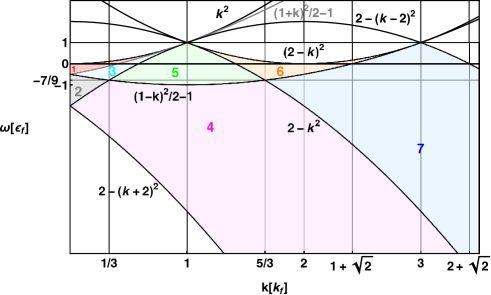
Figure 1: The 7 different areas for the selfenergy $\sigma^{<}$ according to (10).

Seven different areas in frequency $\omega$ appear and are plotted in figure 1. The border curves between these areas have a physical meaning. The part $\sigma^{<}$ describes the damping due to holes and lays below the on-shell $\omega=k^{2}$. Since the one-dimensional system is maximally nested we do have all borders also with $k\to k\pm 2$. i.e. also below the shell $(k-2)^{2}$.

The borders $(1\pm k)^{2}/2-1$ can be understood as arising from the collective behaviour. Since the Fermi surface shrinks at T = 0 to two points the single-particle excitation turn into collective one SDC19 . The lowest-order polarization in random phase approximation reads

$$\Pi_{0}(q,\omega)={ms\over\pi p_{f}\hbar}\int{dp}{n_{p+\frac{q}{2}}-n_{p-\frac{q}{2}}\over(p+\frac{q}{2})^{2}-(p-\frac{q}{2})^{2}-\omega-i0}$$ (14)

which becomes for zero temperature MVBP18 ; VBMP19

$${\rm Im}\Pi_{0} = -{ms\over 2\hbar p_{f}q}\Theta(\omega-|\omega_{-}|)\Theta(|\omega_{+}|-\omega),$$

$${\rm Re}\Pi_{0} = {ms\over 2\pi\hbar p_{f}q}\ln{\left|{\omega^{2}-\omega_{-}^{2}\over\omega^{2}-\omega_{+}^{2}}\right|}$$ (15)

with $\omega_{\pm}={q}(q\pm 2)$ in units of Fermi energy. This gives the limiting line where collective excitations occur. Subtracting the Fermi energy and considering the reduced mass due to two-particle scattering translates into $(1\pm q)^{2}/2-1$ lines of figure 1. These borders indicates the divergence of polarization known as Kohn anomaly and which are the reason for Peierls instability.

The second class of lines are $2-k^{2}$, or nested as $2-(k\pm 2)^{2}$, arising from single particle excitation Pan22 due to off-shell scattering. For explanation we consider a simple model in figure 2 similar to G04 . The excitation of a particle with momentum $k$ out of the Fermi sea $\omega_{k}(q)=\epsilon_{k+q}-\epsilon_{k}$ due to scattering with momentum $q$ arises for possible particle momenta $k\in(k_{f}-q,k_{f})$ for $k<2k_{f}$ and $k\in(-k_{f},k_{f})$ for $k>2k_{f}$. Averaging this excitation $w_{k}(q)$ about the possible interval $k$ and choosing as fluctuation the maximum and minimum possible excitation in this interval we obtain in units of Fermi energy

$$\omega(q)=\left\{\begin{array}[]{cc}2q\pm 2q^{2};&q<2\cr q^{2}\pm 4q;&q>2\end{array}\right.$$ (18)

which second case yields after subtracting from the two Fermion threshold the curves $2-(k\pm 2)^{2}$ in figure 1.

Figure 2: The scheme of possible single-particle excitation due to scattering out of Fermi sea.

For contact interaction we plot in figures 3 the selfenergy $\sigma^{<}$ for different momenta cuts according to figure 1 covering the crossing of various areas by frequency. One sees a continuous but non-differentiable behaviour.

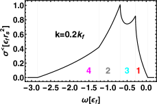
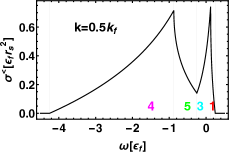
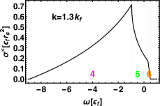
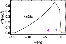
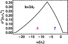
Figure 3: The selfenergy $\sigma^{<}$ of contact interaction for different momentum cuts and regions numbers of figure 1.

II.2 Particle contribution to the damping

The second part of the damping (2) due to particles reads

$$\sigma^{>}(k,\omega) = \sum\limits_{qp}V_{q}\left[sV_{q}-V_{p-k-q}\right]2\pi\delta(\omega\!+\!\epsilon_{p}\!-\!\epsilon_{p\!-\!q}\!-\!\epsilon_{k\!+\!q})$$ (19)

$$\times(1\!-\!n_{p\!-\!q})(1\!-\!n_{k\!+\!q})n_{p}$$

which integration is presented in appendix B. We have to distinguish two cases.

In the first case, $\Omega=\omega-k^{2}<0$, we obtain

$$1<k<3$$

$$\quad\sigma^{>}=\Phi(-1+k)-\Phi\left({a^{2}\over-1+k}\right) {\rm for} \,0\!<\!a\!<\!k-1 \leftrightarrow\, 2-(k-2)^{2}<\omega<k^{2} {\rm area:}\,4,5$$

$$\quad\sigma^{>}=\Phi(\bar{q}_{1})-\Phi(\bar{q}_{2}) {\rm for} \,0\!<\!a\!<\!{(k\!-\!1)\over 2} \leftrightarrow\, {(k+1)^{2}\over 2}-1<\omega<k^{2} {\rm area:}\,5,7$$

$$3<k$$

$$\quad\sigma^{>}=\Phi(\bar{q}_{1})-\Phi(\bar{q}_{2}) {\rm for} \,0\!<\!a\!<\!{(k\!-\!1)\over 2} \leftrightarrow\, {(k+1)^{2}\over 2}-1<\omega<k^{2} {\rm area:}\,4,5,7$$

$$\quad\sigma^{>}=\Phi(-1+k)-\Phi({a^{2}\over-1+k}) {\rm for} \,0\!<\!a\!<\!\sqrt{2(k-1)} \leftrightarrow\, (k-2)^{2}<\omega<k^{2} {\rm area:}\,4,5$$

$$\quad\sigma^{>}=\Phi(\bar{q}_{4})-\Phi(\bar{q}_{3}) {\rm for} \,\sqrt{2(k-1)}\!<\!a\!<\!{1+k\over 2} \leftrightarrow\, {(k-1)^{2}\over 2}-1<\omega<(k-2)^{2} {\rm area:}\,6,7$$ (20)

with (12),

$$q_{3/4}={-1-k\over 2}\pm\sqrt{{(1+k)^{2}\over 4}-a^{2}},$$ (21)

and $\bar{q}_{3/4}$ are (21) with $k\to-k$. This case contributes to the ranges $4-7$ plotted in figure 4.

In the second case $\Omega=\omega-k^{2}>0$ we obtain different areas and arguments

$$0<k<1$$

$$\quad\sigma^{>}=\Phi\left({a^{2}\over 1+k}\right)-\Phi(k+1) {\rm for} \,\sqrt{1-k^{2}}\!<\!a\!<\!\sqrt{2(1+k)} \leftrightarrow\, 2-k^{2}<\omega<(k+2)^{2} {\rm area:}\,4$$

$$\quad\sigma^{>}=\Phi\left({a^{2}\over 1-k}\right)-\Phi(1-k) {\rm for} \,\sqrt{1-k^{2}}\!<\!a\!<\!\sqrt{2(1-k)} \leftrightarrow\, 2-k^{2}<\omega<(k-2)^{2} {\rm area:}\,1$$

$$\quad\sigma^{>}=\Phi\left(\bar{q}_{7}\right)-\Phi(q_{8}) {\rm for} \,\sqrt{2(1-k)}\!<\!a\!<\!\infty \leftrightarrow\, (k-2)^{2}<\omega<\infty {\rm area:}\,2,3,4$$

$$\quad\sigma^{>}=\Phi\left(q_{7}\right)-\Phi(\bar{q}_{8}) {\rm for} \,\sqrt{2(1+k)}\!<\!a\!<\!\infty \leftrightarrow\, (k+2)^{2}<\omega<\infty {\rm area:}\,3$$

$$1<k$$

$$\quad\sigma^{>}=\Phi\left({a^{2}\over 1+k}\right)-\Phi(k+1) {\rm for} \,0<a<\sqrt{2(1\!+\!k)} \leftrightarrow\, k^{2}<\omega<(k+2)^{2} {\rm area:}\,4$$

$$\quad\sigma^{>}=\Phi\left(\bar{q}_{7}\right)-\Phi(q_{8}) {\rm for} \,0<a<\infty \leftrightarrow\, k^{2}<\omega<\infty {\rm area:}\,2,3,4$$

$$\quad\sigma^{>}=\Phi\left(q_{7}\right)-\Phi(\bar{q}_{8}) {\rm for} \,\sqrt{2(1+k)}\!<\!a\!<\!\infty \leftrightarrow\, {(k+1)^{2}\over 2}-1<\omega<k^{2} {\rm area:}\,3$$ (22)

with (12), $a^{2}={|\Omega|/2}={(\omega-k^{2})/2}$,

$$q_{7/8}={\pm 1-k\over 2}+\sqrt{{(1\mp k)^{2}\over 4}+a^{2}},$$ (23)

and $\bar{q}_{7/8}$ are (23) with $k\to-k$. This case contributes to the ranges $1-4$ plotted in figure 4 which summarizes the different areas of (20) and (22). The occurring border lines are the same as in figure 1 explained there.

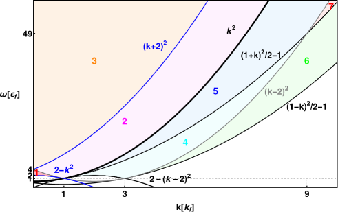
Figure 4: The 7 different areas for the selfenergy $\sigma^{>}$ according to (20) and (22).

In figures 5 the selfenergy $\sigma^{>}$ is presented for different momentum cuts covering the crossing of various areas by frequency in figure 4. One observes again a continuous but non-differentiable behaviour.

The figures 4 and 1 together gives the complete ranges of the imaginary part of the selfenergy. We like to point out that the Eq.s (10), (20) and (22) allow to calculate analytically this imaginary part for any interaction with the help of a single integral (12) which provides a fast and precise calculation.

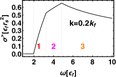
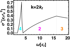
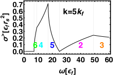
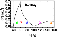
Figure 5: The selfenergy $\sigma^{>}$ of contact interaction for different momentum cuts of figure 4.

The finite-size potential (13) with (44) can be used as well and presented in figure 6. One sees exactly the same borderlines of areas as discussed above but different quantitative values dependent on the width parameter $\kappa$. For smaller $\kappa$ we approach the Coulomb potential and one sees that the peaks become enhanced.

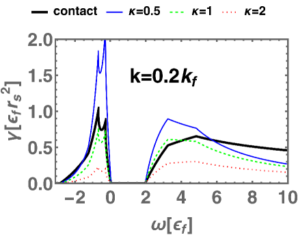
Figure 6: The imaginary part of selfenergy for contact interaction and three values of finite size potential (13).

III Real part of selfenergy

The Hilbert transform (1) we will perform in the appendix C and obtain with the help of a single integral about arbitrary potentials

$$\phi(x)={s^{5}r_{s}^{2}\over 2\pi^{4}}\int\limits^{x}{dx\over{\omega-k^{2}\over 2}+x}\left(sv_{q}-v_{x\over q}\right)$$ (24)

with the abbreviations

$$\Theta_{ij} = \Psi^{0}_{ij}-\Psi_{ij}$$

$$\Psi_{ij} = \phi(ikq+jq-q^{2}),\quad\Psi^{0}_{ij}=\phi(ikq+jq)$$ (25)

finally

$$\sigma =\int\limits_{0}^{2}\!\!dq{v_{q}\over q}\left(\Theta_{+-}\!+\!\Theta_{--}\right)$$

$$+\int\limits_{2}^{\infty}\!\!dq{v_{q}\over q}\left(\Psi_{++}\!+\!\Psi_{-+}-\Psi_{+-}\!-\!\Psi_{--}\right)$$

$$\!+\!\left\{\!\begin{array}[]{cc}\!\int\limits_{k-1}^{k+1}\!dq{v_{q}\over q}\,\left(\Theta_{++}\!-\!\Theta_{+-}\right)&k\!>\!1\cr\int\limits_{0}^{k+1}\!\!dq{v_{q}\over q}\left(\Theta_{++}\!-\!\Theta_{+-}\right)\!+\!\!\int\limits_{0}^{1-k}\!\!dq{v_{q}\over q}\left(\Theta_{-+}\!-\!\Theta_{--}\right)&k\!<\!1\end{array}\right..$$ (28)

The real and imaginary parts of the selfenergy are plotted in figure (7). One sees that for $k>2k_{f}$ the damping vanishes in a range $\omega\approx 2$ which is accompanied with a gap as seen in figure 6. Further a splitting of two excitation lines for positive frequencies and one for negative frequencies appear. Which of them finally survive and describe a real excitation in the system is decided by the spectral function in the next chapter.

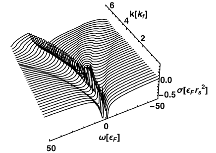
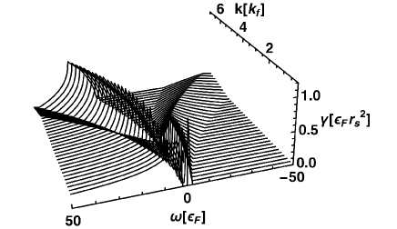
Figure 7: The real part $\sigma$ (above) and imaginary part $\gamma$ (below) of the selfenergy for contact interaction.

The finite size of a potential (13) is compared in figure 8 for different values of the screening parameter $\kappa$ with the contact interaction. For small $\kappa$ we approach Coulombic behaviour and see that the peak at the Fermi energy becomes enhanced.

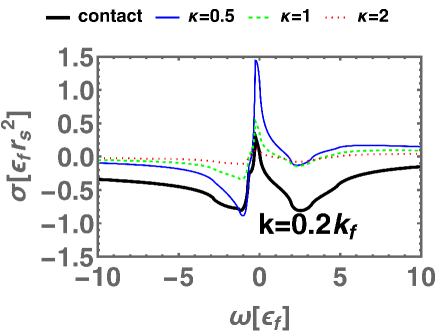
Figure 8: The real part of the selfenergy for contact interaction and three values of finite size potential (13) corresponding to the imaginary part in figure 6.

IV Spectral function

Now that we have the real and imaginary part of the selfenergy (2) we can calculate the spectral function as measure for the single-particle excitation in the system

$$a(\omega,k)={\gamma(\omega,k)\over[\omega-k^{2}-\sigma^{F}(k)-\sigma(\omega,k)]^{2}+{\gamma^{2}(\omega,k)\over 4}}.$$ (29)

The still missing part is the Hartree-Fock meanfield selfenergy as the part lower than Born in perturbation theory and it is necessary to include the meanfield in order to have all results systematically up to second order in the potential. The Hartree selfenergy proportional to the number of electrons $\sigma^{H}=nV_{0}$ is compensated by a neutralizing background. The Fock term as exchange meanfield term reads

$$\sigma^{F}(k) =-s\int\limits_{-\infty}^{\infty}{dq\over 2\pi\hbar}v_{q}n_{k-q}$$

$$=-{2s^{2}\over\pi^{2}}r_{s}\left\{\begin{array}[]{cc}1&{\rm contact}\cr&\cr\frac{2}{\pi^{2}}\ln\left|\frac{k-\sqrt{(k+1)^{2}+\text{kap}^{2}}+1}{-k+\sqrt{(1-k)^{2}+\text{kap}^{2}}+1}\right|&{\rm pot.}(\ref{pot})\end{array}\right.$$ (33)

which results for contact interaction $v_{q}=1$ and finite-size potential (13) respectively using the Bruckner or coupling parameter $r_{s}$.

In figures 9 and 10 we plot the spectral functions for a Bruckner parameter $r_{s}=0.5$ and $r_{s}=2$ respectively.

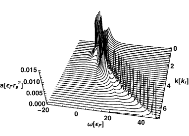
Figure 9: The spectral function (29) with coupling parameter $r_{s}=0.5$ for contact interaction (above) and for finite size (13) with $\kappa=0.5$ (below).

One recognizes the main excitation at $\omega=k^{2}$ line for large momenta. For contact interaction a splitting of the quasiparticle excitation pole appears at higher momenta which is absent in the finite-size or Coulombic potential. The characteristic feature of contact potential is more clearly visible for higher coupling in figure 10. A gap opens with the borders $\omega\approx\pm 2k$ (or in units $\hbar\omega\approx{p_{f}\over m}k$) which feature would be the exact borders for a Luttinger liquid V83 ; G04 . Here we do not have a Luttinger liquid but see similar features. The two peaks are related to holon and antiholon excitations, i.e. the excitation of a particle out of Fermi sea EFGKK10 , schematically illustrated in figure 2. The corresponding threshold singularities have been discussed in Ess10 . The deviation from the Luttinger liquid can be seen by the boundary of the gap in figure 7 which should be linear $\pm kv_{o}$ with the charge velocityVo93a ; MeS92 of $v_{0}=\sqrt{v_{f}^{2}+g^{2}}$. A spin-polarized system would show additionally a splitting of the peak in spin and charge velocities Vo93 ; G04 . Further we do have a finite width of the peaks of the spectral function in contrast to the Tomonaga-Luttinger model MeS92 . The appearance of the gap is also related to a pseudogap in the density of states Ta20 .

Up to the momentum of $k=2k_{f}$ there appear an excitation at negative frequencies which one interprets as bound states. Momenta above $2k_{f}$ correspond to nesting which means that this bound state is destroyed when nesting occurs. The occurrence of this bound state is puzzling since it appears in 3D only for higher-order approximations like the ladder summation. Since we consider the weak-coupling limit which is the high-density limit, we see probably here a precursor of bound states in the off-shell selfenergy.

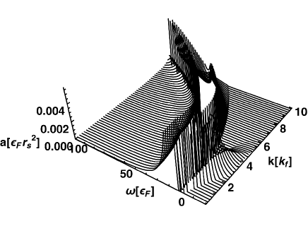
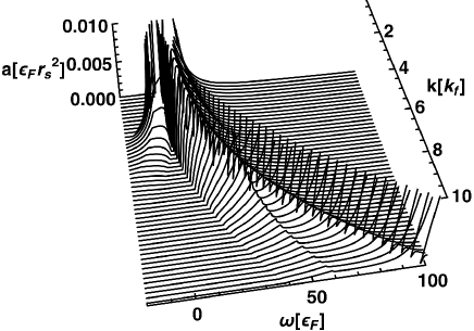
Figure 10: The spectral function (29) for contact interaction and a coupling parameter $r_{s}=2$ in different views.

V Summary and Conclusions

The Born selfenergy including exchange is expressed analytically with a remaining single integral for the imaginary part (12) and the real part (24) respectively. This allows to calculate the selfenergy precise and fast for any interaction potential. Therefore these expressions can be applied widely. The momentum-frequency range of different parts of the selfenergy turns out to be astonishing complex consisting of single-particle excitation and border lines of collective modes. This leads to a non-differentiable behaviour of the imaginary part of the selfenergy. The real part is worked down as well to a single integral which provides a fast scheme. Given the Born selfenergy together with the meanfield, the spectral function as measure for single-particle excitation is calculated for the illustrative examples of contact interaction and a finite-size potential. The opening of the Luttinger gap is seen with increasing momenta. Two excitation lines due to holon and antiholon excitations are observed. An excitation at negative frequencies is interpreted as precursor of bound states which vanishes for momenta exceeding $2p_{f}$ indicating nesting instead.

Appendix A q-integration of $\sigma<$

First we observe that it is only necessary to integrate half of the range $q>0$ in (5) since the area $q<0$ can be mapped to the $q>0$ expression if we set $k\to-k$. This can be seen in (5) since the $p$ integration allows to set $p\to-p$.

From occupation factors we get the conditions $\Omega=\omega-k^{2}$

$$n_{p-q}: -1+{\Omega\over 2q}<k<1+{\Omega\over 2q}$$ (34)

$$n_{k+q}: -1-q<k<1-q$$

$$1-n_{p}: k<-1-q+{\Omega\over 2q}\,{\rm or}\,1-q+{\omega\over 2q}<k$$

which allows two possibilities for the range of $k$

$${\rm max}\!\left(\!-1\!-\!q,\!-1\!+\!{\Omega\over 2q},\!1\!+\!{\Omega\over 2q}\!-\!q\!\right)\!<\!k\!<\!{\rm min}\!\left(\!1\!-\!q,\!1\!+\!{\Omega\over 2q}\!\right)$$

$${\rm or}$$

$${\rm max}\!\left(\!\!-1\!-\!q,\!-1\!+\!{\Omega\over 2q}\!\right)\!\!<\!k\!<\!{\rm min}\!\left(\!1\!-\!q,\!1\!+\!{\Omega\over 2q},\!-1\!+\!{\Omega\over 2q}\!-\!q\!\right).$$ (35)

Since $q>0$ we see that the second line is not possible to complete since it would require $-1\!+\!{\Omega\over 2q}<-1+{\Omega\over 2q}-q$. From the first line we see that $\Omega<0$ since otherwise $1\!+\!{\Omega\over 2q}\!-\!q<1-q$ would be impossible. Therefore setting

$$a=\sqrt{-\Omega/2}$$ (36)

we have to discuss

$${\rm max}\!\left(\!-1\!-\!q,\!-1\!-\!{a^{2}\over q},\!1\!-\!{a^{2}\over q}\!-\!q\!\right)\!<\!k\!<\!{\rm min}\!\left(\!1\!-\!q,\!1\!-\!{a^{2}\over q}\!\right)$$ (37)

which is plotted in figure 11.

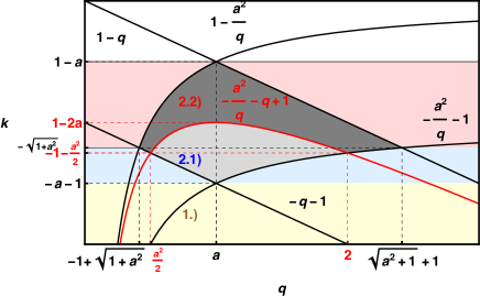
Figure 11: The condition (37) for the allowed region (light gray) bounded by $-1-q,1-q,1-a^{2}/q,-1-a^{2}/q$ and additionally to be larger than $1-a-a^{2}/q$ (gray). Depending on the maxima of the latter function (red) at $(a,1-2a)$ there are three cases, 1.2, 2.1,and 2.2.

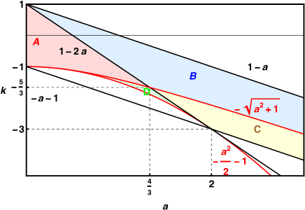
Figure 12: The condition (37) of figure 11 rearranged in $a-k$ plot yielding 4 different regions.

The allowed region is in a four-polygon and additionally above the curve $1-a^{2}/q-q$. Due to its maxima at $(a,1-2a)$ we have 3 cases:

• $1-2a<-1-a$ which means $a>2$ and we have

  $$-1-a<k<-\sqrt{1+a^{2}}:-1-k<q<-{a^{2}\over 1+k}$$

  $$-\sqrt{1+a^{2}}<k<1-a:{a^{2}\over 1-k}<q<1-k$$ (38)

• $-1-a<1-2a$ which means $\frac{4}{3}<a<2$ and

  $$-1-{a^{2}\over 2}<k<1-2a:$$

  $$\qquad\qquad-1-k<q<q_{2}\quad{\rm or}\quad q_{1}<q<-{a^{2}\over 1+k}$$

  $$1-2a<k<-\sqrt{1+a^{2}}:-1-k<q<-{a^{2}\over 1+k}$$

  $$-\sqrt{1+a^{2}}<k<1-a:{a^{2}\over 1-k}<q<1-k$$ (39)

• $-\sqrt{1+a^{2}}<1-2a<1-a$ which yields $0<a<\frac{4}{3}$ and

  $$-1-{a^{2}\over 2}<k<-\sqrt{1+a^{2}}:$$

  $$\qquad\qquad-1-k<q<q_{2}\quad{\rm or}\quad q_{1}<q<-{a^{2}\over 1+k}$$

  $$-\sqrt{1+a^{2}}<k<1-2a:$$

  $$\qquad\qquad{a^{2}\over 1-k}<q<q_{2}\quad{\rm or}\quad q_{1}<q<1-k$$

  $$-\sqrt{1+a^{2}}<k<1-a:{a^{2}\over 1-k}<q<1-k$$ (40)

with the two crossing points of the $1-q-a^{2}/q$ curve with the horizontal $k$-line

$$q_{1/2}={1-k\over 2}\pm\sqrt{{(1-k)^{2}\over 4}-a^{2}}.$$ (41)

Eq. (40) provides the integration limits for $q$ of

$$\Phi(q) ={s^{4}r_{s}^{2}\over\pi^{3}}\int\limits^{q}d\bar{q}{v_{\bar{q}}\over|\bar{q}|}\left(sv_{q}-v_{a^{2}\over q}\right)$$

$$={s^{4}r_{s}^{2}\over\pi^{3}}\left\{\begin{array}[]{cc}\ln q&{\rm contact}\cr\frac{\ln\left(\frac{q^{2}}{\kappa^{2}+q^{2}}\right)}{\kappa^{2}}+\frac{iF\left(i{\rm arsinh}\left(\frac{q}{\kappa}\right)|\frac{\kappa^{4}}{a^{4}}\right)}{a^{2}}&{\rm pot.}(\ref{pot})\end{array}\right..$$ (44)

witt the elliptic integral of first kind

$$F(a|m)=\int\limits_{0}^{a}{d\theta\over\sqrt{1-m\sin^{2}\theta}}.$$ (45)

Plotting the cases 1., 2.1, and 2.2. and regrouping with respect to $k$ one sees in figure 12 that 4 areas $A-D$ appear with 3 combinations of

$${\rm area}\,A,B:\, \Phi(1-k)-\Phi\left({a^{2}\over 1-k}\right)$$

$${\rm area}\,A,D:\, \Phi(q_{2})-\Phi(q_{1})$$

$${\rm area}\,C,D:\, \Phi\left({a^{2}\over-1-k}\right)-\Phi(-1-k)$$ (46)

Remembering that in order to include the $q<0$ part we have to add all expressions for $k\to-k$ which provides finally the cases (10).

Appendix B $q$-integration for $\sigma^{>}$

The occupation factors in (19) lead after $\delta$-integration for $p$ to the conditions

$$1-n_{p-q}: k<-1+{\Omega\over 2q}\quad{\rm or}\quad 1+{\Omega\over 2q}<k$$ (47)

$$n_{k+q}: k<-1-q\quad{\rm or}\quad 1-q<k$$

$$n_{p}: -1-q+{\Omega\over 2q}<k<1-q+{\omega\over 2q}<k$$

which together allows four possibilities for the range of $k$

$${\rm max}\!\left(\!-1\!+\!{\Omega\over 2q}\!-\!q\!\right)\!<\!k\!<\!{\rm min}\!\left(-\!1\!-\!q,\!1\!+\!{\Omega\over 2q}\!-\!q,-1\!+\!{\Omega\over 2q}\!\right)$$ (48)

$${\rm or}$$

$${\rm max}\!\left(\!-1\!+\!{\Omega\over 2q}\!-\!q,1\!+\!{\Omega\over 2q}\!\right)\!<\!k\!<\!{\rm min}\!\left(-\!1\!-\!q,\!1\!+\!{\Omega\over 2q}\!-\!q\!\right)$$

$${\rm or}$$

$${\rm max}\!\left(\!-1\!+\!{\Omega\over 2q}\!-\!q,1-q\!\right)\!<\!k\!<\!{\rm min}\!\left(\!-1\!+\!{\Omega\over 2q},1\!+\!{\Omega\over 2q}\!-\!q\!\right)$$ (49)

$${\rm or}$$

$${\rm max}\!\left(\!-1\!+\!{\Omega\over 2q}\!-\!q,1-q,1\!+\!{\Omega\over 2q},\!\right)\!<\!k\!<\!{\rm min}\!\left(\!1\!+\!{\Omega\over 2q}\!-\!q\!\right)$$

where the second and fourth line is not possible to complete due to the last expressions on left and right side $1\!+\!{\Omega\over 2q}\!<\!k\!<\!1\!+\!{\Omega\over 2q}\!-\!q$. The first line is only possible to complete for $\Omega<0$ since $-1\!+\!{\Omega\over 2q}\!-\!q\!<\!k\!<\!-\!1\!-\!q$ and the third line only for $\Omega>0$ due to $1\!-\!q\!<\!k\!<\!1\!+\!{\Omega\over 2q}\!-\!q\!$. Therefore we have two cases:

B.0.1 $\Omega=\omega-k^{2}<0$

Discussing first the case (48) and setting

$$a=\sqrt{-\Omega/2}$$ (50)

the area is plotted in figure 13.

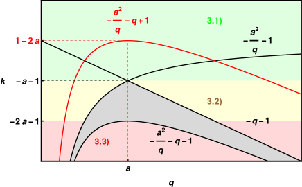
Figure 13: The condition (48) for the allowed region (light gray) bounded by $-1-q,-1-a^{2}/q,-1-a^{2}/q-q$ and additionally to be smaller than $1-q-a^{2}/q$ (red line). Depending on the maxima of the latter function (red) at $(a,1-2a)$ there are three cases (3.1)-(3.3).

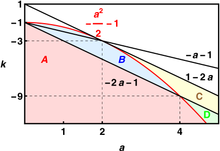
Figure 14: The condition (48) of figure 13 rearranged in $a-k$ plot yielding 4 different regions.

The allowed region is additionally below the curve $-1-a^{2}/q-q$. Due to its maxima at $(a,1-2a)$ we have 3 cases:

• $1-2a<-1-a$ which means $a>2$ and we have

  $$-\infty<k<-1-2a:$$

  $$\qquad-{a^{2}\over 1+k}<q<q_{4}\quad{\rm or}\quad q_{3}<q<-1-k$$

  $$-1\!-\!2a<k<-1\!-\!a:-{a^{2}\over 1\!+\!k}<q<-1\!-\!k$$ (51)

• $-1-2a<-1-a$ and $-1-a^{2}/2>-1-2a$ which means $2<a<4$ and

  $$-\infty<k<-1-2a:$$

  $$\qquad-{a^{2}\over 1+k}<q<q_{4}\quad{\rm or}\quad q_{3}<q<-1-k$$

  $$-1-2a<k<-1-{a^{2}\over 2}:-{a^{2}\over 1+k}<q<-1-k$$

  $$-1-{a^{2}\over 2}<k<1-2a:q_{2}<q<q_{1}$$ (52)

• $-1-{a^{2}\over 2}<-1-2a$ which yields $4<a$ and

  $$-1-{a^{2}\over 2}<k<-1-2a:$$

  $$\qquad q_{2}<q<q_{4}\quad{\rm or}\quad q_{3}<q<q_{1}$$

  $$-1-2a<k<1-2a:q_{2}<q<q_{1}$$

  $$-\infty<k<-1-{a^{2}\over 2}:$$

  $$\qquad-{a^{2}\over 1-k}<q<q_{4}\quad{\rm or}\quad q_{3}<q<-1-k$$ (53)

with the two crossing points of the $\pm 1-q-a^{2}/q$ curves with the horizontal $k$-line of (41)

$$q_{3/4}={-1-k\over 2}\pm\sqrt{{(1+k)^{2}\over 4}-a^{2}}.$$ (54)

In figure 14 we plot these ranges and obtain 4 areas $A-D$ with 3 combinations of

$${\rm area}\,A,B:\, \Phi(-1-k)-\Phi\left({a^{2}\over-1-k}\right)$$

$${\rm area}\,A,D:\, \Phi(q_{4})-\Phi(q_{3})$$

$${\rm area}\,C,D:\, \Phi\left(q_{1}\right)-\Phi(q_{2})$$ (55)

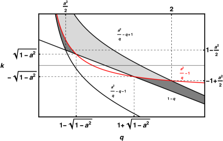
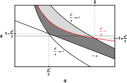
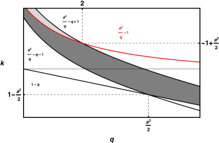
Figure 15: The condition (49) for the allowed region (light gray) bounded by $-1-q,-1-a^{2}/q,-1-a^{2}/q-q$ and additionally to be smaller than $a^{2}/q-1$ (gray). Depending on the latter function (red) there are three cases 4.1)-4.3) from top to bottom.

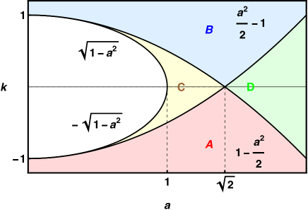
Figure 16: The condition (48) of figure 15 rearranged in $a-k$ plot yielding 4 different regions.

Again we have to add all expressions for $k\to-k$ to get finally the cases (20)

B.0.2 $\Omega=\omega-k^{2}>0$

The condition (49) and setting $a=\sqrt{\Omega/2}$ can be seen in figure 15. The allowed region is additionally below the curve $-1-a^{2}/q-q$ and we have 3 cases:
4.1) ${a^{2}\over 2}<1-\sqrt{1-a^{2}}<1+\sqrt{1-a^{2}}<2$ which means $a<1$ and we have

$$-\infty<k<-1+{a^{2}\over 2}:1-k<q<q_{7}$$

$$-1\!+\!{a^{2}\over 2}<k<-\sqrt{1-a^{2}}:1\!-\!k<q<{a^{2}\over 1\!+\!k}$$

$$\sqrt{1-a^{2}}<k<1\!-\!{a^{2}\over 2}:1\!-\!k<q<{a^{2}\over 1\!+\!k}$$

$$1\!-\!{a^{2}\over 2}<k<\infty:q_{8}<q<{a^{2}\over 1\!+\!k}$$ (56)

4.2) $1-a^{2}/2>-1+a^{2}/2>-\sqrt{1-a^{2}}$ which means $1<a<\sqrt{2}$ and

$$-\infty<k<-1+{a^{2}\over 2}:1-k<q<q_{7}$$

$$-1\!+\!{a^{2}\over 2}<k<1\!-\!{a^{2}\over 2}:1\!-\!k<q<{a^{2}\over 1\!+\!k}$$

$$1\!-\!{a^{2}\over 2}<k<\infty:q_{8}<q<{a^{2}\over 1\!+\!k}$$ (57)

4.3) $1-a^{2}/2<-1+a^{2}/2$ which means $\sqrt{2}<a$ and

$$-\infty<k<1-{a^{2}\over 2}:1-k<q<q_{7}$$

$$1\!-\!{a^{2}\over 2}<k<-1\!+\!{a^{2}\over 2}:q_{8}<k<q<q_{7}$$

$$-1\!+\!{a^{2}\over 2}<k<\infty:q_{8}<q<{a^{2}\over 1\!+\!k}$$ (58)

with the two crossing points of the $\pm 1-q+a^{2}/q$ curve with horizontal line

$$q_{7/8}={\pm 1-k\over 2}+\sqrt{{(1\mp k)^{2}\over 4}+a^{2}}.$$ (59)

In figure 16 we plot these ranges and obtain 4 areas $A-D$ with the combinations

$${\rm area}\,A\,: \Phi\left(q_{7}\right)-\Phi(1-k)$$

$${\rm area}\,B\,: \Phi\left({a^{2}\over 1+k}\right)-\Phi(q_{8})$$

$${\rm area}\,C\,: \Phi\left({a^{2}\over 1+k}\right)-\Phi(1-k)$$

$${\rm area}\,D\,: \Phi\left(q_{7}\right)-\Phi(q_{8}).$$ (60)

Again we have to add all expressions for $k\to-k$ to get the cases (22).

Appendix C Real part of selfenergy

We calculate the Hilbert transform (1) by interchanging integration orders

$$\sigma(q,\omega) = \int\limits_{-\infty}^{\infty}{d\bar{\omega}\over 2\pi}{\sigma^{<}(q,\bar{\omega})\over\omega-\bar{\omega}}$$ (61)

$$= \int\limits_{0}^{\infty}{dx\over 2\pi}{\sigma^{<}(q,x)\over{\cal O}+x}+\int\limits_{-\infty}^{\infty}{dx\over 2\pi}{\sigma^{>}(q,x)\over{\cal O}-x}$$

$$= {s^{4}r_{s}^{2}\over 2\pi^{4}}\int\limits_{u}^{o}{dq}{v_{q}\over q}\int\limits_{x_{u}}^{x_{o}}{dx\over{\cal O}+x}\left(sv_{q}-v_{x\over q}\right)$$

where the integration limit of $q$ according to (10) are interchanged with $a^{2}=x=(k^{2}-\omega)/2$ integration leading to the limits summarized in table 1. We have abbreviated

$${\cal O}=(\omega-k^{2})/2\gtrless 0$$ (62)

and used a transformation of $x\to-x$ in the part for $\sigma^{>}$.

As example, the case

$$0<k<1 \Phi(1-k)-\Phi\left({a^{2}\over 1-k}\right)\,{\rm for}\, 0\!<\!a^{2}\!<\!(1\!-\!k)^{2}$$ (63)

leads to

$$\int\limits_{0}^{(1-k)^{2}}{dx\over{\cal O}+x}\int\limits_{x\over 1-k}^{1-k}{dq\over q}v_{q}(sv_{q}-v_{x\over q})$$

$$=\int\limits_{0}^{1-k}{dq\over q}v_{q}\int\limits_{0}^{(1-k)q}{dx\over{\cal O}+x}(sv_{q}-v_{x\over q})$$ (64)

as represented in first line of table 1. Working out all cases of (10) is tedious but straight by just painting all the corresponding curves. Summing up the contributions according to the range of $k$ we obtain (28) which shows that the ranges $1<k<3$ and $k>3$ are identically as it should since we have only $k=1(k_{f})$ as exceptional point.

Table 1: Integration limits of 61 where we use the abbreviations $[ij]=-q^{2}+ikq+jq$ and $(ij)=ikq+jq$.

$\sigma^{<}$	$u$	$o$	$x_{u}$	$x_{o}$
$0<k<1$
	$0$	$1-k$	$0$	$(-+)$
	$1-k$	$0$	$0$	$[-+]$
	$0$	$1+k$	$0$	$(++)$
	$1+k$	$0$	$0$	$[++]$
$1<k<3$
	$2$	$k+1$	$(+-)$	$k^{2}-1$
	$k-1$	$2$	$[++]$	$(++)$
	$k-1$	$k+1$	$k^{2}-1$	$(++)$
$3<k$
	$k-1$	$k+1$	$(--)$	$(+-)$

$\sigma^{>}$	$u$	$o$	$x_{u}$	$x_{o}$
$0<k<1$
	$1+k$	$2$	$[--]$	$(--)$
	$1-k$	$1+k$	$(+-)$	$(--)$
	$2$	$\infty$	$[--]$	$[++]$
	$2$	$\infty$	$[-+]$	$[+-]$
$1<k<3$
	$0$	$2$	$0$	$(--)$
	$1+k$	$2$	$[-+]$	$0$
	$0$	$k+1$	$[--]$	$0$
	$k+1$	$\infty$	$[--]$	$[++]$
	$k+1$	$\infty$	$[+-]$	$[-+]$
	$0$	$k-1$	$[+-]$	$(+-)$
$3<k$
	$0$	$2$	$0$	$(--)$
	$1+k$	$2$	$[-+]$	$0$
	$0$	$k+1$	$[--]$	$0$
	$k+1$	$\infty$	$[--]$	$[++]$
	$k+1$	$\infty$	$[+-]$	$[-+]$
	$0$	$k-1$	$[+-]$	$0$
	$0$	$2$	$0$	$(+-)$
	$2$	$k-1$	$2(k-1)$	$[++]$

References

(1)
R. Saito, G. Dresselhaus, and M. S. Dresselhaus, Physical Properties of
Carbon Nanotubes (Imperial College Press, London, 1998).
(2)
M. Bockrath et al., Nature 397, 598 (1999).
(3)
H. Ishii et al., Nature 426, 540 (2003).
(4)
M. Shiraishi and M. Ata, Sol. State Commun. 127, 215 (2003).
(5)
F. P. Milliken, C. P. Umbach, and R. A. Webb, Sol. State Commun. 97, 309 (1996).
(6)
S. S. Mandal and J. K. Jain, Sol. State Commun. 118, 503 (2001).
(7)
A. M. Chang, Rev. Mod. Phys. 75, 1449 (2003).
(8)
J. Schäfer et al., Phys. Rev. Lett. 101, 236802
(2008).
(9)
Y. Huang et al., Science 294, 1313 (2001).
(10)
H. Monien, M. Linn, and N. Elstner, Phys. Rev. A 58, R3395
(1998).
(11)
A. Recati, P. O. Fedichev, W. Zwerger, and P. Zoller, J. Opt. B: Quantum
Semiclass. Opt. 5, S55 (2003).
(12)
H. Moritz et al., Phys. Rev. Lett. 94, 210401 (2005).
(13)
A. Nitzan and M. A. Ratner, Science 300, 1384 (2003).
(14)
T. Schätz, U. Schramm, and D. Habs, Nature 412, 717 (2001).
(15)
U. Schramm, T. Schätz, M. Bussmann, and D. Habs, Plasma Phys. Control
Fusion 44, B375 (2002).
(16)
J. M. Luttinger, J. Math. Phys. 4, 1154 (1963).
(17)
A. Luther and I. Peschel, Phys. Rev. B 9, 2911 (1974).
(18)
U. Eckern and P. Schwab, phys. stat. sol. (b) 244, 2343 (2007).
(19)
I. E. Dzyaloshinskii and A. I. Larkin, Sov. Phys. JETP 38, 202 (1974).
(20)
L. Rammelmüller, W. J. Porter, J. Braun, and J. E. Drut, Phys. Rev. A 96, 033635 (2017).
(21)
J.-F. Pan, J.-J. Luo, and X.-W. Guan, Communications in Theoretical Physics
74, 125802 (2022).
(22)
F. H. L. Eßler et al., The One-dimensional Hubbard Model
(Cambridge University Press, Cambridge, 2010).
(23)
X.-W. Guan, M. T. Batchelor, and C. Lee, Rev. Mod. Phys. 85, 1633
(2013).
(24)
A. Luther, Phys. Rev. B 15, 403 (1977).
(25)
J. Sólyom, Adv. Phys. 28, 209 (1979).
(26)
D. B. Gutman, Y. Gefen, and A. D. Mirlin, Phys. Rev. B 81, 085436
(2010).
(27)
F. D. M. Haldane, Phys. Rev. Lett. 47, 1840 (1981).
(28)
V. J. Emery, in Highly Conducting One-Dimensional Solids, edited by J.
Devreese and et al. (Plenum Press, New York, 1979), p. 247.
(29)
A. Girdhar et al., Phys. Rev. B 105, 115140 (2022).
(30)
R. M. Lee and N. D. Drummond, Phys. Rev. B 83, 245114 (2011).
(31)
P. F. Loos and M. W. Gill, WIREs Comput. Mol. Sci. 6, 410 (2016).
(32)
P.-F. Loos, The Journal of Chemical Physics 138, 064108 (2013).
(33)
K. Morawetz, V. Ashokan, R. Bala, and K. N. Pathak, Phys. Rev. B 97,
155147 (2018).
(34)
S. Giorgini, L. P. Pitaevskii, and S. Stringari, Rev. Mod. Phys. 80,
1215 (2008).
(35)
K. Morawetz, Eur. Phys. J. B 96, 95 (2023).
(36)
G. Schliecker, K. D. Schotte, B. Horvatic, and V. Zlatic, Journal of Physics:
Condensed Matter 7, 7969 (1995).
(37)
J. Voit, Rep. Prog. Phys. 57, 977 (1994).
(38)
T. Giamarchi, Chem. Rev. 104, 5037 (2004).
(39)
G. F. Giuliani and G. Vignale, Quantum theory of electron liquid
(Cambridge University Press, Cambridge, 2008).
(40)
K. Morawetz, Interacting systems far from equilibrium - quantum kinetic
theory (Oxford University Press, Oxford, 2017).
(41)
A. Theumann, J. Math. Phys. 8, 2460 (1967).
(42)
V. Garg, R. K. Moudgil, K. Kumar, and P. K. Ahluwalia, Phys. Rev. B 78,
045406 (2008).
(43)
P. Schlottmann, Phys. Rev. B 16, 2055 (1977).
(44)
K. Yokoyama, Journal of the Physical Society of Japan 70, 2825 (2001).
(45)
O. Gamayun, A. G. Pronko, and M. B. Zvonarev, Nuclear Physics B 892, 83
(2015).
(46)
S. Liang, D. Zhang, and W. Chen, J. Phys. Condens. Matter 31, 185601
(2019).
(47)
V. Ashokan, R. Bala, K. Morawetz, and K. N. Pathak, Phys. Rev. B 101,
075130 (2020).
(48)
J. Voit, Phys. Rev. B 47, 6740 (1983).
(49)
F. H. L. Essler, Phys. Rev. B 81, 205120 (2010).
(50)
J. Voit, Phys. Rev. B 47, 6740 (1993).
(51)
V. Meden and K. Schönhammer, Phys. Rev. B 46, 15753 (1992).
(52)
J. Voit, Journal of Physics: Condensed Matter 5, 8305 (1993).
(53)
H. Tajima, S. Tsutsui, and T. M. Doi, Phys. Rev. Res. 2, 033441 (2020).