Stellar Populations in STARFORGE: The Origin and Evolution of Star Clusters and Associations

Abstract

Most stars form in highly clustered environments within molecular clouds, but eventually disperse into the distributed stellar field population. Exactly how the stellar distribution evolves from the embedded stage into gas-free associations and (bound) clusters is poorly understood. We investigate the long-term evolution of stars formed in the STARFORGE simulation suite – a set of radiation-magnetohydrodynamic simulations of star-forming turbulent clouds that include all key stellar feedback processes inherent to star formation. We use Nbody6++GPU to follow the evolution of the young stellar systems after gas removal. We use HDBSCAN to define stellar groups and analyze the stellar kinematics to identify the true bound star clusters. The conditions modeled by the simulations, i.e., global cloud surface densities below 0.15 g cm^-2 , star formation efficiencies below 15%, and gas expulsion timescales shorter than a free fall time, primarily produce expanding stellar associations and small clusters. The largest star clusters, which have $\sim$1000 bound members, form in the densest and lowest velocity dispersion clouds, representing $\sim$32 and 39% of the stars in the simulations, respectively. The cloud’s early dynamical state plays a significant role in setting the classical star formation efficiency versus bound fraction relation. All stellar groups follow a narrow mass-velocity dispersion power law relation at 10 Myr with a power law index of 0.21. This correlation result in a distinct mass-size relationship for bound clusters. We also provide valuable constraints on the gas dispersal timescale during the star formation process and analyze the implications for the formation of bound systems.

1 Introduction

Star formation is the result of the complex interplay between physical processes over a wide range of spatial scales within giant molecular clouds (GMCs) undergoing gravitational collapse. One key ingredient in this process is turbulence, which is characterized by large-scale random motions that cascade down to smaller scales (e.g., Girichidis et al., 2020). As cloud collapse proceeds, turbulent motions seed hierarchical fragmentation, leading to stellar groups of thousands rather than a small number of isolated stars (Pokhrel et al., 2018). Depending on the parent cloud properties, the star-formation process produces stellar distributions spanning a broad range of sizes and scales, from massive bound clusters and unbound associations down to multiple and single-star systems (Krause et al., 2020; Pokhrel et al., 2020).

As star formation models have become more realistic and kinematic observations have become more detailed, there is increasing evidence that a significant fraction of stars do not form in bound configurations (Ward et al., 2020; Wright et al., 2022), which we henceforth refer to as clusters (Krumholz et al., 2019; Chevance et al., 2022). While most stars in the galaxy may have formed in groups of dozens to thousands of stars (Lada & Lada, 2003), the vast majority are currently not in clusters but rather compose the distributed Milky Way field population. The statistical absence of relatively old, gas-free star clusters compared to the abundance of embedded star clusters suggests that most stellar groups dissolve when natal gas from their host cloud is dispersed due to stellar feedback (Krumholz et al., 2019; Krause et al., 2020). However, observationally determining whether a given group of young stars is truly bound has historically been challenging given the difficulty of obtaining detailed kinematic information (Gieles & Portegies Zwart, 2011).

Early models of stellar systems using smooth spherical stellar distributions, show that two key factors inhibit the formation of a bound cluster: low star formation efficiency (SFE), whereby most of the binding potential is lost with the ejected gas, and rapid gas dispersal, whereby stars do not have time to adapt their orbits to the new potential (Tutukov, 1978; Hills, 1980; Adams, 2000; Baumgardt & Kroupa, 2007; Proszkow & Adams, 2009; Pfalzner & Kaczmarek, 2013; Smith et al., 2013a). Subsequent studies have demonstrated that the introduction of stellar substructure, motivated by the evidence of filamentary structure in star-forming regions, produces large variations in the dynamical state of the stars, as the groups transition from substructured to spherical configurations through dynamical interactions. Such relaxation produces sub-virial and super-virial dynamical states that may help or hinder a star cluster’s ability to retain members (Goodwin, 2009; Lee & Goodwin, 2016; Farias et al., 2018; Li et al., 2019).

Furthermore, the structure and dynamics of how the gas interacts with the stars is such a complex process that most prior theoretical work adopts a simplified and somewhat arbitrary description for the parent gas cloud or neglects key sources of stellar feedback, such as radiation pressure, photoionization, and stellar winds; that affects its dynamics and the subsequent gas dispersal (e.g Pelupessy & Portegies Zwart 2012; Sills et al. 2018; Farias et al. 2018, also see review by Krause et al. 2020 ). Consequently, the interplay between these different stellar feedback processes and the substructures formed by the stars and gas play a crucial role in setting the stability of young stellar systems and determining whether a star cluster or association forms.

The recently developed STAR FORmation in Gaseous Environments (STARFORGE) framework (Grudić et al., 2021a, hereafter Paper I) has made significant progress in modeling the evolution of star-forming clouds, including all relevant forms of stellar feedback. Additionally, since STARFORGE is capable of forming individual stars down to $M_{\star}\sim 0.1~{}M_{\rm odot}$ it is able to follow stellar dynamics and the resulting stellar distribution until the natal gas is dispersed (Guszejnov et al., 2021; Grudić et al., 2022, hereafter Paper II and Paper III , respectively). In the following paper series, the STARFORGE group modeled molecular clouds with a range of initial conditions and studied the role of feedback on the origin of stellar clustering (Guszejnov et al., 2022a, hereafter Paper IV), the stellar IMF (Guszejnov et al., 2022b, hereafter Paper V), and the evolution of stellar multiplicity (Guszejnov et al., 2023, hereafter Paper VI). The models explored the impact of variations in the dynamical equilibrium of the cloud, magnetic field strength, interstellar radiation field, metallicity, gas density and cloud mass. Altogether the simulated clouds produce a significant range of stellar distributions, where most appear to be unbound at the end of the calculation (; ). In particular Paper IV used the clustering algorithm DBSCAN to identify stellar groups and follow their dynamical evolution. They found that smaller groups frequently merge to form larger complexes, which later fragment and expand during the post-collapse phase where most of gas is dispersed by stellar feedback. However, the subsequent evolution and final state of the stellar groups was not modeled.

In this work, we examine the long-term evolution of the stellar distributions from the STARFORGE simulations (i.e., once the remaining cloud gas is dispersed) to characterize their properties and linking these, when possible, to their parent clouds. We follow the terminology convention that a star cluster is a group of stars that are gravitationally bound, while a stellar association is a group of stars that are not bound but are identified as a single system (e.g., using a clustering algorithm, see below, Krumholz et al., 2019). We reserve group as a general term, which encompasses both clusters and associations.

In § 2 we describe the numerical codes used in this work and summarize our methods. We present our analysis and results in § 3, followed by discussion in § 4, and conclusions in § 5.

2 Methods

2.1 STARFORGE

In this paper, we follow the evolution of the stellar complexes formed in the STARFORGE simulations (; ). STARFORGE is a numerical framework developed to model the formation of stars from their parent Giant Molecular Clouds (GMCs), including the most complete set of physical processes to date over a wide dynamical range (Paper I). These physical processes include all key sources of stellar feedback such as protostellar outflows, stellar winds, radiation pressure, photoionization and supernovae.

The simulations are run with the GIZMO code and adopt the Lagrangian meshless finite-mass (MFM) method for magneto-hydrodynamics (MHD) under the ideal MHD approximation (Hopkins, 2015, 2016). Self-gravity is modeled using an improved version of the Barnes & Hut tree algorithm (Springel, 2005). The sink particle orbital integration uses an order four Hermite integrator, allowing the correct integration of binaries and higher order multiples. Accreting sink particles have a fixed radius of 18 AU. This radius is also used as a softening length for close encounters. As sink particles (protostars) form, they follow the protostellar evolution model from Offner et al. (2009). Cooling and heating are treated utilizing the thermo-chemistry module from Hopkins et al. (2023), which includes metallicity-dependent cooling and heating from $T=2.7-10^{10}$ K, recombination, thermal bremsstrahlung, metal lines, molecular lines, fine structure and dust collisional processes (see references in Hopkins et al., 2023, for details). Radiative processes are also included, accounting for photon transport, absorption and emission in 5 bins covering the electromagnetic spectrum. Sources of radiation include stars (including both the accretion and internal stellar luminosities), thermal dust emission, and gas continuum and line processes modeled by the cooling treatment. Other important forms of stellar feedback implemented in STARFORGE are stellar winds from massive stars, following the prescription described in Paper I, and protostellar jets, which are implemented by ejecting a fraction of the accreted material along the rotational axis of the protostar (Cunningham et al., 2011). In addition, stars more massive than 8 $M_{\sun}$ will undergo a supernova explosion at the end of their lifetime (at least 3 Myr), which is implemented as an isotropic ejection of all mass with a total energy of $E_{\rm SN}=10^{51}$ erg.

2.1.1 STARFORGE simulations as initial conditions

We post-process a selected set of simulations where the fiducial set of initial conditions is presented in Paper III, and simulations with variations on the fiducial parameters are presented in Paper V. The simulations begin with a uniform sphere of gas of mass $M_{0}=20,000\,M_{\sun}$, radii of $R_{\rm cloud}=3-30$ pc and $T=10$ K; the cloud is surrounded by warm ($T=10^{4}$ K), diffuse gas that is 1000 times less dense so that the cloud is initially in thermal pressure equilibrium with the ambient medium. The cloud turbulence is initialized with a Gaussian random velocity field with a power spectrum $E_{k}\propto k^{-2}$ scaled to match the turbulent virial parameter ($\alpha_{\rm turb}$), which represents the relative importance of the cloud’s kinetic energy to gravity, defined as (Bertoldi & McKee, 1992):

$$\alpha_{\rm turb} = \frac{5||\mathbf{v}_{\rm turb}||^{2}R_{\rm cloud}}{3GM_{0}},$$ (1)

where $\mathbf{v}_{\rm turb}$ and $R_{\rm cloud}$ are the turbulent velocity field and cloud radius, respectively. As a fiducial value, Paper III set $\alpha_{\rm turb}=2$, which is characteristic of GMCs in the Milky Way (see Larson, 1981; Chevance et al., 2022).

In these models, the importance of the magnetic field relative to the gravitational energy is parameterized by $\mu$ as:

$$\mu = c_{1}\sqrt{\frac{-E_{\rm grav}}{E_{\rm mag}}},$$ (2)

where $E_{\rm grav}$ and $E_{\rm mag}$ are the gravitational and magnetic energy, respectively, and $c_{1}\approx 0,42$ normalization constant such that $\mu=1$ represents a critically stable homogeneous sphere in a uniform magnetic field (Mouschovias et al., 1976). The fiducial simulation value is $\mu=4.2$ i.e. $E_{\rm mag}=0.1E_{\rm grav}$. The simulations include an external heating source representing the interstellar radiation field (ISRF), using the default assumption of solar neighbourhood conditions (Draine, 2010). Dust abundances in the clouds assume solar metallicity with a dust-to-gas ratio of 0.01.

Table 1 summarizes the STARFORGE simulations used in this work. The fiducial model represents the standard set of parameters used in Paper III and Paper V, i.e., a $M_{0}=20,000\,M_{\sun}$ turbulent molecular cloud that is marginally bound ($\alpha_{\rm turb}=2$) with size $R_{\rm cloud}=10$ pc and $\mu=4.2$ with local (solar neighborhood) ISRF conditions and solar metallicity. We also investigate ten variations of the standard model: low and high turbulent velocity field runs alpha1 ($\alpha_{\rm turb}=1$) and alpha4 ($\alpha_{\rm turb}=4$), respectively; two cases with 10 (Bx10) and 100 (Bx100) times stronger magnetic fields and two models with ten times higher and lower densities, i.e., clouds with $R_{\rm cloud}=3$ pc (R3) and $R_{\rm cloud}=30$ pc (R30); ISRF increased by a factor 10 (ISRFx10) and 100 (ISRFx100); and two models with gas metallicity decreased by a factor ten (Z01) and hundred (Z001) relative to the fiducial solar value.

The global evolution follows the cloud collapse; most stars in the simulation form at about two initial freefall times. The clouds have an average star formation efficiency (SFE) on the order of $\sim 10\%$. Radiative and wind feedback from the newly formed massive stars start to disperse the cloud and reduce star formation around 2 freefall times. Given their high numerical cost, the simulations are chosen to end after the first supernova goes off. At this point star formation has mostly ceased and most of the gas was already dispersed from the region. Our calculations pick up where the STARFORGE simulations end ($t_{\rm init}$, see Table 1), and we continue to follow the evolution of the formed stellar groups using the direct $N$-body code Nbody6++GPU (Aarseth, 2003; Wang et al., 2015) without the gas particles. We evolve these stellar distributions for 200 Myr at which point the stellar groups can be clearly classified as either clusters or associations.

		Cloud initial conditions					Properties at $t_{\rm init}$
Model	# of runs	$M_{0}$	$R_{\rm cloud}$	$\alpha_{\rm turb}$	$\mu$		$t_{\rm init}$	SFE	LSF	$N_{*}$	$t_{\rm exp}$
		[$M_{\sun}$]	[pc]				[Myr]				[Myr]
fiducial	3	$2\times 10^{4}$	10	2	4.2		$10.1\pm 0.9$	$0.080\pm 0.003$	$0.97\pm 0.04$	$2034\pm 131$	$5.0\pm 0.9$
alpha1	1	$2\times 10^{4}$	10	1	4.2		9.0	0.11	0.99	2464	$5.0$
alpha4	1	$2\times 10^{4}$	10	4	4.2		17.1	0.039	0.98	1220	$7.9$
R3	1	$2\times 10^{4}$	3	2	5.2		3.1	0.19	0.93	4450	$1.0$
R30	1	$2\times 10^{4}$	30	2	4.2		51.6	0.0099	0.99	358	$30$
Bx10	1	$2\times 10^{4}$	10	2	1.3		12.3	0.078	0.91	2246	$7.1$
Bx100	1	$2\times 10^{4}$	10	2	0.42		18.2	0.056	0.92	2415	$7.2$
ISRFx10	1	$2\times 10^{4}$	10	2	4.2		11.2	0.092	0.99	1835	$6.0$
ISRFx100	1	$2\times 10^{4}$	10	2	4.2		9.7	0.11	0.95	2116	$4.5$
Z01	1	$2\times 10^{4}$	10	2	4.2		10.9	0.045	0.15	1006	$5.5$
Z001	1	$2\times 10^{4}$	10	2	4.2		14.8	0.022	0.76	411	$6.0$

Table 1: STARFORGE simulation parameters for the different cloud models, which we label as shown in column 1. Second column shows the number of STARFORGE  simulations available for the set, including different initial turbulent seeds. Third to sixth columns show the parent cloud initial parameters, i.e. total mass ($M_{0}$), initial radii ($R_{\rm cloud}$), turbulent virial parameter ($\alpha_{\rm turb}$) and magnetic field strength parameter ($\mu$), respectively. Seventh column shows the end time of the STARFORGE simulations and the beginning of the $N$-body modeling, $t_{\rm init}$. The next three columns display the cloud properties at $t_{\rm init}$, i.e., global star formation efficiency (SFE) in column eight, stellar mass fraction within the half mass radius of the stars (referred as the local stellar fraction, LSF) in column nine, and the total number of stars at $t_{\rm init}$, $N_{*}$, in the tenth column. Last column shows the time in the STARFORGE run where the collapse phase of the cloud ends and expansion begins, $t_{\rm exp}$. Values for the fiducial model are averages over the three available simulations in the set.

2.2 Nbody6++GPU

2.2.1 Numerical Methods

Nbody6++GPU directly integrates the orbits of stars using a fourth-order Hermite integrator with a hierarchical block time-step method to increase performance. The block time-step method works by taking the time-step of individual stars from pre-defined time-step levels ($l$) with $\Delta t_{l}=\Delta t_{1}/2^{l-1}$ based on how quickly the orbits change. The calculation cost is reduced by using the Ahmad & Cohen (1973) neighbour scheme, which requires gathering a list of neighbours for each particle. Force updates for neighbours are calculated using smaller timesteps (referred to as irregular timesteps), and for all other stars, forces are updated on a larger timestep (referred to as regular timesteps).

Accurate integration of hard binary orbits and close encounters requires much shorter timesteps than those appropriate for the rest of the system and therefore necessitates special treatment. In contrast to the gravitational softening length adopted in STARFORGE, but commonly adopted by most direct N-Body integrators, Nbody6++GPU makes use of the Kustaanheimo & Stiefel (1965) algorithm (referred to as KS regularization). In this scheme a 3-dimensional space describing an isolated binary orbit is mapped onto a redundant 4-dimensional space on which the equations of motion are regular at collision, i.e. when the distance between the binary components reduce to zero. The implementation of KS regularizations in Nbody6++GPU uses generalizations of this method for perturbed binaries and higher order hierarchical multiples (chain regularizations, see Aarseth, 2003, and references therein). In addition, the code version we use here employs the GPU parallelization implemented by Wang et al. (2015).

2.2.2 $N$-body initial conditions and models

Our procedure following the evolution of the stellar systems begins with the last STARFORGE simulation snapshot, at which point stellar feedback has ejected most of the natal cloud gas. Table 1 records the time that corresponds to this last snapshot ($t_{\rm init}$). We feed the simulated stellar distributions in the final snapshots into the $N$-body solver after some additional corrections to account for the different methods and scopes of the two numerical codes, as discussed next.

The first challenge is the different treatment of close orbits in both codes. While Nbody6++GPU does not use any approximation for close encounters and binary orbits, STARFORGE uses a softening length that weakens the gravitational potential at close distances, such that the properties of close binaries found in the STARFORGE simulations will deform when placed in a regime with no approximations. Therefore we made corrections to the binary orbits before introducing them in the $N$-body simulations, as we describe in detail below.

A second complication is that some residual cloud gas remains in the vicinity of the stars we aim to model. While we restart from snapshots where the gas is mostly dispersed, the gravitational potential contributed by this gas could still influence the large-scale evolution of the modeled regions.

In the following sections, we explain how we address these complications during the initialization of Nbody6++GPU. To summarize our procedure, for each of the STARFORGE models under analysis, we follow two sets of simulations modeling distinct scenarios. In both cases, we input the corresponding binary-corrected stellar distribution into Nbody6++GPU and simulate the evolution for 200 Myr. In the simulation sets we refer to as NoExtPot we evolve the stars after gas expulsion, assuming complete gas clearance from the cluster, i.e. the stars evolve in isolation. In the second simulation set, which we refer to as ExtPot, we evolve the stars with a gas component remaining within the cluster, which we represent analytically.

2.2.3 Binary treatment

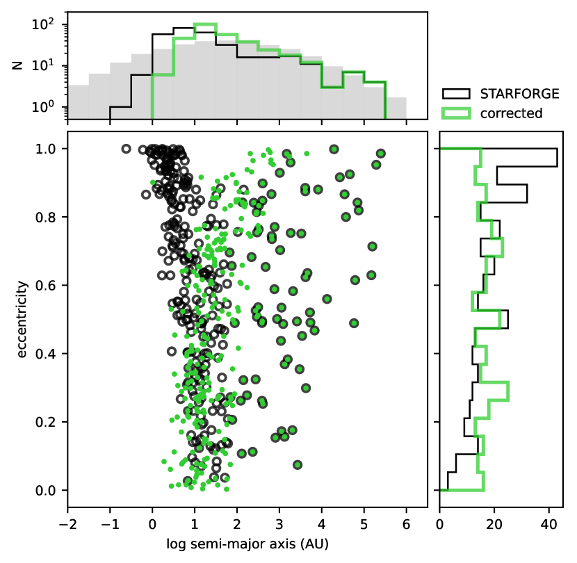
Figure 1: Semi-major axis versus eccentricity for binaries in the STARFORGE  simulations for the fiducial set at $t_{\rm init}=9.1$ Myr (black) and after correcting their orbits (green). Under-resolved binary orbits produce highly eccentric orbits given their low orbital velocities, which is caused by using their velocity orbits under a softening length approximation. We correct the orbit of any binary with current separation below 60 $\rm AU$. The gray shaded area in the top panel shows the expected semi-major axis distribution for solar-type stars from Raghavan et al. (2010).

Binary and multiple systems are a natural outcome of the star formation process (Offner et al., 2022). About half of the stars formed in the STARFORGE calculations are members of multiple systems, with overall statistics that are in reasonable agreement with the observed multiplicity and companion star fractions when the periastron is larger than the softening radius (Paper VI). From a numerical standpoint, the dynamics of binary stars are challenging to integrate given their large range of timescales, where the shortest periods are on the order of days versus the typical dynamical timescale of a star-forming cloud, which is on the order of millions of years. Nbody6++GPU solves this problem by using KS regularization routines, however such routines are less advantageous in tightly-coupled, multi-physics setups, which have additional overheads and lack a clear separation of timescales between binary and gas evolution. The STARFORGE calculations are limited by mass resolution, and equivalently by a minimum scale length, under which any physical process will be under-resolved, including binary orbits. STARFORGE adopts a more practical approach, which uses a conveniently chosen softening length, to avoid integrating highly expensive orbits on a regime that is already under-resolved.

The STARFORGE standard mass resolution used in all models studied here is $10^{-3}M_{\sun}$. Paper I showed that the smallest Jeans resolved spatial resolution is of order $\sim 20\,\rm AU$, which is adopted as the softening length. Therefore, any binary with pericenter close to $20\,\rm AU$ is under-resolved, and we must correct the orbit velocities before evolving these binaries with the $N$-body solver. We apply the correction to all binaries below a force deviation tolerance of 10%, i.e., any pair with current separation below 60 $\rm AU$.

Affected binaries have orbital velocities that are too slow, given the weakened gravitational potential used in the hydrodynamical solver. Consequently, to a dedicated $N$-body solver, they will appear to have artificially eccentric orbits, and therefore artificially small semimajor axes.

We assume that all gravitationally bound stellar pairs produced in the STARFORGE  calculations are true binaries, and we correct their orbits by the following procedure:

1. We assign a new eccentricity ($e$), drawn from a uniform distribution.

2. We retain their current separation but adopt it as the peri-apsis. In this way we avoid possible artificial collisions due to highly eccentric orbits.

3. Using the current eccentricity and peri-apsis, we derive the new semi-major axis ($a$, which is greater than the original), and obtain the magnitude of the velocity at the peri-apsis position.

4. We find the velocity vector direction by conserving the original orbital plane. We obtain the original angular momentum vector, and the new relative velocities are assigned such that the direction of the angular momentum vector and the center of mass of the binary are the same as the original.

Figure 1 shows an example distribution of binaries, where after correcting the binary orbits, the semi-major axes increase and eccentricities transform from a skewed distribution peaked at $e=1$ into a uniform one.

While STARFORGE also forms triples and higher-order systems (see Paper VI, ), most of these are in a hierarchical configuration. Consequently, only close pairs, which are identified as binaries by our algorithm, require any orbital correction. We verify that our corrections do not unbind the wider companions, but otherwise neglect consideration of higher order systems in our analysis.

Since we are post-processing a binary population derived from resolution-limited hydrodyamical simulations, close binaries in this work are not an exact representation of observed populations. However, close binaries represent only a small fraction of the total observed binary population. For reference, the top panel of Figure 1 shows the expected distribution of binaries versus semi-major axis for solar-type stars from Raghavan et al. (2010). After correcting the orbits, the discrepancy increases slightly for semi-major axes below $\sim 10~{}\rm AU$. The observed fraction of binaries with semi-major axes below 10 $\rm AU$, termed the close binary fraction (CBF), is $20\pm 2\%$ for Solar-type stars (see Raghavan et al., 2010; Offner et al., 2022). In the same mass range, we obtain a CBF of approximately $15\%$ in our models. However, note that the corrected orbits do not include any binaries with semi-major axes below $1~{}\rm AU$.

A direct consequence of under-representing hard binaries is that the resulting calculations will underestimate the number of runaway stars at later stages, since the most energetic ejections depend on the properties of the hard binary distribution (Perets & Šubr, 2012). However, as we will see in the following sections, there is limited dynamical interaction once gas expulsion occurs and the star clusters expand. Consequently, we expect the primary conclusions of this study are insensitive to the micro-physics of the binary population.

2.2.4 Residual cloud gas

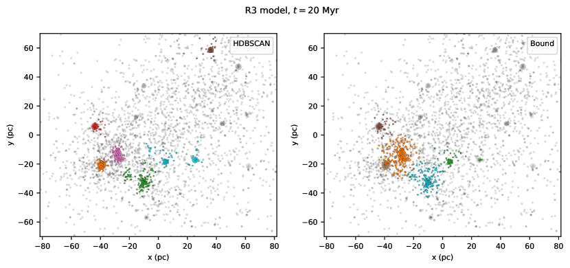
Figure 2: Groups identified at 20 Myr in model R3. The left panel shows groups identified using HDBSCAN, while the right panel shows bound systems (see §2.3). Each group is assigned a different color.

Table 2: Gas and star densities within the stellar half mass radius at the end of the STARFORGE simulations ($t_{\rm init}$).

Model	$\rho_{\rm gas,0}$	$\rho_{*,0}$	$R_{\rm*,h}$
	$M_{\sun}\,{\rm pc}^{-3}$	$M_{\sun}\,{\rm pc}^{-3}$	pc
fiducial	$1.45\pm 0.9\times 10^{-3}$	$0.2\pm 0.2$	$12\pm 4$
alpha1	$2.43\times 10^{-4}$	0.98	5.94
alpha4	$2.59\times 10^{-4}$	0.0222	16.1
R3	0.167	2.45	5.68
R30	$6.90\times 10^{-6}$	$1.73\times 10^{-3}$	23.9
Bx10	0.0135	0.139	11.0
Bx100	$5.72\times 10^{-3}$	0.0664	12.7
ISRFx10	0.0227	0.427	8.03
ISRFx100	0.0137	0.268	10.1
Z01	$8.41\times 10^{-3}$	0.0172	11.0
Z001	$3.23\times 10^{-4}$	0.0127	12.7

The STARFORGE simulations we adopt follow the star formation process of star clusters until star formation has mostly ceased. However, there is still a small amount of gas that is co-spatial with the stars. To quantify the significance of the remaining gas, we define the local stellar fraction (LSF) as the ratio of the total stellar mass to the total mass within the half mass radius of the stars: LSF$~{}=M_{\rm*,h}/(M_{\rm*,h}+M_{\rm gas,h})$. We find that in most models the LSF is above 90% (see Table 2). While we expect its impact to be small, in principle background residual gas could provide enough binding energy to affect the boundedness of the stellar groups. To determine if it is indeed a negligible factor, we perform a second series of simulations with a background gas representation. Since the hydrodynamical gas structure is complex and difficult to realistically describe in pure $N$-body simulations, we represent the gas gravitational potential using an approximate analytical distribution.

An analysis of the gas distribution indicates that, in most cases, a uniform distribution is a reasonable representation for the radial profile. We model a uniform distribution by adapting the Plummer sphere model implemented in Nbody6++GPU. This is modeled by adding the gravitational potential generated by a Plummer density distribution to the stellar potential:

$$\rho_{\rm pl}(r) =\rho_{c}\left(1+\dfrac{r^{2}}{R_{\rm pl}^{2}}\right)^{-\frac{5}{2}},$$ (3)

where $\rho_{c}$ is the central density and $R_{\rm pl}$ the scale radius. We choose a large $R_{\rm pl}$ such that the gas is uniform within the stellar half mass radius $R_{\rm*,h}$. The central density is the average density within the half mass radius of the stars. We show the values of the central densities in Table 2.

Since we expect stellar feedback from the stars to continue to disperse the remaining gas, we estimate the gas gravitational potential decay timescale by measuring the gas velocity dispersion inside the half mass radius of the stars. This depletion timescale is given by $\tau_{\rm M}=r_{\rm h}/\sigma_{\rm gas}$. We assume the gas mass of the Plummer sphere decays exponentially over this timescale as (Kroupa et al., 2001):

$$M_{\rm gas} =M_{\rm gas}(0)e^{-(t-t_{\rm D})/\tau_{\rm M}},$$ (4)

where $t_{\rm D}$ is a delay time for gas depletion that we set equal to zero, i.e. gas depletion begins at the start of the N-body calculation.

2.3 Stellar Analysis

2.3.1 Identifying Groups with HDBSCAN

Star formation simulations often form not only one but several stellar groups that move in different directions after formation (e.g., Kirk et al., 2014; Li et al., 2018). Paper IV found that many of the smaller groups merged during formation to become larger groups. In this work, we focus on the later evolution of the groups analyzed in Paper IV, and we study their kinematics, evolution and boundedness over the subsequent 200 Myr.

We identify groups in the simulation snapshots using the Hierarchical Density-Based Spatial Clustering of Applications with Noise (HDBSCAN) algorithm (Campello et al., 2013; McInnes et al., 2017; Malzer & Baum, 2020), implemented in Python. HDBSCAN is an extension of the DBSCAN algorithm (Ester et al., 1996) that adopts an adaptive rather than a fixed characteristic size for groups. Both methods have been previously used to identify stellar groups in surveys (see e.g., Castro-Ginard et al., 2018; Hunt & Reffert, 2021; Kerr et al., 2021; Tarricq et al., 2022).

The simplier DBSCAN algorithm works by identifying points that are “close" to each other according to some predefined distance metric, typically the Euclidean distance. DBSCAN requires two user-defined parameters: a characteristic minimum separation scale $\lambda$ and a minimum group size $N_{\rm min}$. A group is defined to be all stars located within a distance $\lambda$ of another star, where the total number of connected stars is at least $N_{\rm min}$. Stars that are not within $\lambda$ of any other stars or who are part of a group smaller than $N_{\rm min}$ are not assigned to any group.

DBSCAN works well for single snapshots and relatively well for time-series where the groups are of a similar size (although some extra measures are still needed to eliminate noise between time-series, see Paper IV, ). In our application, however, the expanding nature of the regions complicates the choice of $\lambda$. Groups from the same simulation may expand at different rates depending on whether they are more or less bound, and consequently, we need to find groups over a wide range of evolving densities. The HDBSCAN algorithm, which is a generalization of DBSCAN, addresses this specific problem.

The purpose of HDBSCAN is to find groups on a wide range of scales. Essentially, HDBSCAN analyzes all possible solutions of DBSCAN for a given value of $N_{\rm min}$, i.e., all possible choices of $\lambda$, and returns the groups that are the most persistent over a range of scales. HDBSCAN requires only two user parameters: $k$, which specifies the number of neighbors to consider when forming groups and $N_{\rm min}$, the minimum number of points in a group.

The HDBSCAN algorithm proceeds as follows: First, it uses the specified distance metric (Euclidean in our case) to find the distance to each star’s $k$-th nearest neighbour. This distance defines each star’s $k$-neighbour radius ${\cal R}_{k}$. Then, it uses the $k$-neighbour radius to define the mutual reachability distance metric, defined by:

$$d_{\rm reach}(a,b) =\max\{{\cal R}_{k}(a),{\cal R}_{k}(b),d(a,b)\}.$$ (5)

This definition provides robustness against outliers, so that sparsely distributed data, points with a large ${\cal R}_{k}$, are separated from the rest of the data by at least ${\cal R}_{k}$. This avoids the problem that a small number of data points may act as bridge between two well-separated groups.

Using $d_{\rm reach}$ as a metric, HDBSCAN creates a minimum spanning tree (MST) of the distribution, from which it constructs a hierarchical tree of connected points. It then walks the hierarchy by using different distance thresholds, from the large to the small scales, recording the groups that appear, split, and lose members as the $d_{\rm reach}$-threshold become smaller. The algorithm then evaluates which groups persist over different scales and selects the most stable groups (see Campello et al., 2013, for details on how stability is evaluated).

We use the same input parameters for all $N$-body simulations to select groups. We adopt a group size $N_{\rm min}=30$ and $k=5$ nearest neighbours to obtain ${\cal R}_{k}$. Note that HDBSCAN is equivalent to the DBSCAN algorithm, if instead of walking through the tree, we use a single $d_{\rm reach}$ threshold to obtain the groups.

2.3.2 Tracking Stellar Groups

Although we adopt the same fixed parameters for all simulations and snapshots, applying HDBSCAN still produces noisy results between some snapshots, i.e., the group membership fluctuates. This is because small variations in the stellar distribution can produce large variations in the assigned group membership. To address this issue, we down-sample the $N$-body simulation time outputs to 200 equally spaced times and apply HDBSCAN to the closest snapshot to each time.

Since groups may lose members, merge, split or disappear between successive snapshots we also develop an algorithm to match groups. Our algorithm builds and compares two lists of groups in consecutive snapshots. We call the first group, the one at the earlier time, the parent group and the one at the subsequent time is a child group. We match each list as follows:

1. We assign a name ${\cal N}_{i}$ to each parent.

2. We then compare each child group with each parent. If the child has any members of the parent ${\cal N}_{i}$, then we check if another child was already assigned to the parent.
   $\bullet$ If not, we give the child the parent’s name.
   $\bullet$ If the name was already assigned to another child, then we give the name to the one containing the most members and assign no parent to the smaller group (temporarily).

3. At the end of the list comparison, we assign a new name to all unassigned groups. These become potential new parents for the groups in future snapshots.

4. If a parent does not have any child group we keep its name and membership list for comparison in future snapshots. Occasionally, a group that disappears will reappear in a later snapshot.

However, even with this procedure, the group membership still fluctuates somewhat between snapshots as some groups undergo multiple splits and mergers while other groups are very short-lived and thus are irrelevant to our analysis. Therefore, in order to have well-defined time-stable groups we require an additional step to clean the group history. We use a similar method to Paper IV, by producing a “history” for each star, which we clean in the following way:

We follow the history of each star and identify instances where a star has been assigned to two or more groups within a characteristic time $t_{\rm clean}=5\,\rm Myr$.

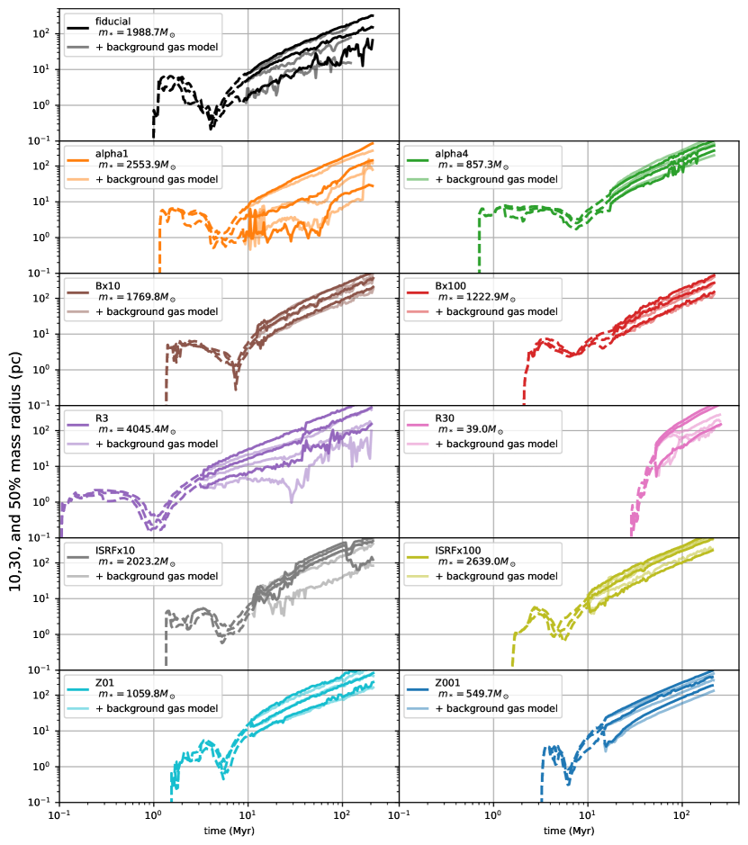
Figure 3: Evolution of region size expressed as the 10, 30 and 50% mass radius for each model. Dashed lines show the evolution during the STARFORGE simulation, while solid lines show the evolution in the $N$-body simulation. Bold solid lines represent models in the gas-free case (NoExtPot models), i.e., without any model for background gas. The semitransparent lines indicate the evolution including a background potential that represents residual gas (ExtPot models).

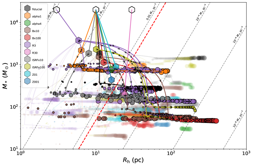
Figure 4: Stellar mass versus half-mass radius for systems formed in the STARFORGE  framework. Unfilled black hexagons show the parent cloud initial conditions, connected by a line to a colored filled hexagon that shows the state of the respective STARFORGE simulations when gas is expelled and the simulation ends. From there the $N$-body simulation begins, and we track the groups formed in each simulation. We show the state of the groups at each time, where the size of the circles is proportional to the cluster age. Semi-transparent points are groups identified by HDBSCAN, and black contour circles indicate the subset that are bound. Lines (with arrows for bound systems) show the average evolution of each identified bound group. Dashed lines indicate lines of constant mass density. Red dashed line represents the Jacobi radii at the position of the Sun.

The cleaning procedure is as follows:

1. We create a history of group membership for each star and examine the history for membership changes beginning at the last snapshot.

2. We give each star a single label for the last time span of size $t_{\rm clean}$, where the label represents the most frequent group assignment during this time.

3. We search each prior time for a membership change. If the star is not assigned to more than one group during the $t_{\rm clean}$ interval we call it a stable label. If this label represents a group, we call it a stable group label, i.e., a stable label can also indicate a isolated star, which is not assigned to any group. We use the stable group label to identify any large time-spans where a group was not identified by HDBSCAN. However, as the groups are expanding and there is little interaction between them, we find it useful to keep the group label identified during this time to provide continuity in the history. This allows us to track the group properties. Then, we assign the stable group label during any times of “missing” identification.

4. When a group assignment changes, there are three possible cases:
   Case 1) The new group label is the same as the last stable group assigned to the star. In this case, we label the star at times in between with the new label, ignoring the changes in between.
   Case 2) The new label is different and the old label was not stable, so we assign the last stable label to the time in between (either a group or no membership).
   Case 3) The label is different and the previous label is stable, then we keep the label during this time as if no change in membership had occurred.

5. If the last stable label assigned was a group, then we update the “stable group label“ and record its position.

6. We continue with this procedure until the first snapshot is reached. As a final step, we check the groups at every snapshot and remove any groups with less than 50 members.

2.3.3 Identifying stellar clusters

In addition to applying HDBSCAN, we post-process the resulting groups to identify their bound members. In a region with significant substructure, identifying bound systems is not trivial, as the final result depends on the frame of reference we use. For instance, two groups may be moving away from each other, such that selecting one of their center of mass velocities as the system velocity will make most of the other system members unbound. Also, measuring the center of mass of a system, ideally, would require considering only bound members, but the bound membership list is the information we are trying to obtain. To solve this circular problem, we use an iterative method that we refer to as “snowballing” (Smith et al., 2013b; Farias et al., 2015). After providing an initial position and radius ($r_{s}$), the method works in two steps:
1) An iterative process measures the bound members inside the starting radius. Using the center of mass velocity of stars inside $r_{s}$, we remove any unbound stars and correct the center of mass velocity. We repeat this step until it converges to a fixed number of bound stars.
2) With a robust bound region identified, we now consider all stars, adding any bound stars to the final sample. After correcting the center of mass velocity, we repeat this step until the solution converges, which is defined to be when no more than two stars change membership between steps or a maximum of 100 iterations is reached.

For the starting radius, $r_{s}$, and starting position, we use the groups selected by HDBSCAN, where $r_{s}$ is the minimum radius containing all stars and the starting position is the group center. HDBSCAN does not select stars that are too far from each group and therefore the effective size of the HDBSCAN group is a reasonable choice for $r_{s}$.

Figure 2 shows the groups identified with HDBSCAN (left) and the bound groups identified with algorithm described above (right) for model R3. Of the seven groups found with HDBSCAN, only two contain a significant number of bound members. Note that even though we use each of the HDBSCAN groups as a starting point to search for bound stars, some of these individual groups are bound and our method merges them together. Although we identify groups using HDBSCAN and adopt these groups as seeds for our cluster identification procedure, throughout this paper we analyze both sets of groups independently. The HDBSCAN groups represent how observers identify groups; sufficiently accurate kinematic information is not available in most cases to determine whether the groups are truely bound. The bound groups we identify using the second procedure represent true star clusters. The first set are useful to compare with and interpret observations, while the latter help us understand the physics behind star cluster formation.

3 Results

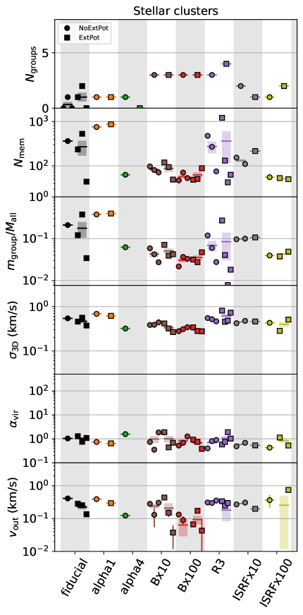
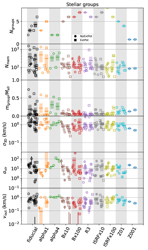
Figure 5: Time-averaged properties for groups of stars detected in each model between 8 to 12 Myr after the region’s expansion. Left panel shows the results for bound systems while left panels shows the results for systems found using HDBSCAN. Circles denote groups in models with no background gas (NoExtPot), while squares denote groups in models that account for background gas (ExtPot). Note that the fiducial set shows the results of three different runs. From top to bottom: the first panel shows the number of identified groups in each model, the second panel shows the number of members in each group, the third panel shows the mass of the groups relative to the total stellar mass, the fourth panel shows the 3D velocity dispersion of the stars, the fifth panel shows the virial parameter of each system, where $\alpha_{\rm vir}=1$ represents virial equilibrium, and the bottom panel shows the median expansion velocity from the center of each group.

3.1 Evolution and survival of star clusters

In this section we present the long-term evolution of the stars born in the STARFORGE simulations. We compare the evolution with and without a background potential that represents residual gas. Figure 3 shows the global evolution of the 10, 20 and 50% radius relative to center of mass of all stars in each simulation, where the STARFORGE evolution phase is denoted with dashed lines. The evolution of the young stars, modeled by STARFORGE, shows that star formation happens over a few to 10 million years. As collapse proceeds, the stars become more centrally condensed (in all but the R30 simulation) at which point stellar feedback is strong enough to stop star formation and disperse the gas. In all runs the stars and residual gas do not have enough gravity to confine all the stars; the global SFE is very low, and, consequently, the stellar complex expands. Therefore, each GMC produces the equivalent of an association complex. As previously shown in Paper IV, this includes a range of smaller groups. We analyze the behavior of the subgroups in §3.2.

We find the half mass radii of all regions expand monotonically, indicating that the systems are not bound at this scale. However, for the 30% and 10% mass radius, two stellar complexes show signs of dynamical evolution. Model alpha1  shows a relatively constant 30% mass radius for about 50 Myr, before starting to expand again. This is a sign that a considerably large bound system was formed (see §3.2). However, large formed star clusters do not always show a signature in the size evolution of the region. As we show below, one of the fiducial models produces a similar size star cluster, but the global evolution of the region still shows monotonic expansion.

In general, accounting for the residual gas does not greatly affect the behavior of the expanding regions. However, in some particular cases, adding a background potential triggers the capture of a considerable number of new members. In one extreme case in the R3 model, background gas triggers the capture of $\sim 500$ new members, by merging two big clusters (see below). This affects the overall size of the region as the most prominent clusters merge into one rather than separating apart. In another notable case, the alpha1 model forms a single cluster that is slightly more massive than in the R3 model. The addition of a background potential causes only a minor increase in the cluster’s mass. However, the evolution of the half-mass radius exhibits distinct oscillations over time between the two cases. This reflects ongoing dynamical evolution that is absent in other expanding regions with less massive clusters. These instances underscore the fact that the intrinsic chaotic nature of the N-body problem implies that the inclusion of a background potential, even one representing a small mass fraction, may trigger unexpected behaviors, particularly in substructured stellar regions.

3.2 Characterizing stellar groups

One important motivation of this work is to characterize the populations of star clusters that form in the STARFORGE calculations. However, there are two approaches we can take for this problem. One, is to characterize the groups of stars that observers would detect by using clustering algorithms such as HDBSCAN. The other approach is to use the full available information to characterize the true bound systems that form in each model. Both approaches provides useful insights into the star cluster formation process, and therefore we will present both.

Figure 4 presents an overview of the identified clusters and groups and their mass-size evolution. This diagram illustrates that, in general, groups and clusters initially expand without losing a significant number of members. We also include the Jacobi radii at the Solar position as a reference, and we observe that most groups fill these radii with their half-mass radii soon after formation. This suggests that most of these groups would be stripped out in a galactic environment shortly after formation. Therefore, our analysis is primarily constrained to the first 10 million years after their expansion begins.

3.2.1 Groups sizes and frequencies

Figure 5 shows a comparison of different parameters for each group averaged over a narrow time-span after the expansion of the region, early enough for the regions to be young and late enough for the groups to be well separated, i.e., we choose to average the properties between 8 to 12 Myr after the expansion of the region begins. The left panel shows the results for bound systems, while the right panel shows groups identified with HDBSCAN. Squares indicate the models that represent residual gas using a background potential, the ExtPot case, while circles indicate models that neglect residual gas, the NoExtPot case. Note that the cases with and without background gas are statistically similar in all cases, although there are slightly more massive systems in the ExtPot case.

While HDBSCAN identifies on the order of 2 to 8 groups in each simulation, we see that a smaller number are identified as (bound) clusters. The largest numbers of clusters are found in the strong magnetic field models Bx10, Bx100 and the high-surface density model R3, which each have three to four bound systems. However, the clusters in the stronger magnetic field models are relatively small and contain less than a hundred members each, which is smaller than the typical cluster size in the fiducial case. These small clusters do not affect the half mass radius of the stellar complex (see Figure 3), as they contain less than 10% of all the stars and are moving away from each other. The stronger magnetic field induces the formation of a larger number of bound systems, but their total mass is still less than the total cluster mass in the fiducial case and, as we will see below, most of them are short lived.

The largest star clusters are found in the R3 model where the size of the clusters varies strongly with the addition of background gas. In the ExtPot case, the largest cluster contains $\sim$1100 members. It is accompanied by three smaller clusters with $\sim$30, 50 and 100 members. In the NoExtPot case the largest clusters have $\sim 500$ and $\sim 200$ members. The big difference in membership between the ExtPot and NoExtPot models is caused by the merging of the two larger star clusters formed in the R3 model. The mass of both clusters together triggers the capture of additional members increasing the difference between the ExtPot and NoExtPot cases. The bigger cluster contains about 28% (see below) of the stars in the simulation and triggers a different evolution in the 30% radius of the region as we discuss above.

The next largest cluster is formed in the alpha1 case, which has a single cluster with $\sim 800$ and $\sim$900 members in the NoExtPot and ExtPot cases, respectively. The higher turbulent velocity case, alpha4, produces one ($\sim 60$ members) or zero bound systems.

In the low-density cloud model, R30, no clusters or groups were identified due to the limited number of stars formed and their dispersed distribution within the simulation. Compared to the formation event, specifically the gas expulsion timescale (see § 3.4.2), the dynamical timescale of the region is relatively long, which hampers any interactions between stars or adjustments of their orbits to the relatively rapid decrease in the region’s gravitational potential.

The third row of panels in Figure 5 shows the fraction of stellar mass in each group relative to the total stellar mass. For individual star clusters this represents their bound fractions, while the total mass in star clusters represents the total bound fraction of the stellar complex, which we discuss in § 3.4.2. Only the fiducial, R3, and alpha1 models form star clusters containing more than 10% the stars in the region. The alpha1 model has the highest individual bound fraction, $\sim 40\%$, by a slim margin.

The right panel of Figure 5 shows that HDBSCAN identifies more groups and that these groups are in general bigger than the identified clusters, as energy constraints are not taken into account. The fiducial  and alpha1 cases have the largest groups with more than 1000 members. HDBSCAN finds some small unbound groups in the models with lower metallicity, which formed no clusters. This indicates that these runs still contain substructure, although all the groups are smaller than 300 members with less than 100 members total in the Z001 case. Lower metallicity also makes it more challenging to form groups: fewer stars form overall because the increased HII region temeperature and reduced recombination greatly increases the rate of HII region expantion.

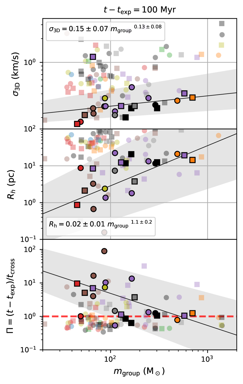
Figure 6: Kinematic parameters for stellar clusters (solid symbols) and groups (semi-transparent symbols) as a function of $m_{\rm group}$. Values are measured at 10 Myr (left panel) and at 100 Myr (right pannel) after the region expansion. Circles and squares show the NoExtPot and ExtPot cases, respectively. Top panels display the three-dimensional velocity dispersion, $\sigma_{\rm 3D}$, middle panels show the group half mass radius $R_{\rm h}$, and bottom panel show their dynamical age, $\Pi$. Bound cluster size and velocity dispersion correlate with group mass according to the fit equations shown in the respective panels. The solid lines in the bottom panel show the above relations applied to the dynamical time. The red dashed lines $\Pi=1$, which has been proposed as a threshold between star clusters and associations (Gieles & Portegies Zwart, 2011).

3.2.2 Dynamical state and scaling relations

The fourth row of panels in Figure 5 shows the three dimensional velocity dispersion of the clusters and groups, $\sigma_{\rm 3D}$. We remove orbital motion from the velocity dispersion by adopting the center of mass velocity for binary pairs; consequently, the dispersion provides a direct measure of the internal dynamics. Interestingly, all star clusters have a similar velocity dispersion that is independent of the parent cloud properties. The cluster velocity dispersions range from 0.2 to 0.8 $\rm km\,s^{-1}$, which is well below the bulk simulation gas velocity dispersion. Although the HDBSCAN group velocity dispersions are higher (0.2-20 $\rm km\,s^{-1}$), they also do not appear to correlate with the parent cloud kinematics.

We obtain a similar result when measuring the group virial parameter (see fifth row of panels). By construction all star clusters have $\alpha_{\rm vir}\sim 1$, while the HDBSCAN groups span a wider range with $\alpha_{\rm vir}\sim 1-100$. This suggests that many observed young groups identified by proximity rather than kinematics may be significantly unbound.

While we find no correlation between the cloud initial conditions and the dynamical state of the groups, we do find a scaling relation between velocity dispersion, cluster size and the stellar group mass, $m_{\rm group}$, as illustrated in Figure 6. The top panel shows a tight scaling relation between velocity dispersion and cluster mass. Using the least squares method, we fit a power law to the clusters at 10 Myr after the cluster expansion ($t_{\rm exp}$, see last column of Table 1), resulting in the relation $\sigma_{\rm 3D}\propto m_{\rm group}^{0.21\pm 0.02}$. We find a similar power law exponent at 100 Myr, $0.13\pm 0.08$ (see the right panel of Figure 6). Note that in general, we do not expect the power law index to remain static over time, because the velocities of bound systems change due to the evolution of the multiple systems, the ejection of members, and stars adapting to the expansion of the cluster. However, as the clusters analyzed here are relatively small and undergo relatively little additional relaxation, the relationship between group mass and velocity dispersion does not vary much.

The middle panels of Figure 6 show a broader correlation between cluster mass and radius, where $R_{\rm h}\propto m_{\rm group}^{0.4\pm 0.1}$. This relation varies significantly with time, such that the power law index rises to a value of $1.0\pm 0.1$ at 100 Myr. These correlations arise as a consequence of the narrow velocity dispersion mass relation. Since star clusters are bound, their velocity dispersion, mass, and radius are related through the virial parameter as follows:

$$\alpha_{\rm vir}=\frac{2E_{\rm kin}}{E_{\rm pot}}=\frac{1}{2}\frac{\sigma_{\rm 3D}^{2}R_{\rm h}}{\eta Gm_{\rm group}},$$ (6)

where $E_{\rm kin}$ and $E_{\rm{\rm pot}}$ are the kinetic and potential energy of the stars respectively, $G$ is the gravitational constant, and $\eta$ is a profile-dependent constant for the potential of the distribution of stars. Using the half-mass radius as the scale radius, for a Plummer sphere, this value is $\eta=0.13$. Then, based on the $\sigma_{\rm 3d}$-$m_{\rm group}$ relation above, we would expect $R_{\rm h}\propto m_{\rm group}^{0.58}$ and $R_{\rm h}\propto m_{\rm group}^{0.9}$ at 10 Myr and 100 Myr, respectively. These values are very close to the power law fits over-plotted in the middle panels of Figure 6, where variations are due to the structure and different expansion rates of the individual clusters.

One way to assess the rate at which star clusters expand, and consequently their stability over time, is to compare their age to their current crossing time. This ratio between age and crossing time is termed the dynamical age ($\Pi$). Systems that undergo rapid expansion exhibit low values of $\Pi$, which decrease as time progresses. In contrast, stable systems show an increasing dynamical age, reflecting relatively constant crossing times over time. Applying the relationships mentioned earlier, we observe a shift in the correlation of cluster crossing times over time. Initially, at 10 Myr, clusters of all masses follow a rather uniform crossing time, with a correlation of $m_{\rm group}^{0.2}$. However, this correlation becomes more pronounced and linear by 100 Myr, highlighting that more massive clusters expand faster than smaller clusters.

The bottom panels of Figure 6 show $\Pi$ at 10 and 100 Myr, where we adopt the time since expansion ($t-t_{\rm exp}$) as the cluster age. Gieles & Portegies Zwart (2011) proposed a value of $\Pi=1$ as a threshold to distinguish between star clusters and associations. We observe that larger clusters sustain a value of $\Pi$ close to unity for over 100 Myr. In contrast, smaller clusters, which do not expand as rapidly, increase their dynamical age values over time, rising from $\lesssim 1$ to values closer to 10 at 100 Myr. However, as these systems are small and their dynamical timescale is short, at 100 Myr about 40% of clusters with masses below 100 $M_{\sun}$ dissolve. For clusters with masses above 100 $M_{\sun}$, this figure drops to 10% of dissolved clusters.

This result shows that small clusters, while able to form stable systems, can sustain their increasing densities for only a short period. Larger clusters form stable configurations, but dynamical interactions, rather than dissolving them, cause a constant expansion.

Stellar groups follow similar trends to those of the clusters but exhibit significantly more scatter. Like the clusters, their properties do not correlate with initial cloud properties, and groups formed within super-virial clouds are not different in radius or velocity from ones formed in sub-virial clouds. However, high-velocity stars cause most stellar groups to scatter above the mass-velocity dispersion relation for star clusters. In the mass vs. half-mass radius diagrams, the groups tend to lie above the relationship observed for clusters. This is mainly due to the fact that HDBSCAN groups typically consist of a larger number of members that are more sparsely distributed across larger volumes. However, this is not always the case.

The dispersion in velocity and high-mass radius exhibited by the stellar groups produces significant scatter in the dynamical age vs. mass diagram. Although, the majority of groups show dynamical ages below 1 at all times, a significant fraction of them scattered above this threshold. This variation is more prominent for groups with masses $\lesssim$100 $M_{\sun}$in particular. Above this threshold, groups and clusters exhibit similar trends, possibly attributed to the fact that groups encompass bound clusters. Given their larger size, a greater proportion of group members are bound.

In the regime explored in this work, for clusters ranging from 30 $M_{\sun}$to 1000 $M_{\sun}$, higher mass clusters expand more rapidly than lower mass clusters. It remains uncertain to what extent these findings extend to larger systems, as the increase in cluster mass might mitigate the dynamically induced expansion due to the deeper gravitational potential. Nevertheless, these results imply that the stability of newly formed star clusters is predominantly determined by their mass rather than their initial conditions.

3.3 Group evolution and kinematics

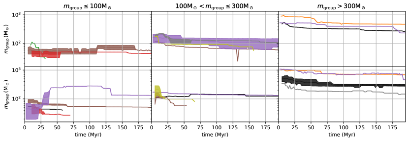
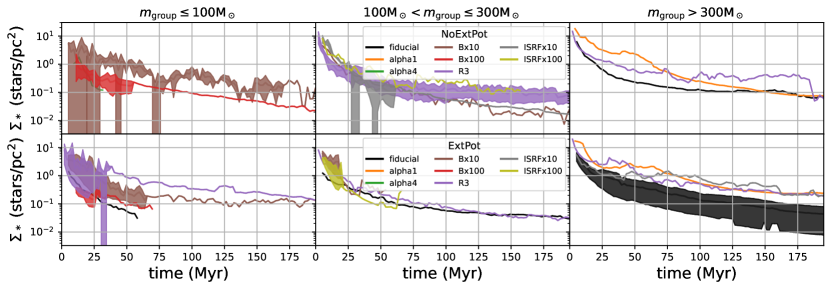
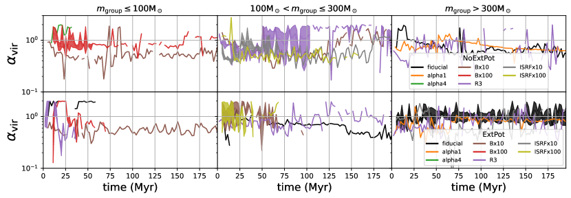
Figure 7: Evolution of different parameters grouped by mass range for identified star clusters. From top to bottom: evolution of the cluster mass ($m_{\rm group}$); cluster surface density ($\Sigma_{*}$) versus time; virial parameter ($\alpha_{\rm vir}$) versus time. In each set of six panels, the bottom and top rows show simulations with (ExtPot) and without (NoExtPot) residual gas, respectively. Each line shows the average value for the groups formed from the same parent cloud for the given mass range. The shaded areas show the standard deviation from the average; lines with no shading represent a single group.

The clouds analyzed in this work, which have a total initial mass of $2\times 10^{4}\,M_{\sun}$, form groups of stars with masses from $\sim 20\,M_{\sun}$ to $\sim 1000\,M_{\sun}$. To further investigate mass-dependent evolutionary trends, we group these systems into three mass ranges, where small groups have $m_{\rm group}\leq 100\,M_{\sun}$, medium groups have $100\,M_{\sun}<m_{\rm group}\leq 300\,M_{\sun}$ and big groups have $m_{\rm group}\geq 300\,M_{\sun}$. Although the group mass evolves as the membership changes, we adopt $t=10$ Myr after the expansion begins to characterize the mass of the systems (as we did for Figure 5).

Figure 7 shows the evolution of each cluster’s mass, two dimensional stellar surface density ($\Sigma_{*}$) within each cluster’s half-mass radius, and stellar virial parameter. The lines indicate averages for clusters formed from the same cloud and in the same mass range, while the shaded areas show the standard deviation from the mean; single lines represent a single surviving cluster. About 40% of small star clusters dissolve before 70 Myr due to their low mass and shorter crossing times, making them susceptible to dynamical evaporation. However, around half of them manage to survive for up to 200 Myr. With increasing cluster mass, their longevity improves, a result attributed to the mass-dependent cluster expansion discussed in §3.2.2. Larger clusters primarily experience mass loss during their early stages when densities are higher. As these clusters expand, their crossing times increase, reducing the occurrence of dynamical interactions that could lead to evaporation.

The middle panels of Figure 7 show that the stellar half-mass surface density, $\Sigma_{*}$, declines during the first $\sim$100 Myr for all clusters. A few clusters, namely one small cluster in model Bx10, a large cluster in the fiducial model and a couple intermediate-sized clusters in model R3, reach a steady-state surface density of $\Sigma_{*}\sim 10^{-1}$ stars/pc², indicating that expansion has halted. As discussed in §3.2.2, high-mass clusters exhibit more prominent density changes during the initial 100 Myr. By examining the stellar surface densities, we note that low-mass clusters experience a slower decrease during this time compared to higher-mass clusters that exhibit a rapid initial decline in density. The overall evolution and final cluster surface densities appear to be largely insensitive to the initial gas conditions, however. Similarly, the presence of residual gas seems to have little effect on the final surface densities.

One prevailing trend is that the virial parameter remains relatively constant over time. As the star clusters expand, there is minimal dynamical evolution observed. We do not identify clear relationships between mass and $\alpha_{\rm vir}$. Notably, significant fluctuations in the virial parameter overlap across different clusters. These variations result from factors such as the precise selection of members, accurate identification of binary and multiple systems, and the chosen reference frame for kinetic energy measurement. Slight discrepancies between two consecutive snapshots could lead to significant alterations in the virial parameter value, particularly when dealing with a small number of members.

3.4 Star cluster birth environment

In the classical picture of star cluster formation, the fraction of mass that remains bound after gas removal depends on the global SFE and also the timescale on which such gas leave the region. High SFE and long gas expulsion timescales offer the most favorable conditions to form bound clusters (e.g. Baumgardt & Kroupa, 2007; Smith et al., 2013a). This dependence has been studied mainly by the use of pure $N$-body simulations with spherically symmetric background potentials to mimic the influence of the gas. Although in this work we also make use of such potentials, we do so at the later stages of gas expulsion where the potential generally represents only a few percent of the mass and its contribution to the evolution of the cluster is minor. The bound clusters studied here are the result of the complex interactions between stars and gas, each with their own substructures.

The STARFORGE simulations provide a unique opportunity to study the early dynamics between gas and stars in a realistic setup, which can be compared with the classical picture of star cluster formation. In this section we investigate how the primordial kinematics of stars within the parent cloud and the cloud evolution affect the structure and survival of star clusters.

3.4.1 Gas expulsion timescale

Table 3: Estimated gas expulsion timescales and fit parameters. The first four columns indicate the model name, estimated gas expulsion timescale $\tau_{\rm exp}$, decay time $t_{\rm D}$, and fit time-range, beginning at the time when gas mass starts to decline $t_{\rm D}$. The fifth column assess the quality of the fit using the ${\cal R}^{2}$ test, and the last column shows the estimated gas expulsion timescale normalized by the cloud initial free fall time.

Model	$\tau_{\rm exp}$	$t_{\rm D}$	$t_{\rm max}$	${\cal R}^{2}$	$\tau_{\rm exp}/t_{\rm ff}$
	[Myr]	[Myr]	[Myr]
fiducial	$1.7\pm 0.1$	2.53	9.50	0.90	$0.48\pm 0.03$
alpha1	$1.4\pm 0.1$	2.78	7.50	0.90	$1.05\pm 0.05$
alpha4	$3.9\pm 0.2$	1.26	14.8	0.96	$0.39\pm 0.03$
R3	$0.55\pm 0.02$	0.249	2.50	0.94	$0.90\pm 0.04$
R30	$1.73\pm 0.09$	38.7	51.1	0.79	$0.090\pm 0.005$
Bx10	$2.6\pm 0.2$	2.27	11.5	0.91	$0.72\pm 0.04$
Bx100	$2.4\pm 0.5$	3.66	7.60	0.95	$0.6\pm 0.1$
ISRFx10	$2.4\pm 0.2$	3.16	10.5	0.89	$0.64\pm 0.05$
ISRFx100	$1.6\pm 0.1$	3.16	8.90	0.94	$0.44\pm 0.03$
Z01	$1.43\pm 0.06$	3.66	10.8	0.49	$0.38\pm 0.02$
Z001	$0.79\pm 0.06$	4.79	8.21	0.84	$0.21\pm 0.02$

One important parameter that has remained largely unconstrained in $N$-body studies is the gas depletion timescale, $\tau_{\rm M}$. Its critical importance comes from the fact that star cluster formation is inefficient. As star clusters transition from their embedded stage into a gas-free phase, most of the gravitational energy binding the cluster together vanishes with the gas. If the transition happens rapidly, quicker than a crossing time, stars do not have sufficient time to adapt their orbits to the new potential, and a large fraction of them suddenly find themselves unbound. Previous studies have left $\tau_{\rm M}$ as a free parameter or used an arbitrary value. Here we measure this parameter directly from the STARFORGE simulations, setting theoretical constraints for gas expulsion timescales.

As shown in Sec. 2.2.4, we adopt an exponential decay functional form to model the expulsion of residual gas from the cluster, which is the standard practice in the $N$-body literature. However, $>90\%$ of the gas is cleared out of the system by radiation and winds before the first supernovae occurs (Paper IV) and before we begin the $N$-body modeling. We refer to this gas removal timescale as dispersal time. Therefore, it is possible to calculate the dispersal time, which governs most of the gas dispersal, directly from the STARFORGE calculation, which we do here. We refer to this self-consistent dispersal timescale as $\tau_{\rm exp}$, which is different than the one we use in the $N$-body modeling, $\tau_{M}$, to describe the removal of the remaining residual gas.

To estimate $\tau_{\rm exp}$, we first measure the gaseous mass enclosed inside the 50, 80 and 90% radius of the stellar component. Then, we fit the exponential decay model described by Equation 4 using a least squares method. In this procedure, we fit $\tau_{\rm exp}$ as the single free parameter. We select the scale mass $M_{\rm gas,0}$ and delay time $t_{\rm D}$ based on the time when the enclosed gas mass reaches a maximum. Note that we use the gas mass enclosed by the stars, so the point where the maximum gas is enclosed depends on the forming stellar distribution and is by definition less than the total cloud mass. We fit Equation 4 to the range between $t_{\rm D}$ and the time just before the explosion of the first supernova, at which point the remaining enclosed gas mass declines sharply. Figure 8 shows this fitting procedure applied to the fiducial simulation.

We report the resulting fit parameters for the gas enclosed within the half mass radius of the stars in Table 3 and compare the result to the initial free fall time of the cloud. We assess the goodness of the fit using the ${\cal R}^{2}$ test, which compares the fitting function residuals to the residuals obtained by using a data average over the fitting range. We find that the exponential decay model in Equation 4 is, in general, a good description of the gas removal that occurs due to radiation and wind feedback. This is corroborated by the high ${\cal R}^{2}$ values, considering only one degree of freedom is given to the fit. However, in some cases the erratic evolution of the enclosed gas precludes a good fit, such as the case of Z01, which has ${\cal R}^{2}=0.49$. The goodness of fit depends on the location of the star cluster center with respect to the gas, as well the relative size of both components. Cases such as the Z01 model, where stars expand faster than the gas for a period of time, or instances where the stars move through overdense regions compromise the goodness of the description.

Normalizing by the initial free-fall time of the cloud indicates an order of magnitude spread in the characteristic timescale. The alpha4 model, where $\tau_{\rm exp}/t_{\rm ff}=1.05\pm 0.05$, has the longest relative gas-depletion time. This model has a long formation time such that the star cluster maintains a relatively constant size (see Figure 3). The stellar distribution in this model takes longer to contract, as the orbits are more energetic, and it takes more time for the gas to be cleared from a larger volume. The R30 model is at the opposite extreme; its depletion timescale is less than 10% of its free fall time. However, the relatively short depletion timescale explains why this model forms no bound systems (see Fig. 5). Models with stronger external radiation fields and lower dust abundance, i.e., those with warmer gas temperatures and more efficient stellar feedback, also show short depletion timescales as we would expect.

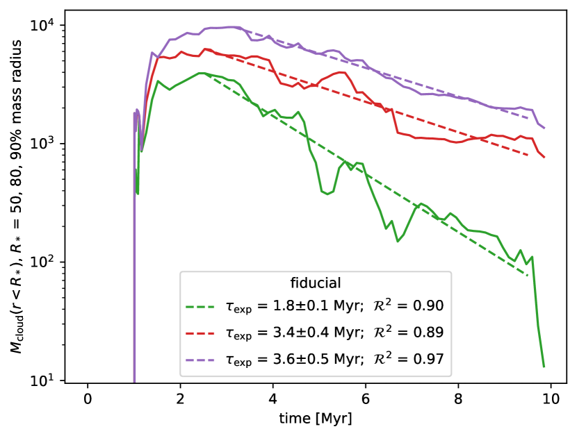
Figure 8: Gas mass enclosed within the 10, 50, 80 and 90% stellar mass radius during the fiducial STARFORGE simulation. Dashed lines shows the standard exponential decay timescale fit to the gas evolution.

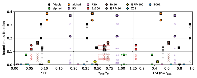
Figure 9: Total bound fraction as a function of global SFE (left), and gas expulsion timescale $\tau_{\rm exp}$ normalized by the cloud initial freefall time (middle) local, stellar fraction (LSF) at the moment of cluster expansion (right). Filled circles and squares show global bound fractions for NoExtPot and ExtPot  simulations, respectively. Analogously, semitransparent dots and crosses show bound fractions for individual clusters.

3.4.2 Bound fractions

As shown above, the simulated clouds often form more than one bound star cluster and these are generally a subset of the stars identified in stellar groups. In this context, we define bound stars as stars that are part of any of the identified clusters within a given simulation. Then, the total bound (mass) fraction refers to the ratio between the total number (mass) of bound stars in a model relative to all stars formed in that simulation. We use the term individual bound fraction to compare one cluster to the total mass or number of stars in its parent region.

Figure 9 compares the total bound fractions obtained 10 Myr after the expansion with the global SFE, LSF measured at $t_{\rm exp}$, and explusion timescale $\tau_{\rm exp}$. We observe a strong correlation between the bound fraction and the global SFE. Interestingly, within the range of SFE values obtained from the STARFORGE simulations (i.e. SFE$<0.2$), classical models do not predict the formation of any bound systems in the instantaneous gas expulsion limit. Here, more gradual gas expulsion likely facilitates cluster formation at lower SFE. Previous numerical studies have also demonstrated that substructure in the stellar distribution increases the likelihood of forming bound systems in low SFE environments (see e.g., Smith et al., 2013a; Farias et al., 2015). The middle panel of Fig. 9, however, reveals that the bound fraction increases roughly linearly with normalized $\tau_{\rm exp}$, in agreement with classical predictions. However, three models notably deviate from the relationship: the alpha1, alpha4, and one of the fiducial runs.

The alpha1 and alpha4 models suggest that the turbulent velocities and degree of boundedness of the parent cloud significantly influence the bound fraction. The alpha1 simulation yields the highest bound fraction among all models, despite having a relatively low SFE (0.07) and rapid gas expulsion compared to the cloud’s free-fall time ($\tau_{\rm exp}/t_{\rm ff}=0.38$). In contrast, the alpha4 model has both a low bound fraction and a low SFE, but its expulsion timescale is the longest among the models. Consequently, its position in Figure 9 lies below the other models. It is conceivable that these two models follow distinct relations between bound fraction, SFE, LSF, and $\tau_{\rm exp}/t_{\rm ff}$. The case of the outlier fiducial run, however, underscores that star cluster formation is a stochastic process and that other factors may come into play.

Previous numerical studies (e.g., Goodwin, 2009; Smith et al., 2011; Smith et al., 2013a; Farias et al., 2015) have argued that parameters such as the LSF and the virial parameter at the moment of gas expulsion yield improved estimates of the post-gas-expulsion bound fraction compared to the global SFE. However, the gas expulsion process, as discussed in §3.4.1, occurs over a prolonged timescale that begins early in the star formation process. Hence, the exact moment of gas expulsion is ambiguous. It’s important to note that by the time gas expulsion is considered to “begin,” less than half of all stars have actually formed. An alternative reference point could be the onset of expansion ($t_{\rm exp}$) of the stellar region. At this point, stars have undergone significant dynamical relaxation, and it is likely that the majority of the dynamical interactions that stars will experience have already occurred.

The last panel in Fig. 9 shows that LSF measured at $t_{\rm exp}$ also imperfectly correlates with the bound fraction. In this case, the outlier fiducial  in the previous panels has the highest LSF of all the models at $t=t_{\rm exp}$. However, it is worth noting that the bound fractions obtained for clusters with high LSFs are significantly lower than those found in $N$-body experiments, which assume instantaneous gas expulsion (see e.g. Farias et al., 2015; Farias et al., 2018).

On the other hand, we observe no correlation between the virial parameter of the stars and the bound fraction for either gas expulsion definition. This lack of correlation may be due to the longer timescales over which gas expulsion occurs. The virial parameter exhibits significant variations during the cluster’s formation (see Figure 7), and there is no single point in time that can accurately represent the cluster’s overall dynamical state.

Altogether, these results imply that the virial state of the parent cloud, along with the SFE and gas expulsion timescale, plays a crucial role in the formation of bound clusters.

3.4.3 Primordial kinematics

Despite a diverse set of initial conditions, we find that the cluster kinematic properties, particularly the velocity dispersions, are remarkably similar only 10 Myr after the expansion of the stellar complex begins. This raises the question: do star clusters inherit kinematic properties of the parent cloud or do they form with independent velocity signatures? To address this question, we trace back bound members from the identified star clusters and examine their velocity dispersion histories and places of birth. Figure 10 displays the evolution of $\sigma_{\rm 3D}$ for the fiducial, alpha1, and R3 models.

Figure 10 shows that stars destined to form bound clusters are born with slightly lower velocity dispersions compared to other stars. The initial velocities of the stars are correlated with the parent cloud velocity dispersion. For the fiducial, alpha1, and R3 cases shown in the figure, the initial cloud velocity dispersions are 3.2 $\rm km\,s^{-1}$, 2.3 $\rm km\,s^{-1}$, and 5.8 $\rm km\,s^{-1}$, respectively (see Paper IV, ), while the early stellar velocity dispersion is about a factor of 2 lower. However, the stellar dispersion quickly increases as the stars become centrally condensed, exceeding the initial cloud dispersion and reaching a constant value. The kinematics of bound members remain coupled to the rest of the region until shortly after the complex begins to expand, although their velocity dispersions are generally smaller than the global stellar dispersion.

Consequently, we conclude the similar velocity dispersions among the bound systems after expansion are partly due to a selection effect. During the violent relaxation that occurs during the region’s contraction, the least energetic stars tend to remain together, effectively erasing any signature of their parent cloud’s velocity dispersion.

Traceback of the individual members of the identified star clusters demonstrates that the final bound members do not necessarily originate from the same local region within the cloud. The bottom panels of Figure 10 illustrate the distribution of bound members in model R3 at times close to their formation (0.5 Myr), when the stars are most centrally condensed (1 Myr), and at a later time when the bound clusters are fully formed and distinct (10 Myr). At early times the stars appear well-mixed, and there is no clear signature of their later cluster assignment. This indicates that bound clusters emerge from the dynamical relaxation and energy exchange between stars, wherein the least energetic stars come together in one or more clusters while the most energetic stars expand. This relaxation process erases any lingering kinematic signature of the parent cloud.

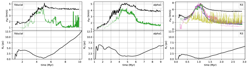
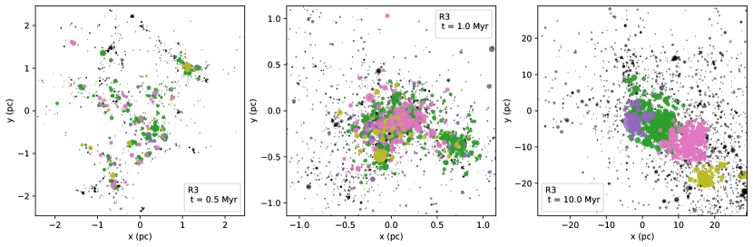
Figure 10: Top: Velocity dispersion for three STARFORGE models as a function of time for all stars (black solid lines) and for members of bound clusters found at 20 Myr after the expansion of the region shown in different colors. To calculate the velocity dispersion we use the center of mass velocities of binaries and higher-order multiples. Bottom: Position of bound members at 0.5, 1 and 10 Myr for the R3 case. Colors in the bottom panels match the groups in the top R3 panel.

4 Discussion

4.1 Clusters versus associations

The STARFORGE framework has provided a more self-consistent star cluster formation model than has previously been available, resolving individual stars and include all key feedback mechanisms. These processes are crucial for understanding the early dynamical state of young stellar groups and the process by which star clusters transition from embedded to gas-free entities. We find that in general the STARFORGE simulations form expanding stellar complexes that contain smaller bound clusters and unbound associations on a range of scales. Given the low global SFE in the simulations, the total bound mass contained in all modeled stellar complexes is below 1000 $M_{\sun}$, $<40\%$ of total stellar mass, with an average of 20%; this is either contained in a single cluster or spread between several sub-clusters. Unbound associations, which may be a mixture of bound and unbound stars, naturally contain larger mass fractions compared to the total mass or between 20% and 80% all stars in the complex. Given that our models do not account for tidal disruption from the host galaxy or nearby GMCs, which would decrease the fraction of surviving clusters, our mass fractions represent upper limits (Kruijssen et al., 2012; Kruijssen, 2012).

Our main takeaway is that, while most star systems form with a high degree of clustering, these systems primarily form in (unbound) associations not (bound) clusters. The detailed kinematics available from the STARFORGE simulations underscore that most stars are not born into clusters, at least in the galactic conditions that we have modeled. This conclusion is consistent with recent Gaia observations, which have provided a wealth of kinematic data of young stellar complexes, thereby allowing a clear distinction to be made between clusters and associations (Chevance et al., 2022). Debate on the topic of cluster vs. association has been muddied over the years by different definitions of what constitutes a star “cluster," a term that has historically depended on some predefined separation scale and/or stellar density (e.g., Lada & Lada, 2003; Gutermuth et al., 2009). The significant differences we find between stellar groups, defined using spatial information, and clusters, identified using full kinematic information, underscore the challenges of observationally identifying young clusters and predicting their evolutionary outcomes without accurate spatial and kinematic information.

4.2 Implications for massive cluster formation

We demonstrate in this study that clusters are formed with a range of masses and densities, and their kinematic properties depend more on their individual masses than the initial conditions of their parent cloud (see below). By extrapolating trends shown in Fig. 6, we anticipate that denser and/or more-massive clouds than those considered are needed to produce more massive and long-lived clusters. This has been found in previous, lower-resolution GMC and galaxy simulations accounting for stellar feedback (Li et al., 2019; Grudić et al., 2021b), but this regime still warrants exploration with a more self-consistent numerical treatment of star formation.

However, there are also secondary effects that influence the final cluster mass. As shown in Fig. 9 higher SFE indeed correlates with the formation of higher-mass clusters. SFE in turn correlates with high-surface densities and lower initial gas velocity dispersions. Some amount of residual gas, at the few percent level, also boosts the final cluster mass. This suggests there are multiple variables that interact to promote the formation of high-mass clusters. Additional simulations of clouds with realistic feedback processes are necessary to fully explore the parameter dependencies and investigate the more extreme conditions likely required to form massive clusters.

4.3 Group Selection

In contrast to some recent observational studies (e.g. Hunt & Reffert, 2021; Kerr et al., 2021; Quintana et al., 2023) we do not use velocity information to identify groups. We find that using velocities for group identification produces much noisier groupings, which experience more membership changes over time. For example, if a group contains binaries and higher order multiples, these members are often rejected from the selection because of their orbital velocity.

Observationally, it is advantageous to use velocities for selection as it helps to eliminate field stars that have large velocity differences with the groups of interest. In addition, most close binaries in the observed sample are not resolved, and thus populate a long tail in the observed stellar velocity distribution (e.g., Da Rio et al., 2017). However, in our case the system velocities are fairly similar and all our stars naturally form within the same cloud complex. We also have perfect identification of binaries, allowing us to correct for their velocities during the group and cluster identification process. Consequently, in our case the primary velocity differences come from the birth expansion rather than from different galactic orbits.

In cases where clustering algorithms employ velocity information, our analysis suggests that the orbital velocities of unresolved binaries cause the exclusion of cluster members and modify the appearance of any sub-structure. The absence of complete kinematic information and the ability to correct for orbital motion, likely causes weakly bound clusters to be identified as associations, particularly those with low membership and low stellar density.

4.4 Dynamical dependence on group mass

Our stellar groups span two orders of magnitude in mass, thereby allowing us to investigate variation in group properties as a function of mass. Notably, we observe that low mass clusters expand less rapidly during the first 100 Myr of evolution (see Figure 7), however a considerably fraction of them dissolve during this time. More massive clusters expand more rapidly initially, driven by dynamical interactions. However, after about 100 Myr, most of them are relaxed and reach a relatively steady stellar surface density of $\sim 0.05-0.1$ stars pc^-2.

We have shown that a ratio of age to crossing time, i.e., the dynamical age $\Pi$, of unity is consistent with the separation between bound systems and unbound groups, as proposed by (Gieles & Portegies Zwart, 2011). However, this distinction becomes noticeable only as stellar groups age. Shortly after the expansion of the complexes, at 10 Myr, both groups and clusters have dynamical ages below or close to unity. Low-mass clusters exhibit a rapid increase in dynamical age, while more massive clusters do so more gradually. By 100 Myr, they barely surpass this threshold. These results highlight the difficulty to assess the boundness of young expanding star clusters as, while they are bound, they do expand rapidly at shorter ages.

The emergence of these trends can be attributed to the remarkably consistent velocity dispersion of the identified groups. This produces a mass dependence, as groups of varying masses experience distinct relaxation patterns within this confined velocity range. Despite initial variations in the bulk gas velocity dispersion by a factor of three, the stellar velocity dispersions of groups identified by HDBSCAN after 10 Myr differ by less than a factor of 2 and show no correlation with the parent cloud’s initial conditions (see Fig. 5). The velocity dispersion of the identified clusters within the groups displays an even narrower distribution of $0.2<\sigma_{\rm 3D}<0.8\,\rm km\,s^{-1}$. Previous theoretical works have noted the low velocity dispersions of young groups, arguing that protostars inherit their initial velocities from the motions of the dense gas (Offner et al., 2009; Li et al., 2019). Indeed, observations of dense cores find that the dispersion of their bulk velocities, as measured in ¹³CO, is about half that of the overall cloud velocity dispersion (Kirk et al., 2010).

However, the stellar velocity dispersion does not remain low for long. The process of violent dynamical relaxation during the global collapse and merging of different primordial groups results in the decoupling of stars and gas kinematics (as illustrated in Fig. 10). Stars reconfigure through dynamical interactions, with the most energetic stars leaving the system and the least energetic ones forming configurations closer to equilibrium. Sills et al. (2018) also found that the velocity dispersion of embedded substructured star clusters become similarly smooth in phase-space very quickly regardless choice of initial virial ratio.

In summary, young stellar systems tend to form near virial equilibrium, even in cases where their parent clouds possess low SFE or high turbulent velocities. While these findings shed light on the internal structure of clusters, further simulations are required to validate and expand these results across a broader parameter space and model more massive clouds. For now, in the context of these results, the relevant question reduces to what mass each cluster is able to retain under the different environments rather than how the environment shapes their internal structure.

4.5 Gas depletion timescales

The significance of gas expulsion as a catalyst for star cluster dissolution has been under scrutiny in recent years (e.g. Kruijssen, 2012). Due to the absence of well-defined constraints on gas expulsion timescales, past numerical investigations have often resorted to treating the gas expulsion/depletion timescale as an unconstrained parameter (e.g. Brinkmann et al., 2017; Farias et al., 2019; Dinnbier & Kroupa, 2019), employing uncertain estimations (e.g. Banerjee & Kroupa, 2013; Dinnbier & Kroupa, 2020), or adopting the assumption of instantaneous gas expulsion (e.g. Farias et al., 2017; Shukirgaliyev et al., 2023). Consequently, the need for more precise constraints to assess the impact of this process (Dinnbier et al., 2022) becomes evident.

This work provides self-consistent estimates of the gas depletion timescale across a range of cloud environments. According to our definition, the gas fraction within embedded star clusters decreases right from the onset of the star formation process, influenced by both stellar feedback and the motion of stars as they concentrate. All the models we examine have gas depletion timescales either below or comparable to a single free fall time. The exponential decay model states that within a timescale of one $t_{\rm exp}$, stars deplete 60% of the gas within their half-mass radius. On average, this timescale corresponds to half a free-fall time, very close to the fiducial case, with a maximum of one free-fall time in the alpha4 case (refer to Table 3).

The expected correlations would suggest that models with more energetic or efficient radiative feedback, such as those with lower metallicity and warmer gas due to higher external irradiation, would have rapid gas removal than in the fiducial cases (see e.g. Li et al., 2019). However, these anticipated trends do not manifest prominently in the results, as the effective gas expulsion timescale, by our definition, hinges on the interplay between the distributions and motions of stars relative to the gas. Additionally, the positions of the most massive stars within the complex may exert a substantial influence on this timescale (Dinnbier & Walch, 2020). Some variation is also expected among different models sharing the same initial conditions. For instance, within our fiducial model set of three simulations, $\tau_{\rm exp}$ varies from 0.7 to 1.5 Myr.

The normalized gas expulsion timescales we compute align well with the bound fractions of each region. While some scatter within these relationships could be attributed to other contributing factors, the dynamical state of the parent cloud emerges as a pertinent variable. This is evident as distinctive models with higher and lower virial parameters fall above and below the general correlation. Another outlier in the correlation, observed in one of the fiducial models displaying a high bound fraction despite a relatively swift gas expulsion timescale, can be attributed to the high local stellar fraction reached during the collapse phase (see e.g. Smith et al., 2013a).

5 Conclusions

In this paper we explored the long-term evolution of stars formed under the STARFORGE framework. We evolved the stellar distributions for 200 Myr after formation using Nbody6++. We used the clustering algorithm HDBSCAN to identify groups and employed a dynamical analysis to identify true (bound) clusters. We then derived the properties of the resulting star clusters and associations. We summarize our results as follows:

• The STARFORGE clouds primarily form unbound expanding complexes that include one or more star clusters and (unbound) associations in each simulation.

• Most of stellar groups formed in these models are associations with surface densities below 1 $M_{\sun}\,{\rm pc}^{-2}$. We find the densities of the identified groups remain above $10^{-2}\>M_{\sun}\,{\rm pc}^{-2}$ for $\sim$100 Myr.

• One to four star clusters form in each simulated cloud, with the majority having fewer than 200 members. No clusters form in the low metallicity clouds (0.1$Z_{\odot}$, 0.001$Z_{\odot}$) or the lowest surface density cloud. Two clusters are relatively large, with $\sim$800 and 1100 members. These form in clouds with roughly virialized turbulent gas velocities and an initial gas density ten times higher than the fiducial model. Notably, a comparable large cluster originated in one of the fiducial models that experienced a particularly high local stellar fraction during the collapse phase.

• We find that including a background potential to represent residual gas has a small positive impact on the size of identified clusters. In a couple cases, the background potential promotes merging, doubling the size of the final cluster. The non-linear dynamics of the stellar interactions means that even a small amount of remaining gas, i.e., $<10$% by mass, can produce substantial changes in cluster formation.

• Star clusters form with velocity dispersions between 0.2 and 0.8 $\rm km\,s^{-1}$, tightly correlated with cluster mass. This correlation seems independent of parent cloud conditions. Smaller velocity dispersion leads to smaller half-mass radii in smaller clusters. Initially, all star clusters expand, with larger ones expanding faster until stabilizing around 100 Myr. Lower mass clusters expand more slowly, however, 40% of them dissolve before 100 Myr.

• The identified stellar groups exhibit a broad range of velocity dispersions, spanning from 0.2 to 100 $\rm km\,s^{-1}$, and do not show any clear correlations with mass. In contrast to clusters, their properties and scaling relations exhibit large scatter, with little variation over time. This makes it difficult to distinguish them from clusters, particularly in early stages; however, differences arise as clusters age.

• We characterized each cloud’s gas depletion evolution using an exponential decay model. The characteristic gas expulsion timescales in all models are below one initial free fall time of the parent cloud with an average of half a free-fall time. In general, more efficient stellar feedback reduces this timescale, although it’s dependence on the relative motions between gas and stars can be considerable.

• The global bound fractions correlate well with both SFE and the gas expulsion timescale. Consequently, given that the SFE is below 20% in all models, the bound fractions are also low, below 40%.

Given that the STARFORGE simulations account for all the key physical processes involved in star cluster formation while simultaneously resolving the stellar IMF, we conclude that these simulations describe a viable formation scenario for the formation of stellar associations and small clusters. The formation of large clusters requires initially higher mass clouds, denser clouds or both.

Data availability

The data underlying this article will be shared on reasonable request to the corresponding author.

References

- Aarseth (2003) Aarseth S., 2003, Gravitational N-Body Simulations. Cambridge University Press
- Adams (2000) Adams F. C., 2000, Astrophys. J., 542, 964
- Ahmad & Cohen (1973) Ahmad A., Cohen L., 1973, J. Comput. Phys., 12, 389
- Banerjee & Kroupa (2013) Banerjee S., Kroupa P., 2013, Astrophys. J., 764
- Baumgardt & Kroupa (2007) Baumgardt H., Kroupa P., 2007, Mon. Not. R. Astron. Soc., 380, 1589
- Bertoldi & McKee (1992) Bertoldi F., McKee C. F., 1992, Astrophys. J., 395, 140
- Brinkmann et al. (2017) Brinkmann N., Banerjee S., Motwani B., Kroupa P., 2017, Astron. Astrophys., 600, 1
- Campello et al. (2013) Campello R. J., Moulavi D., Sander J., 2013, in Lect. Notes Comput. Sci. (including Subser. Lect. Notes Artif. Intell. Lect. Notes Bioinformatics). pp 160–172, doi:10.1007/978-3-642-37456-2_14
- Castro-Ginard et al. (2018) Castro-Ginard A., Jordi C., Luri X., Julbe F., Morvan M., Balaguer-Núñez L., Cantat-Gaudin T., 2018, Astron. Astrophys., 618, A59
- Chevance et al. (2022) Chevance M., Krumholz M. R., McLeod A. F., Ostriker E. C., Rosolowsky E. W., Sternberg A., 2022, arXiv e-prints, p. arXiv:2203.09570
- Cunningham et al. (2011) Cunningham A. J., Klein R. I., Krumholz M. R., McKee C. F., 2011, Astrophys. J., 740, 107
- Da Rio et al. (2017) Da Rio N., et al., 2017, Astrophys. J., 845, 105
- Dinnbier & Kroupa (2019) Dinnbier F., Kroupa P., 2019, Proc. Int. Astron. Union, 14, 192
- Dinnbier & Kroupa (2020) Dinnbier F., Kroupa P., 2020, Astron. Astrophys., 640, 1
- Dinnbier & Walch (2020) Dinnbier F., Walch S., 2020, Mon. Not. R. Astron. Soc., 499, 748
- Dinnbier et al. (2022) Dinnbier F., Kroupa P., Anderson R. I., 2022, Astron. Astrophys., 660, 1
- Draine (2010) Draine B. T., 2010, Physics of the interstellar and intergalactic medium. Princeton University Press, doi:10.2307/j.ctvcm4hzr, https://www.degruyter.com/document/doi/10.1515/9781400839087/html
- Ester et al. (1996) Ester M., Kriegel H.-P., Sander J., Xu X., Others 1996, in kdd. pp 226–231
- Farias et al. (2015) Farias J. P., Smith R., Fellhauer M., Goodwin S., Candlish G. N., Blaña M., Dominguez R., 2015, Mon. Not. R. Astron. Soc., 450, 2451
- Farias et al. (2017) Farias J. P., Tan J. C., Chatterjee S., 2017, Astrophys. J., 838, 116
- Farias et al. (2018) Farias J. P., et al., 2018, Mon. Not. R. Astron. Soc., 476, 5341
- Farias et al. (2019) Farias J. P., Tan J. C., Chatterjee S., 2019, Mon. Not. R. Astron. Soc., 483, 4999
- Gieles & Portegies Zwart (2011) Gieles M., Portegies Zwart S. F., 2011, Mon. Not. R. Astron. Soc., 410, L6
- Girichidis et al. (2020) Girichidis P., et al., 2020, Space Sci. Rev., 216, 68
- Goodwin (2009) Goodwin S. P., 2009, Astrophys. Space Sci., 324, 259
- Grudić et al. (2021a) Grudić M. Y., Guszejnov D., Hopkins P. F., Offner S. S. R., Faucher-Giguère C.-A. A., 2021a, Mon. Not. R. Astron. Soc., 506, 2199
- Grudić et al. (2021b) Grudić M. Y., Diederik Kruijssen J. M., Faucher-Giguère C. A., Hopkins P. F., Ma X., Quataert E., Boylan-Kolchin M., 2021b, Mon. Not. R. Astron. Soc., 506, 3239
- Grudić et al. (2022) Grudić M. Y., Guszejnov D., Offner S. S. R., Rosen A. L., Raju A. N., Faucher-Giguère C.-A. A., Hopkins P. F., 2022, Mon. Not. R. Astron. Soc., 512, 216
- Guszejnov et al. (2021) Guszejnov D., Grudić M. Y., Hopkins P. F., Offner S. S. R., Faucher-Giguère C.-A. A., 2021, Mon. Not. R. Astron. Soc., 502, 3646
- Guszejnov et al. (2022a) Guszejnov D., Markey C., Offner S. S. R., Grudić M. Y., Faucher-Giguère C.-A. A. C. D., Rosen A. L., Hopkins P. F., 2022a, Mon. Not. R. Astron. Soc., 515, 167
- Guszejnov et al. (2022b) Guszejnov D., Grudić M. Y., Offner S. S. R., Faucher-Giguère C.-A., Hopkins P. F., Rosen A. L., 2022b, Mon. Not. R. Astron. Soc., 515, 4929
- Guszejnov et al. (2023) Guszejnov D., Raju A. N., Offner S. S. R., Grudić M. Y., Faucher-Giguère C.-A., Hopkins P. F., Rosen A. L., 2023, Mon. Not. R. Astron. Soc., 518, 4693
- Gutermuth et al. (2009) Gutermuth R. A., Megeath S. T., Myers P. C., Allen L. E., Pipher J. L., Fazio G. G., 2009, Astrophys. J. Suppl. Ser., 184, 18
- Hills (1980) Hills J. G., 1980, Astrophys. J., 235, 986
- Hopkins (2015) Hopkins P. F., 2015, Mon. Not. R. Astron. Soc., 450, 53
- Hopkins (2016) Hopkins P. F., 2016, Mon. Not. R. Astron. Soc., 462, 576
- Hopkins et al. (2023) Hopkins P. F., et al., 2023, Mon. Not. R. Astron. Soc., 519, 3154
- Hunt & Reffert (2021) Hunt E. L., Reffert S., 2021, Astron. Astrophys., 646, 1
- Kerr et al. (2021) Kerr R. M. P., Rizzuto A. C., Kraus A. L., Offner S. S. R., 2021, Astrophys. J., 917, 23
- Kirk et al. (2010) Kirk H., Pineda J. E., Johnstone D., Goodman A., 2010, Astrophys. J., 723, 457
- Kirk et al. (2014) Kirk H., Offner S. S. S., Redmond K. J., 2014, Mon. Not. R. Astron. Soc., 439, 1765
- Krause et al. (2020) Krause M. G. H., et al., 2020, Sp. Sci Rev, 216
- Kroupa et al. (2001) Kroupa P., Aarseth S., Hurley J., 2001, Mon. Not. R. Astron. Soc., 321, 699
- Kruijssen (2012) Kruijssen J. M., 2012, Mon. Not. R. Astron. Soc., 426, 3008
- Kruijssen et al. (2012) Kruijssen J. M., Maschberger T., Moeckel N., Clarke C. J., Bastian N., Bonnell I. A., 2012, Mon. Not. R. Astron. Soc., 419, 841
- Krumholz et al. (2019) Krumholz M. R., McKee C. F., Bland-Hawthorn J., 2019, Annu. Rev. Astron. Astrophys., 57, 227
- Kustaanheimo & Stiefel (1965) Kustaanheimo P., Stiefel E., 1965, J. fur die Reine und Angew. Math., 1965, 204
- Lada & Lada (2003) Lada C. J., Lada E. A., 2003, Annu. Rev. Astron. Astrophys., 41, 57
- Larson (1981) Larson R. B., 1981, Mon. Not. R. Astron. Soc., 194, 809
- Lee & Goodwin (2016) Lee P. L., Goodwin S. P., 2016, Mon. Not. R. Astron. Soc., 460, 2997
- Li et al. (2018) Li P. S., Klein R. I., McKee C. F., 2018, Mon. Not. R. Astron. Soc., 473, 4220
- Li et al. (2019) Li H., Vogelsberger M., Marinacci F., Gnedin O. Y., 2019, Mon. Not. R. Astron. Soc., 487, 364
- Malzer & Baum (2020) Malzer C., Baum M., 2020, in 2020 IEEE Int. Conf. Multisens. Fusion Integr. Intell. Syst.. IEEE, pp 223–228, doi:10.1109/MFI49285.2020.9235263, https://ieeexplore.ieee.org/document/9235263/
- McInnes et al. (2017) McInnes L., Healy J., Astels S., 2017, J. Open Source Softw., 2, 205
- Mouschovias et al. (1976) Mouschovias T. C., Spitzer, L. J., Spitzer L. J., 1976, Astrophys. J., 210, 326
- Offner et al. (2009) Offner S. S., Hansen C. E., Krumholz M. R., 2009, Astrophys. J., 704, L124
- Offner et al. (2022) Offner S. S., Moe M., Kratter K. M., Sadavoy S. I., Jensen E. L., Tobin J. J., 2022, arXiv e-prints, p. arXiv:2203.10066
- Pelupessy & Portegies Zwart (2012) Pelupessy F. I., Portegies Zwart S., 2012, Mon. Not. R. Astron. Soc., 420, 1503
- Perets & Šubr (2012) Perets H. B., Šubr L., 2012, Astrophys. J., 751
- Pfalzner & Kaczmarek (2013) Pfalzner S., Kaczmarek T., 2013, Astron. Astrophys., 555, A135
- Pokhrel et al. (2018) Pokhrel R., et al., 2018, Astrophys. J., 853, 5
- Pokhrel et al. (2020) Pokhrel R., et al., 2020, Astrophys. J., 896, 60
- Proszkow & Adams (2009) Proszkow E.-M. E.-M., Adams F. C. F., 2009, Astrophys. J. Suppl. Ser., 185, 486
- Quintana et al. (2023) Quintana A. L., Wright N. J., Jeffries R. D., 2023, Mon. Not. R. Astron. Soc., 522, 3124
- Raghavan et al. (2010) Raghavan D., et al., 2010, Astrophys. J. Suppl. Ser., 190, 1
- Shukirgaliyev et al. (2023) Shukirgaliyev B., et al., 2023, Evolution of open clusters with or without black holes (arXiv:2304.12291), http://arxiv.org/abs/2304.12291
- Sills et al. (2018) Sills A., Rieder S., Scora J., McCloskey J., Jaffa S., 2018, Mon. Not. R. Astron. Soc., 477, 1903
- Smith et al. (2011) Smith R., Slater R., Fellhauer M., Goodwin S., Assmann P., 2011, Mon. Not. R. Astron. Soc., 416, 383
- Smith et al. (2013a) Smith R., Goodwin S., Fellhauer M., Assmann P., 2013a, Mon. Not. R. Astron. Soc., 428, 1303
- Smith et al. (2013b) Smith R., Sánchez-Janssen R., Fellhauer M., Puzia T. H., Aguerri J. A., Farias J. P., 2013b, Mon. Not. R. Astron. Soc., 429, 1066
- Springel (2005) Springel V., 2005, Mon. Not. R. Astron. Soc., 364, 1105
- Tarricq et al. (2022) Tarricq Y., Soubiran C., Casamiquela L., Castro-Ginard A., Olivares J., Miret-Roig N., Galli P. A., 2022, Astron. Astrophys., 659, 1
- Tutukov (1978) Tutukov A., 1978, Astron. Astrophys., 70, 57
- Wang et al. (2015) Wang L., Spurzem R., Aarseth S., Nitadori K., Berczik P., Kouwenhoven M. B. N., Naab T., 2015, MNRAS, 450, 4070
- Ward et al. (2020) Ward J. L., Diederik Kruijssen J. M., Rix H. W., 2020, Mon. Not. R. Astron. Soc., 495, 663
- Wright et al. (2022) Wright N. J., Goodwin S., Jeffries R. D., Kounkel M., Zari E., 2022, Orig. Stars Planet. Syst., pp 411–440