Swarm Mechanics and Swarm Chemistry:
A Transdisciplinary Approach for Robot Swarms

Abstract

This paper for the first time attempts to bridge the knowledge between chemistry, fluid mechanics, and robot swarms. By forming these connections, we attempt to leverage established methodologies and tools from these these domains to uncover how we can better comprehend swarms. The focus of this paper is in presenting a new framework and sharing the reasons we find it promising and exciting. While the exact methods are still under development, we believe simply laying out a potential path towards solutions that have evaded our traditional methods using a novel method is worth considering. Our results are characterized through both simulations and real experiments on ground robots.

I Introduction

Swarms have been purported to be useful in many real world applications including pollution monitoring [1], disaster management systems [2], surveillance [3], and search and rescue [4]; but after 50+ years of research we still do not see any engineered swarms solving practical problems or providing any real benefits to society. Emergence and emergent behaviors are often defined as cases where changes in local interactions between agents at a lower level effectively changes what occurs in the macro-state of the system (i.e., the swarm) and its properties [5, 6, 7]. However, the manner in which these collective emergent behaviors self-organize is less understood. We propose a new scientific framework for analyzing swarms called Swarm Mechanics.

The classic approach to engineering robot swarms is to use top-down methods with a specific macro objective or metric in mind that the multi-agent system is designed to optimize [8, 9, 10, 11]. This ignores principles of self-organization and instead aims to engineer very specific individual agents and carefully control their interactions to guarantee certain macro-behaviors ‘emerge.’ Instead, we take an approach inspired by chemistry and fluid mechanics in which we aim to understand what types of environments and interactions naturally tend to self-organize into different macro-states through emergence.

Chemists trying to control ‘swarms’ of $H_{2}O$ (water) molecules do not attempt to model trajectories of individual molecules when analyzing macro-behaviors. Naturally this is a much more daunting task for atom-sized objects rather than robots we design ourselves and can actually see, but the important takeaway is that this is not necessary. Different environmental conditions, like pressure and temperature, affect the interactions between the individual molecules in such a way that the global properties of the system changes, or in other words, the state of matter is changed. This is something that has been understood for centuries and concepts like phase diagrams of water are now taught in high-school chemistry [12], Fig 1(a). Although our knowledge of why this happens goes deeper today, understanding and using the phase diagram (Fig. 1(a)) requires zero understanding of how $H_{2}O$ molecules actually interact at the particle-to-particle level. This paper establishes new connections between chemistry, fluid mechanics, and swarms, with the goal of identifying new ways to better control robot swarms without needing to fully understand the complexity of agent-to-agent interactions.

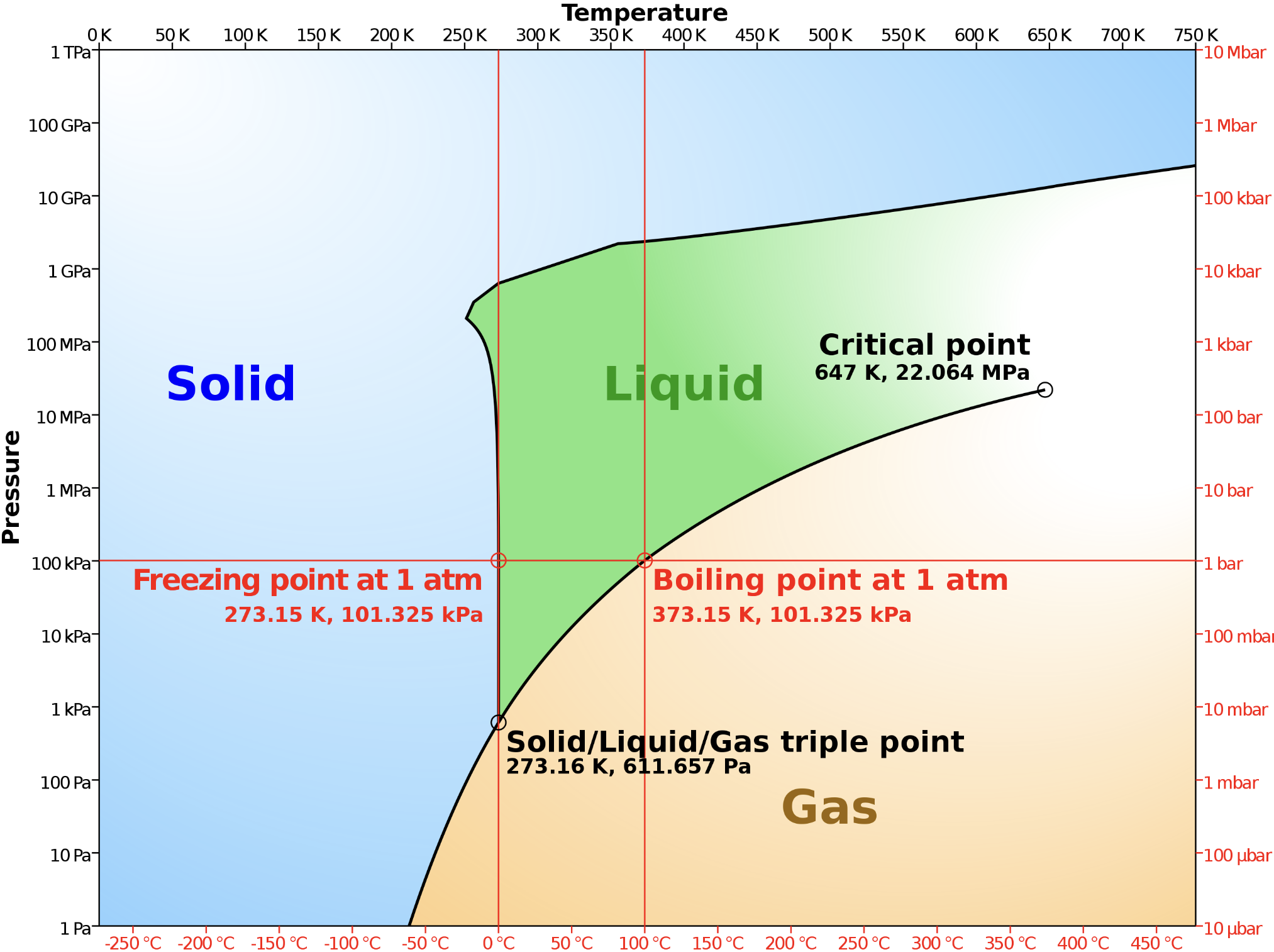
Figure 1: Phase diagrams of (a) (macro-)states of matter of $H_{2}0$ molecules [13]; and (b) of active matter in [14] where $f_{c}^{*}=f_{c}l_{a}/C_{a}$ is the reduced critical force and $\phi_{a}=\pi nl_{a}2$ is the effective “packing fraction” with $C_{a}=1$, $l_{a}=1.3$, $C_{r}=2$, $l_{r}=1.1$ and $D=0$.

The State of the Art

There are certain collective swarm behaviors that have been well studied including flocking, shepherding, shape formation, and collective transport; however, the agents used to create those behaviors are generally sophisticated and often require sensing/actuating/communicating capabilities that are not pragmatic [15, 16, 17, 18, 19]. For example, although sounding fairly simple, smart particle swarms use potential fields that would require the precise states of neighboring agents or at least be able to measure the relative bearings and distances to the neighbors [20, 21, 22].

When the goal of an engineer is a particular emergent behavior, it becomes tempting and easy to simply endow individual agents with enough capabilities to ensure the global behavior can be achieved. Unfortunately this approach does not help understand how exactly a swarm of agents at a certain capability level can exhibit different emergent behaviors. Going back to the water molecules, both chemistry and fluid mechanics study inanimate objects. Water molecules have no agency, they cannot sense their environment or take actions; but, by controlling their environments we can get them to do all sorts of things.

In order to properly study how low-level interactions manifest into group behaviors, we propose that complicated robots makes studying swarms much harder. If even zero-agency water molecules can exhibit different macro-behaviors (e.g., ice, water, vapor) [12], what can a swarm of very simple robots do together? Can simple robots exhibit different ‘states of matter’ depending on their ‘temperature’ and ‘pressure’?

Related Work on Swarm Chemistry

The idea of swarm chemistry by name is not new; it was first proposed by Sayama in 2009 [23] where they found that mixing agents with different control rules led to fascinating new behaviors. However, these swarm chemistry ideas only consider combining two or more different ‘elements’ or ‘species’ together [23, 24, 25]. While this connection is certainly interesting and true, we believe the connection to chemistry goes much deeper and exploring these ideas for even homogeneous agents is a missed opportunity, specifically in regards to the use of phase diagrams as a key tool to predict the phases of the swarm. Phase diagrams used in this way are also not new. Active matter, or substances of self-propelled particles are studied in  [14] for which a similar kind of phase diagram is constructed to determine the macro-state of the system with varying parameters of ‘reduced critical force’ and ‘effective packing fraction,’ Fig. 1(b). However, these earlier works treat the agents as particles and use dynamic rules such as the Boid’s algorithm [26] or similar attractive/repulsive potentials.

We aim to go even further and form a connection between swarms and the field of fluid mechanics as well. Chemistry allows us to know when the macro-state changes in respect to certain environmental conditions, but fluid mechanics goes deeper and describes the characteristics within the different macro states. Continuing our example of water molecules, even within the liquid macro-state we still have complicated behaviors as the water starts moving. The Reynolds number [27] is a dimensionless number known to be a good indicator of whether flowing water is in a laminar or turbulent flow regime. Fig. 2 shows a Moody diagram that plots curves of constant values of relative roughness and draws an empirical relationship between a property of water in its liquid state (the Darcy friction factor) state and the dimensionless Reynolds number [28]. From this figure it is clear to see how even with varying levels of relative roughness, by just looking at the Reynolds number, we can predict the state of the flow since below a certain value ($\sim$2300) the flow is laminar and above another value ($\sim$4000) it is turbulent, with a varying transition regime in between.

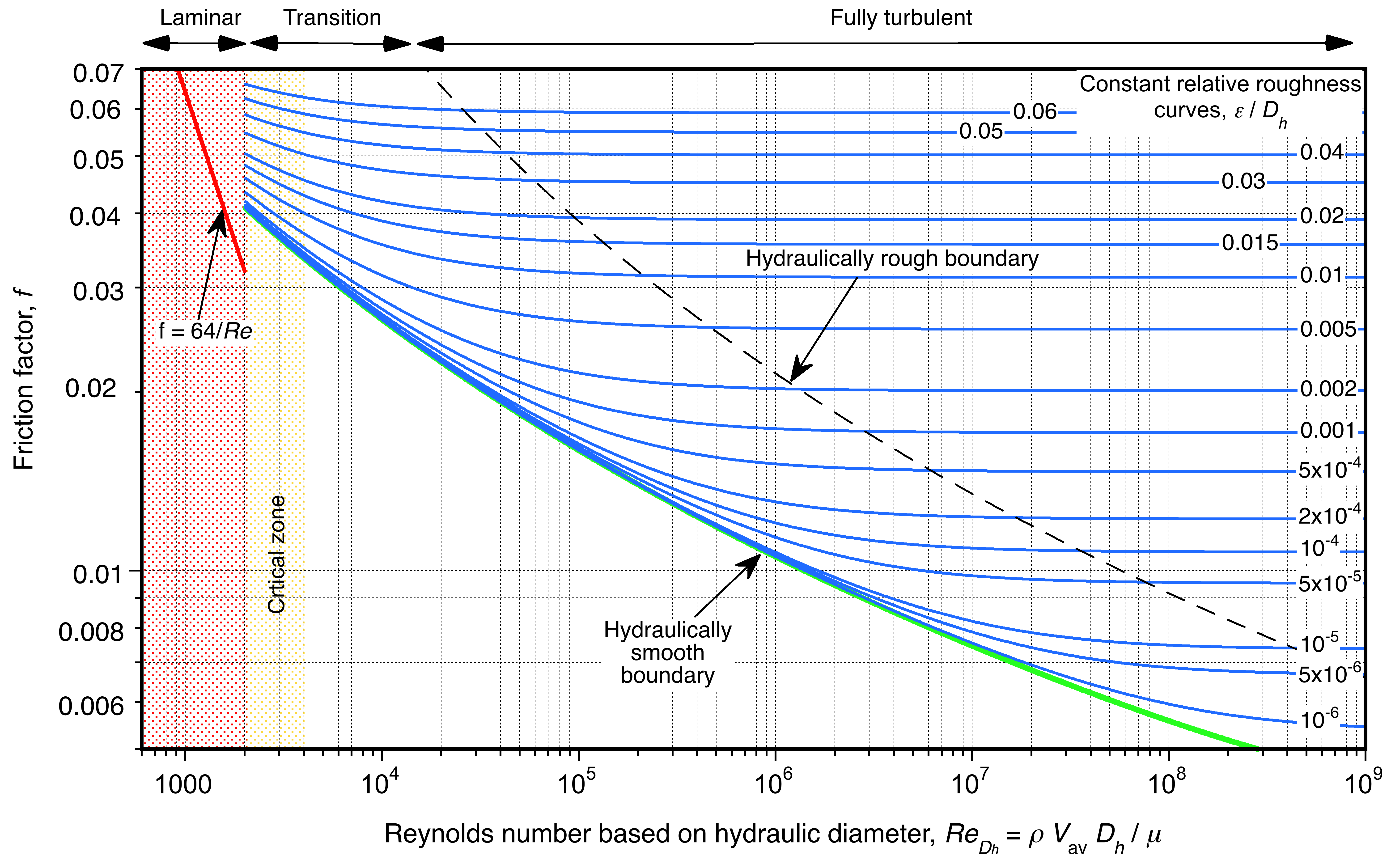
Figure 2: Moody diagram showing the transition from laminar to turbulent flow based on the Reynolds’s number of various relative roughness [28]

Statement of Contributions

This paper presents a novel framework for thinking about robot swarms by drawing connections to chemistry and fluid mechanics. Our contributions are threefold. First, we deepen the connection between swarms and chemistry by showing how phase diagrams can be used to study homogeneous (or single-species) swarms. Rather than focusing on any one particular emergent behavior, we show how small differences in the environmental configurations or inter-agent interaction rules can lead to fundamentally different macro-states. Second, we formalize a brand new connection between swarms and fluid mechanics to seek empirical relationships between the properties of a swarm in a particular macro-state and the agent-level states. Finally, we validate all results in simulation and a few with real robot experiments.

II Problem Formulation

With the goal of formalizing a new framework for swarm analysis, we consider a very simple swarm of $N$ self-propelled Dubins’ vehicles moving in a 2D environment $D\subset{\mathbb{R}}^{2}$. The 2D position and orientation of each robot is given by $p_{i}=(x_{i},y_{i})\in D$ and $\theta_{i}\in[-\pi,\pi)$, respectively, with

$$\left[\begin{array}[]{c}\dot{x}_{i}\\ \dot{y}_{i}\\ \dot{\theta}_{i}\end{array}\right]=\left[\begin{array}[]{c}v\cos\theta_{i}\\ v\sin\theta_{i}\\ u_{i}\end{array}\right].$$ (7)

Our agents only have a binary sensor that is triggered when at least one other agent is within the sensor’s field of view, which is the conical area in front of the robot with range $\gamma>0$ and opening angle $\phi>0$ as shown in Fig. 3 and denoted as $\operatorname{FOV}_{i}$ for agent $i$. We assume that all agents are always moving with a constant velocity $v>0$ and that their turning rate $u_{i}$ is a function of their sensor output. Our goal here is not to design a specific control input to exhibit some desired behavior. Instead, we consider a very simple binary sensing-to-action controller that has already been discovered to exhibit interesting emergent behaviors,

$$u_{i}(z)=\begin{cases}\omega_{\text{max}}&\text{if }\exists j\neq i,s.t.~{}p_{j}\in\operatorname{FOV}_{i},\\ -\omega_{\text{max}}&\text{otherwise,}\end{cases}$$ (8)

where $\omega_{\text{max}}>0$ is the maximum turning rate of the agents. This simple binary controller is capable of producing an emergent behavior where the agents form a rotating circle (or milling) [29, 30, 10, 31], see Fig. 3. However, this mill only appears under certain nontrivial conditions.

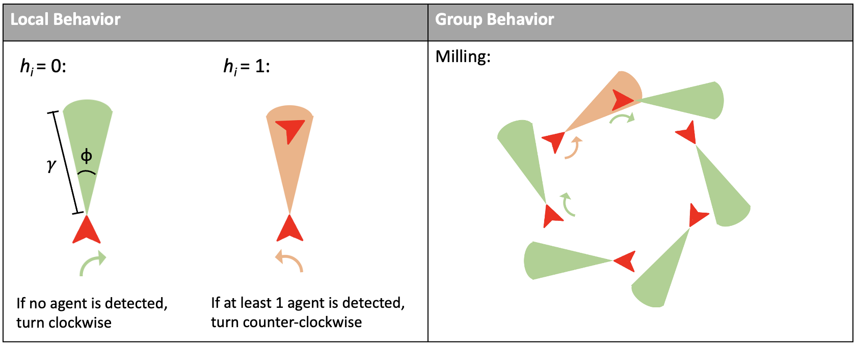
Figure 3: Different local interaction rules leading to different emergent group behaviors (under certain conditions).

Problem II.1 (Characterizing Milling Conditions)

Given the kinematics (7) with direct sensing-to-action controller (8), for what values of $N,v,\omega_{\text{max}},\gamma,$ and $\phi$ does the swarm exhibit the milling behavior shown in Fig. 3?

Problem II.2 (Predicting Properties of Milling)

When the conditions parameterized by $N,v,\omega_{\text{max}},\gamma,$ and $\phi$ give rise to the milling behavior shown in Fig. 3, what is the radius of the emergent circle $R_{m}$?

III Swarm Chemistry

Towards a solution for Problem II.1, we begin by formalizing our new swarm chemistry framework. The aim of this section is to provide tools to enable the full characterization of emergent behaviors from a swarm of agents.

III-A Single Swarm Analysis

Before we can attempt to create our own phase diagrams to try to understand this simple swarm, we must first find a way to evaluate how well the agents are performing the milling behavior of interest at any given time and identify the different possible phases of the swarm. For this, similar to past works [32, 10] we have created our own simple ‘circliness’ metric $c$ defined as

$$c=\frac{R_{out}-R_{in}}{R_{in}}\triangleq\frac{\max_{i\in N}(p_{c}-p_{i})-\min_{i\in N}(p_{c}-p_{i})}{\min_{i\in N}(p_{c}-p_{i})}$$ (9)

where  $p_{c}=(p_{c_{x}},p_{c_{y}})$ is the centroid of the system of agents, different from the center of mass, and its coordinates are

$$p_{c_{x}}=\frac{\max_{i\in N}(p_{i_{x}})-\min_{i\in N}(p_{i_{x}})}{2},$$

$$p_{c_{y}}=\frac{\max_{i\in N}(p_{i_{y}})-\min_{i\in N}(p_{i_{y}})}{2}.$$

With this metric $c=0$ represents a perfect milling circle where all the agents are evenly spaced out in a circle of radius $R_{out}=R_{in}$ as shown in Fig. 4.

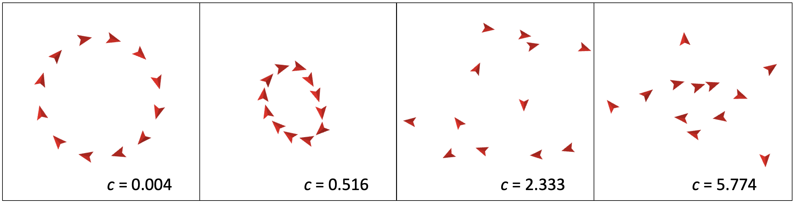
Figure 4: Examples of different values of the circliness metric (9).

We have visually determined that when $c<0.2$ the agents are forming a stable circle and should be classified as being in the milling phase, values of $0.2\leq c<1.5$ create more imperfect ellipsoidal formation, and circliness values higher than that results in unorganized chaos as shown in Fig. 4.

It is important to note that the way we have defined circliness here evaluates any system of less than three agents to be a perfect mill when it doesn’t necessarily create a well shaped circle, therefore we only consider systems of three or more agents before applying this metric.

With these three phases of the simulated swarm of agents, we can make a further connection to chemistry and make an analogy to the phases of matter. The milling phase $M$ has the most structure and can be related to the solid state, the ellipsoidal phase $E$ to a liquid, and the unorganized phase $U$ can be associated with the state of a gas. There is also a seemingly more complicated phase $S$ that will be described in detail in Section III-B.

We can now attempt to create the phase diagrams for this specific simple swarm. The different parameters that can be changed include the number of agents $N$, the forward speed of the agents $v$, turning-rate $\omega_{\text{max}}$, the vision distance $\gamma$, and opening angle of the FOV $\phi$. So these can be set up as the axes similarly to how temperature and pressure are the axes of the water phase diagrams in Fig. 1(a). These parameters clearly appear to have some affect on the resulting behavior. For example, while keeping everything else constant, there appears to be some relationship between $N$ and $\phi$ such that there is only a thin band where milling can occur, Fig. 5. However sweeping through all these parameters results in a multi-dimensional phase space for any configuration of interest in not practical. These figures show how much larger the search space is and motivate novel tools and techniques in generalizing this type of understanding.

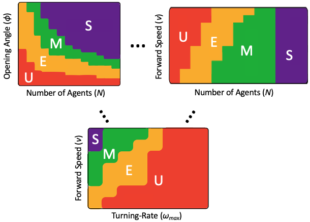
Figure 5: Multiple phase diagrams showing how various conditions can lead to different behaviors. This shows that how these diagrams are only 2D slices of a higher dimensional space.

III-B Multi-Swarm Chemical Analysis

Another issue we ignored about the circliness $c$ is that it assumes all $N$ agents in the system are part of a single swarm or group. Interestingly, as shown in the phase diagrams in Fig. 5, there is an additional $S$ phase. We found that there are certain conditions that lead to scenarios where the system has broken apart into smaller, isolated collections, see Fig. 6(a).

We now need to identify conditions under which a system of $N$ agents should not be viewed as a single group but a collection of two or more sub-swarms. Ultimately we say that when two groups of agents have no influence on each other (including the flow of information), that they should not be considered a single group or swarm.

We formalize this using graph theory to describe the interactions of the swarm to determine when exactly our single swarm system has actually separated into 2 or more groups and should no longer be analyzed collectively by (9) and it should instead be applied separately to each sub-swarm.

A simple method to measure how connected the system is is by looking at the algebraic connectivity of the system using graph theory. We review here only the most pertinent basic information needed but refer readers not familiar with graph theory to [33]. The adjacency matrix of a digraph $\mathcal{G}\triangleq\left(\mathcal{V},\mathcal{E}\right)$ consisting of vertices $\mathcal{V}$ and ordered edges $\mathcal{E}\subseteq{\mathcal{V}}\times{\mathcal{V}}$ is denoted by $A_{\mathcal{G}}=[a_{ij}]$, which is an $N\times N$ matrix defined entry-wise as $a_{ij}=1$ if edge $(v_{j},v_{i})\in\mathcal{E}$, and $a_{ij}=0$ otherwise. The matrix $A_{\mathcal{G}}$ is irreducible if and only if its associated graph $\mathcal{G}$ is strongly connected. The Laplacian is given by $L=D-A$ and the algebraic connectivity is its second smallest eigenvalue $\lambda_{2}(L)$. It is well known that when $\lambda_{2}>0$, the graph ${\mathcal{G}}$ is connected.

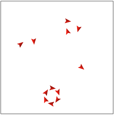
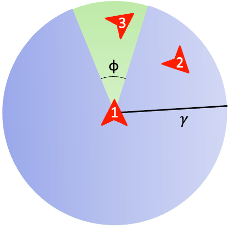
Figure 6: Simulation showing (a) when the system has broken apart into multiple groups, and (b) zooming in on the 3 agents at the top right to view them as a single sub-swarm.

To formalize the notion of a sub-swarm, we begin by constructing the range-limited visibility graph $\mathcal{G}_{\text{vis-disk}}$ from[33] by putting the edge $(v_{j},v_{i})\in E$ if and only if agent $j$ is being seen by agent $i$, i.e., $p_{j}\in\operatorname{FOV}_{i}$. Note that in general this is a dynamic (state-dependent) directed graph and may result in an adjacency matrix that is time-varying and not symmetric. To create an easily verifiable sufficient condition that tells us when the graph is disconnected, we construct a larger but simpler r-disk graph $\mathcal{G}_{\text{disk}}$, where the edge $(v_{j},v_{i})\in E$ if and only if agent $j$ is within $\gamma$ of agent $i$, i.e., $||p_{j}-p_{i}||<\gamma$. Then, if $\mathcal{G}_{\text{disk}}=0$, according to Lemma III.1 below the system is no longer a single swarm.

Lemma III.1

(Sufficient condition for multi-swarm analysis) If $\lambda_{2}(\mathcal{G}_{\text{disk}})=0$, then $\lambda_{2}(\mathcal{G}_{\text{vis-desk}})=0.$

Example III.2 (Connection between ${\mathcal{G}}_{\text{disk}}$ and ${\mathcal{G}}_{\text{vis-disk}}$)

Given the state shown in Fig. 6 (b) with $N=3$, we can construct the adjacency matrices for both $\mathcal{G}_{\text{vis-disk}}$ and $\mathcal{G}_{\text{disk}}$,

$$A_{\mathcal{G_{\text{vis-disk}}}}=\begin{bmatrix}0&0&1\\ 0&0&0\\ 0&0&0\end{bmatrix},~{}~{}~{}~{}A_{\mathcal{G_{\text{disk}}}}=\begin{bmatrix}0&1&1\\ 1&0&1\\ 1&1&0\end{bmatrix}.$$

From this, it is straightforward to see that $\mathcal{G}_{\text{vis-disk}}\subset\mathcal{G}_{\text{disk}}$, and if the larger graph ${\mathcal{G}}_{\text{disk}}$ is not connected, then ${\mathcal{G}}_{\text{vis-disk}}$ must be not connected also. $\bullet$

Rather than just categorizing these scenarios into one broad phase as suggested by the $S$ phase in Fig. 5, we can actually characterize this phase like a chemical mixture of smaller components or sub-swarms. By looking at the connected components of the r-disk graph $\mathcal{G}_{\text{disk}}$, we apply the circliness metric independently to each sub-swarm. For example, we can look at the simulation in Fig. 6(a) made up of 12 agents that has some clearly isolated groups. Rather than characterizing these 12 agents as part of a single chaotic phase, it is much clearer to separate them into their constituent parts. Fig. 6(a) may then be characterized as four sub-swarms, one in the milling phase $M$, one in the ellipsoidal phase $E$, and two in the ‘gas’ phase $U$. Similar to traditional chemical decomposition equations where a single compound breaks down into multiple products, the initially-connected 12-agent system over time naturally separates into smaller subswarms

$$12S\rightarrow 6M+3E+1U+2U.$$

With all the different macro-behaviors characterized, it remains an open question what exactly the ‘temperature’ or ‘pressure’ of the swarm in this context is. It is clear that some empirical relations can be provided based on the phase diagrams but the remaining open question is what functions of these parameters are most representative of the macro states observed?

IV Analyzing Milling

The above methods we call Swarm Chemistry have focused on solving Problem II.1 by determining what macro-state the agents of a swarm are. Although not entirely characterized, we have found conditions in simulation in which the agents self-organize into the milling phase or other macro-states. In this section we want to further analyze a single state of matter (e.g., milling) and find empirical relations between the conditions of the swarm and its macro-state properties. Similar to how the Darcy friction factor of flowing fluid is a function of its Reynold’s number in Fig. 2, can we solve Problem II.2 by finding functions and conditions that predict the radius of the emergent circle $R_{m}$ in the milling phase?

IV-A Existing Work

The work [31] lays the groundwork for obtaining some theoretical limits on the size of a mill that can be formed utilizing the simply binary sensing-to-action method first discovered in [29], and proposes an equation and conditions under which the emergent milling radius can be predicted.

However, the procedure there considers idealized robots and identifies conditions under which agents starting in a milling state should remain there indefinitely. The authors propose an equation that calculates the size of the milling radius formed by agents using field-of-view sensors under certain conditions. Specifically, these conditions are that the individual turning radius of each agent when they don’t detect anything, $r_{0}$ (which is simply the ratio of forward speed to turning rate $\frac{v}{\omega_{\text{max}}}$), must be smaller than or equal to the milling radius: $r_{0}\leq R_{m}$, and that the sensing range $\gamma$ must be sufficiently large in order for the agents to be able to detect one another to form the milling circle,

$$\leavevmode\resizebox{208.13574pt}{}{$\gamma\geq\sqrt{(R_{m}-R_{m}\cos\frac{2\pi}{N}-\rho\cos\frac{\phi}{2})^{2}+(R_{m}\sin\frac{2\pi}{N}+\rho\sin\frac{\phi}{2})^{2}}$},$$ (10)

where $\rho>0$ is the radius (size) of the robot. Finally, the FOV angle $\phi$ should be bounded based on number of robots

$$\phi\leq\frac{2\pi}{N}.$$ (11)

The proposed milling radius from [31] is then

$$R_{m}=\frac{\rho}{cos\frac{\phi}{2}-cos(\frac{2\pi}{N}-\frac{\phi}{2})}.$$ (12)

As far as the authors are aware, this is currently the best answer in the literature to Problem II.2 but we have been unable to independently verify this equation in most cases. Unfortunately, we believe this first solution to be incomplete and that the analysis proposed makes some implicit assumptions along the way that do not generally hold true. The two main issues we identify are that

1. there exist many conditions in which the final periodic orbit is stable but the milling radius $R_{m}$ is oscillating;

2. and the size of the robot $\rho$ has a much more complicated effect on $R_{m}$ than (12) suggests.

We first provide supporting simulation evidence in the form of counterexamples to some statements proposed in [31], then point to some issues we see in the analysis that led to these conclusions.

Following closely the supplemental material provided in [31], the arguments start by analyzing line-of-sight sensors before generalizing this to an integrable FOV with a opening angle $\phi$. With disturbance/noise-free agents and satisfying the conditions (10) and $\eqref{eq:critical}$, it is suggested that when $r_{0}=R_{m}$, the only stable milling configuration is the milling behavior of interest with radius

$$R_{m}=\frac{\rho}{1-\cos\left(\frac{2\pi}{N}\right)},$$

after converging to a set of states with the invariant property that no robot ever sees another robot again. However, we show in Fig. 7 that by simply modifying the starting heading angles we are able to maintain this invariant property while having a milling circle whose radius oscillates around the proposed radius but never settles. Furthermore, depending on the initial conditions of the system it is possible to converge to this periodic limit cycle in which the milling radius never settles. Fig. 7 shows that in this configuration, any particular snapshot of the agents will indeed show a circle but the radius of which may be changing over time. More specifically, the stable mill is only guaranteed for $\phi=\frac{2\pi}{N}$ but may not be true for $\phi<\frac{2\pi}{N}$.

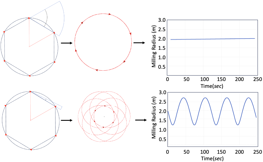
Figure 7: Different behaviors as a result of simply changing $\phi$. The top figure shows the specific starting condition where all six agents are positioned at the vertices of a hexagon with critical $\phi=\frac{\pi}{3}$ that results in a stable milling circle over time. The bottom figure has nearly the same initial configuration except their $\phi=\frac{2\pi}{45}$ which has a drastically different resulting behavior where the measured $R_{m}$ is oscillating.

The second issue is with the size of the agents affecting $R_{m}$ linearly. Intuitively, it is not hard to imagine that as $\rho\rightarrow 0$, it is still possible that small agents make a very large milling circle as we show in Fig. 8; here $\rho$ can arbitrarily be shrunk but $R_{m}$ will not change.

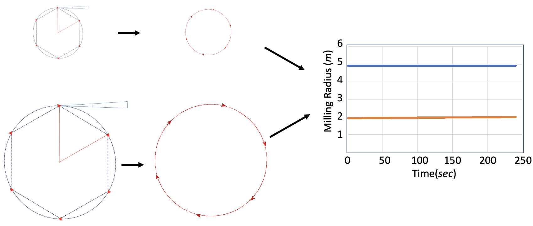
Figure 8: Two separate cases where N = 6, $\phi=\frac{2\pi}{45}$, and $\gamma=8$, the only differences are the turning radius $r_{0}$ and the size of the initial configurations. In the top case, $r_{0}=R_{1}=1.936$ and in the bottom $r_{0}=R_{2}=4.914$; by orienting the agents to point in the direction tangential to the starting circle, the resulting $R_{m}=r_{0}$ in both cases.

IV-B Swarm Mechanics

While the geometric analysis above and in [31] are a good start, the complications stemming from the radius $R_{m}$ being a truly emergent property makes it impractical to use in identifying bounds of operation. For instance, the lower bound on the sensing distance (10) suggests the milling radius $R_{m}$ is an independent variable; but depending on conditions increasing $\gamma$ to satisfy (10) might simultaneously be changing $R_{m}$ and immediately violating (10). A similar argument holds for requiring $r_{0}\leq R_{m}$.

To formalize Problem II.2 a bit further, we wish to find an unknown function $R_{m}=f(N,v,\omega_{\text{max}},\gamma,\phi)\in\mathbb{R}_{\geq 0}\cup\emptyset$ that should return the radius of a mill when the macro-state of the swarm is a mill $M$, and return $\emptyset$ if in any other phase.

To this end, we propose following a route similar to the history of fluid mechanics. The Moody diagram Fig. 2 shows empirical relations between the dimensionless Reynold’s number and the friction factor for varying ‘roughness’. While we one day hope to have a closed-form equation, we can see that even without exact equations a better understanding of how $R_{m}$ depends on the different parameters may be possible by similarly analyzing only certain regimes and providing piece-wise equations based on empirical data. Even the Reynold’s number is not always able to predict correctly if a flow is actually laminar or turbulent, but clearly has been good enough to allow us to control not only which macro-state water is in, but also the properties of water in the different phases. The hope is that this can allow engineers to start actually using collective behaviors of swarms even without a full understanding of how the collective properties emerge. Looking to Fluid Dynamics, the Buckingham Pi Theorem [34] may be useful in reducing the dimension of this problem by lumping parameters together. Here we start with a few empirical relations we have found and hope it motivates others to follow a similar path to deploy emergent behaviors in different starting pockets of predictability, and working to expand from the known areas to the unknown areas of the phase diagrams in Fig 5.

Thus, let us start at one of the simpler cases where $\alpha$ is precisely at the critical value, which is where the equation (12) proposed in [31] seems to have the best chance at some refinement. At this critical angle we have confirmed that for infinite sensing range $\gamma=\infty$, the circle grows indefinitely as (12) suggests. When $\gamma>0$ is fixed, we have confirmed that the milling configuration is generally convergent, but $R_{m}$ varies linearly with the sensing distance $\gamma$ for each $N$.

On the manifold at the critical value $\{\phi=\frac{2\pi}{N}\}$ where this stable circle forms, attempting to calculate the milling radius using (12) results in an undefined answer due to a division by zero error, and values very close to the critical angle results in huge $R_{m}$. In these cases the limiting factor seems to become dependent on the sensing distance $\gamma$, as shown in Fig 9 to help elucidate what happens in [31] when there is a finite sensing range. We find that we are able to almost perfectly combine these relations into a single bilinear equation for systems with critical $\phi=\frac{2\pi}{N}$,

$$R_{m}=(0.1583N+0.043)\gamma+c,$$ (13)

where $c$ is a small constant that varies by less than 5% in this range. The turning radius of the agents affects the final radius of the milling circle only if it is greater than $R_{m}$ as discovered in [31].

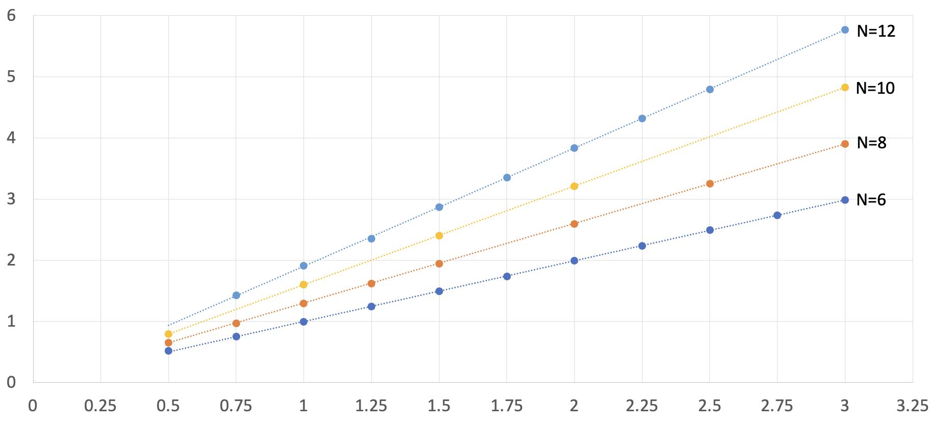
Figure 9: Radius of formed milling behavior changing linearly as sensing range $\gamma$ changes for various $N$ with $\phi=\frac{2\pi}{N}$ and $r_{0}<=R$.

V Robot Validation

Our ultimate goal with the novel framework is to use both simulations and new Swarm Mechanics ideas to deploy real robot swarms with predictable emergent properties. Our companion work on establishing a low-fidelity simulator using our proposed real2sim2real process for swarms [35] allows us to verify behaviors found in simulation on real robots called Flockbots [36].

Naturally it is easier to tune various parameters in simulation than with real hardware. For instance it is not easy to simply tune the FOV angle $\alpha$ of the IR sensors built into the Flockbots and are limited to only being able to use up to $N=11$ of the robots. Fig. 10 shows our simulated phase diagram with a sequence of real robot experiments shown at $\phi=12^{\circ}$ and $N=4,5,6,7,8,9,10,11$ agents. This phase diagram and Swarm Mechanics analysis above allows us to make a hypothesis that we will need $N=13$ robots under the current configuration before we see well-shaped milling circles, and the size of the circle will keep increasing as we add robots until $N=31$ robots when swarm chemistry tells us the circle will be too large to sustain and break out into smaller components. Swarm mechanics helps show us how we expect the radius of the mill to keep growing in Fig. 11 which is our next immedate step.

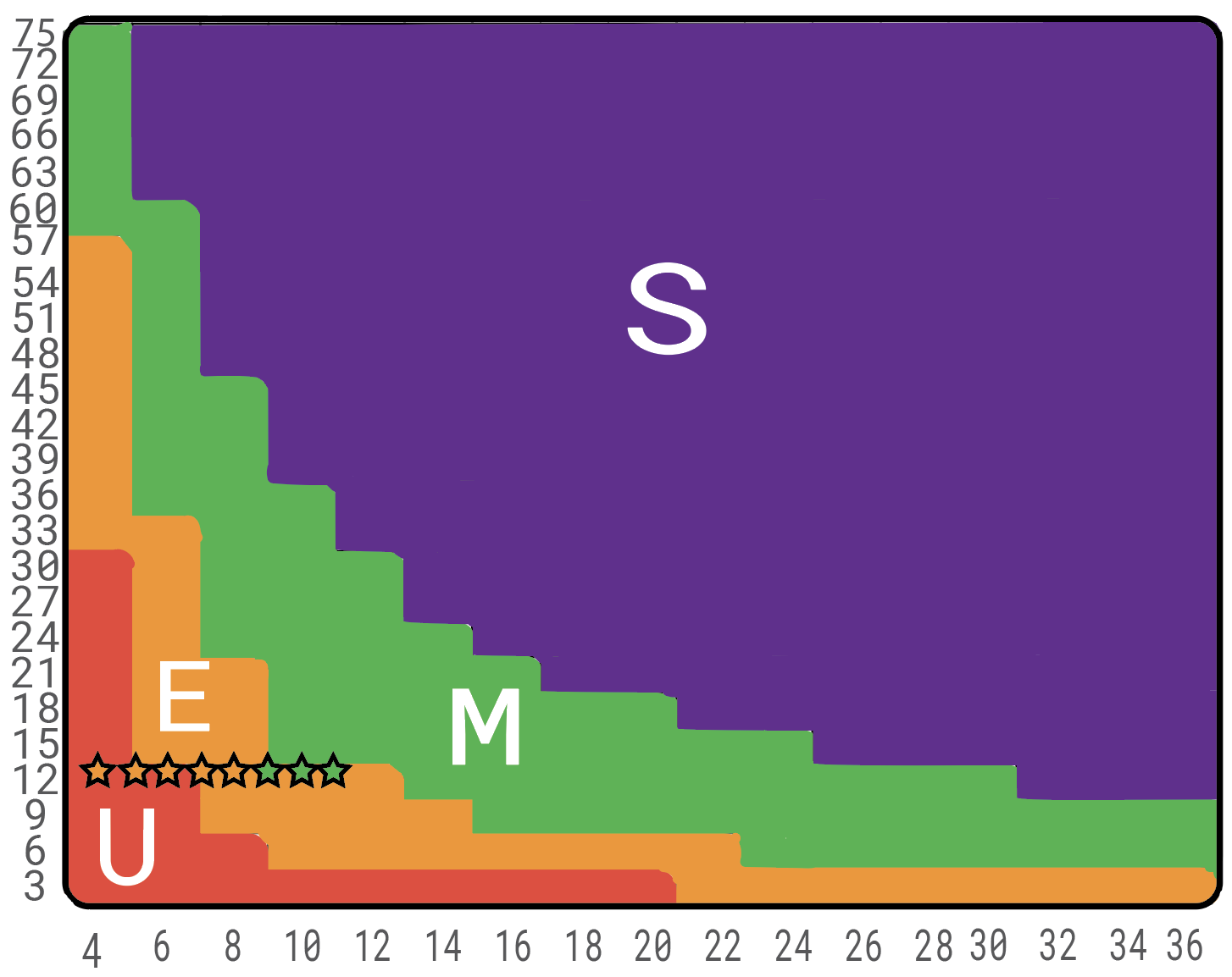
Figure 10: A 2D phase diagram constructed in simulation overlaid with markings showing the impact of $N$ and $\phi$ (in degrees) on the behavior of simulated agents and real Flockbots.

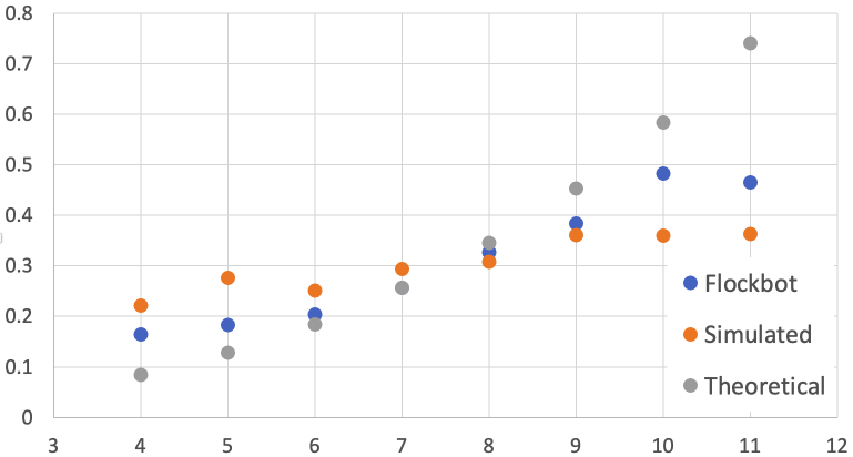
Figure 11: Radius of milling circle formed with various number of agents in our simulator, the proposed equation from [31], and real robot experiments conducted on the Flockbots system

VI Conclusions

This paper proposes a novel approach for analyzing and modeling swarms by turning to chemistry and fluid mechanics for inspiration. The primary contributions in this work are the novel framework and the formulation of new open questions that we believe deserve investigation from the swarms community at large. Our preliminary solutions are naturally incomplete and the goal instead is to draw more attention to these problems and new way of thinking about swarms. Future work will be devoted to seeking a dimensionless number involving only independent parameters that can determine when a milling behavior emerges or not. Our results are validated through both simulations and real experiments on ground robots.

It should be noted that while we applied our novel framework to a simple swarm achieving a specific (already known) behavior, the methods and problems posed can easily be generalized to other swarming phenomena as long as a swarm-level metric is defined.

References

- [1] G. Zhang, G. Fricke, and D. Garg, “Spill detection and perimeter surveillance via distributed swarming agents,” IEEE/asme Transactions on Mechatronics, vol. 18, no. 1, pp. 121–129, 2011.
- [2] H. Kuntze, C. Frey, I.Tchouchenkov, B. Staehle, E. Rome, K. Pfeiffer, A. Wenzel, and J. Wöllenstein, “Seneka-sensor network with mobile robots for disaster management,” in 2012 IEEE Conference on Technologies for Homeland Security (HST), pp. 406–410, IEEE, 2012.
- [3] M. Saska, J. Chudoba, L. Přeučil, J. Thomas, G. Loianno, A. Třešňák, V. Vonásek, and V. Kumar, “Autonomous deployment of swarms of micro-aerial vehicles in cooperative surveillance,” in 2014 International Conference on Unmanned Aircraft Systems (ICUAS), pp. 584–595, IEEE, 2014.
- [4] R. Arnold, J. Jablonski, B. Abruzzo, and E. Mezzacappa, “Heterogeneous uav multi-role swarming behaviors for search and rescue,” in 2020 IEEE Conference on Cognitive and Computational Aspects of Situation Management (CogSIMA), pp. 122–128, IEEE, 2020.
- [5] J. Fromm, “Types and forms of emergence,” arXiv preprint nlin/0506028, 2005.
- [6] J. Fromm, “Ten questions about emergence,” arXiv preprint nlin/0509049, 2005.
- [7] O. Holland, “Taxonomy for the modeling and simulation of emergent behavior systems,” in Proceedings of the 2007 spring simulation multiconference-Volume 2, pp. 28–35, 2007.
- [8] A. Özdemir, M. Gauci, A. Kolling, M. Hall, and R. Groß, “Spatial coverage without computation,” in 2019 International Conference on Robotics and Automation (ICRA), pp. 9674–9680, IEEE, 2019.
- [9] M. Gauci, J. Chen, W. Li, T. Dodd, and R. Groß, “Self-organized aggregation without computation,” The International Journal of Robotics Research, vol. 33, no. 8, pp. 1145–1161, 2014.
- [10] D. St-Onge, C. Pinciroli, and G. Beltrame, “Circle formation with computation-free robots shows emergent behavioral structure,” in IEEE/RSJ International Conference on Intelligent Robots and Systems (IROS), pp. 5344–5349, IEEE, 2018.
- [11] M. Gauci, J. Chen, W. Li, T. Dodd, and R. Groß, “Clustering objects with robots that do not compute,” in Proceedings of the 2014 international conference on Autonomous agents and multi-agent systems, pp. 421–428, 2014.
- [12] B. Predel, M. Hoch, and M. J. Pool, Phase diagrams and heterogeneous equilibria: a practical introduction. Springer Science & Business Media, 2013.
- [13] Wikipedia, “Phase diagram,” https://en.wikipedia.org/wiki/Phase_diagram, 2002.
- [14] N. V. Brilliantov1, H. Abutuqayqah, I. Y. Tyukin, and S. A. Matveev, “Swirlonic state of active matter,” Nature Research Scientific Reports, vol. 10, no. 16783, 2020.
- [15] A. Alfeo, M. Cimino, N. D. Francesco, M. Lega, and G. Vaglini, “Design and simulation of the emergent behavior of small drones swarming for distributed target localization,” Journal of computational science, vol. 29, pp. 19–33, 2018.
- [16] Y. Chuang, Y. R. Huang, M. R. D’Orsogna, and A. L. Bertozzi, “Multi-vehicle flocking: scalability of cooperative control algorithms using pairwise potentials,” in Proceedings 2007 IEEE international conference on robotics and automation, pp. 2292–2299, IEEE, 2007.
- [17] A. Özdemir, M. Gauci, and R. Groß, “Shepherding with robots that do not compute,” in Artificial Life Conference Proceedings, pp. 332–339, MIT Press One Rogers Street, Cambridge, MA 02142-1209, USA journals-info …, 2017.
- [18] Y. Meng, H. Guo, and Y. Jin, “A morphogenetic approach to flexible and robust shape formation for swarm robotic systems,” Robotics and Autonomous Systems, vol. 61, no. 1, pp. 25–38, 2013.
- [19] M. Rubenstein, A. Cabrera, J. Werfel, G. Habibi, J. McLurkin, and R. Nagpal, “Collective transport of complex objects by simple robots: theory and experiments,” in Proceedings of the 2013 international conference on Autonomous agents and multi-agent systems, pp. 47–54, 2013.
- [20] V. Varadharajan, S. Dyanatkar, and G. Beltrame, “Hierarchical control of smart particle swarms,” arXiv preprint arXiv:2204.07195, 2022.
- [21] M. R. D’Orsogna, Y. Chuang, A. L. Bertozzi, and L. S. Chayes, “Self-propelled particles with soft-core interactions: patterns, stability, and collapse,” Physical review letters, vol. 96, no. 10, p. 104302, 2006.
- [22] M. Mabrouk and C. McInnes, “Swarm robot social potential fields with internal agent dynamics,” in 12th International Conference on Aerospace Sciences and Aviation Technology, ASAT-12, 2007.
- [23] H. Sayama, “Swarm chemistry,” Artificial life, vol. 15, no. 1, pp. 105–114, 2009.
- [24] H. Sayama, “Seeking open-ended evolution in swarm chemistry,” in 2011 IEEE Symposium on Artificial Life (ALIFE), pp. 186–193, IEEE, 2011.
- [25] H. Sayama, “Morphologies of self-organizing swarms in 3d swarm chemistry,” in Proceedings of the 14th annual conference on Genetic and evolutionary computation, pp. 577–584, 2012.
- [26] C. Reynolds, “Flocks, herds and schools: A distributed behavioral model,” in Proceedings of the 14th annual conference on Computer graphics and interactive techniques, pp. 25–34, 1987.
- [27] J. Kim, P. Moin, and R. Moser, “Turbulence statistics in fully developed channel flow at low reynolds number,” Journal of fluid mechanics, vol. 177, pp. 133–166, 1987.
- [28] J. G. Leishman, “Introduction to aerospace flight vehicles,” 2022.
- [29] M. Gauci, J. Chen, T. J. Dodd, and R. Groß, “Evolving aggregation behaviors in multi-robot systems with binary sensors,” in Distributed Autonomous Robotic Systems: The 11th International Symposium, pp. 355–367, Springer, 2014.
- [30] D. S. Brown, R. Turner, O. Hennigh, and S. Loscalzo, “Discovery and exploration of novel swarm behaviors given limited robot capabilities,” in Distributed Autonomous Robotic Systems, Springer International Publishing AG, 2018.
- [31] F. Berlinger, M. Gauci, and R. Nagpal, “Implicit coordination for 3d underwater collective behaviors in a fish-inspired robot swarm,” Science Robotics, vol. 6, no. 50, 2021.
- [32] C. Taylor, C. Luzzi, and C. Nowzari, “On the effects of collision avoidance on emergent swarm behavior,” in 2020 American Control Conference (ACC), pp. 931–936, IEEE, 2020.
- [33] F. Bullo, J. Cortés, and S. Martinez, Distributed control of robotic networks: a mathematical approach to motion coordination algorithms, vol. 27. Princeton University Press, 2009.
- [34] J. Evans, “Dimensional analysis and the buckingham pi theorem,” American Journal of Physics, vol. 40, no. 12, pp. 1815–1822, 1972.
- [35] R. Vega, K. Zhu, S. Luke, M. Parsa, and C. Nowzari, “Simulate less, expect more: Bringing robot swarms to life via low-fidelity simulations,” arXiv preprint arXiv:2301.09018, 2023.
- [36] S. Luke, K. Andrea, M. Bowen, D. Fleming, K. Sullivan, B. Hrolenok, C. Vo, A. Bovill, R. Steck, B. Davidson, et al., “The flockbots,” Open specification. Available at http://cs. gmu. edu/ eclab/projects/robots/flockbots, 2014.