No need for an oracle: the nonparametric maximum likelihood decision in the compound decision problem is minimax

Abstract

We discuss the asymptotics of the nonparametric maximum likelihood estimator (NPMLE) in the normal mixture model. We then prove the convergence rate of the NPMLE decision in the empirical Bayes problem with normal observations. We point to (and use) the connection between the NPMLE decision and Stein unbiased risk estimator (SURE). Next, we prove that the same solution is optimal in the compound decision problem where the unobserved parameters are not assumed to be random.

Similar results are usually claimed using an oracle-based argument. However, we contend that the standard oracle argument is not valid. It was only partially proved that it can be fixed, and the existing proofs of these partial results are tedious. Our approach, on the other hand, is straightforward and short.

t1Supported in part by NSF Grant DMS-2113364.

1 Introduction

Suppose, for some unobserved $\vartheta_{1},\dots,\vartheta_{n}$, the observations $Y_{1},\dots,Y_{n}$ are independent given $\vartheta_{1},\dots,\vartheta_{n}$ and $Y_{i}\mid\vartheta_{[n]}\thicksim N(\vartheta_{i},\sigma^{2})$. The goal is to estimate $\vartheta_{[n]}$ under the $L_{2}$ norm,

$$\begin{split}\allowdisplaybreaks{\mathcal{L}}(\vartheta_{[n]},\hat{\vartheta}_{[n]})=\frac{1}{n}\sum_{i=1}^{n}(\hat{\vartheta}_{i}-\vartheta_{i})^{2},\end{split}$$ (1)

where $[n]\triangleq 1,\dots,n$ and for a general sequence, $a_{[n]}$ is a short notation for $a_{1},\dots,a_{n}$.

A few models were considered in the literature to model $\vartheta_{[n]}$. In the classical empirical Bayes (EB) problem, cf. Robbins (1956); Zhang (2003); Efron (2019), $\vartheta_{1},\dots,\vartheta_{n}$ are i.i.d.  $G$ for some unknown $G$. More generally, they may be a time sequence following some state-space model or a hidden Markov model. The statistician’s aim is to minimize $R(G,\hat{\vartheta}_{[n]})\triangleq{\rm E}\mathop{\!}\nolimits{\mathcal{L}}(\vartheta_{[n]},\hat{\vartheta}_{[n]})$ without the knowledge of $G$. Note that the expectation is taken assuming that $\vartheta_{[n]}$ are themselves random. In the compound decision (CD) problems, $\vartheta_{[n]}$ are just fixed unknown parameters. The target now is to minimize the same risk function, but the expectation is taken only over $\hat{\vartheta}_{[n]}$ since $\vartheta_{[n]}$ are fixed. In this paper, we restrict our attention only to the EB/CD problem, i.e., $\vartheta_{1},\dots.\vartheta_{n}$ are either i.i.d.  sample or unknown but fixed. To simplify the discussion, we assume that $|\vartheta_{i}|<c$.

Efron (2019) titled his authoritative Statistical Science review by “Bayes, Oracle Bayes and Empirical Bayes.” Oracle Bayes is what we refer to as the CD problem. Efron’s title brings forward an oracle that essentially makes the CD setup as if it were an EB with respect to the (unknown to the statistician) empirical distribution of the $\vartheta$s. Our main contribution is to argue that this oracle is misleading and unnecessary. We claim that the existence of an asymptotic minimax solution can be proved by the standard method of considering the statistical problem as a zero sum game (with asymmetric information) between the statistician and Nature.

These are two complementary methods to prove that a result is minimax. In both methods, we compare the problem at hand to another problem whose solution is known and serves as a bound of what is achievable. With the oracle, we compare the statistician to a more knowledgeable statistician, which faces an easier problem. In the game theoretic approach, we make Nature more atrocious; thus, the statistician faces a more difficult problem.

We advocate for the nonparametric maximum likelihood estimator (NPMLE) as a good strategy for dealing with both models. It is based on the assumption that the observations come from a mixture of normal distributions as if $\vartheta_{[n]}$ are i.i.d.  (as they are in the EB model but not in the CD one). This approach is based on the connection between the NPMLE and Stein’s unbiased risk estimator (SURE), as presented below. We then bring a new proof that the same solution is indeed valid in the CD context, where seemingly the NPMLE doesn’t fit the model.

Thus the contribution of this communication is threefold: (1) We prove concentration inequality for the NPMLE procedure in the EB and CD problems, (2) We relate the SURE to the NPMLE, and (3) we prove that the NPMLE is minimax in both problems.

2 Maximum likelihood estimator for the empirical Bayes problem

Consider the EB problem described in the introduction. If $G$ were known the optimal decision was the Bayes estimator $\hat{\vartheta}_{i}=\delta_{G}(Y_{i})$, where $\delta_{G}(y)\triangleq{\rm E}\mathop{\!}\nolimits(\vartheta\mid Y=y)$ under the assumption that $\vartheta\thicksim G$ and $Y\mid\vartheta\thicksim\Phi\bigl{(}(\cdot-\vartheta)/\sigma\bigr{)}$, where $\Phi$ is the standard normal cdf. It is well known that $\delta_{G}$ is given by the Tweedie formula, Robbins (1956); Efron (2011, 2019):

$$\begin{split}\allowdisplaybreaks\delta_{G}(y)&=y+\sigma^{2}\frac{f^{\prime}_{G}(y)}{f_{G}(y)},\end{split}$$ (2)

where

$$f_{G}(y) =\frac{1}{\sigma}\int\varphi\bigl{(}\frac{y-\vartheta}{\sigma}\bigr{)}dG(\vartheta)$$

is the marginal density of $Y$. Here $\varphi$ is the standard normal density.

In the EB context, where $G$ is not known, Brown and Greenshtein (2009) proved that we can replace $f_{G}$ by a kernel density estimate of the marginal distribution of $Y$; Greenshtein and Ritov (2022) advocated estimating $f_{G}$ by $f_{\hat{G}}$, where $\hat{G}$ is the nonparametric maximum likelihood (NPMLE) of $G$. In the following, in particular Theorem 2.1, I’ll make their case precise. We start with:

Proposition1 1.

Let $\ell(G;y)=\log f_{G}(y)+y^{2}/2\sigma^{2}$. Then $\delta_{G}(y)-y=\sigma^{2}\ell^{\prime}(G;y)$. The functions $\ell(G;y)$ and $\delta_{G}(y)-y$ have bounded derivatives (with respect to $y$) of any order.

Proof.

Clearly

$$\ell(G;y) =\log\int e^{(y-y_{0})\vartheta/\sigma^{2}}e^{y_{0}\vartheta/\sigma^{2}-\vartheta^{2}/2\sigma^{2}}dG(\vartheta).$$

I.e., it is the log of the moment generating function of $d\tilde{G}_{y_{0}}$ evaluated at $y-y_{0}$, where

$$d\tilde{G}_{y_{0}}\triangleq A\exp({y_{0}\vartheta/\sigma^{2}-\vartheta^{2}/2\sigma^{2}})dG(\vartheta)$$

for some normalizing constant $A=A(G,y_{0})$. It follows that the $k$th derivative of $\ell(G;y)$ with respect to $y$ at $y_{0}$ is the $k$ cumulants of $d\tilde{G}_{y_{0}}$—a distribution with compact support. The $k$th cumulant of any distributions on $(-c,c)$ is bounded by $(2ck)^{k}$ (see Dubkov and Malakhov (1976)).

Since

$$\frac{\partial}{\partial y}\ell(G;y) =\frac{f_{G}^{\prime}(y)}{f_{G}(y)}=\delta_{G}(y)-y,$$

the assertions about $\delta_{G}$ follow. $\square$

In particular:

$$|\delta_{G}(y)| =|{\rm E}\mathop{\!}\nolimits(\vartheta\mid y)|\leq|c|;$$

$$\delta_{G}^{\prime}(y) =\mathop{\rm Var}\nolimits(\vartheta\mid y)\in[0,c^{2}].$$

Note that $\delta_{G}$ is strictly monotone (unless $G$ is a single point mass and $\delta_{G}$ is constant), which follows since the model has the monotone likelihood property.

If $Y\mid\vartheta$ is a mixture of an exponential family with mixing distribution whose support is everywhere dense, then any mean 0 function of $Y$ is in the tangent space. It follows (cf. Bickel et al. (1993); Greenshtein and Ritov (2022)) that

$$\begin{split}\allowdisplaybreaks\int h(y)d{\mathbb{F}}_{n}(y)&=\int h(y)dF_{\hat{G}}(y)+o_{p}(n^{-1/2}),\end{split}$$ (3)

Since $\int h(y)dF_{\hat{G}}(y)=0$ for any $h$ in the tangent set of $\{F_{G}\}$ at $\hat{G}$.

The Stein unbiased risk estimator (SURE) follows the following expansion. Suppose $Y\thicksim N(\vartheta,\sigma^{2})$, then

$${\rm E}\mathop{\!}\nolimits\bigl{(} \delta(Y)-\vartheta)^{2}$$

$$={\rm E}\mathop{\!}\nolimits\bigl{(}\delta(Y)-Y\bigr{)}^{2}+2{\rm E}\mathop{\!}\nolimits\Bigl{(}\bigl{(}\delta(Y)-Y\bigr{)}(Y-\vartheta)\Bigr{)}$$

$$\hskip 30.00005pt+{\rm E}\mathop{\!}\nolimits(Y-\vartheta)^{2}$$

$$={\rm E}\mathop{\!}\nolimits\bigl{(}\delta(Y)-Y\bigr{)}^{2}+2\sigma^{2}{\rm E}\mathop{\!}\nolimits\bigl{(}\delta^{\prime}(Y)-1\bigr{)}+\sigma^{2},$$

where the second term on the RHS follows an integration by part:

$$\int(\delta(y)-y)(y-\vartheta)\frac{1}{\sigma}\varphi\bigl{(}\frac{y-\vartheta}{\sigma}\bigr{)}dy$$

$$=\sigma^{2}\int(\delta^{\prime}(y)-1)\frac{1}{\sigma}\varphi\bigl{(}\frac{y-\vartheta}{\sigma}\bigr{)}dy.$$

Therefore, $\frac{1}{n}\sum_{i=1}^{n}\Bigl{(}\bigl{(}\delta(Y_{i})-Y_{i}\bigr{)}^{2}+2\sigma^{2}\bigl{(}\delta^{\prime}(Y_{i})-1\bigr{)}\Bigr{)}+\sigma^{2}$ is an unbiased estimator of $R(\vartheta_{[n]},\hat{\vartheta}_{[n]})$, where $\hat{\vartheta}_{i}=\delta(Y_{i})$. The Stein unbiased risk estimator is given by ${\rm SURE}(\delta,{\mathbb{F}}_{n})$ where

$${\rm SURE}(\delta;F)$$

$$=\int(\delta(y)-y)^{2}dF(y)+2\sigma^{2}\int(\delta^{\prime}(y)-1)dF(y)+\sigma^{2}.$$

In particular $R(G,\delta)\equiv{\rm SURE}(\delta,F_{G})/n$.

Specializing the definition to the Bayesian estimator $\delta_{G}$ was obtained:

$${\rm SURE}(\delta_{G};{\mathbb{F}}_{n})$$

$$=\sigma^{4}\int\Bigl{(}2\frac{f_{G}^{\prime\prime}(y)}{f_{G}(y)}-\bigl{(}\frac{f_{G}^{\prime}(y)}{f_{G}(y)}\bigr{)}^{2}\Bigr{)}d{\mathbb{F}}_{n}(y)+\sigma^{2}.$$

Now the functions whose mean are computed in the ${\rm SURE}(\delta_{G};{\mathbb{F}}_{n})$ are all with uniformly bounded derivatives and with $L_{2}$ square integrable envelope, since

$$0 \leq\frac{f_{G}^{\prime\prime}(y)}{f_{G}(y)}\leq c^{2}$$

$$0 \leq\bigl{(}\frac{f_{G}^{\prime}(y)}{f_{G}(y)}\bigr{)}^{2}\leq 2y^{2}+2c^{2}.$$

Thus,

$$\begin{split}\allowdisplaybreaks{\rm SURE}(\delta_{\hat{G}};{\mathbb{F}}_{n})&={\rm SURE}(\delta_{\hat{G}},F_{G_{0}})+\operatorname{O_{p}}\left(\sqrt{\frac{\log n}{n}}\right).\end{split}$$ (4)

By 3:

$$\begin{split}\allowdisplaybreaks{\rm SURE}(\delta_{\hat{G}};{\mathbb{F}}_{n})&={\rm SURE}(\delta_{\hat{G}},F_{\hat{G}})+\operatorname{o_{p}}\left(\sqrt{{n}}\right)\end{split}$$ (5)

But

$$\begin{split}\allowdisplaybreaks{\rm SURE}(\delta_{\hat{G}},F_{\hat{G}})&\leq{\rm SURE}(\delta_{G_{0}},F_{\hat{G}})\\ {\rm SURE}(\delta_{G_{0}},F_{G_{0}})&\leq{\rm SURE}(\delta_{\hat{G}},F_{G_{0}}),\end{split}$$ (6)

since $\delta_{\hat{G}}$ minimizes the risk under $\hat{G}$ and $\delta_{G_{0}}$ under $F_{G_{0}}$. Thus,

$${\rm SURE}(\delta_{G_{0}},F_{G_{0}})$$

$$\leq{\rm SURE}(\delta_{\hat{G}},F_{G_{0}}),$$ by 6

$$={\rm SURE}(\delta_{\hat{G}},{\mathbb{F}}_{n})+\operatorname{O_{p}}\left(\sqrt{\frac{\log n}{n}}\right),$$ by 4

$$={\rm SURE}(\delta_{\hat{G}},F_{\hat{G}})+\operatorname{O_{p}}\left(\sqrt{\frac{\log n}{n}}\right),$$ by 5

$$\leq{\rm SURE}(\delta_{G_{0}},F_{\hat{G}})+\operatorname{O_{p}}\left(\sqrt{\frac{\log n}{n}}\right),$$ by 6

$$={\rm SURE}(\delta_{G_{0}},{\mathbb{F}}_{n})+\operatorname{O_{p}}\left(\sqrt{\frac{\log n}{n}}\right),$$ by 3

$$\leq{\rm SURE}(\delta_{G_{0}},F_{G_{0}})+\operatorname{O_{p}}\left(\sqrt{\frac{\log n}{n}}\right), \text{by CLT}.$$

Comparing the LHS, the RHS, and the second line of the display, we obtain that ${\rm SURE}(\delta_{\hat{G}},F_{G_{0}})$ is between ${\rm SURE}(\delta_{G_{0}},F_{G_{0}})$ and ${\rm SURE}(\delta_{G_{0}},F_{G_{0}})+\operatorname{O_{p}}\left(\sqrt{{\log n}/{n}}\right)$. In another form:

Theorem 2.1.

$$R(G_{0},\delta_{\hat{G}_{0}}) =R(G,\delta_{G})+\operatorname{O_{p}}\left(\sqrt{\frac{\log n}{n}}\right).$$

Theorem 2.1 established the asymptotic optimality of using $\delta_{\hat{G}}$. The statistician can achieve without knowing $G$ almost as he could if $G$ was known.

Remark 2.1.

The SURE is defined only with respect to the marginal distribution of $Y$, although it refers to a loss function for some $\vartheta_{1},\dots,\vartheta_{n}$. It is an unbiased estimator of the risk conditioned on $\vartheta_{[n]}$. It obeys uniform LLN and CLT when the set of decision procedures is a VC, as is the case of all Bayes procedures.

3 The Maximum likelihood estimator and the compound decision problem

The optimality for the EB problem was proved by considering an oracle who can do anything the statistician can and knows everything the statistician knows, but unlike the statistician, also knows $G$. Thus, the oracle should use the Bayes procedure $\tilde{\vartheta}_{i}=\delta_{G}(Y_{i})$, and the argument is that the estimator that the statistician is going to use, $\hat{\vartheta}_{i}=\delta_{\hat{G}}(Y_{i})$ has similar performance as is stated in Theorem 2.1.

When we consider the CD problem, this oracle is not useful since he assumes that $\vartheta_{[n]}$ are i.i.d.  $G$, and they are not. It was suggested in the literature, e.g., Jiang and Zhang (2009); Efron (2019) to consider a similar oracle who knows $\vartheta_{[n]}$ up to permutation, effectively their empirical distribution function ${\mathbb{G}}_{n}$, and use $\delta_{{\mathbb{G}}_{n}}$. Then it is argued that $\delta_{{\mathbb{G}}_{n}}$ is comparable to $\delta_{\hat{G}}$ (or any other estimator based on the Tweedie formula 2).

We find this approach to be problematic. An oracle that knows ${\mathbb{G}}_{n}$ will not use $\delta_{\hat{G}}$. Consider the extreme case of $n=2$, and the oracle knows the values $\vartheta_{1}<\vartheta_{2}$, and observe, wlog, $Y_{1}<Y_{2}$. In that case he would consider the pairing $(\vartheta_{1},Y_{1}),(\vartheta_{2},Y_{2})$ as more likely than the other pairing $(\vartheta_{1},Y_{2}),(\vartheta_{2},Y_{1})$. Certainly, if $Y_{2}-Y_{2}\gg\sigma$. Greenshtein and Ritov (2009, 2019) argue that the minimax decision for this particular oracle is the permutation invariant estimator

$$\delta^{*}_{{\mathbb{G}}_{n}}(Y_{i};Y_{[n]})$$

$$=\frac{\sum_{j=1}^{n}\vartheta_{j}\varphi\bigl{(}\frac{Y_{i}-\vartheta_{j}}{\sigma}\bigr{)}\sum_{\pi\in\Pi_{n}(i,j)}\prod_{k\neq i}\varphi\bigl{(}\frac{Y_{k}-\vartheta_{\pi(k)}}{\sigma}\bigr{)}}{\sum_{j=1}^{n}\varphi\bigl{(}\frac{Y_{i}-\vartheta_{j}}{\sigma}\bigr{)}\sum_{\pi\in\Pi_{n}(i,j)}\prod_{k\neq i}\varphi\bigl{(}\frac{Y_{k}-\vartheta_{\pi(k)}}{\sigma}\bigr{)}},$$

where $\Pi_{n}(i,j)$ is the set of all permutations of $1,\dots,n$ such that $\pi(i)=j$ for every $\pi\in\Pi_{n}(i,j)$. This estimator uses all of $Y_{[n]}$ to estimate $\vartheta_{i}$.

Thus, the oracle should be somehow prevented from using the optimal (for him) procedure. One approach was to enforce the oracle to use a ‘simple’ or ‘separable’ estimator such that $\hat{\vartheta}_{i}$ depends on the observations only through $Y_{i}$. Indeed, an oracle thus restricted should use $\delta_{{\mathbb{G}}_{n}}$. However, we cannot compare him to the statistician: He, the oracle, knows better but is more restricted than the human statistician. The estimator $\delta_{\hat{G}}(Y_{i})$ the statistician is using is not simple and uses all the observations (through $\hat{G}$) for the estimate $\hat{\vartheta}_{i}$.

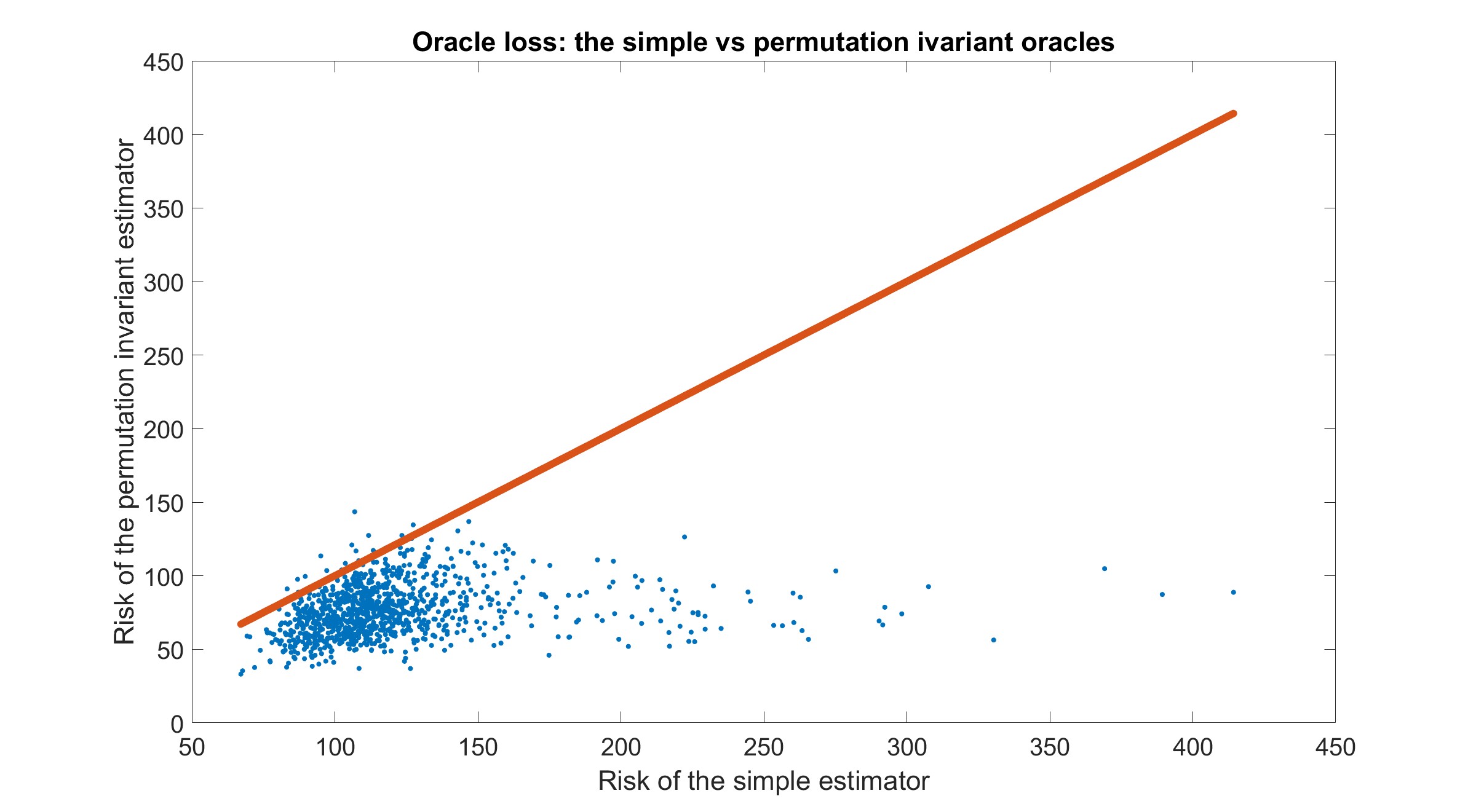
(a)

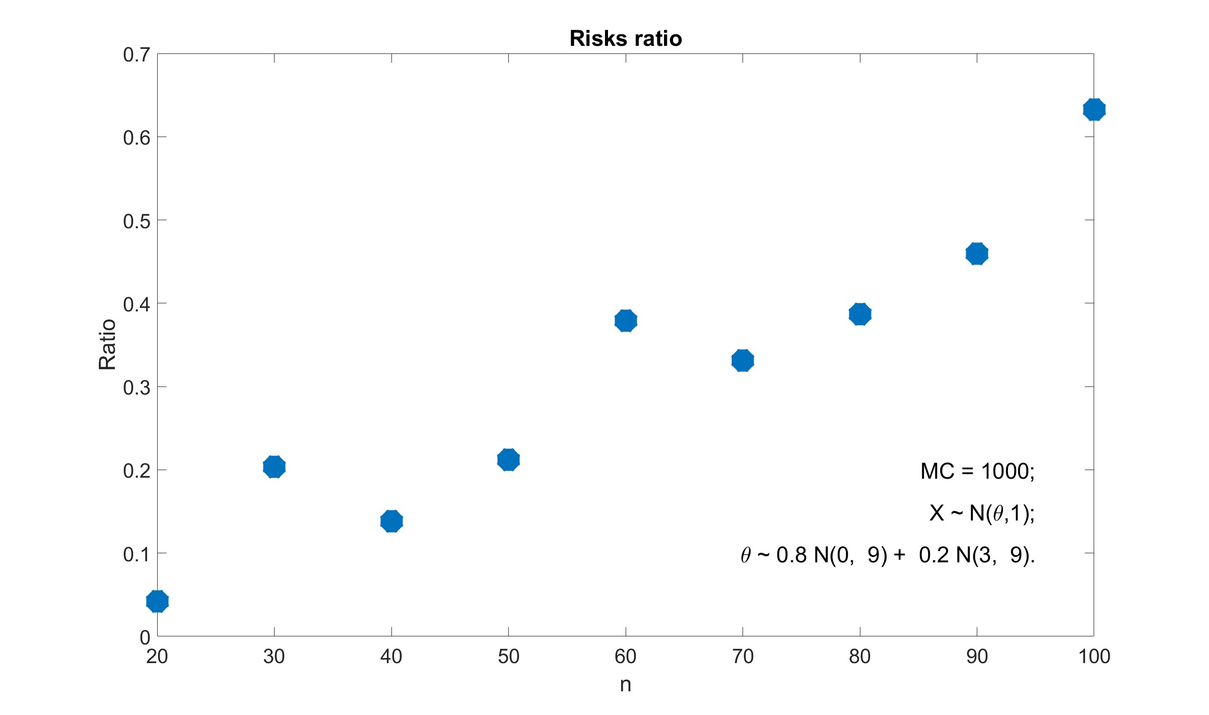
(b)

Figure 1: Comparing the risks of the estimators. The permutation invariant estimator is based on 1000000 random permutations. The $Y\thicksim N(\vartheta,1)$, while $\vartheta$ is with probability 0.8 a $N(0,9)$ rv and with probability 0.2, $N(3,9)$. (a) The loss function of the permutation invariant estimators on 1000 samples vs. the loss of the simple estimators applied to the same samples. The sample size was $n=100$; (b) The efficiency of the permutation invariant estimator relative to that of the simple estimator as a function of sample size $n$. Each point is based on 1000 Monte Carlo trials.

The difference between $\delta_{{\mathbb{G}}_{n}}$ and $\delta^{*}_{{\mathbb{G}}_{n}}$ is considerable even with moderate to large sample. The optimal oracle procedure is uncomputable, but we can approximate it by a biased sample of random permutations, where permutations are weighted independently of $Y_{[n]}$, according to their likelihood under $\vartheta_{[n]}$. In Figure 1, we compare the simple estimator, $\delta_{{\mathbb{G}}_{n}}$, to the biased sample approximation, and the approximate permutation invariant estimator is strictly better up to $n=100$. Similar simulations were presented in Greenshtein and Ritov (2019). It is true that, asymptotically, the two estimators seem to be equivalent. It was proved in Greenshtein and Ritov (2009) that under specific conditions $R({\mathbb{G}}_{n},\delta_{\hat{G}})=R({\mathbb{G}}_{n},\delta^{*})+\operatorname{o_{p}}\left(1\right)$. But the argument is tedious, and the conditions are strong, while it is unclear whether this oracle makes sense.

Example 3.1.

Consider $\vartheta_{i}=\tau_{i}+\xi_{i}$ where $\xi_{i}\thicksim{\mathcal{N}}(0,1)$ and $\tau_{i}/c_{n}$ is uniform of $1,\dots,k_{n}$ for some $c_{n}\to\infty$ and $n/k_{n}\to m$. Thus, the oracle is faced by $k_{n}$ separated clusters, each of size $m$. All the random variables are independent. But, for any $m$, the permutation invariant estimator is strictly better than the simple estimator. We conclude that the argument based on the oracle fails to prove the efficiency of the EB estimator in this CD problem.

4 Asymptotic efficiency of the NPMLE for the CD problem

Our approach is different. There are other approaches to prove the optimality of a procedure. If the oracle method compared the statistician to a better decision maker, the classical approach was to give Nature more freedom and consider a zero-sum game in which the minimizer, the statistician, chooses a procedure and the maximizer, Nature, chooses a parameter with payoff.

We consider a game between the Statistician and Nature. If we let Nature choose any $\vartheta_{[n]}$, He would select the global minimax solution, cf. Bickel (1981), which would not be relevant to our real statistical realm in which there are some arbitrary $\vartheta_{[n]}$ and not the worst possible. We want to adapt to these arbitrary points. To consider adaptive estimator while keeping the minimax notion, we commonly restrict Nature to be in some neighborhood. Thus, we have the local minimax in the sense of Hájek and Le Cam, or more generally, the adaptive estimation in the semiparametric models. We follow these ideas.

The game: For a giving $G$ let ${\mathcal{G}}$ be the set of all random (or not) probability distribution functions, such that if $\{{\mathbb{G}}_{n}\}\in{\mathcal{G}}$ then ${\rm E}\mathop{\!}\nolimits{\mathbb{G}}_{n}=G$ and ${\mathbb{G}}_{n}(t)=\frac{1}{n}\sum_{i=1}^{n}\mbox{\large$1{\sf I}$}(\vartheta\leq\vartheta_{i})$ for some $\vartheta_{1},\dots,\vartheta_{n}$. The statistician observes $Y_{[n]}$ which are independent given $\vartheta_{[n]}$ and $Y_{i}\thicksim{\mathcal{N}}(\vartheta_{i},\sigma^{2})$. He, the statistician, who neither knows $G$ nor ${\mathbb{G}}_{n}$, has to choose $\hat{\vartheta}_{[n]}=\Delta(Y_{[n]})$, $\Delta:{\mathbb{R}}^{n}\to{\mathbb{R}}^{n}$, with payoff given by 1. The value of the game is $R({\mathbb{G}}_{n},\Delta)=E{\mathcal{L}}(\vartheta_{[n]},\hat{\vartheta}_{[n]})$.

Note that ${\mathbb{G}}_{n}$ in the definition of $R(\cdot,\cdot)$ is a random element. Thus the expectation is also over the (possibly) random $\vartheta_{[n]}$.

Theorem 4.1.

Asymptotically, $\delta_{\hat{G}}$ is a minimax strategy, and ${\mathbb{G}}_{n}$, an empirical distribution function of a random sample from $G$, is a maxmin strategy for Nature. The conclusion of Theorem 2.1 is valid for the game.

The proof of the theorem is immediate. If ${\mathbb{G}}_{n}$ is the edf of an i.i.d.  sample from $G$, then ${\rm E}\mathop{\!}\nolimits{\mathbb{G}}_{n}=G$, and since for any given procedure of the statistician, the reward for Nature is linear in ${\mathbb{G}}_{n}$, the value for each ${\mathbb{G}}_{n}\in{\mathcal{G}}$ is the same and is a function only of $G$. On the other hand, if ${\mathbb{G}}_{n}$ is i.i.d.  edf, then we are back in the EB setup, and hence $\delta_{\hat{G}}$ is approximately optimal. Thus $({\mathbb{G}}_{n},\delta_{\hat{G}})$ is an asymptotic saddle point.

We express the result from the point of view of the statistician:

Theorem 4.2.

If $\Delta_{\hat{G}}=\bigl{(}\delta_{\hat{G}}(Y_{1}),\dots,\delta_{\hat{G}}(Y_{n})\bigr{)}$, then for any ${\mathbb{G}}_{n}\in{\mathcal{G}}$:

$$R({\mathbb{G}}_{n},\Delta_{\hat{G}}) \leq\min_{\Delta}\max_{\tilde{}{\mathbb{G}}_{n}\in{\mathcal{G}}}R(\tilde{}{\mathbb{G}}_{n},\Delta)+\operatorname{O_{p}}\left(\sqrt{\frac{\log n}{n}}\right).$$

Note that if Nature “chooses” some fixed $\vartheta_{[n]}$. then we can simply take ${\mathcal{G}}$ to be a point mass at ${\mathbb{G}}_{n}$.

We considered a specific restriction on Nature, namely ${\mathbb{G}}_{n}\in{\mathcal{G}}$. We could replace it with other restrictions. For example, we could consider $\{{\mathbb{G}}_{n}\}\in\tilde{}{\mathcal{G}}$ if ${\mathbb{G}}_{n}\stackrel{{\scriptstyle w}}{{\Rightarrow}}G$, since then $R({\mathbb{G}}_{n},\Delta)\to R(G,\Delta)$ by the definition of weak convergence.

References

- Bickel (1981) {barticle}[author] \bauthor\bsnmBickel, \bfnmPeter J\binitsP. J. (\byear1981). \btitleMinimax estimation of the mean of a normal distribution when the parameter space is restricted. \bjournalThe Annals of Statistics \bvolume9 \bpages1301–1309. \endbibitem
- Bickel et al. (1993) {bbook}[author] \bauthor\bsnmBickel, \bfnmPeter J\binitsP. J., \bauthor\bsnmKlaassen, \bfnmChris AJ\binitsC. A., \bauthor\bsnmBickel, \bfnmPeter J\binitsP. J., \bauthor\bsnmRitov, \bfnmYa’acov\binitsY., \bauthor\bsnmKlaassen, \bfnmJ\binitsJ., \bauthor\bsnmWellner, \bfnmJon A\binitsJ. A. and \bauthor\bsnmRitov, \bfnmYA’Acov\binitsY. (\byear1993). \btitleEfficient and adaptive estimation for semiparametric models \bvolume4. \bpublisherSpringer. \endbibitem
- Brown and Greenshtein (2009) {barticle}[author] \bauthor\bsnmBrown, \bfnmLawrence D.\binitsL. D. and \bauthor\bsnmGreenshtein, \bfnmEitan\binitsE. (\byear2009). \btitleNonparametric Empirical Bayes and Compound Decision Approaches to Estimation of a High-Dimensional Vector of Normal Means. \bjournalThe Annals of Statistics \bvolume37 \bpages1685–1704. \endbibitem
- Dubkov and Malakhov (1976) {barticle}[author] \bauthor\bsnmDubkov, \bfnmAA\binitsA. and \bauthor\bsnmMalakhov, \bfnmAN\binitsA. (\byear1976). \btitleProperties and interdependence of the cumulants of a random variable. \bjournalRadiophysics and Quantum Electronics \bvolume19 \bpages833–839. \endbibitem
- Efron (2011) {barticle}[author] \bauthor\bsnmEfron, \bfnmBradley\binitsB. (\byear2011). \btitleTweedie’s Formula and Selection Bias. \bjournalJournal of the American Statistical Association \bvolume106 \bpages1602-1614. \bnotePMID: 22505788. \bdoi10.1198/jasa.2011.tm11181 \endbibitem
- Efron (2019) {barticle}[author] \bauthor\bsnmEfron, \bfnmBradley\binitsB. (\byear2019). \btitleBayes, Oracle Bayes and Empirical Bayes. \bjournalStatistical Science \bvolume34 \bpagespp. 177–201. \endbibitem
- Greenshtein and Ritov (2009) {barticle}[author] \bauthor\bsnmGreenshtein, \bfnmEitan\binitsE. and \bauthor\bsnmRitov, \bfnmYa’acov\binitsY. (\byear2009). \btitleAsymptotic efficiency of simple decisions for the compound decision problem. \bjournalLecture Notes-Monograph Series \bpages266–275. \endbibitem
- Greenshtein and Ritov (2019) {barticle}[author] \bauthor\bsnmGreenshtein, \bfnmEitan\binitsE. and \bauthor\bsnmRitov, \bfnmYa’acov\binitsY. (\byear2019). \btitleComment: Empirical Bayes, compound decisions and exchangeability. \endbibitem
- Greenshtein and Ritov (2022) {barticle}[author] \bauthor\bsnmGreenshtein, \bfnmEitan\binitsE. and \bauthor\bsnmRitov, \bfnmYa’acov\binitsY. (\byear2022). \btitleGeneralized maximum likelihood estimation of the mean of parameters of mixtures. With applications to sampling and to observational studies. \bjournalElectronic Journal of Statistics \bvolume16 \bpages5934–5954. \endbibitem
- Jiang and Zhang (2009) {barticle}[author] \bauthor\bsnmJiang, \bfnmWenhua\binitsW. and \bauthor\bsnmZhang, \bfnmCun-Hui\binitsC.-H. (\byear2009). \btitleGeneral maximum likelihood empirical Bayes estimation of normal means. \endbibitem
- Robbins (1956) {bmisc}[author] \bauthor\bsnmRobbins, \bfnmH\binitsH. (\byear1956). \btitleAn Empirical Bayes approach to statistics. In proceedings of the third Berkeley symposium of mathematical statistics and probability. \endbibitem
- Zhang (2003) {barticle}[author] \bauthor\bsnmZhang, \bfnmCun-Hui\binitsC.-H. (\byear2003). \btitleCompound Decision Theory and Empirical Bayes Methods. \bjournalThe Annals of Statistics \bvolume31 \bpages379–390. \endbibitem