On Localization of the Fractional Discrete Nonlinear Schrödinger Equation

Abstract

The continuum and discrete fractional nonlinear Schrödinger equations (fDNLS) represent new models in nonlinear wave phenomena with unique properties. In this paper, we focus on various aspects of localization associated to fDNLS featuring modulational instability, asymptotic construction of onsite and offsite solutions, and the role of Peierls-Nabarro barrier. In particular, the localized onsite and offsite solutions are constructed using the map approach. Under the long-range interaction characterized by the Lévy index $\alpha>0$, the phase space of solutions is infinite-dimensional unlike that of the well-studied nearest-neighbor interaction. We show that an orbit corresponding to this spatial dynamics translates to an approximate solution that decays algebraically. We also show as $\alpha\rightarrow\infty$, the discrepancy between local and nonlocal dynamics becomes negligible on a compact time interval, but persists on a global time scale. Moreover it is shown that data of small mass scatter to free solutions under a sufficiently high nonlinearity, which proves the existence of strictly positive excitation threshold for ground state solutions of fDNLS.

Keywords. nonlinear modes, localization, stability, asymptotic approximation, nonlocal dynamics

MSC 2020 34A08, 34A12, 34A34, 37K45, 37K60, 78M35

1 Introduction.

Research in arrays of coupled nonlinear oscillators remains a field of intense research whether it aims at understanding thermalization or the emergence of localized coherent structures, or global synchronization as exemplified by the FPUT or the Kuramoto oscillator model, respectively. Their relevance goes beyond theory as they model systems in a wide range of applications including photonics, plasmonics [1, 2, 3], Bose-Einstein condensates [4, 5, 6, 7], biological/chemical phenomena [8, 9], neuroscience [10] and the power grid [11]. For more comprehensive surveys, see [12, 13, 14, 15]. In all these cases, the emerging models are large systems of coupled ordinary differential equations. Similarly for continuous fields, universal equations such as the nonlinear Schrödinger equation (NLSE) or the sine-Gordon equation have provided a platform to study many features in nonlinear wave phenomena including the existence and interactions of solitons, and the formation of coherent structures and singular blow-up dynamics.

Specific to nonlinear photonics and its applications, two universal models are the NLSE and the discrete nonlinear Schrödinger equation (DNLS) (1.3). In the discrete case, the model describes waveguide or resonator arrays with the nearest-neighbor coupling, whereas the continuum version models, for example, pulses in optical fibers or light filaments propagating in air. In this paper, we present results for nonlocal, nonlinear discrete systems, departing from the nearest-neighbor coupling, whose long-range interaction is described by a nonlocal interaction kernel whose coupling strength decays algebraically. This model is known as the fractional discrete nonlinear Schrödinger equation (fDNLS) given by

$$i\dot{u}_{n}=\epsilon\sum_{m\in\mathbb{Z}\setminus\{n\}}\frac{u_{n}-u_{m}}{|n-m|^{1+\alpha}}-|u_{n}|^{2}u_{n},\ (n,t)\in\mathbb{Z}\times\mathbb{R},\ \epsilon>0,\ \alpha>0,$$ (1.1)

where our interest goes beyond this specific model to study a general long-range interaction given by (2.2). Such nonlocal model was previously studied [16, 17, 18, 19, 20] in various contexts including stability, chaos, and higher-dimensional dynamics.

Unlike the vast amount of experimental results on waveguide arrays modeled by the DNLS, at time there is no concrete photonics-based array for which the fDNLS is an experimentally-verifiable model. We do believe, however, the results could pave the way to future realizations where non-locality presents a new degree of freedom. It should be noted that the continuum version of the fDNLS

$$i\partial_{t}U=(-\Delta)^{\frac{\alpha}{2}}U-|U|^{2}U,\ (x,t)\in\mathbb{R}^{d+1},$$ (1.2)

where $U(x,t)\in\mathbb{C}$ models, for example, the envelope dynamics of an electric field, was proposed as a model for an optical cavity [21] whereby a proper design of lenses allows one to engineer diffraction to behave as $|k|^{\alpha},\ 0<\alpha<2$ in the Fourier representation. The suggested benefit of such a design is to produce laser beam outputs with unique (Airy-like) profiles as opposed to the classical Gaussian-like outputs.

The continuum and discrete dynamics, either viewed as a discretization of a continuum model, or in reverse, the continuum limit of an intrinsically discrete model, exhibit distinct features, one of them being the Peierls-Nabarro Barrier (PNB) in the discrete model [22, 23, 2]. Of central concern in the theory of nonlinear lattices is the propagation of localized waves in discrete media. A motion along the lattice requires the localized wave to switch its structure from onsite to offsite, and vice versa, interacting with the effective energy potential barrier, or the PNB, rising from the inherent discreteness of the lattice. The continuum power-type NLSE, say (1.2) with $\alpha=2$, satisfies the Galilean invariance: if $u(x,t)$ is a solution for $x\in\mathbb{R}^{d}$, then so is $e^{i\frac{v}{2}\cdot(x-\frac{tv}{2})}u(x-vt,t)$ for any $v\in\mathbb{R}^{d}$. In particular, a ground state solution can be boosted to yield a family of solutions whose amplitudes are traveling waves. Moreover the mass-critical NLSE is invariant under the pseudoconformal symmetry, which could be used to show the existence of excitation threshold of mass [24, 25] for certain NLSE with sufficiently high nonlinearity. On the other hand, the lattice structure lacks these symmetries rising from the smooth structure of the Euclidean space, giving rise to, among many others, a non-zero PNB. We confirm the presence of nonlocal PNB in our asymptotic analysis where the energy difference between onsite and offsite solutions is computed explicitly. Our theory is supported by numerical simulations of the dynamics of (1.1) for varying degrees of non-locality where localized solutions with an initial boost are eventually pinned at a lattice site.

On the other hand, the role of non-locality and discreteness on the formation of localized states by modulational instability (MI) is investigated. A periodic train of pulses, under a small perturbation in its spectrum that originates from nonlinearity, localizes as a breather-like excitation driven by MI. The literature on MI is vast, and for our purposes, readers are directed to [26, 27, 28, 29, 30, 31] for survey results with applications in nonlinear optics or fluid dynamics. However a detailed analysis of MI of nonlocal dynamics is still at its infancy. See [32] for MI in relation to the fractional NLSE. Furthermore see [33] that investigates the mixed-fractional NLSE in the context of MI.

While this paper only discusses the discrete model, observe in (1.1) that by considering $\epsilon=c(d,\alpha)h^{-\alpha}$ where $c(d,\alpha)$ is given by (2.5) and $\alpha\in(0,2)$, (1.1) could be understood as a finite difference scheme of the continuum fNLSE (1.2). The well-posedness theory of (1.2) requires a more delicate analysis than its discrete version (see Proposition 3.1) given that blow-up phenomena could occur [34]. See [35, 36] for the rigorous analysis of the well-posedness of fNLSE in Sobolev spaces. The functional-analytic tools of the aforementioned references do not directly apply when the non-locality, represented by the linear dispersion relation, is not uniform in space (which occurs when the spatial dimension is at least two), and thus to account for such non-homogeneity that rises in the mixed-fractional NLSE, the non-smooth analogue of the Littlewood-Paley theory was developed to establish the well-posedness in anisotropic Sobolev spaces [37].

Even with the continuum model being well-posed for data of sufficiently high regularity, it is not trivial to show the continuum limit as $h\rightarrow 0$, if it holds at all. For example, the mass-critical cubic NLSE on $\mathbb{R}^{2}$ contains solutions that blow up in finite time whereas the lattice dynamics is always global. It was shown rigorously in [38] that the weak convergence of nonlocal discrete to continuum dynamics of the Schrödinger evolution holds. A further research done by [39] (see references therein) refined the weak to strong convergence by employing discrete Strichartz estimates uniform in the discreteness parameter. Furthermore note [40] for the first result in the continuum limit of fDNLS to fNLSE in dimension two. In the context of onsite/offsite solutions, it is expected that the PNB would tend to zero in the continuum limit since the Galilean invariance needs to be recovered. This is indeed true, and moreover the quantitative bound that PNB vanishes exponentially fast as $h\rightarrow 0$ was shown in [41, 42] for DNLS and fDNLS, respectively.

This paper is organized as follows. In Section 2, the main model and its properties are introduced. In Section 3, the global dynamics corresponding to $\alpha\gg 1$ is investigated. In the formal limit as $\alpha\rightarrow\infty$, (1.1) converges to the DNLS

$$i\dot{u}_{n}=-\epsilon\delta^{2}u_{n}-|u_{n}|^{2}u_{n},\ (n,t)\in\mathbb{Z}^{d}\times\mathbb{R},\ \epsilon>0,$$ (1.3)

with $d=1$, where $\delta^{2}u_{n}:=\sum\limits_{|j-n|=1}u_{j}-2du_{n}$ and $|\cdot|$ defined with the $l^{1}$ norm on $\mathbb{Z}^{d}$. The nature of this limit, whether it is regular or singular, is subtle as it relates to the Soliton Resolution Conjecture and the long-time dynamics of Hamiltonian systems whose solutions do not dissipate. In Section 4, linear stability analysis on the CW solution of fDNLS is shown with explicit regions of MI. The onset of nonlinear bound states resulting from MI is shown via numerical simulations. In Section 5, the family of onsite and offsite solutions and the corresponding PNB are constructed asymptotically for DNLS and fDNLS, respectively. Although the rigorous aspects of numerical analysis (consistency, convergence, etc) are not our main focus, we provide the numerical discretization of the fractional Laplacian in Appendix A.

2 Background.

In this paper, we consider the generalized nonlocal model, also considered in [38], where the infinitesimal generator is given by

$$\mathscr{L}_{\alpha}f_{n}=\sum_{m\neq n}J_{|n-m|}(f_{n}-f_{m}),\ (f_{n})\in l^{2}(\mathbb{Z}),\ \alpha>0,$$ (2.1)

where $J=(J_{n})_{n=1}^{\infty},\ J_{n}\geq 0$ is the $\alpha$-kernel satisfying the limit property

$$\lim\limits_{n\rightarrow\infty}n^{1+\alpha}J_{n}=A_{\alpha}\in(0,\infty),$$

and when $\alpha=\infty$, define $J$ as an $\infty$-kernel if $\lim\limits_{n\rightarrow\infty}n^{1+\alpha}J_{n}=0$ for all $\alpha>0$; assume that $(J_{n})$ is not identically zero. Note that $\mathscr{L}_{\alpha}$ defines a family of self-adjoint, bounded linear operators on $l^{2}(\mathbb{Z})$. In applications, our focus lies in specific long-range interaction kernels defined by $J_{n}=|n|^{-(1+\alpha)}$, but assume the general form unless otherwise specified.

A particular nonlinear model generated by (2.1) is given by

$$i\dot{u}_{n}=\epsilon\mathscr{L}_{\alpha}u_{n}-|u_{n}|^{2}u_{n},\ u(0)=f\in l^{2}(\mathbb{Z}),\ \epsilon>0,$$ (2.2)

and the stationary model, by taking the ansatz $u_{n}(t)=e^{iwt}Q_{n}$ where $w>0,\ Q_{n}\in\mathbb{R}$, is given by

$$-wQ_{n}=\epsilon\mathscr{L}_{\alpha}Q_{n}-Q_{n}^{3}.$$ (2.3)

Since the dynamics of interest is posed on $\mathbb{Z}^{d}$, it is natural to use Fourier analysis. For $f\in l^{1}(\mathbb{Z}^{d})$, define $\mathcal{F}[f](k)=\sum\limits_{n\in\mathbb{Z}^{d}}f_{n}e^{in\cdot k}$ for $k\in\mathbb{T}^{d}=(-\pi,\pi]^{d}$, after which $\mathcal{F}$ extends uniquely to an isomorphism $l^{2}(\mathbb{Z}^{d})\xrightarrow[]{\cong}L^{2}(\mathbb{T}^{d})$ by the standard density argument.

Under the flow (2.2), there are at least two conserved quantities given by

$$N[u(t)]=\sum_{n}|u_{n}|^{2},\ E[u(t)]=\frac{\epsilon}{2}\langle\mathscr{L}_{\alpha}u_{n},u_{n}\rangle_{l^{2}}-\frac{1}{4}\sum_{n}|u_{n}|^{4},$$ (2.4)

representing the particle number (or mass) and energy, respectively. The kinetic energy terms corresponding to DNLS (1.3) and fDNLS (1.1) are given by $\frac{\epsilon}{2}\sum\limits_{n\in\mathbb{Z}}|u_{n+1}-u_{n}|^{2}$ and $\frac{\epsilon}{4}\sum\limits_{n,m:n\neq m}\frac{|u_{n}-u_{m}|^{2}}{|n-m|^{1+\alpha}}$, respectively.

For $\alpha\in(0,2),\ x\in\mathbb{R}^{d}$, the singular integral representation of the fractional Laplacian [43] is defined as

$$(-\Delta)^{\frac{\alpha}{2}}u(x)=c(d,\alpha)\text{p.v.}\int\limits_{\mathbb{R}^{d}}\frac{u(x)-u(y)}{|x-y|^{d+\alpha}}dy:=\frac{2^{\alpha}\Gamma(\frac{\alpha}{2}+\frac{d}{2})}{\pi^{\frac{d}{2}}|\Gamma(-\frac{\alpha}{2})|}\text{p.v.}\int\limits_{\mathbb{R}^{d}}\frac{u(x)-u(y)}{|x-y|^{d+\alpha}}dy.$$ (2.5)

In fact, there are many inequivalent definitions of the fractional Laplacian on bounded domains, and hence a particular numerical discretization of $(-\Delta)^{\frac{\alpha}{2}}$ needs to be defined since numerical simulations depend on an appropriate spatial truncation. In Section 4 where the evolution of $u_{n}(0)=A>0,\ -N\leq n\leq N$ is studied, the periodic boundary condition is imposed whereas the zero exterior Dirichlet boundary condition is imposed to simulate localized wave solutions in Section 5.

3 Global Well-posedness and Small Data Scattering.

By the contraction mapping argument and the embedding $l^{p}(\mathbb{Z}^{d})\hookrightarrow l^{q}(\mathbb{Z}^{d})$ whenever $p\leq q$, the well-posedness of (1.1), (1.3) is established. As long as the long-range interaction is described by a self-adjoint operator and the nonlinear interaction, by a local nonlinearity, the following well-posedness result is proved similarly as [38, Proposition 4.1].

Proposition 3.1.

Let $L$ be a bounded, self-adjoint operator on $l^{2}(\mathbb{Z}^{d})$ and $N:\mathbb{C}\rightarrow\mathbb{C}$ such that

$$N(0)=0,\ |N(z_{1})-N(z_{2})|\leq C\left(\max(|z_{1}|,|z_{2}|)\right)|z_{1}-z_{2}|,$$

where $C:[0,\infty)\rightarrow[0,\infty)$ is increasing. Then the initial-value problem

$$i\dot{u}_{n}=Lu_{n}+N(u_{n}),\ u(0)=f\in l^{2}(\mathbb{Z}^{d}),$$ (3.1)

is globally well-posed; for any $f\in l^{2}(\mathbb{Z}^{d})$, there exists a unique solution $u\in C^{1}_{loc}(\mathbb{R};l^{2}(\mathbb{Z}^{d}))$ to (3.1) such that $u(0)=f$ and the data-to-solution map $f\mapsto u$ is Lipschitz continuous.

Proposition 3.2.

Assume the hypotheses of Proposition 3.1 hold. Let $\{L_{\alpha}\}_{\alpha>0}$ and $L$ be bounded, self-adjoint operators on $l^{2}(\mathbb{Z}^{d})$ such that $L_{\alpha}\xrightarrow[\alpha\rightarrow\infty]{}L$ in norm. Let $u^{(\alpha)},v\in C^{1}_{loc}(\mathbb{R};l^{2}(\mathbb{Z}^{d}))$ be the well-posed solutions to (3.1) given by $L_{\alpha},L$, respectively, satisfying $u^{(\alpha)}(0)=f^{(\alpha)}\in l^{2}(\mathbb{Z}^{d}),\ v(0)=g\in l^{2}(\mathbb{Z}^{d})$. Assume $\sup\limits_{\alpha>0}\|f^{(\alpha)}\|_{l^{2}}\leq M$. Then there exists $C=C(M,\|g\|_{l^{2}})>0$ such that for all $t\geq 0$,

$$\|u^{(\alpha)}(t)-v(t)\|_{l^{2}}\leq e^{Ct}\Big{(}\|f^{(\alpha)}-g\|_{l^{2}}+t\|L_{\alpha}-L\|\cdot\|g\|_{l^{2}}\Big{)}.$$ (3.2)

Proof.

For notational brevity, say $u=u^{(\alpha)},\ f=f^{(\alpha)}$. The well-posedness of $u,v$ follows by Proposition 3.1. Setting $\phi=u-v$, we have

$$i\dot{\phi}_{n}=L_{\alpha}\phi_{n}+(L_{\alpha}-L)v_{n}+N(u_{n})-N(v_{n}).$$

By integrating, it follows that

$$\phi_{n}(t)=e^{-itL_{\alpha}}\phi_{n}(0)-i\int_{0}^{t}e^{-i(t-t^{\prime})L_{\alpha}}\bigl{\{}(L_{\alpha}-L)v_{n}(t^{\prime})+N(u_{n}(t^{\prime}))-N(v_{n}(t^{\prime}))\bigl{\}}dt^{\prime},$$

and by the triangle inequality, the unitarity of $e^{-itL_{\alpha}}$, the conservation of particle numbers, and the embedding $l^{2}(\mathbb{Z}^{d})\hookrightarrow l^{\infty}(\mathbb{Z}^{d})$, we have

$$\|\phi(t)\|_{l^{2}}\leq\|\phi(0)\|_{l^{2}}+t\|L_{\alpha}-L\|\cdot\|g\|_{l^{2}}+C(\max(M,\|g\|_{l^{2}}))\int_{0}^{t}\|\phi(t^{\prime})\|_{l^{2}}dt^{\prime},$$

where $C>0$ is the (local) Lipschitz constant of the nonlinearity $N$. The proof follows from the Gronwall’s inequality. ∎

Remark 3.1.

In the context of long-range interaction and DNLS, the operators defined by

$$L_{\alpha}f_{n}=\epsilon\sum\limits_{m\neq n}\frac{f_{n}-f_{m}}{|n-m|^{d+\alpha}},\ L=-\epsilon\delta^{2},$$

on $l^{2}(\mathbb{Z}^{d})$ are Fourier multipliers with the symbols given by

$$\begin{split}\sigma_{\alpha}(k)&=2\epsilon\sum_{n\neq 0}\frac{\sin^{2}\left(\frac{n\cdot k}{2}\right)}{|n|^{d+\alpha}},\\ \sigma(k)&=2\epsilon\sum_{|n|=1}\sin^{2}\left(\frac{n\cdot k}{2}\right)=2d-\sum_{|n|=1}e^{in\cdot k},\end{split}$$

respectively, for $k\in\mathbb{T}^{d}$ and $|(z_{1},\dots,z_{d})|=\sum\limits_{j=1}^{d}|z_{j}|$. Then the norm-convergence hypothesis of Proposition 3.2 is satisfied since

$$|\sigma_{\alpha}(k)-\sigma(k)|=2\epsilon\left|\sum_{|n|\geq 2}\frac{\sin^{2}\left(\frac{nk}{2}\right)}{|n|^{d+\alpha}}\right|\leq\sum_{|n|\geq 2}\frac{2\epsilon}{|n|^{d+\alpha}}\lesssim_{d}\epsilon\int_{2}^{\infty}\frac{dr}{r^{1+\alpha}}=\frac{\epsilon}{\alpha 2^{\alpha}}\xrightarrow[\alpha\to\infty]{}0,$$

uniformly in $k$. Hence the short-time dynamics of fDNLS is well-approximated by that of the DNLS for large $\alpha$ on $\mathbb{Z}^{d}$.

The previous remark on the approximation of DNLS via fDNLS for large $\alpha$ need not hold for the long-time dynamics, and the exponential bound (3.2) provides no coercive growth-in-time estimates. Moreover the emerging pattern in Figure 3 with different wavenumbers corresponding to various $\alpha$ is a numerical evidence that $u^{(\alpha)}\nrightarrow v$ in $C(\mathbb{R};l^{2}(\mathbb{Z}^{d}))$ as $\alpha\rightarrow\infty$ where $u^{(\alpha)},v$ are solutions in $C^{1}_{loc}(\mathbb{R};l^{2}(\mathbb{Z}^{d}))$, that follow from Proposition 3.2, with $u^{(\alpha)}(0)=v(0)\in l^{2}(\mathbb{Z}^{d})\setminus\{0\}$. The long-time dynamics of an extended Hamiltonian system exhibits a rich structure featuring multi-breathers, transition into chaos, and small data scattering, just to name a few, where such variety of features rises from conservation laws in stark contrast to dissipative systems. The following proposition is an example of small data scattering uniform in $\alpha$ for sufficiently high nonlinearity. As a corollary, this proves the existence of strictly positive excitation threshold of ground state solutions for fDNLS. Note that [44] showed that $p\geq 5$ for DNLS is the sufficient and necessary condition for the positive excitation threshold. By the following result, we leave it as a future work to investigate the case $5\leq p<7$ for fDNLS.

Proposition 3.3.

Let $\mathscr{L}_{\infty}:=\mathscr{L}=-\delta^{2}$ and $\mathscr{L}_{\alpha}$ be defined by $J_{n}=|n|^{-(1+\alpha)}$, and define $U(t)=e^{-it\mathscr{L}}$ and $U^{(\alpha)}(t)=e^{-it\mathscr{L}_{\alpha}}$. By Proposition 3.1, let $u^{(\alpha)},v:=u^{(\infty)}\in C^{1}_{loc}(\mathbb{R};l^{2}(\mathbb{Z}))$ be the well-posed solutions to

$$\begin{split}i\dot{u}_{n}^{(\alpha)}&=\mathscr{L}_{\alpha}u_{n}^{(\alpha)}+\mu|u_{n}^{(\alpha)}|^{p-1}u_{n}^{(\alpha)},\ u^{(\alpha)}(0)=f\in l^{2}(\mathbb{Z}),\\ i\dot{v}_{n}&=\mathscr{L}v_{n}+\mu|v_{n}|^{p-1}v_{n},\ v(0)=f\in l^{2}(\mathbb{Z}),\end{split}$$

where $\mu=\pm 1,\ p\geq 7$. Then there exists $\tilde{\alpha}>0$ such that for all $\tilde{\alpha}<\alpha<\infty$, the data-to-asymptotic-state map is well-defined as an isometric homeomorphism in a small neighborhood of $l^{2}(\mathbb{Z})$ uniformly in $\tilde{\alpha}<\alpha\leq\infty$; more precisely, there exists $\delta_{1}(\tilde{\alpha})>0$ such that whenever $\|f\|_{l^{2}}<\delta_{1}$, there exists unique $u_{+}^{(\alpha)}\in l^{2}(\mathbb{Z})$ such that

$$\|u^{(\alpha)}(t)-U^{(\alpha)}(t)u_{+}^{(\alpha)}\|_{l^{2}}\xrightarrow[t\rightarrow\infty]{}0.$$ (3.3)

Furthermore there exists $\delta_{2}(\tilde{\alpha})>0$ such that whenever $0<\|f\|_{l^{\frac{5}{4}}}<\delta_{2}$, we have

$$\|u^{(\alpha)}(t)\|_{l^{5}}\leq C(\tilde{\alpha})(1+|t|)^{-\frac{1}{5}}\|f\|_{l^{\frac{5}{4}}},$$ (3.4)

and

$$\varlimsup_{\alpha\rightarrow\infty}\sup_{t\in[0,\infty)}\|u^{(\alpha)}(t)-v(t)\|_{l^{2}}>0.$$ (3.5)

Lemma 3.1.

There exists $\alpha_{0}^{*}>0$ such that for all $\alpha>\alpha_{0}^{*}$, there exists $t_{\alpha}>2^{\alpha}$ and

$$\|(U^{(\alpha)}(t_{\alpha})-U(t_{\alpha}))f\|_{l^{2}}\geq c>0,$$

for all $f\in l^{2}(\mathbb{Z})\setminus\{0\}$ where $c>0$ is independent of $\alpha$ and $f$.

Proof.

By the Plancherel Theorem and the reverse Hölder inequality,

$$\|(U^{(\alpha)}(t/4)-U(t/4))f\|_{l^{2}}^{2} =\frac{1}{2\pi}\bigintsss_{-\pi}^{\pi}\left|\exp\left(-it\sum_{m=1}^{\infty}\frac{\sin^{2}\left(\frac{mk}{2}\right)}{m^{1+\alpha}}\right)-\exp\left(-it\sin^{2}\left(\frac{k}{2}\right)\right)\right|^{2}\cdot|\widehat{f}(k)|^{2}dk$$

$$\gtrsim\|\widehat{f}\|_{L^{1/3}}^{2}\left(\bigintsss_{-\pi}^{\pi}\left|\exp\left(-it\sum_{m=2}^{\infty}\frac{\sin^{2}\left(\frac{mk}{2}\right)}{m^{1+\alpha}}\right)-1\right|^{-\frac{2}{5}}dk\right)^{-5}$$

$$\gtrsim\left(\bigintsss_{0}^{\pi}\left(1-\cos\left(t\sum\limits_{m=2}^{\infty}\frac{\sin^{2}\left(\frac{mk}{2}\right)}{m^{1+\alpha}}\right)\right)^{-\frac{1}{5}}dk\right)^{-5},$$ (3.6)

since $0<\|\widehat{f}\|_{L^{1/3}}\lesssim\|\widehat{f}\|_{L^{2}}<\infty$. For the convenience of notation, let

$$X(k)=t\sum\limits_{m=2}^{\infty}\frac{\sin^{2}\left(\frac{mk}{2}\right)}{m^{1+\alpha}}.$$

Then the integral above on $k\in[0,\pi]$ is split into

$$\int_{0}^{\pi}(1-\cos X)^{-\frac{1}{5}}dk=\int_{\{1-\cos X<c\}}(1-\cos X)^{-\frac{1}{5}}dk+\int_{\{1-\cos X\geq c\}}(1-\cos X)^{-\frac{1}{5}}dk=:I+II,$$

where $c>0$ is sufficiently small. Then $II$ is $O(1)$ depending only on $c$, and therefore it suffices to estimate $I$.

First consider $0\leq X<X_{0}$ where $X_{0}$ is the smallest positive real such that $1-\cos X_{0}=c$, and suppose $t=2^{1+\alpha}(2\pi+X_{0})$. Then

$$0\leq\sin^{2}k<\frac{X_{0}}{2\pi+X_{0}}-2^{1+\alpha}\sum_{m\geq 3}\frac{\sin^{2}(\frac{mk}{2})}{m^{1+\alpha}},$$ (3.7)

and $k\in[0,\pi]$ that satisfies (3.7) are near $k=0,\pi$ since the series term is negligible for all $\alpha>0$ sufficiently large due to the uniform estimate

$$2^{1+\alpha}\sum_{m\geq 3}\frac{\sin^{2}(\frac{mk}{2})}{m^{1+\alpha}}<2\left(\frac{1}{3}+\frac{1}{\alpha}\right)\left(\frac{2}{3}\right)^{\alpha},$$ (3.8)

that follows from majorizing the series into an appropriate integral. The arguments for the estimation near $k=0,\pi$ are similar, and therefore assume $k$ is near $0$. Note that (3.7) is satisfied for $0\leq k<k_{0}$ where $k_{0}$ is the smallest positive real root of

$$\sin^{2}(k_{0})=\frac{X_{0}}{2\pi+X_{0}}-2^{1+\alpha}\sum_{m\geq 3}\frac{\sin^{2}(\frac{mk_{0}}{2})}{m^{1+\alpha}}.$$

Then for all $\alpha>0$ sufficiently large depending on $X_{0}$, we have $k_{0}<k_{0}^{*}$ where $k_{0}^{*}$ is the smallest positive real root of $\sin^{2}(k_{0}^{*})=\frac{X_{0}}{2\pi+X_{0}}$. By the Taylor expansion,

$$k_{0}<k_{0}^{*}\lesssim X_{0}^{\frac{1}{2}},$$

and

$$\begin{split}\int_{\{0\leq X<X_{0}\}}(1-\cos X)^{-\frac{1}{5}}dk&\lesssim\int_{\{0\leq X<X_{0}\}}X^{-\frac{2}{5}}dk\lesssim\int_{\{0\leq X<X_{0}\}}(2\pi+X_{0})^{-\frac{2}{5}}\sin^{-\frac{4}{5}}(k)dk\\ &\lesssim\int_{0}^{k_{0}}k^{-\frac{4}{5}}dk\lesssim X_{0}^{\frac{1}{10}},\end{split}$$ (3.9)

where the implicit constants depend only on $c,X_{0}$.

Now consider $|X-2\pi|<X_{0}$. Since the analysis for $0<X-2\pi<X_{0}$ and $-X_{0}<X-2\pi<0$ are similar, we focus on the former. Then

$$2\pi<2^{1+\alpha}(2\pi+X_{0})\left(\frac{\sin^{2}k}{2^{1+\alpha}}+\sum_{m\geq 3}\frac{\sin^{2}(\frac{mk}{2})}{m^{1+\alpha}}\right) <2\pi+X_{0}$$

$$\frac{2\pi}{2\pi+X_{0}}-2^{1+\alpha}\sum_{m\geq 3}\frac{\sin^{2}(\frac{mk}{2})}{m^{1+\alpha}} <\sin^{2}k<1-2^{1+\alpha}\sum_{m\geq 3}\frac{\sin^{2}(\frac{mk}{2})}{m^{1+\alpha}}<1.$$

Define $k_{1}(\alpha),k_{1}^{*}\in(0,\frac{\pi}{2})$ such that

$$\begin{split}\sin^{2}k_{1}&=\frac{2\pi}{2\pi+X_{0}}-2^{1+\alpha}\sum_{m\geq 3}\frac{\sin^{2}(\frac{mk}{2})}{m^{1+\alpha}}\\ \sin^{2}k_{1}^{*}&=\frac{2\pi}{2\pi+X_{0}}.\end{split}$$

The Taylor expansion of $\cos X$ near $X=2\pi$ yields

$$\begin{split}\int_{\{0<X-2\pi<X_{0}\}}(1-\cos X)^{-\frac{1}{5}}dk&\lesssim\int_{E}|X-2\pi|^{-\frac{2}{5}}dk\\ &=\int_{k_{1}}^{\frac{\pi}{2}}|X-2\pi|^{-\frac{2}{5}}dk+\int_{\frac{\pi}{2}}^{\pi-k_{1}}|X-2\pi|^{-\frac{2}{5}}dk=:III+IV\end{split}$$

where

$$E=\{k\in[0,\pi]:\frac{2\pi}{2\pi+X_{0}}-2^{1+\alpha}\sum\limits_{m\geq 3}\frac{\sin^{2}(\frac{mk}{2})}{m^{1+\alpha}}<\sin^{2}k<1\}=(k_{1},\pi-k_{1}).$$

The term $IV$ can be estimated similarly as $III$, and therefore the work for $III$ is shown. For sufficiently large $\alpha>0$, the Taylor expansion of $X(k)$ near $k=k_{1}$ yields

$$\begin{split}X(k)&=X(k_{1})+X^{\prime}(k_{1})(k-k_{1})+O(|k-k_{1}|^{2})\\ &=2\pi+2^{\alpha}(2\pi+X_{0})\sum_{m\geq 2}\frac{\sin(mk_{1})}{m^{\alpha}}(k-k_{1})+O(|k-k_{1}|^{2}).\end{split}$$

By arguing as (3.8), the coefficient of $k-k_{1}$ is bounded above by a constant independent of $\alpha$. Conversely, since $k_{1}<k_{1}^{*}$ and $k_{1}\xrightarrow[\alpha\rightarrow\infty]{}k_{1}^{*}$, we have $2k_{1}\in(2k_{1}^{*}-\delta,2k_{1}^{*})$ for some $\delta>0$ and $\sin(2k_{1})>0$. The lower bound is given by

$$2^{\alpha}\sum_{m\geq 2}\frac{\sin(mk_{1})}{m^{\alpha}}\geq\sin(2k_{1})-\sum_{m\geq 3}\left(\frac{2}{m}\right)^{\alpha}>\sin(2k_{1}^{*})-\sum_{m\geq 3}\left(\frac{2}{m}\right)^{\alpha}\gtrsim 1,$$

where the implicit constant is independent of $\alpha$. Hence the linear coefficient is bounded above and below by a positive constant independent of $\alpha$, and similarly, the quadratic coefficient is bounded above uniformly in $\alpha$. Then

$$III\lesssim\int_{k_{1}}^{\frac{\pi}{2}}|k-k_{1}|^{-\frac{2}{5}}dk=O(1).$$ (3.10)

Hence by (3.9), (3.10), and $t=2^{1+\alpha}(2\pi+X_{0})$, there exists $M>0$ independent of $\alpha$ such that

$$\int_{\{1-\cos X<c\}}(1-\cos X)^{-\frac{1}{5}}dk\leq\int_{\{0<X<X_{0}\}}(1-\cos X)^{-\frac{1}{5}}dk+\int_{\{|X-2\pi|<X_{0}\}}(1-\cos X)^{-\frac{1}{5}}dk\leq M,$$

and this shows the lower bound of (3). ∎

Proof of Proposition 3.3.

The proof strategy is as follows. As [45] in their analysis of DNLS, derive linear dispersive estimates (Strichartz estimates) uniform in $\alpha$ and apply them to establish the small data scattering (3.3). By the fixed point argument in the Strichartz space, derive (3.4). Lastly estimate $\|U^{(\alpha)}(t)-U(t)\|$ for $t\gg 1$ to obtain (3.5).

By the discrete Fourier transform, $U^{(\alpha)}(t)f_{n}=\left(K_{t,\alpha}\ast f\right)_{n}$ where

$$K_{t,\alpha}(n):=\frac{1}{2\pi}\int_{-\pi}^{\pi}e^{-it\phi(k)}dk,\ \phi(k)=4\sum_{m=1}^{\infty}\frac{\sin^{2}\left(\frac{mk}{2}\right)}{m^{1+\alpha}}+\frac{nk}{t}.$$

By the Dominated Convergence Theorem,

$$\phi^{\prime\prime}(k)\xrightarrow[\alpha\rightarrow\infty]{}2\cos(k),\ \phi^{\prime\prime\prime}(k)\xrightarrow[\alpha\rightarrow\infty]{}-2\sin(k),$$

and therefore $\max\limits_{k\in[-\pi,\pi]}\left(|\phi^{\prime\prime}(k)|,|\phi^{\prime\prime\prime}(k)|\right)\gtrsim 1$ for $\alpha$ sufficiently large. In fact, the bound holds as long as $\alpha\geq\alpha_{0}>3$ under which the term-by-term differentiation of $\phi^{\prime\prime\prime}$ holds uniformly. By the Van der Corput Lemma [46, p.334], this implies

$$\sup_{n\in\mathbb{Z}}|K_{t,\alpha}(n)|\lesssim_{\alpha_{0}}(1+|t|)^{-\frac{1}{3}},$$

where the inhomogeneous bound follows from applying the triangle inequality to $K_{t,\alpha}$. As a corollary, we obtain

$$\|u^{(\alpha)}(t)\|_{l^{s}}\lesssim(1+|t|)^{-\frac{s-2}{3s}}\|f\|_{l^{s^{\prime}}},$$ (3.11)

by the complex interpolation of linear operators where $s\in[2,\infty]$ and $s^{\prime}:=\frac{s}{s-1}$. Let $(q,r)\in[2,\infty]^{2}$ satisfy $\frac{3}{q}+\frac{1}{r}=\frac{1}{2}$, and say that such pair is DNLS-admissible. A further corollary [47, Theorem 1.2] implies

$$\begin{split}\|U^{(\alpha)}(t)f\|_{L^{q}_{t}l^{r}(I\times\mathbb{Z})}&\lesssim\|f\|_{l^{2}},\\ \left|\left|\int_{0}^{\infty}U^{(\alpha)}(-t^{\prime})N(t^{\prime})dt^{\prime}\right|\right|_{l^{2}}&\lesssim\|N\|_{L^{\tilde{q}^{\prime}}_{t}l^{\tilde{r}^{\prime}}(\mathbb{R}\times\mathbb{Z})},\\ \left|\left|\int_{0}^{t}U^{(\alpha)}(t-t^{\prime})N(t^{\prime})dt^{\prime}\right|\right|_{L^{q}_{t}l^{r}(I\times\mathbb{Z})}&\lesssim\|N\|_{L^{\tilde{q}^{\prime}}_{t}l^{\tilde{r}^{\prime}}(I\times\mathbb{Z})},\end{split}$$ (3.12)

where $(\tilde{q},\tilde{r})$ is DNLS-admissible and $I\subseteq\mathbb{R}$. Note that the implicit constants depend on the DNLS-admissible pairs and $\alpha_{0}$.

The solution in the integral form satisfies

$$u^{(\alpha)}(t)=U^{(\alpha)}(t)f-i\mu\int_{0}^{t}U^{(\alpha)}(t-t^{\prime})\left(|u^{(\alpha)}(t^{\prime})|^{p-1}u^{(\alpha)}(t^{\prime})\right)dt^{\prime}.$$ (3.13)

Let $X=C(\mathbb{R};l^{2}(\mathbb{Z}))\cap L^{\frac{6p}{5}}_{t}l^{\frac{2p}{p-5}}(\mathbb{R}\times\mathbb{Z})$ and let $\Gamma u$ be the RHS of (3.13). By the fixed point argument, $\Gamma$ has a unique fixed point in $X$ if $\|f\|_{l^{2}}=O(1)$ where the bound depends only on $\alpha_{0}$ since the Strichartz constant of (3.11) can be chosen uniformly. Then

$$\begin{split}\left|\left|\int_{t_{1}}^{t_{2}}U^{(\alpha)}(-t^{\prime})\left(|u^{(\alpha)}(t^{\prime})|^{p-1}u^{(\alpha)}(t^{\prime})\right)dt^{\prime}\right|\right|_{l^{2}}\lesssim\|u^{(\alpha)}\|_{L^{\frac{6p}{5}}_{t}l^{p}([t_{1},t_{2}]\times\mathbb{Z})}^{p}\leq\|u^{(\alpha)}\|_{L^{\frac{6p}{5}}_{t}l^{\frac{2p}{p-5}}([t_{1},t_{2}]\times\mathbb{Z})}^{p}\xrightarrow[t_{1},t_{2}\rightarrow\infty]{}0,\end{split}$$

where the first inequality is by (3.12), the second inequality by the Hölder’s inequality and $p\geq 7$, and the last limit by $\|u^{(\alpha)}\|_{L^{\frac{6p}{5}}_{t}l^{\frac{2p}{p-5}}([t_{1},t_{2}]\times\mathbb{Z})}\leq\|u^{(\alpha)}\|_{L^{\frac{6p}{5}}_{t}l^{\frac{2p}{p-5}}(\mathbb{R}\times\mathbb{Z})}\lesssim\|f\|_{l^{2}}<\infty$ with $t_{1}\leq t_{2}$ without loss of generality. This shows the existence of $u_{+}^{(\alpha)}=\lim\limits_{t\rightarrow\infty}U^{(\alpha)}(-t)u^{(\alpha)}(t)\in l^{2}(\mathbb{Z})$ and by (3.13),

$$u^{(\alpha)}(t)=U^{(\alpha)}(t)u^{(\alpha)}_{+}+i\mu\int_{t}^{\infty}U^{(\alpha)}(t-t^{\prime})\left(|u^{(\alpha)}(t^{\prime})|^{p-1}u^{(\alpha)}(t^{\prime})\right)dt^{\prime}.$$ (3.14)

To show that the inverse of data-to-asymptotic-state (wave operator) is continuous, we argue by the fixed point theorem on $X_{T}=C([T,\infty);l^{2}(\mathbb{Z}))\cap L^{\frac{6p}{5}}_{t}l^{\frac{2p}{p-5}}([T,\infty)\times\mathbb{Z})$ where $\Gamma^{\prime}u$ is defined as the RHS of (3.14) and $T>0$ is chosen such that $\|U^{(\alpha)}(t)u_{+}^{(\alpha)}\|_{L^{\frac{6p}{5}}_{t}l^{\frac{2p}{p-5}}([T,\infty)\times\mathbb{Z})}$ is small; this proof is standard in the literature and can be consulted in, say, [48, Chapter 3]. Let $u^{(\alpha)}\in X_{T}$ be the unique fixed point. Flowing $u^{(\alpha)}$ backward in time, one obtains $f:=u^{(\alpha)}(0)$. Hence the desired homeomorphism follows where the isometry is due to the conservation of $l^{2}$ norm.

Here it is shown that the asymptotic-state map $\alpha\mapsto u_{+}^{(\alpha)}\in l^{2}(\mathbb{Z})$, with a fixed initial datum, is continuous. From (3.14),

$$u_{+}^{(\alpha)}=f-i\mu\int_{0}^{\infty}U^{(\alpha)}(-t^{\prime})\left(|u^{(\alpha)}(t^{\prime})|^{p-1}u^{(\alpha)}(t^{\prime})\right)dt^{\prime},$$

and hence it suffices to show the continuity of the integral. For a fixed $t^{\prime}\in(0,\infty)$, the integrand converges to $U(-t^{\prime})\left(|v(t^{\prime})|^{p-1}v(t^{\prime})\right)\in l^{2}(\mathbb{Z})$ as $\alpha\rightarrow\infty$; the argument of Proposition 3.2 may be modified to show pointwise (in $t^{\prime}$) continuity in $\alpha$. One may follow the argument of [45, Theorem 4] verbatim to derive the decay estimate (3.4). The fDNLS obeys the same Strichartz estimates as DNLS, and therefore the nonlinear decay for $\|f\|_{l^{\frac{5}{4}}}<\delta_{2}$, for some $\delta_{2}(\alpha_{0})>0$, follows where $\alpha\geq\alpha_{0}$ guarantees the uniformity in $\alpha$. Applying (3.4) and the unitarity, we have

$$\int_{0}^{\infty}\||u^{(\alpha)}|^{p-1}u^{(\alpha)}\|_{l^{2}}dt^{\prime}=\int_{0}^{\infty}\|u^{(\alpha)}\|_{l^{2p}}^{p}dt^{\prime}\leq\int_{0}^{\infty}\|u^{(\alpha)}\|_{l^{5}}^{p}dt^{\prime}\lesssim_{\alpha_{0}}\int_{0}^{\infty}(1+|t^{\prime}|)^{-\frac{p}{5}}\|f\|_{l^{\frac{5}{4}}}^{p}dt^{\prime}<\infty,$$

and therefore $\alpha\mapsto u_{+}^{\alpha}$ is continuous by the Dominated Convergence Theorem.

Lastly (3.5) is proved by contradiction. Let $0<\|f\|_{l^{\frac{5}{4}}}<\delta_{2}$. Let $v_{+}\in l^{2}(\mathbb{Z})\setminus\{0\}$ be the asymptotic state corresponding to $f$ under the DNLS flow. For any $\epsilon>0$, there exists $\alpha_{1}>0$ such that $\|u^{(\alpha)}(t)-v(t)\|_{l^{2}}<\epsilon$ for all $t\in[0,\infty)$ for $\alpha\geq\alpha_{1}$. By continuity, we have $\|u_{+}^{(\alpha)}-v_{+}\|_{l^{2}}<\epsilon$ for $\alpha\geq\alpha_{2}>0$, and let $\alpha>\max(\alpha_{0}^{*},\alpha_{0},\alpha_{1},\alpha_{2})$ where $\alpha_{0}^{*}>0$ is from Lemma 3.1. The scattering results imply that there exists $T>0$ such that if $t\geq T$, then

$$\|u^{(\alpha)}(t)-U^{(\alpha)}(t)u_{+}^{(\alpha)}\|_{l^{2}},\|v(t)-U(t)v_{+}\|_{l^{2}}<\epsilon.$$

The triangle inequality yields

$$\|(U^{(\alpha)}(t)-U(t))v_{+}\|_{l^{2}}-\|u_{+}^{(\alpha)}-v_{+}\|_{l^{2}}-\|u^{(\alpha)}(t)-U^{(\alpha)}(t)u_{+}^{(\alpha)}\|_{l^{2}}-\|v(t)-U(t)v_{+}\|_{l^{2}}\leq\|u^{(\alpha)}(t)-v(t)\|_{l^{2}},$$

and therefore

$$\sup_{t\in[T,\infty)}\|(U^{(\alpha)}(t)-U(t))v_{+}\|_{l^{2}}<4\epsilon,$$

a contradition by Lemma 3.1. ∎

4 Modulational Instability of CW Solutions.

Here we focus on periodic solutions in the direction of propagation (in $t$) that do not decay in space. Hence there is no localization, initially, but MI triggers the formation of coherent states, a process that requires a further study. For $A>0$, define $u_{n}^{cw}=Ae^{iA^{2}t}$ as the continuous wave (CW) solution and consider $u_{n}=(A+\mu v_{n}(t))e^{iA^{2}t}$ where $v_{n}(t)\in\mathbb{C}$ and $|\mu|\ll 1$.

Proposition 4.1.

The CW solution is linearly unstable if and only if $\Phi:=$ $\epsilon\sum\limits_{m=1}^{\infty}J_{m}(1-\cos(km))-A^{2}<0$. The zero set $\{\Phi=0\}$ is the graph of $A=A(k,\alpha,\epsilon)$ where $A$ is analytic on $\mathbb{T}\setminus\{0\}\times(0,\infty)\times(0,\infty)$. Furthermore there exists $C=C(\alpha)>0$ such that

$$A\sim\left(\epsilon C\delta(k)\right)^{\frac{1}{2}}\text{as}\ k\rightarrow 0,$$

where

$$\delta(k)=\begin{cases}|k|^{\alpha},&\alpha\in(0,2),\\ (-\log|k|)|k|^{2},&\alpha=2,\\ |k|^{2},&\alpha\in(2,\infty].\end{cases}$$

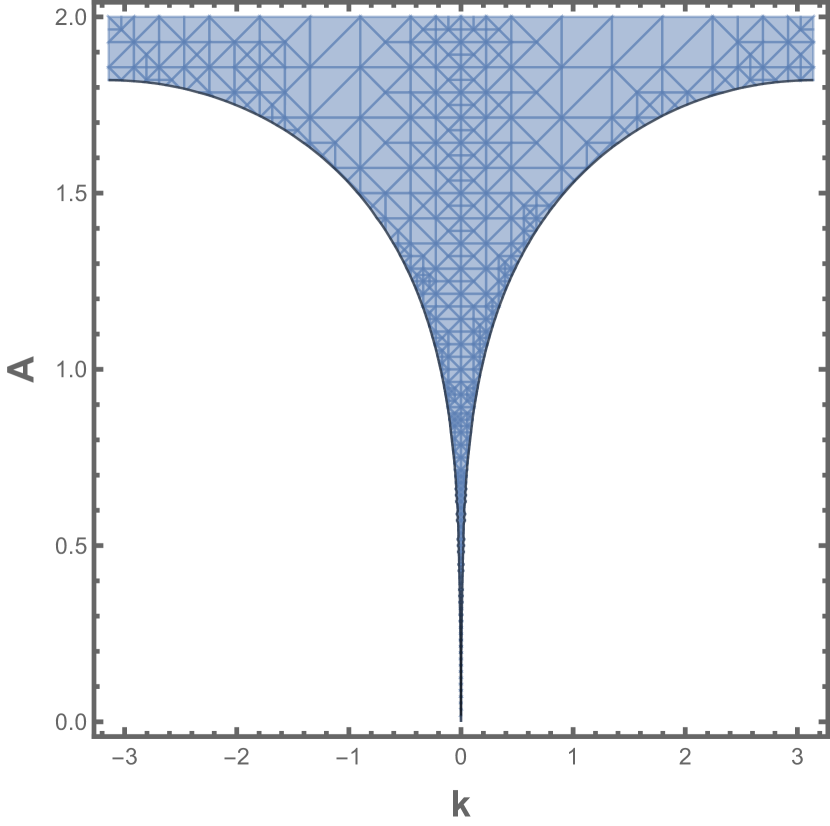
(a) $\alpha=0.5$

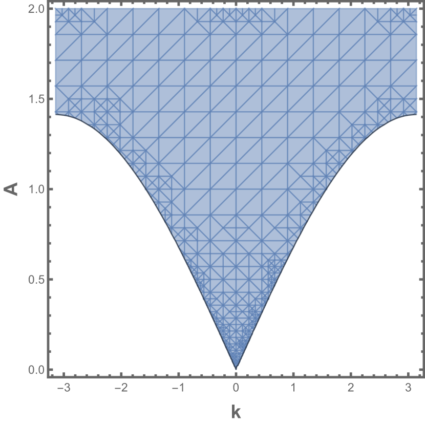
(b) $\alpha=50$

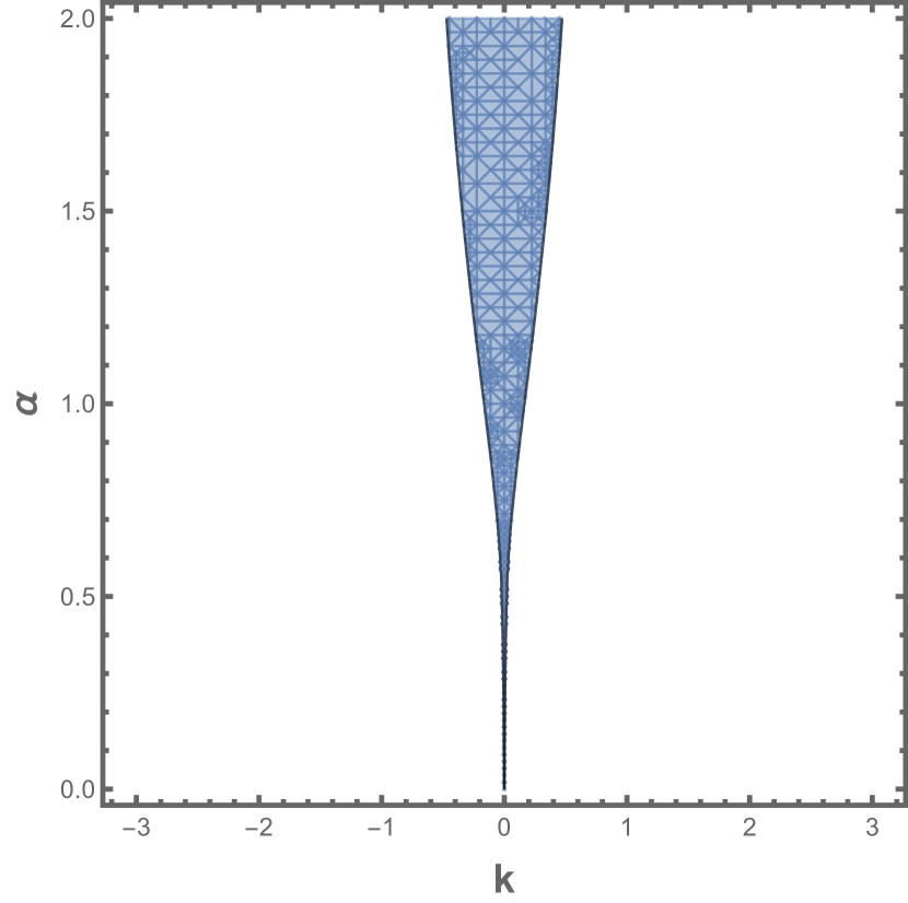
(c) $A=0.5$

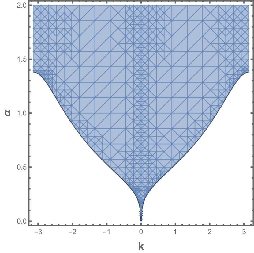
(d) $A=1.5$

Figure 1: Instability regions (blue) for $J_{n}=n^{-(1+\alpha)}$ in the $(k,A)$-plane and $(k,\alpha)$-plane where $k\in[-\pi,\pi]$ and $\epsilon=1$.

Proof.

The $\mathcal{O}(\mu)$ expansion yields

$$i\partial_{t}v_{n}=\epsilon\mathscr{L}_{\alpha}v_{n}-A^{2}(v_{n}+\overline{v_{n}}),$$ (4.1)

and setting $v_{n}=f_{n}+ig_{n}:=\Re v_{n}+i\Im v_{n}$, (4.1) is equivalent to

$$\frac{d}{dt}\begin{pmatrix}f_{n}\\ g_{n}\end{pmatrix}=\begin{pmatrix}0&\epsilon\mathscr{L}_{\alpha}\\ -\epsilon\mathscr{L}_{\alpha}+2A^{2}&0\end{pmatrix}\begin{pmatrix}f_{n}\\ g_{n}\end{pmatrix}.$$ (4.2)

Taking the Fourier transform $F(k,t)=\mathcal{F}[f_{n}(t)](k),\ G(k,t)=\mathcal{F}[g_{n}(t)](k)$ and the ansatz

$$\begin{pmatrix}F\\ G\end{pmatrix}=\begin{pmatrix}P(k)\\ Q(k)\end{pmatrix}e^{-i\Omega t},$$

(4.2) reduces to

$$\begin{pmatrix}i\Omega&2\epsilon\sum\limits_{m=1}J_{m}(1-\cos km)\\ -\left(2\epsilon\sum\limits_{m=1}J_{m}(1-\cos km)-2A^{2}\right)&i\Omega\end{pmatrix}\begin{pmatrix}P\\ Q\end{pmatrix}=\begin{pmatrix}0\\ 0\end{pmatrix},$$ (4.3)

where a nontrivial solution to (4.3) exists if and only if $\Omega$ satisfies the dispersion relation

$$\Omega^{2}=4\left(\epsilon\sum_{m=1}^{\infty}J_{m}(1-\cos(km))\right)\left(\epsilon\sum_{m=1}^{\infty}J_{m}(1-\cos(km))-A^{2}\right).$$ (4.4)

The frequency $\Omega$ is purely imaginary if and only if $\epsilon\sum\limits_{m=1}^{\infty}J_{m}(1-\cos(km))<A^{2}$, leading to modulational instability.

Suppose $\Phi=0$ and note that $\partial_{A}\Phi=-2A$. Since $A=0$ if and only if $k=0$, $A(k,\alpha,\epsilon)$ is analytic whenever $k\neq 0$ by the analytic Implicit Function Theorem. In the neighborhood of $k=0$, [38, Lemma A.1] implies that there exists $C(\alpha)>0$ such that

$$\frac{A^{2}}{\epsilon C\delta(k)}=\frac{A^{2}}{\epsilon C\delta(k)}\cdot\frac{\sum\limits_{m=1}^{\infty}J_{m}(1-\cos(km))}{\sum\limits_{m=1}^{\infty}J_{m}(1-\cos(km))}=\frac{\sum\limits_{m=1}^{\infty}J_{m}(1-\cos(km))}{C\delta(k)}\xrightarrow[k\rightarrow 0]{}1.$$

∎

When $J_{n}=n^{-(1+\alpha)}$, Figure 1 shows the region of instability. Note the non-analytic dependence of $A,\alpha$ on $k$ near the zero wavenumber. The instability region expands for bigger values of $A$, which is consistent with the $-A^{2}$ term in (4.4).

To compute the value(s) of $k\in[-\pi,\pi]$ that maximizes the exponential gain of the modulational instability, the RHS of (4.4) needs to be minimized under the condition $\Phi<0$; that a minimum exists follows from the Extreme Value Theorem since $\Omega(k)^{2}$ is continuous by the definition of $(J_{n})_{n=1}^{\infty}$. An explicit computation that minimizes $\Omega(k)^{2}$ is shown for a specific interaction kernel.

Figure 2: $k_{max}$ as a function of $\alpha$ when $J_{n}=n^{-(1+\alpha)}$. The values $A=1,\epsilon=1$ are used to generate this plot. For such parameters, $A_{0}\geq 2>A$ where $A_{0}$ is defined in Corollary 4.1, and therefore (4.5) is used to solve $k_{max}$ in $\alpha$. Observe that small $\alpha$ gives small $k_{max}$, manifested in the top left plot of Figure 3. That $k_{max}$ has an upper bound is numerically verified in Figure 3 for increasing values of $\alpha$.

Corollary 4.1.

For $\alpha,\epsilon>0$, let $J_{n}=n^{-(1+\alpha)},\ \tilde{w}(k)=\sum\limits_{m=1}^{\infty}\frac{1-\cos km}{m^{1+\alpha}},$ and $A_{0}:=\left(4\epsilon(1-2^{-(1+\alpha)})\zeta(1+\alpha)\right)^{\frac{1}{2}}$. Then for any $A\geq A_{0}$,

$$\min_{k\in[-\pi,\pi]}\Omega(k)^{2}=\Omega(\pm\pi)^{2}=-A_{0}^{2}(2A^{2}-A_{0}^{2}),$$

and if $0<A<A_{0}$, then there exists a unique $k_{max}\in(0,\pi)$ that minimizes $\Omega^{2}$ where $k_{max}$ satisfies

$$\tilde{w}(k_{max})=\frac{A^{2}}{2\epsilon}$$ (4.5)

and

$$\min_{k\in[-\pi,\pi]}\Omega(k)^{2}=\Omega(\pm k_{max})^{2}=-A^{4}.$$

Proof.

Since $\Omega(k)^{2}$ is even and $\Omega(0)=0$, let $k\in(0,\pi]$ without loss of generality. By direct computation, it can be shown that $\tilde{w}(0)=0,\ \tilde{w}\in C^{1}(0,\pi)$, and $\tilde{w}$ is increasing on $(0,\pi)$. From the derivative, we have

$$\begin{split}\frac{d}{dk}\left(\Omega(k)^{2}\right)&=4\epsilon\frac{d}{dk}\tilde{w}(k)\left(2\epsilon\overset{\sim}{w}(k)-A^{2}\right),\end{split}$$

and therefore $\Omega^{2}$ is decreasing if and only if $2\epsilon\tilde{w}(k)-A^{2}\leq 0$. Since

$$\max_{k\in[-\pi,\pi]}\tilde{w}(k)=\tilde{w}(\pm\pi)=\sum_{m\geq 1,\ m\ \text{odd}}\frac{2}{m^{1+\alpha}}=2(1-2^{-(1+\alpha)})\zeta(1+\alpha),$$ (4.6)

if $A\geq A_{0}$, then $2\epsilon\tilde{w}(k)-A^{2}\leq 0$ for all $k\in(0,\pi]$. Hence $\Omega^{2}$ is minimized at $k=\pm\pi$ and the value of $\Omega(\pm\pi)^{2}$ follows from (4.6). If $0<A<A_{0}$, then there exists a unique $k_{max}\in(0,\pi)$ satisfying $\tilde{w}(k_{max})=\frac{A^{2}}{2\epsilon}$ by the Intermediate Value Theorem and

$$\Omega(k_{max})^{2}=4\epsilon\tilde{w}(k_{max})\left(\epsilon\tilde{w}(k_{max})-A^{2}\right)=-A^{4}.$$

∎

What dynamics emerges after the initial linear growth due to MI is a question that has been posed since the studies of the FPUT chain. Based on many studies in discrete and continuous models, it is expected that the discrete modulational instability is the potential mechanism for the formation of nonlinear localized modes, such as discrete breathers and envelope solitons. What is not known is which type emerges in the fNLSE and what is the role of the parameter $\alpha$. Figure 3 shows a sample of emerging patterns triggered by numerical noise. While at this time we will not examine these emerging patterns, it is clear that $\alpha$-dependent coherent and robust patterns develop.

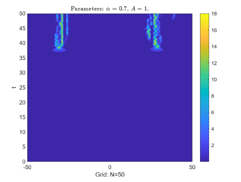
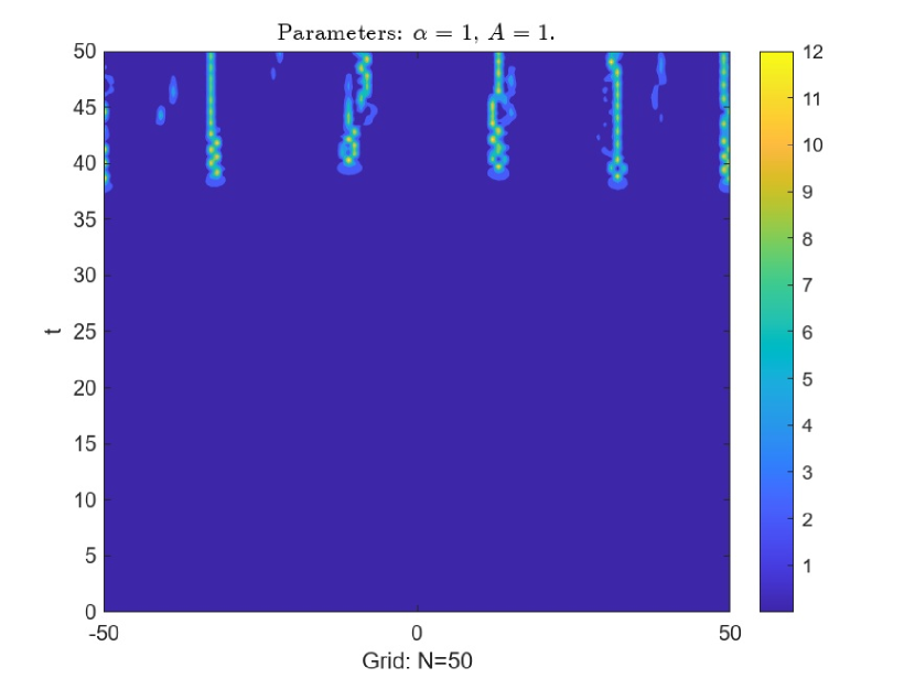
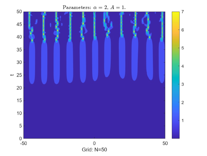
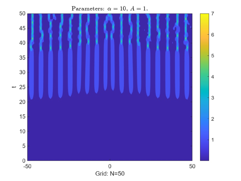
Figure 3: Emerging patterns triggered by numerical noise. Background intensity is the same in all cases, $A=1$ . The nonlinear state should be quasiperiodic, with an $\alpha$ dependence on the separation between peaks, likely to be close to the most unstable MI wavenumber $k_{max}$.

5 Asymptotic Construction of Stationary Solutions.

An important class of solutions for nonlinear coupled oscillators, are localized states carrying finite energy. It is expected as shown in the previous section, that stable localized modes are indeed coherent structures the system selects to allocate energy. Generically, there are no known analytic solutions, so typically one relies on numerical or asymptotic approximations. In order to highlight similarities and differences between the local and nonlocal coupling, we include known results from the DNLS. In one dimensional arrays, solutions are onsite if their intensity is centered at a grid site, and offsite if centered between two consecutive grid sites. To avoid confusions in notation, we denote $q_{n}$ by the onsite solution (mode $A$) satisfying $q_{n}=q_{-n}$ and $g_{n}$, the offsite solution (mode $B$) satisfying $g_{n}=g_{-(n-1)}$.

In Section 5.1, the stationary equation of DNLS is recasted as a discrete recurrence relation similar to [12, Chapter 11]. In Section 5.3 where the interaction kernel is of long range, the recurrence relation does not define a Markov chain; instead the forward map depends on all previous iterates and the phase space of solutions is infinite dimensional. Our asymptotic method has a disadvantage that the orbit of the recurrence relation does not give an exact solution, but has the advantage that it yields a localized sequence that satisfies the stationary equation in an appropriate limit.

5.1 Localized Solutions for DNLS.

We revisit the derivation of stationary solutions in [22, Section II] while relaxing the hypotheses that $\mathrm{supp}\{q_{n}\}$ and $\mathrm{supp}\{g_{n}\}$ are compact. To motivate Proposition 5.1, consider (2.3) with $J_{n}=1$, if $n=1$, and $J_{n}=0$ otherwise (nearest-neighbor coupling). Assume $q_{n}\geq 0$ and $q_{n+1}\ll q_{n}$ for all $n\geq 0$; see Proposition 5.1 for a precise statement. Neglecting $q_{\pm 1}$ yields

$$wq_{0}=-2\epsilon q_{0}+q_{0}^{3},$$

and therefore $q_{0}=\sqrt{w+2\epsilon}$. For $n\geq 1$, further assume $q_{n}\ll 1$, after which (2.3) neglecting $q_{n+1}$ and the nonlinear term yields

$$wq_{n}=\epsilon(q_{n-1}-2q_{n}),$$

and therefore $q_{n}=\frac{\epsilon}{(w+2\epsilon)}q_{n-1}$. By this method, a forward map is defined where $q_{n}$ depends on $q_{n-1}$. A similar computation can be done with $\{g_{n}\}$. This explicit construction yields a sequence in $l^{2}(\mathbb{Z})$ that satisfies (1.3) asymptotically as $\rho:=\frac{\epsilon}{w}\rightarrow 0$.

Proposition 5.1.

For $w,\epsilon>0$, let $\{q_{n}\}$ satisfy

$$q_{n}=\left(\frac{\epsilon}{w+2\epsilon}\right)^{|n|}\sqrt{w+2\epsilon},\ n\in\mathbb{Z}.$$ (5.1)

Then $q_{n+1}=o(q_{n})$ as $\rho:=\frac{\epsilon}{w}\rightarrow 0$. Moreover $\{q_{n}\}$ satisfies (2.3), with the nearest-neighbor coupling, asymptotically as $\rho\rightarrow 0$ uniformly in $n\in\mathbb{Z}$, or more precisely,

$$\lim_{\rho\rightarrow 0}\sup_{n\in\mathbb{Z}}\left|\frac{wq_{n}}{\epsilon(q_{n+1}+q_{n-1}-2q_{n})+q_{n}^{3}}-1\right|=0.$$ (5.2)

Proof.

By symmetry, let $n\geq 0$. An explicit computation yields,

$$\frac{q_{n+1}}{q_{n}}=\frac{\rho}{1+2\rho}\xrightarrow[\rho\rightarrow 0]{}0,$$

and

$$\frac{wq_{n}}{\epsilon(q_{n+1}+q_{n-1}-2q_{n})+q_{n}^{3}}=\begin{cases}\frac{1}{1+\rho^{2}(1+2\rho)^{-1}+\rho^{2n}(1+2\rho)^{1-2n}},\ n>0,\\ \frac{1}{1+2\rho^{2}(1+2\rho)^{-1}},\ n=0.\end{cases}$$ (5.3)

Taking the limit of the RHS of (5.3) as $\rho\rightarrow 0$, (5.2) is shown. ∎

Remark 5.1.

For $n\geq 1$, define $\{g_{n}\}$ as

$$g_{n}=\left(\frac{\epsilon}{w+2\epsilon}\right)^{n-1}\sqrt{w+\epsilon},$$ (5.4)

and extend to $\mathbb{Z}$ by $g_{n}=g_{-(n-1)}$. Then $g_{n+1}=o(g_{n})$ as $\rho\rightarrow 0$ for all $n\geq 1$ and satisfies (5.2) with $q_{n}$ replaced by $g_{n}$.

5.2 Peierls-Nabarro Barrier for DNLS.

A direct computation via geometric series and (2.4) yields an explicit expression for $E_{DNLS}$.

Proposition 5.2.

Let $q_{n},g_{n}$ be given by (5.1), (5.4), respectively. Then,

$$\begin{split}E_{A}(\epsilon,w)&=\frac{\epsilon(w+\epsilon)(w+2\epsilon)}{w+3\epsilon}-\frac{(w+2\epsilon)^{2}((w+2\epsilon)^{4}+\epsilon^{4})}{4((w+2\epsilon)^{4}-\epsilon^{4})},\\ E_{B}(\epsilon,w)&=\frac{\epsilon(w+\epsilon)^{2}}{w+3\epsilon}-\frac{(w+\epsilon)^{2}}{2\left(1-\frac{\epsilon^{4}}{(w+2\epsilon)^{4}}\right)}.\end{split}$$ (5.5)

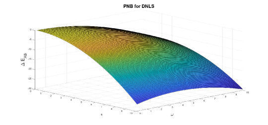
Figure 4: PNB for DNLS as a function of $\epsilon,w_{A}$. The numerical plot is consistent with Corollary 5.1 that there exists a unique local (and global) maximum at $(\epsilon^{*},w_{A}^{*})=(0,0)$.

Suppose $q_{n}$ oscillates in time at $w_{A}$ and $g_{n}$ at $w_{B}$. If $q_{n},g_{n}$ are two modes of the same traveling wave solution, then $N_{A}=N_{B}$. Since $N_{A}\sim w_{A},\ N_{B}\sim 2w_{B}$ for $w_{A},w_{B}\gg 1$, assume $w_{A}=2w_{B}$. As [22, Equation 9], the Peierls-Nabarro barrier is defined as the energy difference of the two modes at $w_{A},w_{B}$, respectively, which can be computed explicitly by (5.5). See Figure 4.

Corollary 5.1.

Let $\Delta E_{AB}=E_{A}(\epsilon,w_{A})-E_{B}(\epsilon,\frac{w_{A}}{2})$. Setting $\epsilon=kw_{A}$ for $k>0$, we have

$$\Delta E_{AB}=-\gamma(k)w_{A}^{2},$$

where $\gamma(k)$ is a strictly positive rational function satisfying $\gamma(k)\xrightarrow[k\rightarrow 0+]{}\frac{1}{8}$ and $\inf\limits_{k\geq 0}\gamma(k)>0$. Therefore $\Delta E_{AB}<0$ for any $\epsilon,w_{A}>0$ and $\lim\limits_{(\epsilon,w_{A})\rightarrow(\epsilon^{*},w_{A}^{*})}\Delta E_{AB}=0$ if and only if $(\epsilon^{*},w_{A}^{*})=(0,0)$. Furthermore as $w_{A}\rightarrow\infty$,

$$\Delta E_{AB}\sim_{\epsilon}-\frac{w_{A}^{2}}{8},\ \frac{E_{A}(\epsilon,w_{A})}{E_{B}(\epsilon,w_{B})}\sim_{\epsilon}2.$$

Remark 5.2.

As $h=\epsilon^{-\frac{1}{2}}\rightarrow 0$, we have $\Delta E_{AB}\sim-\frac{4}{15h^{4}}$ by direct computation via (5.5), which seems inconsistent with the exponential smallness of PNB

$$|\Delta E_{AB}|\lesssim(\sqrt{w}h)^{2-d}e^{-\frac{C}{\sqrt{w}h}},\ d=1,2,3,$$

that recovers the Galilean invariance of NLS as $h\rightarrow 0$; see [41, Theorem 3.3]. However, since $q_{n},g_{n}$ do not satisfy the DNLS asymptotically as $\epsilon\rightarrow\infty$, $\Delta E_{AB}$ for $\epsilon\gg 1$ given in Corollary 5.1, or equivalently $h\ll 1$ on $h\mathbb{Z}$, does not accurately describe the PNB.

5.3 Localized Solutions for fDNLS.

Localized on and offsite solutions for the fDNLS were studied in [9]. The authors correctly point out that the long-distance behavior of the intrinsically localized states depends on the rate of decay $1+\alpha$ and that as $\alpha$ gets larger, localization resembles that of the DNLS. As it relates to the asymptotic behavior ($n$ large), for the stationary solutions of

$$-\omega{q}_{n}=\epsilon\sum_{m\in\mathbb{Z}\setminus\{n\}}\frac{q_{n}-q_{m}}{|n-m|^{1+\alpha}}-q_{n}^{3},\ (n,t)\in\mathbb{Z}\times\mathbb{R},\ \epsilon>0,\ \alpha>0,$$

and using the Green’s function ($G_{n-m}$) formalism so that $q_{n}=\sum_{m}G_{n-m}q_{m}^{3}$, the authors in [9] conclude that the tail of the mode decays algebraically if $2<1+\alpha<3$ and exponentially in $n$ for $1+\alpha>3$. Our approach is different and instead we show below that in fact in all instances the tail decays algebraically.

Define

$$q_{0}=\sqrt{w+2\epsilon J},\ q_{n}=\frac{\epsilon\left(J_{n}q_{0}+\sum\limits_{m=1}^{n-1}\left(J_{n-m}+J_{n+m}\right)q_{m}\right)}{\epsilon\left(2J-J_{2n}\right)+w}, n\geq 1$$ (5.6a)

$$g_{0}=\sqrt{w+\epsilon(2J-J_{1})},\ g_{n}=\frac{\epsilon\sum\limits_{m=1}^{n-1}\left(J_{n-m}+J_{n+m-1}\right)g_{m}}{\epsilon\left(2J-J_{2n-1}\right)+w}, n\geq 2$$ . (5.6b)

To provide an insight for the definitions above, the first two terms of $q_{n}$ are shown explicitly. For $q_{0}$, neglect $q_{n}$ for $|n|\geq 1$. Then

$$-wq_{0}=2\epsilon Jq_{0}-q_{0}^{3},$$

and hence $q_{0}$. For $q_{1}$, neglect the nonlinear term $q_{1}^{3}$ and $q_{n}$ where $|n|\geq 2$. Since $q_{1}=q_{-1}$,

$$-wq_{1}=\epsilon\sum_{m\neq 1}J_{|1-m|}(q_{1}-q_{m})=2\epsilon Jq_{1}-\epsilon\left(J_{1}q_{0}+J_{2}q_{1}\right),$$

and so follows $q_{1}$. Although the analytic description of the asymptotic sequences is not immediately tractable, they are given by the power series expansion in the high-frequency regime.

Proposition 5.3.

Let $\rho=\frac{\epsilon}{w}$ and $0<\rho<\frac{1}{2J}$. Then there exist sequences $\{c_{nk}\}_{k\geq 1},\{d_{nk}\}_{k\geq 1}\subseteq\mathbb{R}$ such that

$$\begin{split}\frac{q_{n}}{q_{0}}&=\sum_{k=1}^{\infty}c_{nk}\rho^{k},\ n\geq 1\\ \frac{g_{n}}{g_{0}}&=\sum_{k=1}^{\infty}d_{nk}\rho^{k},\ n\geq 2,\end{split}$$ (5.7)

where the series are absolutely convergent and $c_{n1}=J_{n},\ d_{n1}=J_{n-1}+J_{n}$.

Proof.

For brevity, our proof concerns $q_{n}$ only. Let

$$\gamma_{n}=\frac{\rho}{1+\rho(2J-J_{2n})}.$$

Since $\rho$ is sufficiently small by hypothesis, $\gamma_{n}=\rho+O_{\alpha}(\rho^{2})$ by series expansion where the error term is uniform in $n$ since $|\rho(2J-J_{2n})|<2\rho J<1$. Let $n=1$. From (5.6a),

$$\frac{q_{1}}{q_{0}}=\gamma_{1}J_{1}=\frac{\rho J_{1}}{1+\rho(2J-J_{1})},$$

and hence (5.7) with $c_{n1}=J_{1}$. Suppose the claim holds for $m=1,\dots,n-1$. Then

$$\frac{q_{n}}{q_{0}} =\gamma_{n}J_{n}+\gamma_{n}\sum\limits_{m=1}^{n-1}\left(J_{n-m}+J_{n+m}\right)\frac{q_{m}}{q_{0}}$$

$$=\gamma_{n}J_{n}+\gamma_{n}\sum_{k=1}^{\infty}\sum_{m=1}^{n-1}\left(J_{n-m}+J_{n+m}\right)c_{mk}\rho^{k},$$ (5.8)

where the series is absolutely convergent since

$$\sum_{k=1}^{\infty}\sum_{m=1}^{n-1}\left(J_{n-m}+J_{n+m}\right)|c_{mk}|\rho^{k}\leq J\cdot\max_{1\leq m\leq n-1}\left(\sum_{k=1}^{\infty}|c_{mk}|\rho^{k}\right)<\infty.$$

The second term of (5.3) is $O(\rho^{2})$, and hence the dominant term of $\frac{q_{n}}{q_{0}}$ is $\rho J_{n}$. ∎

By Proposition 5.3,

$$\left|\frac{q_{n}/q_{0}}{\rho J_{n}}-1\right|=J_{n}^{-1}\left|\sum_{k=2}^{\infty}c_{nk}\rho^{k-1}\right|\xrightarrow[\rho\rightarrow 0]{}0,$$

and hence for any $n\in\mathbb{Z}\setminus\{0\}$,

$$\frac{q_{n}}{q_{0}}\sim\rho J_{n},\ \rho\rightarrow 0.$$ (5.9)

In fact, the convergence rate of (5.9) is uniform in $n$.

Proposition 5.4.

For all $\epsilon_{1},\alpha>0$, there exists $\rho_{*}=\rho_{*}(\epsilon_{1},\alpha)>0$ such that for any $0<\rho<\rho_{*}$,

$$\begin{split}\frac{1}{1+\epsilon_{1}}&<\frac{q_{n}/q_{0}}{\rho J_{n}}<1+\epsilon_{1},\ n\geq 1,\\ \frac{1}{1+\epsilon_{1}}&\leq\frac{g_{n}/g_{0}}{\rho(J_{n}+J_{n-1})}\leq 1+\epsilon_{1},\ n\geq 2.\end{split}$$ (5.10)

Proof.

The proof is for $q_{n}$ without loss of generality. Since $n^{1+\alpha}J_{n}\xrightarrow[n\rightarrow\infty]{}A$, there exists $N\in\mathbb{N}$ such that for any $n\geq N$, we have $|J_{n}-\frac{A}{n^{1+\alpha}}|<\frac{A}{2n^{1+\alpha}}$. Define

$$\rho_{*}=\min\left(\frac{\epsilon_{1}}{2J},\min\limits_{2\leq n\leq 2N}\left(\frac{\epsilon_{1}J_{n}}{2(1+\epsilon_{1})(n-1)J^{2}}\right),\frac{\epsilon_{1}}{3(1+2^{2+\alpha})(1+\epsilon_{1})J}\right).$$

By (5.6a),

$$\frac{q_{n}}{q_{0}}\geq\gamma_{n}J_{n}>\frac{\rho J_{n}}{1+2\rho J}>\frac{\rho J_{n}}{1+\epsilon_{1}},$$

and hence the lower bound of (5.10). The proof for the upper bound is by induction. For the base case, we have

$$\frac{q_{1}}{\rho J_{1}q_{0}}=\frac{1}{1+\rho(2J-J_{2})}<1+\epsilon_{1}.$$

Let $C=(1+\epsilon_{1})\rho q_{0}$. For $2\leq n\leq 2N$,

$$q_{n}<\rho\left(J_{n}q_{0}+C\sum_{m=1}^{n-1}(J_{n-m}+J_{n+m})J_{m}\right)\leq\rho\left(J_{n}q_{0}+2C(n-1)J^{2}\right)<CJ_{n},$$

since $\rho<\rho_{*}$.

Let $n>2N$. Suppose $q_{m}<CJ_{m}$ for all $1\leq m\leq n-1$. Observe that

$$\begin{split}\sum_{m=1}^{n-1}J_{n-m}q_{m}&<C\left(\sum_{1\leq m\leq\frac{n}{2}}J_{n-m}J_{m}+\sum_{\frac{n}{2}<m\leq n-1}J_{n-m}J_{m}\right)\\ &<\frac{3CA}{2}\left(\sum_{1\leq m\leq\frac{n}{2}}\frac{J_{m}}{(n-m)^{1+\alpha}}+\sum_{\frac{n}{2}<m\leq n-1}\frac{J_{n-m}}{m^{1+\alpha}}\right)\\ &\leq 3\cdot 2^{1+\alpha}CAn^{-(1+\alpha)}J<3\cdot 2^{2+\alpha}CJJ_{n}.\end{split}$$

A similar computation yields

$$\sum_{m=1}^{n-1}J_{n+m}q_{m}<3CJJ_{n},$$

and altogether,

$$q_{n}<\rho\left(q_{0}+3(1+2^{2+\alpha})CJ\right)J_{n}<CJ_{n}.$$

This completes the induction, and the claim for $g_{n}$ follows similarly. ∎

Corollary 5.2.

Assuming the hypotheses of Proposition 5.4,

$$\frac{q_{n}}{q_{0}}\sim\frac{A\rho}{n^{1+\alpha}},\hskip 20.0pt\frac{q_{n+1}}{q_{n}}\sim\left(\frac{n}{n+1}\right)^{1+\alpha},\hskip 20.0pt\frac{q_{2n}}{q_{n}}\sim 2^{-(1+\alpha)},$$

as $\rho\rightarrow 0$ and $n\rightarrow\infty$, and similarly for $\{g_{n}\}$.

As Proposition 5.1, it is shown that (5.6a), (5.6b) solve (2.3) in an asymptotic sense.

Proposition 5.5.

For any $\epsilon,w,\alpha>0$, define $\{q_{n}\}$ by (5.6a). Then $q_{n+1}=O(q_{n})$ as $\rho\rightarrow 0$, and

$$\lim_{\rho\rightarrow 0}\sup_{n\in\mathbb{Z}}\left|\frac{-wq_{n}}{\epsilon\mathscr{L}_{\alpha}q_{n}-q_{n}^{3}}-1\right|=0,$$ (5.11)

and similarly for $\{g_{n}\}$.

Proof.

The big-O bound follows from Corollary 5.2. The proof is for $q_{n}$ and $n\geq 1$. By Proposition 5.4,

$$-wq_{n}\sim-w\rho J_{n}q_{0}=-w^{\frac{3}{2}}\rho J_{n}(1+2\rho J)^{\frac{1}{2}}.$$

The interaction term is given by

$$\epsilon\sum_{m\neq n}J_{|n-m|}(q_{n}-q_{m})=\epsilon J_{n}(q_{n}-q_{0})+\epsilon\sum_{m\notin\{0,n\}}J_{|n-m|}(q_{n}-q_{m})=:I+II,$$

and estimating the terms separately, we have

$$I\sim-\epsilon J_{n}q_{0}=-w^{\frac{3}{2}}\rho J_{n}(1+2\rho J)^{\frac{1}{2}},$$

and

$$II\sim\epsilon\rho q_{0}\sum_{m\notin\{0,n\}}J_{|n-m|}(J_{|n|}-J_{|m|})\leq 2w^{\frac{3}{2}}\rho^{2}(1+2\rho J)^{\frac{1}{2}}J^{2}.$$ (5.12)

It follows that $II$ is $O(\rho^{2})$ and hence negligible. So is the nonlinear term, which is $O(w^{\frac{3}{2}}\rho^{3})$. The uniformity in $n$ follows as Corollary 5.2. The limit (5.11) can be shown similarly for the case $n=0$. ∎

5.4 Peierls-Nabarro Barrier for fDNLS.

In this part, we assume $J_{n}=n^{-(1+\alpha)}$. The PNB for fDNLS is fundamentally different from that of the nearest-neighbor interaction. The PNB can take both positive and negative values, and it can increase in $\epsilon$ or $w$ depending on $\alpha$; see Figures 4 and 5. This suggests that the onsite solution need not always be the energy minimizer of the Hamiltonian. It is of interest to further investigate the role of non-locality in the framework of variational approach to fDNLS and the stability properties of onsite/offsite solutions. By (2.4) and the symmetry properties of the onsite/offsite solutions, an analogue of Proposition 5.2 is derived. The proof follows from Corollary 5.2 and standard algebra, and thus is omitted.

Proposition 5.6.

Let $q_{n},g_{n}$ be given by (5.6a), (5.6b), respectively. Then,

$$\begin{split}E_{A}&=\epsilon\sum_{n=1}^{\infty}\Biggl{(}\frac{|q_{n}-q_{0}|^{2}}{n^{1+\alpha}}+\frac{1}{2}\sum_{\begin{subarray}{c}m=1\\ m\neq n\end{subarray}}^{\infty}\left(\frac{1}{|n-m|^{1+\alpha}}+\frac{1}{|n+m|^{1+\alpha}}\right)|q_{n}-q_{m}|^{2}\Biggl{)}-\left(\frac{1}{4}q_{0}^{4}+\frac{1}{2}\sum_{n=1}^{\infty}q_{n}^{4}\right),\\ E_{B}&=\epsilon\sum_{n=2}^{\infty}\Biggl{(}\left(\frac{1}{n^{1+\alpha}}+\frac{1}{(n-1)^{1+\alpha}}\right)|g_{n}-g_{0}|^{2}\\ &\hskip 120.0pt+\frac{1}{2}\sum_{\begin{subarray}{c}m=2\\ m\neq n\end{subarray}}^{\infty}\left(\frac{1}{|n-m|^{1+\alpha}}+\frac{1}{|n+m-1|^{1+\alpha}}\right)|g_{n}-g_{m}|^{2}\Biggl{)}-\frac{1}{2}\sum_{n=1}^{\infty}g_{n}^{4}.\end{split}$$ (5.13)

The analysis in Section 5.3 was simplified under the assumption $\rho=\frac{\epsilon}{w}\ll 1$. A similar analysis is further developed in the context of PNB using Proposition 5.6. By the conservation of particle number, assume $w_{A}=2w_{B}$.

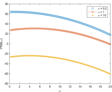
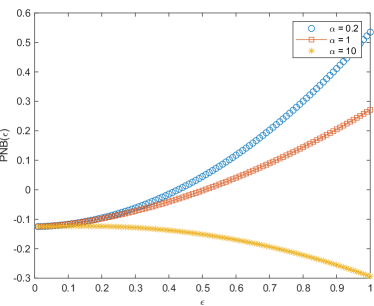
Figure 5: The left plot ($\epsilon=10$) shows the transient state of PNB($\omega$) before they converge to $-\frac{w_{A}^{2}}{8}$ as $w_{A}\rightarrow\infty$. The right plot ($w=1$) shows the PNB diverging away from $-\frac{w_{A}^{2}}{8}$, the initial value at $\epsilon=0$, as $\epsilon>0$ increases.

Corollary 5.3.

As $w_{A},w_{B}\rightarrow\infty$,

$$\begin{split}E_{A}&\sim-\frac{w_{A}^{2}}{4}-(2\zeta(2+2\alpha)+\zeta(1+\alpha)^{2})\epsilon^{2},\\ E_{B}&\sim-\frac{w_{B}^{2}}{2}-\left(2\sum_{n=2}^{\infty}\left(\frac{1}{n^{1+\alpha}}+\frac{1}{(n-1)^{1+\alpha}}\right)^{2}+\frac{1}{2}(2\zeta(1+\alpha)-1)^{2}\right)\epsilon^{2}.\end{split}$$

Therefore, $E_{A}(w_{A})\sim 2E_{B}(w_{B})$ and

$$\Delta E_{AB}\sim-\frac{w_{A}^{2}}{8}.$$

Corollary 5.4.

As $\epsilon\rightarrow 0$,

$$\begin{split}E_{A}&\sim-\frac{w_{A}^{2}}{4}+\left(-2\zeta(2+2\alpha)+\zeta(1+\alpha)^{2}\right)\epsilon^{2},\\ E_{B}&\sim-\frac{w_{B}^{2}}{2}+\left(-2\sum_{n=2}^{\infty}\left(\frac{1}{n^{1+\alpha}}+\frac{1}{(n-1)^{1+\alpha}}\right)^{2}+\frac{1}{2}(2\zeta(1+\alpha)-1)^{2}\right)\epsilon^{2}.\end{split}$$

Therefore, $E_{A}(w_{A})\sim 2E_{B}(w_{B})$ and

$$\Delta E_{AB}\sim-\frac{w_{A}^{2}}{8}+\left(2\sum_{n=2}^{\infty}\left(\frac{1}{n^{1+\alpha}}+\frac{1}{(n-1)^{1+\alpha}}\right)^{2}-(\zeta(1+\alpha)-1)^{2}-2\zeta(2+2\alpha)+\frac{1}{2}\right)\epsilon^{2}.$$

For $w_{A}>0$ not sufficiently large, $PNB(w_{A})$ may not be well approximated by the quadratic term; in fact, $PNB(w_{A})$ may be increasing for $w_{A}>0$ sufficiently small. For $\epsilon>0$ not sufficiently small, the behavior of PNB is generally not quadratic in $\epsilon$ since the higher order terms cannot be neglected. For $\epsilon\ll 1$, note that PNB may increase or decrease depending on the sign of the coefficient of $\epsilon^{2}$.

Remark 5.3.

As $\alpha\rightarrow 0$, or more precisely, for $\alpha\ll\min(1,\frac{\epsilon}{w})$, observe that $\frac{1}{\alpha}<\zeta(1+\alpha)<1+\frac{1}{\alpha}$ yields

$$N_{A}\sim q_{0}^{2}\sim\frac{2\epsilon}{\alpha},\ N_{B}\sim 2g_{0}^{2}\sim\frac{4\epsilon}{\alpha}.$$

Since $N_{B}\sim 2N_{A}$, the conservation of particle number as a localized wave travels along the lattice in the forms of onsite and offsite waves, if such solutions exist at all, does not hold. This suggests that the PNB for small $\alpha>0$ calculated from (5.13) is non-physical.

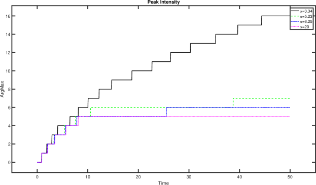
Figure 6: Position of peak intensity for traveling waves of the fDNLS for $\epsilon=1,w=1$, $v=1$ and varying $\alpha\in\{3.34,5.23,6.25,20\}$.

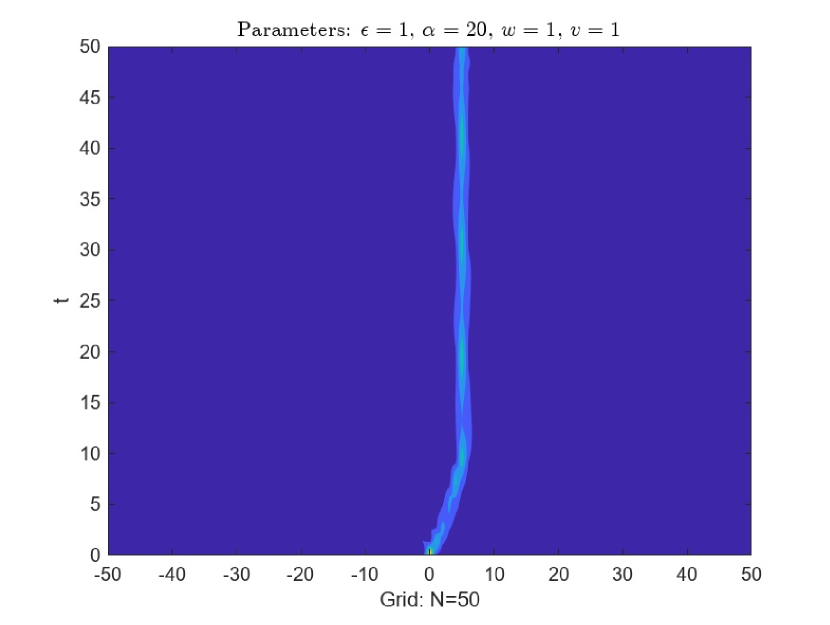
Figure 7: Intensity plots for varying $\alpha\in\{0.3,3.34,5,20\}$. The top-left plot illustrates the log intensity.

In Figures 6 and 7, the mobility/pinning of peak intensity is observed in the nonlocal dynamics given by $J_{n}=|n|^{-(1+\alpha)}$ for $n\neq 0$ with the initial condition as the onsite sequence defined in (5.6a). As $\alpha\rightarrow 0$, the nonlocal coupling blows up as $\lim\limits_{\alpha\rightarrow 0+}\zeta(1+\alpha)=\infty$. Moreover the conservation of particle numbers between the onsite and offsite solutions fails in the sense described in Remark 5.3, resulting in the erratic behavior illustrated in the top-left plot of Figure 7. For $\alpha$ not too small, the intensity drifts and eventually pins at a lattice point. More precisely as $\alpha\to\infty$, the non-locality weakens, leading to a weaker drift (pinning) at earlier times. See [42, Figure 1] for the drift and pinning under the DNLS dynamics for varying mesh grid sizes $h>0$ whereas Figure 6 plots the argmax of peak intensity for various $\alpha$.

6 Conclusion

The study of existence, dynamics and interactions of coherent, localized structures in nonlinear lattices remains an active field given the wide range of applications. Here we presented work for a model where the coupling between units (oscillators, waveguides, resonators) of a one dimensional arrays is global, with strength decaying algebraically with respect to the index difference. Results include the characterization of modulational instability and emergence of nonlinear modes for large times, obtained by numerical simulations. By use of asymptotic techniques we show the existence of localized modes and to assess mobility, derived formulas for the Peierls-Nabarro barrier. In all instances we point to the behavior in terms of the coupling strength parameter $\alpha$. This parametric dependece of the dynamics can have potential applications. Future work will further explore these applications, extend work to consider interaction properties (collisions) between localized modes. Finally, there are two natural extensions of this work; first the study of two-dimensional lattices with similar coupling functionality and second is for the long wave limit, to identify the continuum limit.

7 Acknowledgements

Both B.C. and A.M. acknowledge support from the NSF RTG award, DMS-1840260.

Appendix A Appendix

For our numerical simulations, a particular interaction kernel $J_{n}=|n|^{-(1+\alpha)}$ was used. Consider $(u_{n})$ for $n=-N,\dots,N$. Then for the Dirichlet boundary condition, we have

$$\mathscr{L}_{\alpha}u_{n}=\sum_{-N\leq m\leq N,m\neq n}\frac{u_{n}-u_{m}}{|n-m|^{1+\alpha}},$$ (A.1)

where $u_{m}=0$ for all $|m|>N$.

For the periodic boundary condition, consider the modular arithmetics where the quotient space of $\mathbb{Z}$, with $I_{N}:=\{-N,\dots,N-1\}$ as the fundamental cell, is considered, as $u_{-N}=u_{N}$. Given $m\in\mathbb{Z}$, let $m=2Nq+r$ where $q\in\mathbb{Z},\ r\in I_{N}$, and assume $u_{m}=u_{r}$. Then for $n\in I_{N}$,

$$\begin{split}\mathscr{L}_{\alpha}u_{n}&=\sum_{m\neq n}\frac{u_{n}-u_{m}}{|n-m|^{1+\alpha}}\\ &=2\zeta(1+\alpha)\left(1-\frac{1}{(2N)^{1+\alpha}}\right)u_{n}-\sum\limits_{r\neq n}c_{nr}(N,\alpha)u_{r},\end{split}$$ (A.2)

where

$$c_{nr}:=\frac{1}{|n-r|^{1+\alpha}}+\frac{1}{(2N)^{1+\alpha}}\bigg{\{}\zeta(1+\alpha,\frac{r-n}{2N})+\zeta(1+\alpha,-\frac{r-n}{2N})-|\frac{r-n}{2N}|^{-(1+\alpha)}(1+e^{-i(1+\alpha)\pi})\bigg{\}},$$ (A.3)

and $\zeta(s)=\sum\limits_{k=1}^{\infty}\frac{1}{k^{s}}$ is the Riemann zeta function and $\zeta(s,a)=\sum\limits_{k=0}^{\infty}\frac{1}{(k+a)^{s}}$ is the Hurwitz zeta function. Lastly we provide a brief derivation of (A.3). Using $m=2Nq+r$ as above,

$$\begin{split}\sum_{m\neq n}\frac{u_{n}-u_{m}}{|n-m|^{1+\alpha}}&=2\zeta(1+\alpha)u_{n}-\sum_{m\neq n}\frac{u_{m}}{|n-m|^{1+\alpha}}\\ &=2\zeta(1+\alpha)u_{n}-\sum_{r\in I_{N}\setminus\{n\}}\frac{u_{r}}{|n-r|^{1+\alpha}}-\sum_{r\in I_{N}}\sum_{q\in\mathbb{Z}\setminus\{0\}}\frac{u_{r}}{|q(2N)+r-n|^{1+\alpha}}\end{split}$$

The last sum simplifies to $2\zeta(1+\alpha)(2N)^{-(1+\alpha)}u_{n}$ when $r=n$. When $r\neq n$,

$$\begin{split}\sum_{q\in\mathbb{Z}\setminus\{0\}}\frac{(2N)^{1+\alpha}u_{r}}{|q(2N)+r-n|^{1+\alpha}}&=\sum_{q=1}^{\infty}\frac{1}{(q+\frac{r-n}{N})^{1+\alpha}}+\sum_{q=1}^{\infty}\frac{1}{(q-\frac{r-n}{N})^{1+\alpha}}\\ &=\zeta(1+\alpha,\frac{r-n}{N})+\zeta(1+\alpha,-\frac{r-n}{N})-|\frac{r-n}{N}|^{-(1+\alpha)}\left(1+e^{-i(1+\alpha)\pi}\right).\end{split}$$

Rearranging terms, the expression for $\mathscr{L}_{\alpha}u_{n}$ is derived as a matrix multiplication with dense entries.

References

- [1] H. Eisenberg, Y. Silberberg, R. Morandotti, A. Boyd, and J. Aitchison, “Discrete spatial optical solitons in waveguide arrays,” Physical Review Letters, vol. 81, no. 16, p. 3383, 1998.
- [2] R. Morandotti, U. Peschel, J. Aitchison, H. Eisenberg, and Y. Silberberg, “Dynamics of discrete solitons in optical waveguide arrays,” Physical Review Letters, vol. 83, no. 14, p. 2726, 1999.
- [3] A. Aceves, C. De Angelis, T. Peschel, R. Muschall, F. Lederer, S. Trillo, and S. Wabnitz, “Discrete self-trapping, soliton interactions, and beam steering in nonlinear waveguide arrays,” Physical Review E, vol. 53, no. 1, p. 1172, 1996.
- [4] B. P. Anderson and M. A. Kasevich, “Macroscopic quantum interference from atomic tunnel arrays,” Science, vol. 282, no. 5394, pp. 1686–1689, 1998.
- [5] G. Kalosakas, K. Rasmussen, and A. Bishop, “Delocalizing transition of bose-einstein condensates in optical lattices,” Physical review letters, vol. 89, no. 3, p. 030402, 2002.
- [6] A. Smerzi, S. Fantoni, S. Giovanazzi, and S. Shenoy, “Quantum coherent atomic tunneling between two trapped bose-einstein condensates,” Physical Review Letters, vol. 79, no. 25, p. 4950, 1997.
- [7] A. Trombettoni and A. Smerzi, “Discrete solitons and breathers with dilute bose-einstein condensates,” Physical Review Letters, vol. 86, no. 11, p. 2353, 2001.
- [8] S. F. Mingaleev, P. L. Christiansen, Y. Gaididei, M. Johansson, and K. Ø. Rasmussen, “Models for energy and charge transport and storage in biomolecules,” Journal of Biological Physics, vol. 25, pp. 41–63, Mar 1999.
- [9] Y. B. Gaididei, S. F. Mingaleev, P. L. Christiansen, and K. O. Rasmussen, “Effects of nonlocal dispersive interactions on self-trapping excitations,” Phys. Rev. E, vol. 55, pp. 6141–6150, May 1997.
- [10] D. S. Bassett and O. Sporns, “Network neuroscience,” Nature neuroscience, vol. 20, no. 3, pp. 353–364, 2017.
- [11] M. Rohden, A. Sorge, M. Timme, and D. Witthaut, “Self-organized synchronization in decentralized power grids,” Physical review letters, vol. 109, no. 6, p. 064101, 2012.
- [12] P. G. Kevrekidis, “The discrete nonlinear schrödinger equation.”
- [13] Y. S. Kivshar and G. P. Agrawal, Optical solitons: from fibers to photonic crystals. Academic press, 2003.
- [14] P.-L. S. Catherine Sulem, The Nonlinear Schrödinger Equation: Self-focusing and Wave Collapse. Applied Mathematical Sciences, Springer, 1 ed., 1999.
- [15] Y. V. Kartashov, B. A. Malomed, and L. Torner, “Solitons in nonlinear lattices,” Rev. Mod. Phys., vol. 83, pp. 247–305, Apr 2011.
- [16] M. I. Molina, “The two-dimensional fractional discrete nonlinear schrödinger equation,” Physics Letters A, vol. 384, no. 33, p. 126835, 2020.
- [17] M. Johansson, Y. B. Gaididei, P. L. Christiansen, and K. Rasmussen, “Switching between bistable states in a discrete nonlinear model with long-range dispersion,” Physical Review E, vol. 57, no. 4, p. 4739, 1998.
- [18] K. Rasmussen, P. L. Christiansen, M. Johansson, Y. B. Gaididei, and S. Mingaleev, “Localized excitations in discrete nonlinear schrödinger systems: effects of nonlocal dispersive interactions and noise,” Physica D: Nonlinear Phenomena, vol. 113, no. 2-4, pp. 134–151, 1998.
- [19] P. L. Christiansen, Y. B. Gaididei, F. G. Mertens, and S. F. Mingaleev, “Multi-component structure of nonlinear excitations in systems with length-scale competition,” The European Physical Journal B-Condensed Matter and Complex Systems, vol. 19, pp. 545–553, 2001.
- [20] N. Korabel and G. M. Zaslavsky, “Transition to chaos in discrete nonlinear schrödinger equation with long-range interaction,” Physica A: Statistical Mechanics and its Applications, vol. 378, no. 2, pp. 223–237, 2007.
- [21] S. Longhi, “Fractional schrödinger equation in optics,” Optics letters, vol. 40, no. 6, pp. 1117–1120, 2015.
- [22] Y. S. Kivshar and D. K. Campbell, “Peierls-nabarro potential barrier for highly localized nonlinear modes,” Phys. Rev. E, vol. 48, pp. 3077–3081, Oct 1993.
- [23] O. Bang and P. D. Miller, “Exploiting discreteness for switching in waveguide arrays,” Optics letters, vol. 21, no. 15, pp. 1105–1107, 1996.
- [24] M. I. Weinstein, “Nonlinear schrödinger equations and sharp interpolation estimates,” Communications in Mathematical Physics, vol. 87, pp. 567–576, 1983.
- [25] M. I. Weinstein, “The nonlinear schrödinger equation—singularity formation, stability and dispersion,” The Connection between Infinite Dimensional and Finite Dimensional Dynamical Systems, pp. 213–232, 1989.
- [26] V. Zakharov and L. Ostrovsky, “Modulation instability: The beginning,” Physica D: Nonlinear Phenomena, vol. 238, no. 5, pp. 540–548, 2009.
- [27] T. Dauxois and M. Peyrard, “Energy localization in nonlinear lattices,” Physical review letters, vol. 70, no. 25, p. 3935, 1993.
- [28] I. Daumont, T. Dauxois, and M. Peyrard, “Modulational instability: first step towards energy localization in nonlinear lattices,” Nonlinearity, vol. 10, no. 3, p. 617, 1997.
- [29] V. E. Zakharov, A. I. Dyachenko, and A. O. Prokofiev, “Freak waves as nonlinear stage of stokes wave modulation instability,” European Journal of Mechanics-B/Fluids, vol. 25, no. 5, pp. 677–692, 2006.
- [30] V. E. Zakharov and A. Gelash, “Nonlinear stage of modulation instability,” Physical review letters, vol. 111, no. 5, p. 054101, 2013.
- [31] A. Gelash, D. Agafontsev, V. Zakharov, G. El, S. Randoux, and P. Suret, “Bound state soliton gas dynamics underlying the spontaneous modulational instability,” Physical review letters, vol. 123, no. 23, p. 234102, 2019.
- [32] L. Zhang, Z. He, C. Conti, Z. Wang, Y. Hu, D. Lei, Y. Li, and D. Fan, “Modulational instability in fractional nonlinear schrödinger equation,” Communications in Nonlinear Science and Numerical Simulation, vol. 48, pp. 531–540, 2017.
- [33] A. Aceves and A. Copeland, “Spatiotemporal dynamics in the fractional nonlinear schrödinger equation,” Frontiers, Nonlinear Photonics, vol. 3, 2022.
- [34] V. D. Dinh, “Blow-up criteria for fractional nonlinear schrödinger equations,” Nonlinear Analysis: Real World Applications, vol. 48, pp. 117–140, 2019.
- [35] Y. Hong and Y. Sire, “On fractional schrödinger equations in sobolev spaces,” Communications on Pure & Applied Analysis, vol. 14, no. 6, pp. 2265–2282, 2015.
- [36] V. D. Dinh, “Well-posedness of nonlinear fractional Schrödinger and wave equations in Sobolev spaces,” International Journal of Applied Mathematics, vol. 31, pp. 483–525, Sept. 2018.
- [37] B. Choi and A. Aceves, “Well-posedness of the mixed-fractional nonlinear schrödinger equation on r2,” Partial Differential Equations in Applied Mathematics, vol. 6, p. 100406, 2022.
- [38] K. Kirkpatrick, E. Lenzmann, and G. Staffilani, “On the continuum limit for discrete nls with long-range lattice interactions,” Communications in mathematical physics, vol. 317, no. 3, pp. 563–591, 2013.
- [39] Y. Hong and C. Yang, “Strong convergence for discrete nonlinear schrödinger equations in the continuum limit,” SIAM Journal on Mathematical Analysis, vol. 51, no. 2, pp. 1297–1320, 2019.
- [40] B. Choi and A. Aceves, “Continuum limit of 2d fractional nonlinear schrödinger equation,” Journal of Evolution Equations, vol. 23, no. 2, p. 30, 2023.
- [41] M. Jenkinson and M. I. Weinstein, “On-site and off-site bound states of the discrete nonlinear schrödinger equation and the peierls-nabarro barrier,” 2014.
- [42] M. Jenkinson and M. I. Weinstein, “Discrete solitary waves in systems with nonlocal interactions and the peierls–nabarro barrier - communications in mathematical physics,” Feb 2017.
- [43] A. Lischke, G. Pang, M. Gulian, F. Song, C. Glusa, X. Zheng, Z. Mao, W. Cai, M. M. Meerschaert, M. Ainsworth, and G. E. Karniadakis, “What is the fractional laplacian?,” 2019.
- [44] M. I. Weinstein, “Excitation thresholds for nonlinear localized modes on lattices,” Nonlinearity, vol. 12, no. 3, p. 673, 1999.
- [45] A. Stefanov and P. G. Kevrekidis, “Asymptotic behaviour of small solutions for the discrete nonlinear schrödinger and klein–gordon equations,” Nonlinearity, vol. 18, no. 4, p. 1841, 2005.
- [46] E. M. Stein and T. S. Murphy, Harmonic analysis: real-variable methods, orthogonality, and oscillatory integrals, vol. 3. Princeton University Press, 1993.
- [47] M. Keel and T. Tao, “Endpoint strichartz estimates,” American Journal of Mathematics, vol. 120, no. 5, pp. 955–980, 1998.
- [48] T. Tao, Nonlinear dispersive equations: local and global analysis. No. 106, American Mathematical Soc., 2006.