Mesoscale modeling of deformations and defects in crystalline sheets

Abstract

We study deformations and defects in thin, flexible sheets with crystalline order using a coarse-grained Phase-Field Crystal (PFC) model. The PFC model describes crystals at diffusive timescales through a continuous periodic field representing the atomic number density. In its amplitude expansion (APFC), a coarse-grained description featuring slowly varying fields retaining lattice deformation, elasticity, and an advanced description of dislocations is achieved. We introduce surface PFC and APFC models in a convenient height formulation encoding normal deformation. With this framework, we then study general aspects of the buckling of strained sheets, defect nucleation on a prescribed deformed surface, and out-of-plane relaxation near dislocations. We benchmark and discuss our results by looking at the continuum limit for buckling under elastic deformation, and at evidence from microscopic models for deformation at defects and defect arrangements. We shed light on the fundamental interplay between lattice distortion at dislocations and out-of-plane deformation by looking at the effect of the annihilation of dislocation dipoles. The scale-bridging capabilities of the devised mesoscale framework are also showcased with the simulation of a representative thin sheet hosting many dislocations.

1 Introduction

Elastic films are ubiquitous in both natural and manufactured systems. They display fascinating and often unexpected mechanical properties that pave the way for a multitude of applications. We here focus on atomically thin crystalline 2D materials, e.g. Hu et al. (2012), Lehtinen et al. (2013), Felton et al. (2014), Sydney Gladman et al. (2016), which are of particular interest for technological applications. Indeed, due to out-of-plane deformations, these systems show peculiar mechanical behavior in terms of elastic response to stresses, defect nucleation, defect-induced deformations, and plastic relaxation in general, which can be controlled to a higher degree compared to their 3D counterparts (Witten, 2007, Klein et al., 2007, Pocivavsek et al., 2008, Lee et al., 2010). Additionally, morphologies of thin elastic films can be engineered by proper prestrain distributions as exploited in renowned applications such as origami-kirigami (Liu et al., 2021, Chen et al., 2020), and flexoelectric (Zhuang et al., 2019, Javvaji et al., 2021) nanostructures. In this context, prominent examples are graphene sheets, which have been widely studied in the last decade for the peculiar interplay between morphology and mechanical and electronic properties they exhibit (Pereira et al., 2010, Liu et al., 2011, Lehtinen et al., 2013). As such, they represent a reference system for thin crystalline films and dislocation dynamics in 2D deformable layers (Warner et al., 2012).

Different models have been proposed to study thin crystalline sheets with defects, broadly categorized into either macroscopic or microscopic approaches. The macroscopic models typically consider a smooth elastic film and its response to a coarse-grained description of the defects (Seung and Nelson, 1988, Witten, 2007, Guinea et al., 2008, Zhang et al., 2014, Roychowdhury and Gupta, 2018). Nevertheless, despite significant advances in recent years, they often lack self-consistency, for instance, neglecting the effect of out-of-plane deformation on the elastic field. Therefore, they are limited in their predictive capabilities. On the other hand, microscopic models explicitly describe the building blocks of the material, namely atoms (Jeong et al., 2008, Ariza and Ortiz, 2010, Cui et al., 2020, Torkaman-Asadi and Kouchakzadeh, 2022), and therefore provide accurate descriptions of microscopic length scales. However, they either neglect out-of-plane deformations or can hardly be applied to the study of large systems, aspects that are often required to inform the design of thin crystalline sheets and deliver predictions. A remarkable, multiscale investigation has been reported in Zhang et al. (2014), where a generalized von Kármán equation for a flexible solid membrane has been exploited to describe graphene wrinkling, with comparisons to atomistic simulations. However, different scales are treated with different methods, and the analysis of relatively large scales with the continuum approach reported therein relies on a distribution of defects as input rather than included self-consistently. In that regard, mesoscale approaches offer ways to bridge the modeling of micro- and macroscopic length scales, thereby enabling the study of large systems while retaining relevant microscopic details for targeted investigations.

The Phase-Field Crystal (PFC) model provides a convenient description of lattice structures over relatively large (diffusive) timescales (Elder et al., 2002, Elder and Grant, 2004, Emmerich et al., 2012). This is achieved by defining an energy functional minimized by periodic fields $\psi$, approximating the atomic density in crystalline arrangements. Such an approach has been successfully applied to studying several crystal phenomena, including elasticity and plasticity (Emmerich et al., 2012, Skaugen et al., 2018a, Skogvoll et al., 2022a), as well as crystalline arrangements on curved surfaces (Backofen et al., 2011, Köhler et al., 2016, Elder et al., 2021). The spatial resolution of the PFC model is still microscopic, and the required spatial discretization usually limits numerical investigations of large systems. By focusing on the complex amplitudes of $\psi$, a spatially coarse-grained version of the PFC model, the Amplitude PFC (APFC) model, has been introduced (Goldenfeld et al., 2005, Athreya et al., 2006, Salvalaglio and Elder, 2022). This model describes crystalline arrangements by fields (the complex amplitudes) varying over larger length scales while retaining relevant microscopic information on the lattice symmetry. Such an approach has been shown to describe lattice deformation well (Heinonen et al., 2014, Hüter et al., 2016, Heinonen et al., 2016, Salvalaglio et al., 2019, 2020) and enable self-consistent investigation of crystalline systems with dislocations at relatively large length scales (Salvalaglio et al., 2021, Jreidini et al., 2021).

In this work, we introduce a mesoscale framework based on the APFC model to describe deformations of thin crystalline sheets on relatively large scales, approaching macroscopic descriptions while retaining information on the microscopic length scales and defects. We propose a surface APFC (sAPFC) model based on a convenient height formulation, whereby the equations are solved in the flat space by encoding the height of the surface with respect to a nominal reference as a variable of the governing equations. To this end, we first devise a novel surface PFC (sPFC) model that extends the current state of the art (Elder et al., 2021) by retaining high-order terms and encoding normal deformation, thus dispensing with the small deformation limit required when only vertical deformation is considered. We then apply straightforwardly such a description to its coarse-grained counterpart. The resulting approach is compatible with the basic assumption entering the derivation of the APFC model, namely the decomposition of microscopic densities in terms of Fourier modes, and allows for a convenient quasi-2D description of surfaces in 3D spaces. With this model, we study representative cases of deformation of thin crystalline sheets, both purely elastic and in the presence of dislocations. We assess our description by comparisons with different atomistic approaches in terms of dislocation nucleation on deformed surfaces. The scale-bridging nature of the APFC model is also shown by examining the link to macroscopic models, such as continuum elasticity theory for both elastic regimes and dislocation-induced deformations.

The manuscript is organized as follows. In Sect. 2, we introduce the sPFC and sAPFC models in the height formulation encoding normal deformation. For the sake of readability, the main aspects are reported in the main text, while the full expressions of quantities entering the equations and additional details are reported in the Appendix. Sect. 3 then addresses the elastic deformation of thin sheets under compressive loads leading to buckling, where the elasticity description and the different contributions entering the interplay between lattice and surface deformations are analyzed in detail. The onset of plasticity in terms of dislocation nucleation on prescribed non-flat surfaces is reported in Sect. 4, where the connection to microscopic models is also discussed extensively. In Sect. 5, we analyze the interplay between surface deformation and lattice distortion. The interactions between dislocations are discussed for dislocation dipoles in Sect. 6, and we showcase the framework’s capability with a simulation of a thin sheet hosting many dislocations in Sect. 7. Finally, conclusions and perspectives are outlined in Sect. 8.

2 Phase-field crystal modeling on surfaces

2.1 Previous formulations

The PFC model is based on the Swift-Hohenberg energy functional, which can be written as (Elder et al., 2002, Elder and Grant, 2004, Emmerich et al., 2012)

$$\mathcal{F}_{\psi}=\int_{\Omega}\left[\frac{A}{2}\psi\mathcal{L}\psi+\frac{B}{2}\psi^{2}+\frac{C}{3}\psi^{3}+\frac{D}{4}\psi^{4}\right]\,\mathrm{d}\mathbf{r},$$ (1)

where $\mathcal{L}=(q^{2}+\nabla^{2})^{2}$, $A$, $B$, $C$, and $D$ are parameters (see e.g., Elder et al. (2007)), and $q$ is the length of the principal (shortest) wave vector for periodic minimizers of $\mathcal{F}_{\psi}$. In classical PFC approaches, the evolution of $\psi$ is given by the conservative, overdamped dynamics (the $H^{-1}$ gradient flow of $\mathcal{F}_{\psi}$):

$$\partial_{t}\psi=\nabla^{2}\frac{\delta\mathcal{F}_{\psi}}{\delta\psi}.$$ (2)

The model can be derived from classical dynamic density functional theory (Elder et al., 2007, van Teeffelen et al., 2009, Archer et al., 2019), and, in this form, it considers materials with a triangular lattice. Different dynamics and extensions have been proposed to provide advanced modeling of elastic relaxation (Stefanovic et al., 2006, Tóth et al., 2013, Heinonen et al., 2014, 2016, Skaugen et al., 2018a, Skogvoll et al., 2022b) and other lattice symmetries (Wu et al., 2010, Mkhonta et al., 2013, Wang et al., 2018, Backofen et al., 2021).

For PFC models on a curved surface, the integration over $\Omega$ needs to be replaced by an integration over $\mathcal{S}$ and the Cartesian Laplace operator by the surface Laplace-Beltrami operator $\nabla_{\!\mathcal{S}}^{2}$. Such an approach has been exploited to study particle arrangements on surfaces at diffusive timescales (Backofen et al., 2010, 2011, Köhler et al., 2016) under the assumption of a fixed surface profile. To account for surface deformation, an extension of the PFC model has been proposed (Aland et al., 2012), including a bending energy term that penalizes the surface mean curvature $\mathcal{H}$. In this formulation, the free-energy functional is

$$\mathcal{F}_{\psi,\mathcal{S}}=\int_{\mathcal{S}}\left[\frac{A}{2}\psi\mathcal{L}_{{}_{\scriptstyle\mathcal{S}}}\psi+\frac{B}{2}\psi^{2}+\frac{C}{3}\psi^{3}+\frac{D}{4}\psi^{4}\right]\mu+\mathcal{F}_{b},$$ (3)

with $\mu$ the infinitesimal element of $\mathcal{S}$, $\mathcal{L}_{{}_{\scriptstyle\mathcal{S}}}=(q^{2}+\nabla_{\!\mathcal{S}}^{2})^{2}$, and $\mathcal{F}_{b}=\int_{\mathcal{S}}f_{b}\,\mu=\int_{\mathcal{S}}(\kappa/2)\mathcal{H}^{2}\,\mu$ the bending energy proposed in the Helfrich model (Helfrich, 1973) with the corresponding bending energy coefficient $\kappa$. A simultaneous equation for $\psi$ and the surface $\mathcal{S}$ can then be derived under the energy dissipation principle (Aland et al., 2012).

The approaches mentioned above are suitable for studying crystalline arrangements on any surface. However, they require advanced numerical discretization (Backofen et al., 2010, 2011, Aland et al., 2012, Köhler et al., 2016). When considering films and membranes where the surface can still be described as an analytic function of a two-dimensional flat space—namely as graphs $h(x,y)$ (also referred to as Monge patches)—, other convenient approaches can be considered, which are simple to handle with standard numerical methods. This has been recently done, for instance, to study buckling and defects in graphene and hexagonal boron nitride (Elder et al., 2021, 2023, Granato et al., 2023). However, these formulations have been devised retaining lowest order terms only and implying deformation along the vertical direction only. As illustrated in the following sections, we consider here a height formulation which, in contrast to these previous models, accounts for normal deformation of the surface. Moreover, besides obtaining a novel sPFC model, we devise the corresponding coarse-grained sAPFC formulation to study elasticity directly and enable explorations at relatively large scales.

2.2 Surface phase-field crystal (sPFC) model with normal deformation

The evolution of surface profiles described via dynamical equations for a height profile $h(x,y)$ (see A) is often obtained by assuming variations along the normal direction of the $xy$ parameter plane, i.e., the vertical direction. However, a more physical description, allowing such a parametrization to be considered beyond small deformations, accounts for the deformation of surfaces along their normals. To that end, we follow the work reported in Nitschke et al. (2020) and introduce the normal function $\xi:U\rightarrow\mathbb{R}$, which measures the signed distance of the surface and the parameter plane in the normal direction of the surface (contrary to the height function that measures that distance in the normal direction of the parameter plane). We define the normal deformation derivative for arbitrary quantities $Q[\xi]$ depending on the normal function as

$$\delta_{\mathcal{S}}Q[\xi]\equiv\lim_{\varepsilon\to 0}\frac{Q[\xi+\varepsilon\delta\xi]-Q[\xi]}{\varepsilon}.$$ (4)

For a functional defined on $\mathcal{S}$ this corresponds to

$$\delta_{\mathcal{S}}Q[\xi]=\int_{\mathcal{S}}\frac{\delta Q}{\delta\xi}\delta\xi\,\mu,$$ (5)

where $\mu=\sqrt{|\boldsymbol{g}|}dA$ is the surface element with $dA$ the area element of $U$ and $|\boldsymbol{g}|=1+(\nabla h)^{2}$ the metric tensor (54). The normal parametrization $\mathbf{X}_{\xi}=X[\xi]:U\rightarrow\mathcal{S}$ is then implicitly described as (Nitschke et al., 2020)

$$\delta_{\mathcal{S}}\mathbf{X}[\xi]=\delta\xi\,\boldsymbol{\nu},$$ (6)

with $\boldsymbol{\nu}$ the normal vector (56). Useful geometrical quantities and identities are reported in A. Given a free energy $\mathcal{F}=\mathcal{F}[\boldsymbol{X}_{\xi},\varphi]$ with $\varphi$ a conserved scalar field, and assuming dissipative dynamics, we may compute the evolution via gradient flows (non-conservative $L^{2}$ for $\xi$ and conservative $H^{-1}$ for $\varphi$):

$$D_{t}{\xi} =-M_{h}\frac{\delta\mathcal{F}}{\delta\xi},$$ (7)

$$D_{t}{\varphi} =M_{\psi}\nabla_{\!\mathcal{S}}^{2}\left(\frac{\delta\mathcal{F}}{\delta\varphi}\right),$$ (8)

where $D_{t}$ indicates the material time derivative, and $M_{h},\,M_{\psi}>0$ are phenomenological mobility constants. The functional derivatives are weakly defined as

$$\left\langle\frac{\delta\mathcal{F}}{\delta\xi},\delta\xi\right\rangle_{E} \equiv\lim_{\varepsilon\to 0}\frac{\mathcal{F}[\boldsymbol{X}_{\xi+\varepsilon\delta\xi},\varphi]-\mathcal{F}[\boldsymbol{X}_{\xi},\varphi]}{\varepsilon}=\delta_{\mathcal{S}}\mathcal{F},$$ (9)

$$\left\langle\frac{\delta\mathcal{F}}{\delta\varphi},\delta\varphi\right\rangle_{E} \equiv\lim_{\varepsilon\to 0}\frac{\mathcal{F}[\boldsymbol{X}_{\xi},\varphi+\varepsilon\delta\varphi]-\mathcal{F}[\boldsymbol{X}_{\xi},\varphi]}{\varepsilon},$$ (10)

with $E=L^{2}(\mathrm{T}^{0}\mathcal{S})$ or $H^{-1}(\mathrm{T}^{0}\mathcal{S})$ and $\varphi\in\mathrm{T}^{0}\mathcal{S}$ s.t. $\delta_{\mathcal{S}}\varphi=0$ holds, i.e., $\varphi$ is independent of the normal coordinate $\xi$ a priori. Using the frame independence of the normal velocity (Nitschke et al., 2020), we have:

$$\dot{\xi}=v_{\perp}=\left\langle\partial_{t}\mathbf{X},\boldsymbol{\nu}\right\rangle=\left\langle(\partial_{t}h)\mathbf{e}_{z},\boldsymbol{\nu}\right\rangle\stackrel{{\scriptstyle\eqref{eq:appSurfaceNormal}}}{{=}}\frac{\partial_{t}h}{\sqrt{|\boldsymbol{g}|}}.$$ (11)

In general, the material time derivative of a scalar field $\varphi$ reads $\dot{\varphi}=\partial_{t}\varphi+\nabla_{\!\mathbf{v}}\varphi$, where $\mathbf{v}$ is the relative velocity given by $\mathbf{v}=\mathbf{V}_{\xi}-\mathbf{V}$, with $\mathbf{V}_{\xi}=\dot{\xi}\,\boldsymbol{\nu}$ the material velocity and $\mathbf{V}=(\partial_{t}h)\mathbf{e}_{z}$ the observer velocity. In the height formulation, the relative velocity may then be cast as

$$\mathbf{v}=\frac{\partial_{t}h}{\sqrt{|\boldsymbol{g}|}}(\mathbf{e}_{z}-\delta^{ij}(\partial_{i}h)\mathbf{e}_{j})-(\partial_{t}h)\mathbf{e}_{z}=-(\partial_{t}h)\frac{\delta^{ij}(\partial_{i}h)}{\sqrt{|\boldsymbol{g}|}}\underbrace{(\mathbf{e}_{j}+(\partial_{j}h)\mathbf{e}_{z})}_{\displaystyle=\partial_{j}\boldsymbol{X}}=-(\partial_{t}h)\nabla_{\!\mathcal{S}}h,$$ (12)

and thus, the time derivative reads

$$D_{t}{\varphi}=\partial_{t}\varphi-(\partial_{t}h)\frac{\left\langle\nabla h,\nabla\varphi\right\rangle}{|\boldsymbol{g}|}.$$ (13)

With these notions, we can then write the dynamics of the sPFC model in the height formulation encoding deformation along the normal as

$$\partial_{t}h =-M_{h}\sqrt{|\boldsymbol{g}|}\left(\frac{\delta\mathcal{F}_{\cal{L}}}{\delta\xi}+\frac{\delta\mathcal{F}_{b}}{\delta\xi}\right),$$ (14)

$$\partial_{t}\psi =(\partial_{t}h)\frac{\left\langle\nabla h,\nabla\psi\right\rangle}{|\boldsymbol{g}|}+M_{\psi}\nabla_{\!\mathcal{S}}^{2}\left(\frac{\delta\mathcal{F}_{\psi,\mathcal{S}}}{\delta\psi}\right).$$ (15)

with $\mathcal{F}_{\cal{L}}=\int_{\mathcal{S}}[\frac{A}{2}\psi\mathcal{L}_{{}_{\scriptstyle\mathcal{S}}}\psi]\mu$. Note that to compute $\partial_{t}h$ we only consider the variation with respect to $\xi$ of $\mathcal{F}_{\cal{L}}$ and $\mathcal{F}_{b}$ (the bending energy). The former corresponds to inspecting out-of-plane deformations due to elasticity effects only. Indeed, this term accounts for the elastic energy associated with the deformation of the crystal (Salvalaglio and Elder, 2022). As the embedding space has implicitly zero energy, considering the variation of the whole functional $\mathcal{F}_{\psi,\cal{S}}$ would lead to out-of-plane growth of crystalline membrane for bulk energies different than zero, which is a different physical setting from the one we are interested in (for instance growth against a surrounding liquid phase). Similar assumptions entered previous PFC formulations accounting for out-of-plane deformations.The explicit expression for the variational derivatives entering (14)–(15) are reported in B.

2.3 Surface amplitude phase-field crystal (sAPFC) model

The coarse-graining achieved by the APFC model is based on the approximation of $\psi$ by a sum of plane waves with complex amplitudes $\eta_{j}$ (Goldenfeld et al., 2005, Athreya et al., 2006, Salvalaglio and Elder, 2022):

$$\psi(\mathbf{r})={\overline{\psi}}+\sum_{n=1}^{N}\eta_{n}e^{\mathbbm{i}\mathbf{k}_{n}\cdot\mathbf{r}}+\text{c.c.}=\sum_{n=-N}^{N}\eta_{n}e^{\mathbbm{i}\mathbf{k}_{n}\cdot\mathbf{r}},$$ (16)

where $\eta_{-n}=\eta^{*}_{n}$, $\eta_{0}={\overline{\psi}}$, $\mathbf{k}_{n}$ are the reciprocal space vectors reproducing a specific lattice symmetry, with $\mathbf{k}_{-n}=-\mathbf{k}_{n}$, $\mathbf{k}_{0}=\mathbf{0}$, $\mathbbm{i}$ the imaginary unit, and c.c. referring to the complex conjugate. Usually, a small set of modes is considered, with “mode" referring to a family of equal-length $\mathbf{k}_{n}$. A free energy functional $\mathcal{F}_{\eta}$ depending on $\eta_{n}$ can be formally obtained through a renormalization group approach (Goldenfeld et al., 2005) or, equivalently, by substituting Eq. (16) into (1) and integrating over the unit cell under the assumption of constant amplitudes therein (Athreya et al., 2006, Salvalaglio and Elder, 2022). By following this derivation and accounting for the integration over the surface $\mathcal{S}$ as in Eq. (3), we get

$$\mathcal{F}_{\eta,\mathcal{S}}=\int_{\mathcal{S}}\left[A\sum_{n=1}^{N}\left|\mathcal{G}^{\mathcal{S}}_{n}\eta_{n}\right|^{2}+g^{s}(\{\eta_{n}\},\overline{\psi})\right]\mu+\mathcal{F}_{b},$$ (17)

where

$$\mathcal{G}^{\mathcal{S}}_{n}\eta_{n} =\nabla_{\!\mathcal{S}}^{2}\eta_{n}+(q^{2}-||\mathbf{k}_{n}||_{\mathcal{S}}^{2})\eta_{n}+\mathbbm{i}\left(2\left\langle\mathbf{k}_{n},\nabla_{\!\mathcal{S}}\eta_{n}\right\rangle_{\mathcal{S}}+\mathrm{div}_{\mathcal{S}}(\mathbf{k}_{n})\eta_{n}\right),$$ (18)

$$g^{s} =\frac{B+2C{\overline{\psi}}+3D{\overline{\psi}}^{2}}{2}\zeta_{2}+\frac{C+3D{\overline{\psi}}}{3}\zeta_{3}+\frac{D}{4}\zeta_{4}+\frac{A}{2}{\overline{\psi}}^{2}+\frac{C}{3}{\overline{\psi}}^{3}+\frac{D}{4}{\overline{\psi}}^{4},$$ (19)

$$\zeta_{2} =\sum_{(p,q)\in\{-N..N\}^{2}}\eta_{p}\eta_{q}\delta_{\mathbf{0},\mathbf{k}_{p}+\mathbf{k}_{q}}=2\sum_{n=1}^{N}|\eta_{n}|^{2}=\Phi,$$ (20)

$$\zeta_{3} =\sum_{(p,q,r)\in\{-N..N\}^{3}}\eta_{p}\eta_{q}\eta_{r}\delta_{\mathbf{0},\mathbf{k}_{p}+\mathbf{k}_{q}+{\mathbf{k}_{r}}},$$ (21)

$$\zeta_{4} =\sum_{(p,q,r,s)\in\{-N..N\}^{4}}\eta_{p}\eta_{q}\eta_{r}\eta_{s}\delta_{\mathbf{0},\mathbf{k}_{p}+\mathbf{k}_{q}+{\mathbf{k}_{r}}+\mathbf{k}_{s}},$$ (22)

with $\delta_{\mathbf{0},\mathbf{Q}}=1$ if $\mathbf{Q}=\mathbf{0}$ and 0 otherwise. See A for explicit definitions of $||\,\cdot\,||_{\mathcal{S}}$, $\nabla_{\mathcal{S}}$, and ${\rm div}_{\mathcal{S}}$ and other related quantities. To quantify the energetics of deformed sheets, we will consider the deformation energy defined as $\mathcal{F}_{\eta,\mathcal{S}}-\mathcal{F}_{0}$ with $\mathcal{F}_{0}$ the total energy in a relaxed, flat sheet. We remark that the considered formulation of the sAPFC  model implies that the scalar product $\mathbf{k}_{n}\cdot\mathbf{r}$ entering Eq. (16) (and $\mathcal{G}_{n}$) defined as in the flat space is a good approximation of the inner product on the tangent space. The latter could be exactly represented by considering a geodesic distance but would result in an extremely expensive method from a computational point of view (namely involving an additional differential problem to solve per discretization point). We will explicitly show that this convenient approximation works very well for the applications discussed in this work by comparing the results of the sAPFC  model with the sPFC  model, where this approximation is not needed (see Sect. 4, Fig. 6). Explicit forms of $g^{\rm s}$ for different lattice symmetries can be found in Ref. (Salvalaglio and Elder, 2022). In this work, we consider the triangular and the hexagonal lattices, the latter corresponding to the technology-relevant cases such as graphene (Hirvonen et al., 2017) or hexagonal boron nitride (Molaei et al., 2021) sheets. They can be simulated by considering the one-mode approximation of the triangular lattice (with the graphene structure being its dual lattice) in a certain parameter range, setting $\mathbf{k}_{1}=[-\sqrt{3}/2,-1/2]$, $\mathbf{k}_{2}=[0,1]$, $\mathbf{k}_{3}=[\sqrt{3}/2,-1/2]$. This choice results in $\zeta_{3}=\eta_{1}\eta_{2}\eta_{3}+\eta_{1}^{*}\eta_{2}^{*}\eta_{3}^{*}$ and $\zeta_{4}=0$. The description of hexagonal lattices naturally follows from considering a triangular lattice with a proper basis as discussed in De Donno et al. (2023) and has been proven capable of describing general properties and defects therein (Mkhonta et al., 2013, Hirvonen et al., 2017).

The classical dynamics of the APFC model (i.e., for a flat surface) is given by an approximation of Eq. (2) reading $\partial_{t}\eta_{n}=-|\mathbf{k}_{n}|^{2}\delta F_{\eta}/\delta\eta_{n}^{*}$ (Salvalaglio and Elder, 2022) and a conservative gradient flow to compute $\partial_{t}\overline{\psi}$ (Yeon et al., 2010). Following the same arguments as in the previous sections, which leads to expressions in the height formulation of the conservative and non-conservative gradient flow, we finally obtain the dynamical equations of the surface sAPFC  model:

$$\partial_{t}h =-M_{h}\sqrt{|\boldsymbol{g}|}\left(\frac{\delta\mathcal{F}_{\mathcal{G}}}{\delta\xi}+\frac{\delta\mathcal{F}_{b}}{\delta\xi}\right),$$ (23)

$$\partial_{t}\eta_{n} =(\partial_{t}h)\frac{\left\langle\nabla h,\nabla\eta_{n}\right\rangle}{|\boldsymbol{g}|}-M_{\eta}\left(||\mathbf{k}_{n}||^{2}-\frac{\left\langle\mathbf{k}_{n},\nabla h\right\rangle^{2}}{|\boldsymbol{g}|}\right)\left(A\left(\mathcal{G}_{n}^{\mathcal{S}}\right)^{2}\!\!\eta_{n}+\frac{\partial g^{s}}{\partial\eta_{n}^{*}}\right),$$ (24)

$$\partial_{t}{\overline{\psi}} =(\partial_{t}h)\frac{\left\langle\nabla h,\nabla\eta_{n}\right\rangle}{|\boldsymbol{g}|}+M_{\overline{\psi}}\nabla_{\!\mathcal{S}}^{2}\left(\frac{\delta\mathcal{F}_{\eta,\mathcal{S}}}{\delta{\overline{\psi}}}\right),$$ (25)

with $\mathcal{F}_{\mathcal{G}}=A\sum_{n=-N}^{N}\int_{\mathcal{S}}|\mathcal{G}_{n}^{\mathcal{S}}\eta_{n}|^{2}\mu$, namely the elastic energy, whose variation w.r.t. $\xi$ determines the out-of-plane deformation together with the variation of $\mathcal{F}_{b}$, similarly to the sPFC  model introduced in Sect. 2.2. $M_{h},M_{\eta}$, and $M_{\bar{\psi}}>0$ are phenomenological mobility constants. Functional derivatives and other quantities entering Eqs. (23)–(25) are reported in B. The APFC model is often solved in a slightly simplified setting that neglects Eq. (25), i.e., assuming a constant $\bar{\psi}$. This is a good approximation for bulk systems, although it leads to some differences between the PFC and APFC formulations, particularly for phase transitions. For the applications of interest in this work, namely sheets of a stable crystalline phase, this approximation is considered. However, for the sake of completeness, a dedicated discussion showcasing the possibility of considering the full sAPFC  model is reported in C.

2.4 Numerical Method

All numerical simulations are solved using a Fourier pseudo-spectral method (Salvalaglio and Elder, 2022). In short, the equations to solve for $\eta_{j}(\mathbf{r},t)$, $h(\mathbf{r},t)$, $\psi(\mathbf{r},t)$ or $\overline{\psi}(\mathbf{r},t)$—generically written as

$$\partial_{t}{u}={\cal L}u+{\cal N}(u),$$ (26)

with $u$ the unknown, ${\cal L}$ the linear part in $u$ of the right-hand side, and ${\cal N}$ the nonlinear part—are solved in Fourier space. In other words, we solve for

$$\partial_{t}{\widehat{u}_{k}}={\cal L}_{k}\widehat{u}_{k}+\widehat{{\cal N}}_{k},$$ (27)

with $\widehat{u}_{k}$ the coefficient of the Fourier transform of $u$, $\widehat{\cal N}_{k}$ the Fourier transform of ${\cal N}(u)$ and ${\cal L}_{k}$ the Fourier transform of ${\cal L}$ resulting in an algebraic expression of the wave vector. The solution at $t+\Delta t$, with $\Delta t$ the timestep, is then obtained via an inverse Fourier transform of $\widehat{u}_{k}(t+\Delta t)$ computed by the following approximation

$$\widehat{u}_{k}(t+\Delta t)\approx\ {\rm e}^{{\cal L}_{k}\Delta t}\widehat{u}_{k}(t)+\frac{{\rm e}^{{\cal L}_{k}\Delta t}-1}{{\cal L}_{k}}\widehat{N}_{k}(t).$$ (28)

We recall that with this method, periodic boundary conditions are considered. An established Fast-Fourier Transform algorithm (FFTW) is exploited (Frigo and Johnson, 2005). Using this simple approach is enough for the goals of this work and, at the same time, showcases the convenience of the reported model to account for surface deformation. Notice, however, that there are no restrictions in considering more efficient approaches leveraging peculiar features of the models, e.g., adaptive frameworks proposed for efficient simulations with APFC models (Praetorius et al., 2019).

3 Buckling under a compressive load

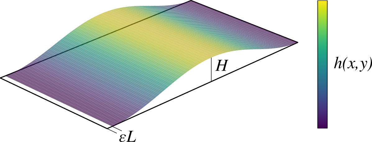
Figure 1: Parametrization of the elastic sheet for the analysis of buckling. The black lines represent the flat configuration.

We examine a defect-free sheet under an uniaxial compressive load. In this context, an approximate analytic expression may be derived, which provides relevant insights into the elastic behavior encoded in the sAPFC model accounting for the out-of-plane displacement.

As illustrated in Fig. 1, we consider a uniform sheet of length $L$ in the direction of compression, with an initial strain $\varepsilon<0$, which buckles with a maximum height $H\geq 0$. In the APFC model, the displacement field $\mathbf{u}$ is encoded in the phase of the complex amplitudes (Salvalaglio and Elder, 2022):

$$\eta_{n}=|\eta_{n}|e^{-\mathbbm{i}\mathbf{k}_{n}\cdot\mathbf{u}}.$$ (29)

Introducing this expression in the energy (17), the stationary solution is given by the conditions:

$$\frac{\delta\mathcal{F}_{\eta}}{\delta|\eta_{n}|}=0,\quad\frac{\delta\mathcal{F}_{\eta}}{\delta h}=0,\quad\frac{\delta\mathcal{F}_{\eta}}{\delta\mathbf{u}}=\mathbf{0}.$$ (30)

These equations yield a highly nonlinear system of coupled equations that cannot be easily solved in its current form. We proceed further via Taylor expansions near the critical buckling point, corresponding to where the sheet is maximally compressed while remaining flat. Importantly, we take advantage of two different approximations: a geometric one (small surface height gradients $HQ\ll 1$) and a physical one (small deformations $|\varepsilon|\ll 1$), where $Q=2\pi/L$ denotes the wave number of the buckling profile. At the critical buckling point, the height profile and displacement field take the form:

$$h_{0}(y)=0,\quad\mathbf{u}_{0}(x,y)=u_{0}(y)\mathbf{e}_{y}=\varepsilon_{c}y\,\mathbf{e}_{y}.$$ (31)

In the limit of small surface height gradients, i.e., $g\equiv HQ\ll 1$, they can be expanded such that:

$$h(y) =h_{0}(y)+gh_{1}(y)+g^{2}h_{2}(y)+\mathcal{O}(g^{3}),$$ (32)

$$u(y) =u_{0}(y)+gu_{1}(y)+g^{2}u_{2}(y)+\mathcal{O}(g^{3}).$$ (33)

At lowest order, the condition $\delta\mathcal{F}_{\eta}/\delta h=0$ yields:

$$h_{1}(y)=H\cos\left((1-\varepsilon_{c})\sqrt{\frac{A}{2\kappa}|\varepsilon_{c}|(2-\varepsilon_{c})(|\eta_{1}|^{2}+8|\eta_{2}|^{2})}\,y\right).$$ (34)

The periodicity of the system then imposes

$$(1-\varepsilon_{c})\sqrt{\frac{A}{2\kappa}|\varepsilon_{c}|(2-\varepsilon_{c})(|\eta_{1}|^{2}+8|\eta_{2}|^{2})}=Q.$$ (35)

By denoting

$$\varepsilon_{c,0}=-\frac{\kappa Q^{2}}{A(|\eta_{1}|^{2}+8|\eta_{2}|^{2}|)},$$ (36)

we then have the relation

$$\varepsilon_{c}=1-\sqrt{\frac{1+\sqrt{1-8\varepsilon_{c,0}}}{2}}.$$ (37)

Using the condition $\delta\mathcal{F}/\delta\eta_{n}=0$, one may show that

$$|\eta_{n}|=\phi+\varepsilon_{c}^{2}\phi_{n}+\mathcal{O}(\varepsilon_{c})^{3}.$$ (38)

By inserting (38) into (37) eventually leads to:

$$\varepsilon_{c}=\varepsilon_{0}+\frac{5}{2}\varepsilon_{0}^{2}+\mathcal{O}(\varepsilon_{0}^{3}),$$ (39)

with $\varepsilon_{0}=-\kappa Q^{2}/(9A\phi^{2})$. Similarly, we compute:

$$h_{2}(y)=u_{1}(y)=0,\quad u_{2}(y)=\varepsilon_{2}y+U_{2}\sin(2Qy),$$ (40)

with

$$\left\{\begin{aligned} \varepsilon_{2}&=\frac{-3(1-\varepsilon_{c})^{3}}{8-16\varepsilon_{c}(2-\varepsilon_{c})}+QU_{2}=-\frac{1}{4}-\frac{15\varepsilon_{0}+4Q^{2}}{24}+\mathcal{O}(\varepsilon_{0}^{2}),\\ QU_{2}&=\frac{(1-\varepsilon_{c})(1-2\varepsilon_{c}(2-\varepsilon_{c}))}{8(1-\frac{3}{2}\varepsilon_{c}(2-\varepsilon_{c})+\frac{4}{3}Q^{2})}=\frac{1}{8}-\frac{3\varepsilon_{0}+2Q^{2}}{12}+\mathcal{O}(\varepsilon_{0}^{2}).\end{aligned}\right.$$ (41)

From the boundary condition

$$u(L)=\varepsilon_{c}L+(HQ)^{2}\varepsilon_{2}L=\varepsilon L,$$ (42)

we conclude, assuming $\varepsilon\sim\varepsilon_{0}$ and at leading order in $Q\ll 1$:

$$(HQ)^{2}=\frac{\varepsilon-\varepsilon_{c}}{\varepsilon_{2}}=-4(\varepsilon-\varepsilon_{0})+10\varepsilon_{0}\varepsilon+\mathcal{O}(\varepsilon_{0}^{3}).$$ (43)

The derivation for higher-order approximations follows the same procedure, and we only report the final expression for brevity. Taking into account the next relevant orders in surface height gradients $\mathcal{O}(g^{5})$ and critical strain $\mathcal{O}(\varepsilon_{0}^{4})$, we obtain:

$$\begin{split}(HQ)^{2}=&-4(\varepsilon-\varepsilon_{0})+\frac{7}{6}\left(\varepsilon^{2}+\varepsilon_{0}^{2}+\frac{46}{7}\varepsilon_{0}\varepsilon\right)\\ &-\frac{49}{72}\varepsilon^{3}+\frac{19}{2}\varepsilon^{2}\varepsilon_{0}+\frac{245}{24}\varepsilon_{0}^{2}\varepsilon-\frac{73}{36}\varepsilon_{0}^{3}\left(1+\frac{32}{73}\frac{\phi_{1}+8\phi_{2}}{\phi}\right)+\mathcal{O}(\varepsilon_{0}^{4}).\end{split}$$ (44)

Figure 2: Buckling of a sheet in the elastic regime. (a) sAPFC simulation results (black circles) in terms of $H^{2}$ (see parametrization in Fig. 1) against bending stiffness $\kappa$ for $\varepsilon=-0.025$, compared to different analytical approximations (lines): gray $\mathcal{O}(\varepsilon_{0}^{2},g^{3})$, orange $\mathcal{O}(\varepsilon_{0}^{3},g^{3})$, blue $\mathcal{O}(\varepsilon_{0}^{3},g^{5})$, and red $\mathcal{O}(\varepsilon_{0}^{4},g^{5})$. (b) and (c) show details of the plot in (a) at low and large bending stiffness, respectively.

To test this prediction, we simulate buckling at different bending stiffnesses with the sAPFC  model. For this test, we may also refer to the results for the PFC model encoding out-of-plane deformations reported in Elder et al. (2021) for comparison. Importantly, we remark that no simplification enforcing the limit of small height gradients is considered in the expression of the differential operator and the bending energy term for the sAPFC  model.

Figure 3: Assessment of the buckling behavior encoded in the sPFC  model. (a) sPFC  simulation results (black circles) in terms of $H^{2}$ (see parametrization in Fig. 1) against bending stiffness $\kappa$ for $\varepsilon=-0.0219$ as from Elder et al. (2021), compared with the highest-order analytical expression with the approximated (red) and non-approximated (blue) versions of the energy. (b) and (c) show details of the plot in (a) at low and large bending stiffness, respectively.

A suitable compressive (tensile) strain to be used in the (s)APFC model must retain an integer number of lattice sites in the domain, meaning an integer number of atomic rows must be introduced (removed). This ensures periodicity at the boundaries and compatibility with the Fourier pseudo-spectral method chosen to solve the equations numerically. For the simulations, we consider a system with $N=40$ the number of atoms in the compression direction, $\varepsilon=-1/40=-0.025$, and use the following set of parameters: $(A,B,C,D)=(1,-0.15,1/2/\sqrt{0.98/3},1)$ (Hirvonen et al., 2017), which leads to a honeycomb lattice structure.

We present in Fig. 2 sAPFC simulation results of bucking in terms of $H^{2}$ (with $H$ the maximum height, see Fig. 1) by varying the bending stiffness. Moreover, we compare them to the various analytical approximations reported above. While the lowest order approximation captures the overall correct behavior, there is a clear difference in both regions of small and large bending stiffness $\kappa$. By considering a higher order of surface height gradient, excellent agreement is now obtained in the region of low bending stiffness/large buckling height. Similarly, higher orders of the critical strain lead to excellent agreement in the region of large bending stiffness/small buckling height. This underlines the different roles played by the two approximations: the physical one ($\varepsilon_{0}\ll 1$) with a strong effect in the region of large bending stiffness, and the geometric one ($g\ll 1$) with a substantial impact in the region of large buckling height. As illustrated in the insets of Fig. 2, in the region of large buckling height, the $\mathcal{O}(g^{5})$-approximations behave identically despite different $\varepsilon_{0}$-orders, and similarly in the region of large bending stiffness, the $\mathcal{O}(\varepsilon_{0}^{3})$-approximations behave identically despite different $g$-orders.

We also compare in Fig. 3 the sPFC results to the highest-order analytical prediction. Unsurprisingly, as the differential operator and the bending energy are approximated by their leading order in terms of the surface height gradients, a clear difference is visible in the region of large buckling height. By modifying the analytical derivations to account for these simplifications, the predicted buckling height relation reads:

$$\begin{split}(HQ)^{2}=&-4(\varepsilon-\varepsilon_{0})-\frac{19}{2}\left(\varepsilon^{2}+\varepsilon_{0}^{2}-\frac{58}{19}\varepsilon_{0}\varepsilon\right)\\ &-\frac{361}{8}\varepsilon^{3}+\frac{1177}{6}\varepsilon^{2}\varepsilon_{0}-\frac{4235}{24}\varepsilon_{0}^{2}\varepsilon+\frac{509}{12}\varepsilon_{0}^{3}\left(1-\frac{32}{152}\frac{\phi_{1}+8\phi_{2}}{\phi}\right)+\mathcal{O}(\varepsilon_{0}^{4}),\end{split}$$ (45)

and we recover an excellent agreement. Interestingly, looking back at Eq. (43) as a function of $\kappa$:

$$(HQ)^{2}=-4\varepsilon-\frac{4\kappa Q^{2}}{9A\phi^{2}}\left(1+\frac{5}{2}\varepsilon\right)\simeq-4\varepsilon-\frac{4\kappa Q^{2}}{9A\left[\left(1-\frac{5}{4}\varepsilon\right)\phi\right]^{2}},$$ (46)

we observe that the higher-order $\mathcal{O}(\varepsilon_{0}^{3},g^{3})$ expression matches the $\mathcal{O}(\varepsilon_{0}^{2},g^{3})$ expression if the amplitude is corrected by a factor $1-(5/4)\varepsilon$ (see denominator of the final expression in Eq. (46)). For $\varepsilon=-0.0219$, this quantity $1-(5/4)\varepsilon=1.027$ matches the correcting factor of $1.031$ proposed in Elder et al. (2021) to have the lower-order approximation fit the simulation results.

Regarding the buckling behavior, we may conclude that: i) the sAPFC  model reproduces almost perfectly the sPFC  behavior, and ii) it encodes a description of elasticity beyond infinitesimal deformations. Moreover, we reported here a rigorous analysis shedding new light on the correction proposed in Elder et al. (2021), which actually serves to compensate for the low-order expansion in the critical strain. Additionally, we remark on two important aspects of considering the sAPFC  model instead of the sPFC  model. Without any defect to resolve, the sAPFC  has a significant computational advantage as a very coarse mesh, which only needs to resolve the slowly varying height profile, can be used. For instance, the sAPFC  simulations are conducted with $\delta x=\delta y\simeq 31.4$ (as well as $15.7$ and $7.9$ to verify convergence), whereas the sPFC  simulations required $\delta x=\delta y\simeq 0.48$ to resolve the microscopic density field $\psi$ correctly. Moreover, amplitudes can be directly used to compute the elastic field (Salvalaglio et al., 2019, 2020) without using additional filtering and numerical coarse-graining procedures (Skogvoll et al., 2021, Elder et al., 2021), as will also be exploited in the following.

4 Defect arrangements on a fixed surface profile

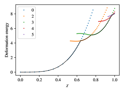
Figure 4: Deformation energy ($\mathcal{F}_{\eta,\mathcal{S}}-\mathcal{F}_{0}$) as a function of the aspect ratio ($\chi$) for the sAPFC  model. The dotted curves correspond to simulations with a given number of dislocations (see legend). Energy parameters (see Eq. (17)): $A=2$, $B=0.02$, $C=-1/2$, and $D=1/3$.

To analyze the interplay between out-of-plane deformation and lattice distortion, we now study the relevant case of defect stability and arrangement on a distorted crystalline sheet. We consider first the simplifying assumption of a fixed height profile. Indeed, out-of-plane deformations stretch the lattice, creating strains that may be relieved by an appropriate distribution of defects, depending on the competition between the elastic strain energy and the defect energy. To assess the influence of curvature on defect configurations, we choose a substrate in the shape of a Gaussian bump with standard width $\rho$ such that

$$h(x,y)=\chi\rho e^{-\frac{x^{2}+y^{2}}{2\rho^{2}}},$$ (47)

with varying aspect ratio $\chi$. As a demonstration of the scale-bridging capabilities of the sAPFC  model, simulation results are compared with atomistic-scale Monte Carlo (MC) computations reported in (Hexemer et al., 2007) as well as the continuum-scale theory derived in (Vitelli, 2006). Additionally, sPFC  simulations of the same system are presented, further showcasing the effectiveness of the coarse-graining employed in the sAPFC  model.

Figure 5: Configurations of defects forming in a crystalline sheet upon its deformation with a Gaussian profile as in Eq. (47) obtained by the sAPFC  model. The transition from circular defect arrangements (for a number of defects less than or equal to four) to asymmetric arrangements (for more than four defects) is showcased. (a) 2-defect configuration in a 3D perspective view; (b) 3-defect configuration. Clockwise from the top: reconstructed density from the amplitudes (38), $\Phi=\sum_{n=1}^{3}|\eta_{n}|^{2}$ (blue-to-red color scale), Delaunay triangulation of density maxima in top view; (c)-(f) Delaunay triangulation of density maxima in top view for 4-, 5-, 6-, and 7-defect configurations, respectively. Aspect ratios ($\chi$) of the Gaussian deformation profile for the different panels are (a) 0.7, (b) 0.8, (c) 1.0, (d) 1.0, (e) 1.0, (f) 1.6. In all panels, dislocations are represented by the Voronoi cells of fivefold (red) and sevenfold (blue) disclinations. Same energy parameters as in Fig. 4.

The deformation energy and number of defects as a function of the aspect ratio are plotted for the sAPFC  model in Fig. 4. The globally minimizing configuration is indicated as the continuous line. We also represent local minimizers corresponding to metastable states (reachable by specifying different initial conditions) to illustrate the competition between elastic and defect energy. The existence of a critical aspect ratio—below which the lattice is frustrated but defect-free and above which the nucleation of defects becomes energetically favorable—is thus made evident. Further, at a given number of defects, the surface energy seems to follow a U-shaped curve that scales as a power law near its minimum. The energy and aspect ratio associated with this minimum point increase with the number of defects in the configuration. This explains the particular shape of the deformation energy-aspect ratio curve as a smoothly broken power law (i.e., a piecewise function given by a sequence of conjoined power laws). For a defect-free surface, the energy can be closely fit to a $\chi^{4}$-dependency, matching the analytical prediction with great accuracy (Vitelli, 2006), despite our setting not strictly meeting the theoretical requirements. Indeed, the analytical expression was derived in the continuum limit $\rho\ll b$ ($b$ the lattice parameter) and neglecting boundary effects $L\gg\rho$ ($L$ the domain size), while in our simulations, $\rho/b\simeq 4.1$ and $L/\rho\simeq 6.3$. Nevertheless, the authors have also shown with MC simulations that the analytical results correctly describe the problem beyond their strict validity domain: a conclusion our computations corroborate.

We additionally report the different minimizing defect arrangements in Fig. 5. We note that for four dislocations and less, the minimizing defect configuration consists of a symmetric circular arrangement. This symmetry is lost for five dislocations and more, as the repelling force between dislocations increases, in complete agreement with the MC simulations (Hexemer et al., 2007). For very large aspect ratios ($>1.5$), we also recover the same branching behavior of dislocations distributing themselves along scars, similarly to what is observed on spherical crystals (Bausch et al., 2003, Backofen et al., 2011), thus evidencing the applicability of the proposed model beyond small deformations.

In short, an excellent qualitative agreement is obtained between the sAPFC  model and MC simulations (Hexemer et al., 2007). The extension of the sAPFC  model to surfaces conserves the qualities of its flat space counterpart: by solving for slowly varying fields while retaining the microscopic details of the underlying lattice structure, it can correctly capture details such as the defect arrangements around the bump, while also recovering the energy scaling predicted by the continuum-level theory (Vitelli, 2006). Given that an arbitrary set of parameters was used in the MC simulations (Hexemer et al., 2007), not informed by any real material elastic properties, a quantitative agreement is not possible.

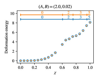
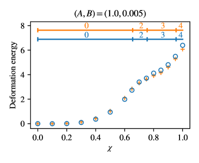
Figure 6: Deformation energy ($\mathcal{F}_{\eta,\mathcal{S}}-\mathcal{F}_{0}$) for the system in Fig. 5 as a function of aspect ratio for both the sPFC  model (blue circles) and sAPFC  model (orange crosses). The two plots show the results obtained for $(C,D)=(-1/2,1/3)$ as in Fig. 4, with two choices of the energy parameters $A$ and $B$ reported in the panels (see definition of the energy in Eq. (17)). The number of defects in the energy-minimizing configuration for different $\chi$, coinciding for the two considered models, is also reported; see the segmented lines on the top part of the plots (colors correspond to the simulation results).

Since the sAPFC  model is obtained as a coarse-grained sPFC  model, we now present comparative results of the two models in Fig. 6 to inspect the validity of the coarse-graining approximation more specifically. The agreement between these models is almost perfect for both the energy and the number of dislocations. This confirms the validity of the coarse-graining underlying the devised mesoscale framework. In particular, using the flat scalar product approximation on curved substrates does not introduce spurious effects in the presence of both lattice deformation and defect nucleation, i.e., the phenomena we aim to describe with our approach. We note that this holds in a setting where the maximum height gradients reach $0.61$ for $\chi=1$, which is far beyond the small deformation limit. Nevertheless, for $\chi>0.5$, the surface energy is observed to be slightly higher ($1\%$ at most) in the sPFC  simulations compared to the sAPFC  results, which might be ascribed to that approximation. We find that the number of defects and the energy depends on the energy parameters $A$, namely controlling elastic constants, and $B$ corresponding to the quenching depth (Skogvoll et al., 2023) (the latter being the parameter controlling the order-disorder/solid-liquid phase transition for $B\lessgtr B_{c}$, with $B_{c}$ the critical point). We find that the agreement illustrated in Fig. 6 holds for relatively large values of $A$ (typically $A\geq 2$). At lower values of $A$, the cohesion between atoms becomes very weak, mimicking a colloidal behavior, which is naturally not reproducible by APFC models, as it enforces a lattice structure through Eq. (16). Nevertheless, since our focus is on modeling crystalline structures, the comparison at these low $A$ values is not meaningful.

When sufficiently close to the solid-liquid transition ($B\sim B_{c}$), we observe that partial melting at the top of the bump is the most energetically favorable state with the sPFC  model. The sAPFC  with the approximation of constant average density $\overline{\psi}$ (see discussion of Eq. (25)) still predicts a fully crystallized phase. Indeed, the same melting point is obtained by solving the full system of equations (23)–(25). We note, however, that the variation of $\overline{\psi}$ at defects is more pronounced in the APFC models with non-constant $\overline{\psi}$ than in the PFC models (which we also verified for the flat case), affecting their energy and thus the comparison shown in Fig. 6. This effect can be ascribed to additional approximations entering the derivation of the flat-space counterpart of Eq. (25), as widely discussed in Yeon et al. (2010). Aiming here at describing thin sheets in the crystalline state, we then propose to use the sAPFC  model with constant $\overline{\psi}$ providing an accurate coarse-graining as seen in Fig. 6. Further explicit comparisons and discussions are reported in C.

We have also conducted a study on a double sine-wave surface, i.e.,

$$h(x,y)=\chi L_{x}/(2\pi)\sin(2\pi/L_{x}x)\sin(2\pi/L_{y}y).$$ (48)

featuring a more complex distribution of curvatures and expected behaviors. For low enough aspect ratios, we recover defect arrangements consistent with microscopic models again (Hexemer et al., 2007), see Fig. 7. At aspect ratios larger than 0.8, microscopic models predict the nucleation of disclinations to reach the global minimum energy state. We remark that these defects cannot be modeled in the current sAPFC framework as they break the rotational symmetry of the crystal, while they may be accessible with the sPFC  model (Backofen et al., 2011). We may then conclude that the sAPFC  model qualitatively captures the essential features of defect nucleation and arrangements on a curved substrate for finite aspect ratios, beyond the classical small (ideally infinitesimal) deformation limit. Further, quantitative agreement with the sPFC  model is also excellent in the parameter space of interest, indicating minimal loss of information due to spatial coarse-graining.

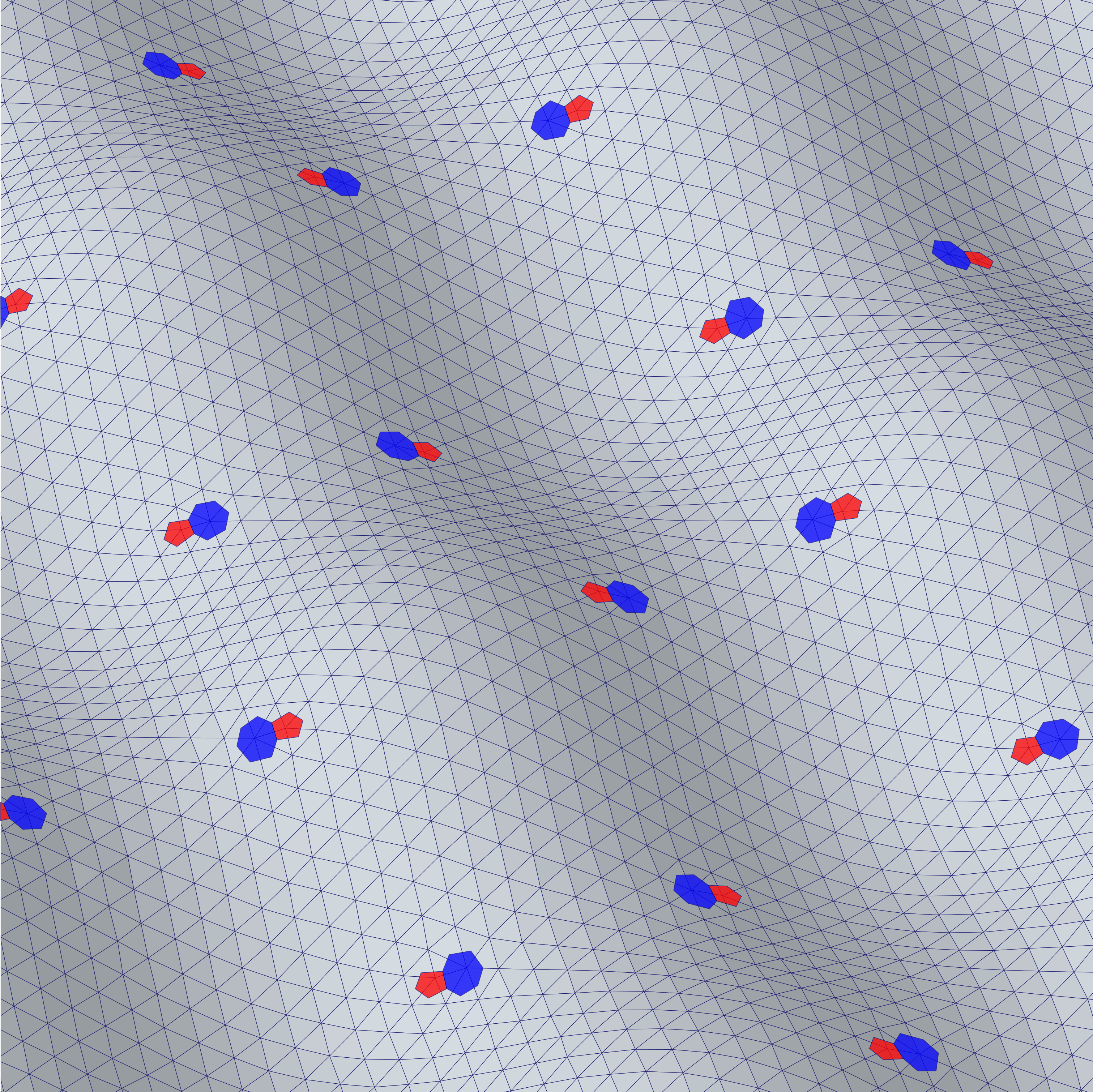
Figure 7: Representative sAPFC simulation of defect arrangements on a deformed sheet featuring a double sine-wave height profile. Delaunay triangulation of density maxima and dislocations are illustrated as in Fig. 5. Same energy parameters as in Fig. 4.

5 Surface profile at a dislocation

After studying how crystalline sheets adapt to a fixed height profile through defect nucleation, we now look at the out-of-plane deformation induced by dislocations. Indeed, generally speaking, but particularly in 2D materials, dislocations have been shown to play a determinant role in elucidating material properties and grain boundary structures (Fan et al., 2017, Azizi et al., 2017, Hirvonen et al., 2017). In graphene, dislocations commonly give rise to a Stone-Wales defect, consisting of a $5|7$ pair of rings rather than the six-ring equilibrium honeycomb structure, as illustrated in Fig. 8(a). These defects generate long-range elastic fields, which can be reduced by out-of-plane displacement. To study this phenomenon, we analyze the relaxation of a sheet hosting a dislocation pair—or more accurately in our case, of two identical dislocation pairs, due to the periodic boundary constraint.

While on a flat-constrained sheet, this defect configuration is stable due to the periodicity of the system, it is no longer the case when the fully coupled model is considered, and the out-of-plane displacement breaks the symmetry: the dislocations are observed to migrate away from the bulge they create, and towards each other, until annihilation. In the sPFC  model, this behavior should be expected close to melting point only as it involves a motion by climbing that is prevented by pinning at relatively low quenching depths (Skaugen et al., 2018b, Elder et al., 2021). To mimic fixed dislocations, i.e., to obtain a pseudo-stationary surface height profile, we reset the dislocation cores at their initial positions if they migrate by shifting the crystal and interpolating the missing data. As this interpolation occurs far away from the dislocations, its influence on the resulting height is negligible, as we verified by checking the convergence of the numerical results. The study of the complete dislocation dynamics is presented in the following section.

Figure 8: Out-of-plane deformation at a dislocation by the sAPFC  model. A small portion (13$a_{x}$ x 13$a_{x}$) centered around a dislocation of a domain of total size (141$a_{x}$ x 40$a_{y}$) is shown for $\kappa=\kappa_{g}\simeq 0.21$ Dai et al. (2016), where $a_{x}=4\pi/\sqrt{3}$ and $a_{y}=4\pi$ are the lattice parameters in the $x$ and $y$ directions, respectively. (a) Reconstructed density on a perspective view of the deformed crystalline sheet, (b) surface height profile $h$, (c) $\partial_{x}h$ , and (d) $\partial_{y}h$. The colormap was chosen to match the one in Elder et al. (2021). The maxima of the reconstructed density are shown as black dots in panels (b)–(d). Same energy parameters as in Sect. 3: $A=1,B=-0.15,C=0.87$, and $D=1$.

A portion of the system near one of the dislocation cores is presented in Fig. 8. The resulting height profile and gradients are in very good agreement with the sPFC predictions (Elder et al., 2021): the surface is essentially flat above the dislocation core but shows significant variations near and below it. Note that while the sAPFC model solves for the amplitudes, it is straightforward to reconstruct the corresponding atomic density from them via Eq. (16), and recover the typical 5|7 Stone-Wales defect observed in graphene.

To compare the classical elasticity theory predictions in flat space with the numerically simulated results with the s(A)PFC models, the stress fields have been calculated from the amplitudes extending the approaches proposed in Skaugen et al. (2018b), Salvalaglio et al. (2019, 2020) to deformable surfaces, which yields:

$$\begin{split}\frac{\sigma_{\alpha\beta}}{A}=&-v_{\alpha}\sum_{n=-N}^{N}\left[\mathcal{G}_{n}^{\mathcal{S}}\eta_{n}\right]\left[(\partial_{\beta}-\mathbbm{i}k_{n,\beta})\eta_{n}^{*}\right]+\sum_{\gamma=1}^{2}\left\{w_{\alpha\gamma}\sum_{n=-N}^{N}\left[(\partial_{\gamma}+\mathbbm{i}k_{n,\gamma})\mathcal{G}_{n}^{\mathcal{S}}\eta_{n}\right]\left[(\partial_{\beta}-\mathbbm{i}k_{n,\beta})\eta_{n}^{*}\right]\right.\\ &-\left[\mathcal{G}_{n}^{\mathcal{S}}\eta_{n}\right]\left[(\partial_{\beta}-\mathbbm{i}k_{n,\beta})(\partial_{\gamma}-\mathbbm{i}k_{n,\gamma})\eta_{n}^{*}\right]+(\partial_{\gamma}w_{\alpha\gamma})\left[\mathcal{G}_{n}^{\mathcal{S}}\eta_{n}\right]\left[(\partial_{\beta}-\mathbbm{i}k_{n,\beta})\eta_{n}^{*}\right]\left.\vphantom{\sum_{n}^{N}}\right\}\end{split}$$ (49)

where

$$v_{\alpha} =\frac{\partial(\nabla^{2}_{\mathcal{S}}\psi)}{\partial(\partial_{\alpha}\psi)}=\frac{-\mathcal{H}}{\sqrt{|\boldsymbol{g}|}}\,\partial_{\alpha}h,$$ (50)

$$w_{\alpha\gamma} =\frac{\partial(\nabla^{2}_{\mathcal{S}}\psi)}{\partial(\partial_{\alpha\gamma}\psi)}=\delta_{\alpha\gamma}-\frac{(\partial_{\alpha}h)(\partial_{\gamma}h)}{|\boldsymbol{g}|}.$$ (51)

In the flat case, $\boldsymbol{v}=\boldsymbol{0}$, $\boldsymbol{w}=\mathbf{Id}$, and we recover the flat surface formula. Note that in (s)PFC models, the stress field must be reconstructed from the density. When the density field is used as is, the obtained stress field is only defined up to a divergence-free gauge (Skogvoll et al., 2021) and also requires additional filtering to remove atomistic-length scale fluctuations (Elder et al., 2021), with an arbitrarily set filtering kernel. Another common approach relies instead on extracting the complex amplitudes from the density field so the stress field can then be computed with (49). While this eliminates the divergence-free gauge, an arbitrary length scale is still required for the demodulation. By contrast, the (s)APFC model solves for the amplitudes directly and thus allows for straightforward access to the stress field.

Figure 9: Stress field at a dislocation computed by equation (49) from the results of sAPFC  simulations with: $\kappa=\kappa_{g}\simeq 0.21$ (blue dotted line), $\kappa=4\kappa_{g}\simeq 0.84$ (red dash-dotted line), rigid sheet $\kappa\rightarrow\infty$ (black solid line). The prediction of continuum mechanics in a flat domain (Anderson et al., 2017) is also shown (black dashed line). Same energy parameters as in Fig. 8.

The calculated stress fields are detailed in Fig. 9. We observe a regularization of the stress field at the dislocation core, as is typical for (A)PFC model (Salvalaglio et al., 2019, 2020, Skogvoll et al., 2023). Away from the core ($\sim$ 3 atomic spacings), there is excellent agreement between the linear elasticity theory (Anderson et al., 2017), the sPFC  model, and the sAPFC  model. More importantly, we note that out-of-plane displacements lead to the localization of the compressive stress closer to the dislocation core by buckling, with softer surfaces (smaller $\kappa$) allowing for greater localization. While the same qualitative behavior is observed in the sPFC results of Elder et al. (2021), there exists a clear difference in the stress reduction at the core, particularly noticeable in Fig. 9(a). For instance, our results indicate a negligible reduction of $\sigma_{xx}$ at the dislocation core when using the sAPFC  model, while the sPFC  model predicts it to be halved. This might be a consequence of the approximation used in the sPFC  model that neglects high-order nonlinear contributions as well as the smoothing kernel used to reconstruct the stress field, which leads to some reduction of the stress at the dislocation core, pointed out by the authors.

We have thus shown that in the fully coupled setting, the coarse-grained picture offered by the sAPFC still captures all the features from the PFC results. Importantly, it gives direct access to the stress field and enables the inspection of large systems.

6 Dislocation interaction

In order to analyze how the out-of-plane deformation influences dislocation interaction, we compare the velocities of a pair of dislocations in different representative configurations of the Burgers vectors and initial surface profiles. The amplitude fields are initialized to represent a pair of dislocations with a distance of 28 atomic units in a square domain of linear dimension of 171 atomic units via the corresponding displacement field and superimposing the fields from the periodic images (Salvalaglio et al., 2020).

We look at symmetric configurations where the dislocations are aligned along the y direction. In particular, two configurations are considered: (I) a dislocation at the top (bottom) having Burgers vector parallel (anti-parallel) to the x direction and (II) dislocations as in I but with opposite Burgers vectors. These defects are expected to annihilate by climbing. Regarding the surface profile, an initial guess consisting of Gaussian bumps centered at each dislocation is chosen. Note that we cannot start from a perfectly flat surface as it represents a stationary condition for the height profile. We consider three cases: i) flat space, ii) upward buckling at each dislocation (denoted by UU), and iii) upward buckling at one dislocation and downward buckling at the other (denoted by UD).

By choosing a very high ratio between the height and amplitude mobilities (typically $M_{h}/M_{\eta}=1\times 10^{5}$), we are then able to relax the height and amplitudes to a lower energy configuration while almost completely freezing the movement of the dislocations. Because the system is inherently out of equilibrium, we can not reach a true stationary profile. Instead, this procedure allows us to get a pseudo-stationary height profile, which we use to initialize a simulation where the dislocations can move to study their velocities (with $M_{h}/M_{\eta}=2000$).

Figure 10: Effects of the out-of-plane deformation on dislocation annihilation (by climbing). (a)-(d) Four representative configurations featuring different combinations of opposite Burgers vector and upward/downward dislocation-induced sheet deformation. Each panel shows $\sigma_{yy}$ (left) and the height profile (right). (e) Dislocation distance as a function of time for the various representative configurations (lines are only guides for the eye). Energy parameters: $A=2,B=0.02,C=-1/2$, and $D=1/3$.

The results are shown in Fig. 10. In the flat setting, the dislocations merge towards the center in 28500 and 28000 timesteps in the I and II configurations, respectively. Such a slight difference emerges from the asymmetry in the magnitude of compressive/tensile lattice deformation due to nonlinear effects (Hüter et al., 2016). Different signs of the stress lobes within the dislocations in the two configurations are obtained, thus driving the motion of the dislocation consistent with the classical Peach-Köhler equation (Skogvoll et al., 2022a) with slightly different velocities. Out-of-plane deformation contributes to dislocation motion, as mentioned in the previous section. A bulge forms at the region close to the dislocation with negative hydrostatic stress. The dislocation then moves towards the opposite side while dragging the deformed surface. In other, perhaps more visual, words, the dislocations “surf” on the bulge they each create. As a result, when considering the dipoles in a deformable sheet, the dislocations merge faster than in the flat when the bulges form outside the region between the dislocations, corresponding to the I configuration. On the other hand, when the bulges are between the dislocations, as in the II configuration, the movement of the dislocations is considerably slowed down, even moving away from the center initially, as the motion induced by the out-of-plane deformation is opposite to the one dictated by the elastic driving force.

Focusing on the I setting, we take a closer look at the dynamics of the dislocation merging. At initial times, when the dislocations are far enough from each other, the interactions between their respective bulges are minimal, and the distance evolution in time is identical in the UU and UD settings. The merging velocity also appears to be greater than in the flat case. Still, we refrain from specific quantitative comments as this result depends on the mobility ratio and the pseudo-stationary surface profile used for initialization. Then, as the dislocations get closer and the bulges they create interact, we see the merging velocity in the UD case decrease relative to its UU counterpart. In short, while an upward bulge drives the dislocation identically to a downward one, as expected from surface symmetry, the interaction of two identical bulges is significantly different from that of opposite bulges. Therefore, besides an additional driving force on a single dislocation, the out-of-plane deformation also mediates an effect on dislocation-dislocation interaction. Similar considerations can be devised by looking at the II configurations. Moreover, notice that the bending stiffness of the deformable sheet is expected to affect this behavior as it directly controls the magnitude of out-of-plane deformation. This is illustrated by considering the II-UU case for two different values of $\kappa$; c.f. II-UU and II-UU (2$\kappa$). Larger values of this parameter lead to less significant out-of-plane deformation and, in turn, a reduced contribution of the bulge-induced motion with the flat surface limit consistently reached for $\kappa\rightarrow\infty$.

We have seen that interactions between dislocations on a deformable sheet are significantly more complex than in a flat (rigid) domain. In the following, we additionally show that dislocation interaction in systems hosting many dislocations may also be mediated by surface wrinkling and lead to highly non-trivial behaviors in terms of surface deformation at and close to defects.

7 Thin sheets hosting many dislocations: an example

We present the results of a relatively large-scale simulation reproducing a deformable sheet hosting many dislocations. In a square domain of linear dimension 340 a.u., we first introduce (arbitrarily) 256 dislocations at random positions via the appropriate displacement field from linear elastic theory. Without loss of generality for the targeted evidence, and to facilitate the discussion, we consider Burgers vectors along the $x$-axis only. Then, because this initial displacement field from elastic theory is singular, we let the system relax in the flat for a short time to allow the amplitudes to adjust. In that time, dislocation annihilations occur, resulting in a final system containing 87 dislocations. This relaxed configuration is then taken as the initial condition for the fully coupled simulation with out-of-plane displacements—where an upward out-of-plane bump has been introduced at each defect—and we let the system evolve. As dislocations move, driven by both dislocation-induced elastic field (as in the flat) and out-of-plane deformation, we obtain an overview of all aspects described in previous sections as well as new phenomena, deriving from the complex interactions between dislocations (see Fig. 11). For instance, the various dislocation bulges may interact to create a wrinkled surface. Likewise, while the surface profile at all dislocations was initialized as an upward bulge, we notice that it may flip to a downward bulge due to interaction with another dislocation, which is consistent with the fact that both configurations are indistinguishable from an energy standpoint. Also, in the presence of non-trivial dynamics, a combination of the phenomenology presented in Fig. 10 may occur.

A final comment concerns the height profile after the annihilation of a dislocation pair. Indeed, due to the relatively low ratio between the mobilities for the height profile and the amplitudes—arbitrarily chosen to observe dislocations moving and dragging their bulges while keeping a reasonable computation time—, the out-of-plane deformation slowly flattens out with time after dislocation annihilation. The corresponding timescale may be controlled with the mobility ratio and varied to explore different regimes. Moreover, it must be pointed out that we consider here a purely diffusive dynamics considered for the amplitudes that cannot capture fast elastic response. Formulations accounting for this regime have been proposed for the classical APFC model (Heinonen et al., 2016, Salvalaglio et al., 2020). However, the extension of these approaches to deformable thin sheets in the formulation considered here is non-trivial. It will be the object of future work together with quantitative inspections of dislocation interactions.

Figure 11: Buckling of a crystalline sheet (side length 340 a.u.) initially hosting 87 dislocations, at times (a) 0, (b) 5000, and (c) 10000. The contour plot shows the height profile. The dislocations are indicated by the black dots. A few noteworthy features: (⃝) remnant bulge after dislocation pair annihilation, ($>$) wrinkling, and ($\rightarrow$) upward bulge flipping to a downward bulge. (d)-(e) 3D view of panel (b) and the inset therein. Same energy parameters as in Fig. 10.

8 Conclusion

We provided a framework for gradient-flow equations on deformable surfaces—based on a height formulation where normal surface deformation is considered—that allowed us to extend the description of crystal lattices conveyed by PFC and APFC models to non-flat surfaces. We focused, in particular, on the latter in several relevant settings. Excellent agreement between sPFC  and sAPFC  models was found in both elastic and plastic regimes, demonstrating the ability of the sAPFC  model to accurately describe dislocations and interfaces on deformable surfaces while solving for slowly varying fields. Importantly, this can enable large-scale simulations using mesh-adaptivity techniques (Athreya et al., 2006, Berčič and Kugler, 2018, Praetorius et al., 2019).

For defect-free surfaces, the sAPFC  formulation encodes an advanced and efficient description of elasticity accounting for out-of-plane deformation. In this context, the model could prove extremely useful in studying crystalline sheets deformed elastically, e.g., for vibration dynamics and thermal buckling in graphene, upon considering proper extensions such as including thermal noise (Granato et al., 2023).

For defects on a fixed surface, we have shown that the sAPFC  model is in qualitative agreement with atomistic models, as it captures the essential features of defect stability and arrangements on a Gaussian bump. Additionally, excellent agreement with the PFC model again substantiates the effectiveness of the sAPFC  model in retaining microscopic features while solving for spatially coarse-grained quantities.

It is worth mentioning that in microscopic theories, Fourier-mode analysis of microscopic density fields is generally employed to study slowly varying fields, i.e., with quantities analogous to the amplitude functions. The stress field is a prototypical example of a slowly varying field compared to atomistic length scales. Nevertheless, it determines behaviors such as dislocation interaction and dynamics, which are inspected by micro- and mesoscopic models. In PFC models, either complex amplitudes are adopted to derive stress and strain fields, or the microscopic stress is evaluated and coarse-grained based on smoothing routines. In both approaches, the deformation of defects depends on regularization parameters. This is a notable shortcoming of PFC modeling of deformable sheets (Elder et al., 2021), particularly when inspecting the interplay between out-of-plane and defect-induced deformations. By contrast, as the proposed sAPFC  model solves for the complex amplitudes, it may be used as a natural framework for analyzing scale-bridging theoretical aspects of elastic deformation and dislocations in these systems.

The main point of the proposed investigation goes, however, beyond proposing a novel, convenient, coarse-grained method. By considering the mutual interaction of elastic/plastic relaxation and variations in the height profile as accessible within the sAPFC  model, we outlined the complexity of the resulting phenomenology. We have demonstrated that out-of-plane deformation allows significant stress localization near the dislocation core, with limited variations of the maximum and minimum stress values. Further, by looking at the velocities of dislocations forming dipoles, we have demonstrated the existence of an additional driving force related to out-of-plane deformation that stirs an isolated dislocation away from the top of the bulge it creates. For interacting dislocations, depending on the nature of the bulges (whether they are pointing in the same direction or not), this additional contribution modifies the classical dynamics leading to pair annihilation in flat domains. This evidence points to a large complexity of behaviors one may expect on crystalline sheets in the presence of many dislocations, as further showcased in Fig. 11.

This work paves the way for a number of novel investigations, such as the mutual interaction of out-of-plane deformation and peculiar arrangements of dislocation arrays and small-angle grain boundaries. Potential applications include the exploration of configurations for defect and shape engineering, as well as an in-depth study of the kinematics of dislocations in thin elastic sheets leveraging recently proposed semi-analytic approaches (Skogvoll et al., 2022a, 2023).

Appendix A Height formulation (Monge patches)

Consider the domain $U\subset\mathbb{R}^{2}$, a sufficiently smooth height function $h:U\rightarrow\mathbb{R}$ and parametrization $\boldsymbol{X}:U\rightarrow\mathcal{S}\subset\mathbb{R}^{3}$ of the form:

$$\boldsymbol{X}(x,y)=[x,y,h(x,y)].$$ (52)

We call surfaces embeddable by such a parametrization Monge patches. We denote by the usual symbol $\nabla$ the flat derivative, i.e., the gradient in $\mathbb{R}^{2}$, such that

$$\nabla f=(\partial_{x}f)\boldsymbol{e}_{x}+(\partial_{y}f)\boldsymbol{e}_{y}.$$ (53)

with $f$ an arbitrary scalar field and $\{\mathbf{e}_{i}\}$ the Cartesian basis. The metric tensor, i.e., the first fundamental form, then reads:

$$\boldsymbol{g}=1+(\nabla h)^{2},\qquad\bigg{(}\ g_{ij}=\delta_{ij}+(\partial_{i}h)(\partial_{j}h)\ \bigg{)}.$$ (54)

We also define $|\boldsymbol{g}|=1+(\partial_{x}h)^{2}+(\partial_{y}h)^{2}$ and $\langle\ \cdot\ ,\ \cdot\ \rangle$ as the inner product in $U$. With these notions, we can specify quantities on the surface, denoted with the subscript $\mathcal{S}$, in terms of their definition in $U$ and $h$. Useful quantities used in this work are: the norm

$$||\mathbf{w}||_{\mathcal{S}}=||\mathbf{w}||-\frac{\langle\nabla h,\mathbf{w}\rangle^{2}}{|\boldsymbol{g}|},\qquad\left(\ =w_{x}^{2}+w_{y}^{2}-\frac{(w_{x}\partial_{x}h+w_{y}\partial_{y}h)^{2}}{|\boldsymbol{g}|}\ \right),$$ (55)

the surface normal vector

$$\boldsymbol{\nu}=\frac{1}{\sqrt{|\boldsymbol{g}|}}\begin{bmatrix}-\partial_{x}h\\ -\partial_{y}h\\ 1\end{bmatrix}_{\mathbb{R}^{3}},$$ (56)

the mean curvature

$$\mathcal{H}=\frac{1}{\sqrt{|\boldsymbol{g}|}}\left(\nabla^{2}h-\frac{\left\langle(\nabla h)^{2},\nabla\nabla h\right\rangle}{|\boldsymbol{g}|}\right),\qquad\left(\ =\frac{\partial_{x}^{2}h+\partial_{y}^{2}h}{\sqrt{|\boldsymbol{g}|}}-\frac{(\partial_{x}^{2}h)(\partial_{x}h)^{2}+(\partial_{y}^{2}h)(\partial_{y}h)^{2}+2(\partial_{xy}^{2}h)(\partial_{x}h)(\partial_{y}h)}{|\boldsymbol{g}|^{3/2}}\ \right),$$ (57)

the Gaussian curvature

$$\mathcal{K}=\frac{|\nabla^{2}h|}{|\boldsymbol{g}|^{2}},\qquad\left(\ =\frac{(\partial_{x}^{2}h)(\partial_{y}^{2}h)-(\partial_{xy}h)^{2}}{|\boldsymbol{g}|^{2}}\right),$$ (58)

the surface gradient

$$\nabla_{\mathcal{S}}f=\boldsymbol{g}^{-1}\cdot\nabla f=\nabla f-\frac{\langle\nabla h,\nabla f\rangle}{|\boldsymbol{g}|}\nabla h,\qquad\bigg{(}\ f^{|i}=\partial_{i}f-\frac{(\partial_{x}f)(\partial_{x}h)+(\partial_{y}f)(\partial_{y}h)}{|\boldsymbol{g}|}\partial_{i}h\ \bigg{)},$$ (59)

the surface divergence

$${\rm div}_{\mathcal{S}}\mathbf{w}=\nabla\cdot\mathbf{w}+\frac{\left\langle(\nabla\nabla h)\nabla h,\mathbf{w}\right\rangle}{|\boldsymbol{g}|},\\ \qquad\bigg{(}\ =\partial_{x}w^{x}+\partial_{y}w^{y}+\frac{w^{x}(\partial_{x}h)\partial_{x}^{2}h+w^{y}(\partial_{y}h)\partial_{y}^{2}h+(w^{x}\partial_{y}h+w^{y}\partial_{x}h)\partial_{xy}h}{|\boldsymbol{g}|}\ \bigg{)},$$ (60)

the surface Laplacian, or Laplace-Beltrami operator

$$\begin{split}\nabla_{\!\mathcal{S}}^{2}f=&\nabla^{2}f-\frac{\left\langle\nabla h,\nabla f\right\rangle}{|\boldsymbol{g}|}\nabla^{2}h-\frac{\left\langle(\nabla h)^{2},\nabla\nabla f\right\rangle}{|\boldsymbol{g}|}+\frac{\left\langle(\nabla h)^{2},\nabla\nabla h\right\rangle\left\langle\nabla h,\nabla f\right\rangle}{|\boldsymbol{g}|^{2}}.\\ \bigg{(}\ =&\partial_{x}^{2}f+\partial_{y}^{2}f-\frac{(\partial_{x}f)(\partial_{y}h)+(\partial_{y}f)(\partial_{y}h)}{|\boldsymbol{g}|}(\partial^{2}_{x}h+\partial^{2}_{y}h)-\frac{(\partial_{x}^{2}f)(\partial_{x}h)^{2}+(\partial_{y}^{2}f)(\partial_{y}h)^{2}+2(\partial_{xy}^{2}f)(\partial_{x}h)(\partial_{y}h)}{|\boldsymbol{g}|}\\ &+\frac{[(\partial_{x}f)(\partial_{y}h)+(\partial_{y}f)(\partial_{y}h)][(\partial_{x}^{2}h)(\partial_{x}h)^{2}+(\partial_{y}^{2}h)(\partial_{y}h)^{2}+2(\partial_{xy}^{2}h)(\partial_{x}h)(\partial_{y}h)]}{|\boldsymbol{g}|^{2}}\ \bigg{)}.\end{split}$$ (61)

Denoting $\boldsymbol{II}$ the shape operator, $\Pi_{QS}\boldsymbol{II}$ its trace-free part, and $\Gamma_{ij}^{k}$ the Christoffel symbol of the second kind, we collect below a few useful identities:

$$II_{ij} =\frac{\partial_{ij}^{2}h}{\sqrt{|\boldsymbol{g}|}},$$ (62)

$$\Pi_{QS}\boldsymbol{II} =\boldsymbol{II}-\frac{\mathcal{H}}{2}\mathrm{Id}_{\mathrm{T}\mathcal{S}},$$ (63)

$$\Gamma_{ij}^{k} =\frac{1}{|\boldsymbol{g}|}(\partial^{2}_{ij}h)\partial_{k}h,$$ (64)

$$\delta_{\mathcal{S}}(\boldsymbol{g}^{-1}) =2\boldsymbol{II}\delta\xi,$$ (65)

$$\delta_{\mathcal{S}}(\Gamma_{ij}^{k}) =[\nabla_{\!\mathcal{S}}(\delta\xi)\otimes\boldsymbol{II}-\boldsymbol{II}\otimes\nabla_{\!\mathcal{S}}(\delta\xi)]_{ij}^{k}-[\nabla_{\!\mathcal{S}}(\delta\xi\,\boldsymbol{II})]_{ij}^{k},$$ (66)

$$\delta_{\mathcal{S}}\left(\int_{\mathcal{S}}f\mu\right) =\int_{\mathcal{S}}(\delta_{\mathcal{S}}f-\mathcal{H}f\delta\xi)\mu,$$ (67)

$$\delta_{\mathcal{S}}\mathcal{H} =\nabla_{\!\mathcal{S}}^{2}(\delta\xi)+(\mathcal{H}^{2}-2\mathcal{K})\delta\xi,$$ (68)

$$\delta_{\mathcal{S}}(\nabla_{\!\mathcal{S}}^{2}f) =\nabla_{\!\mathcal{S}}^{2}(\delta_{\mathcal{S}}f)+2\left\langle(\Pi_{QS}\boldsymbol{II})\nabla_{\!\mathcal{S}}f,\nabla_{\!\mathcal{S}}(\delta\xi)\right\rangle_{\mathcal{S}}+\left(\left\langle\nabla_{\!\mathcal{S}}f,\nabla_{\!\mathcal{S}}\mathcal{H}\right\rangle_{\mathcal{S}}+2\left\langle\nabla_{\!\mathcal{S}}^{2}f,\boldsymbol{II}\right\rangle_{\mathcal{S}}\right)\delta\xi,$$ (69)

$$\delta_{\mathcal{S}}||\nabla_{\!\mathcal{S}}f||_{\mathcal{S}}^{2} =2\left(\left\langle\nabla_{\!\mathcal{S}}f,\nabla_{\!\mathcal{S}}(\delta_{\mathcal{S}}f)\right\rangle_{\mathcal{S}}+\left\langle(\nabla_{\!\mathcal{S}}f)^{2},\boldsymbol{II}\right\rangle_{\mathcal{S}}\delta\xi\right),$$ (70)

with $\langle\ \cdot\ ,\ \cdot\ \rangle_{\mathcal{S}}$ the inner product in $\mathcal{S}$ and $f$ a generic function defined in $\mathcal{S}$. For further details on how these expressions are obtained, we refer to Nitschke et al. (2020).

Appendix B Functional derivatives

B.1 Bending energy

The variation of the bending energy, which depends on the curvature and the surface parametrization, is the same in all the models considered in this work. By combining (67) and (68) we obtain the following expression

$$\delta_{\mathcal{S}}\mathcal{F}_{b}=\kappa\int_{\mathcal{S}}\mathcal{H}\left[\nabla_{\!\mathcal{S}}^{2}(\delta\xi)+\left(\frac{\mathcal{H}^{2}}{2}-2\mathcal{K}\right)\delta\xi\right]\mu.$$ (71)

Then, with convenient boundary condition, i.e., such that all line integrals $\int_{\partial\mathcal{S}}$ are zero,

$$\frac{\delta\mathcal{F}_{b}}{\delta\xi}=\kappa\left[\nabla_{\!\mathcal{S}}^{2}\mathcal{H}+\mathcal{H}\left(\frac{\mathcal{H}^{2}}{2}-2\mathcal{K}\right)\right].$$ (72)

B.2 sPFC Energy

In the PFC model, we need to compute variations of $\mathcal{F}_{\psi,\mathcal{S}}$. Under $\delta_{\mathcal{S}}\psi=0$, implying that the local values of the density field are not affected by surface deformations a priori (while gradients are), we obtain

$$\delta_{\mathcal{S}}\mathcal{F}_{\psi,\mathcal{S}}=\int_{\mathcal{S}}\left[\frac{A}{2}\psi\delta_{\mathcal{S}}(\mathcal{L}_{{}_{\scriptstyle\mathcal{S}}}\psi)-\mathcal{H}\left(\frac{A}{2}\psi\mathcal{L}_{{}_{\scriptstyle\mathcal{S}}}\psi+\frac{B}{2}\psi^{2}+\frac{C}{3}\psi^{3}+\frac{D}{4}\psi^{4}\right)\delta\xi\right]\mu+\delta_{\mathcal{S}}\mathcal{F}_{b}.$$ (73)

To compute $\partial_{t}h$ we consider the variation of the elastic energy term $F_{\mathcal{L}}=\frac{A}{2}\psi(\mathcal{L}_{{}_{\scriptstyle\mathcal{S}}}\psi)$,

$$\delta_{\mathcal{S}}\mathcal{F}_{\mathcal{L}}=\int_{\mathcal{S}}\left[\frac{A}{2}\psi\delta_{\mathcal{S}}(\mathcal{L}_{{}_{\scriptstyle\mathcal{S}}}\psi)-\mathcal{H}\left(\frac{A}{2}\psi\mathcal{L}_{{}_{\scriptstyle\mathcal{S}}}\psi\right)\delta\xi\right]\mu.$$ (74)

The functional derivative with respect to normal variation of the surface profile then reads

$$\begin{split}\frac{\delta\mathcal{F}_{\cal{L}}}{\delta\xi}=&-A\,\mathrm{div}_{\mathcal{S}}\left[(\nabla_{\!\mathcal{S}}^{2}\psi)(\Pi_{QS}\boldsymbol{II})\nabla_{\!\mathcal{S}}\psi+\psi(\Pi_{QS}\boldsymbol{II})\nabla_{\!\mathcal{S}}(2q^{2}\psi+\nabla_{\!\mathcal{S}}^{2}\psi)\right]\\ &+\frac{A}{2}\psi\left(\left\langle\nabla_{\!\mathcal{S}}(2q^{2}\psi+\nabla_{\!\mathcal{S}}^{2}\psi),\nabla_{\!\mathcal{S}}\mathcal{H}\right\rangle_{\mathcal{S}}+2\left\langle\nabla_{\!\mathcal{S}}^{2}(2q^{2}\psi+\nabla_{\!\mathcal{S}}^{2}\psi),\boldsymbol{II}\right\rangle_{\mathcal{S}}\right)\\ &+\frac{A}{2}(\nabla_{\!\mathcal{S}}^{2}\psi)\left(\left\langle\nabla_{\!\mathcal{S}}\psi,\nabla_{\!\mathcal{S}}\mathcal{H}\right\rangle_{\mathcal{S}}+2\left\langle\nabla_{\!\mathcal{S}}^{2}\psi,\boldsymbol{II}\right\rangle_{\mathcal{S}}\right)-\mathcal{H}\left(\frac{A}{2}\psi\mathcal{L}_{{}_{\scriptstyle\mathcal{S}}}\psi\right).\end{split}$$ (75)

The variation of $\mathcal{F}_{\psi,\mathcal{S}}$ with respect to $\psi$ results analogous to the classical PFC model, with adapted differential operators accounting for proper derivatives on the surface:

$$\frac{\delta\mathcal{F}_{\psi,\mathcal{S}}}{\delta\psi}=A\mathcal{L}_{{}_{\scriptstyle\mathcal{S}}}\psi+B\psi+C\psi^{2}+D\psi^{3}.$$ (76)

B.3 APFC Energy

In the APFC model, we consider variations of $\mathcal{F}_{\eta,\mathcal{S}}$ and recall that $\eta_{n}$ are complex functions. We begin by looking at the variation of the energy term, including the differential operator, namely the elastic energy term $\mathcal{F}_{\mathcal{G}}=A\sum_{n=-N}^{N}\int_{\mathcal{S}}|\mathcal{G}_{n}^{\mathcal{S}}\eta_{n}|^{2}\mu$. Using Eqs. (65), (66), and (69), we have

$$\begin{split}\delta_{\mathcal{S}}(\mathcal{G}_{n}^{\mathcal{S}}\eta_{n})=&2\left\langle(\Pi_{QS}\boldsymbol{II})(\nabla_{\!\mathcal{S}}\eta_{n}+\mathbbm{i}\eta_{n}\mathbf{k}_{n}),\nabla_{\!\mathcal{S}}(\delta\xi)\right\rangle_{\mathcal{S}}\\ &+2\left\langle\boldsymbol{II},\nabla_{\!\mathcal{S}}(\nabla_{\!\mathcal{S}}\eta_{n}+\mathbbm{i}\eta_{n}\mathbf{k}_{n})\right\rangle_{\mathcal{S}}\delta\xi+\left\langle\nabla_{\!\mathcal{S}}\mathcal{H}+2\mathbbm{i}\boldsymbol{II}\mathbf{k}_{n},\nabla_{\!\mathcal{S}}\eta_{n}+\mathbbm{i}\eta_{n}\mathbf{k}_{n}\right\rangle_{\mathcal{S}}\delta\xi\end{split}$$ (77)

Introducing the operation $(a,b):=\mathrm{Re}(a^{*}b)$ for all $a,b\in\mathbb{C}$, so that

$$\delta_{\mathcal{S}}\left|\mathcal{G}_{n}^{\mathcal{S}}\eta_{n}\right|^{2}=(\mathcal{G}_{n}^{\mathcal{S}}\eta_{n})\,\delta_{\mathcal{S}}(\mathcal{G}_{n}^{\mathcal{S}}\eta_{n})^{*}+(\mathcal{G}_{n}^{\mathcal{S}}\eta_{n})^{*}\,\delta_{\mathcal{S}}(\mathcal{G}_{n}^{\mathcal{S}}\eta_{n})=2\,\mathrm{Re}\bm{\Big{(}}(\mathcal{G}_{n}^{\mathcal{S}}\eta_{n})^{*}\,\delta_{\mathcal{S}}(\mathcal{G}_{n}^{\mathcal{S}}\eta_{n})\bm{\Big{)}}=2\bm{\Big{(}}\mathcal{G}_{n}^{\mathcal{S}}\eta_{n},\delta_{\mathcal{S}}(\mathcal{G}_{n}^{\mathcal{S}}\eta_{n})\bm{\Big{)}}$$ (78)

we may finally compute

$$\begin{split}\delta_{\mathcal{S}}\mathcal{F}_{\mathcal{G}}=A\sum_{n=-N}^{N}\int_{\mathcal{S}}\Big{[}&4\left\langle\Big{(}\mathcal{G}_{n}^{\mathcal{S}}\eta_{n},(\Pi_{QS}\boldsymbol{II})(\nabla_{\!\mathcal{S}}\eta_{n}+\mathbbm{i}\eta_{n}\mathbf{k}_{n})\Big{)},\nabla_{\!\mathcal{S}}(\delta\xi)\right\rangle_{\mathcal{S}}\\ +&4\Big{(}\mathcal{G}_{n}^{\mathcal{S}}\eta_{n},\left\langle\boldsymbol{II},\nabla_{\!\mathcal{S}}(\nabla_{\!\mathcal{S}}\eta_{n}+\mathbbm{i}\eta_{n}\mathbf{k}_{n})\right\rangle_{\mathcal{S}}\Big{)}\delta\xi\\ +&2\Big{(}\mathcal{G}_{n}^{\mathcal{S}}\eta_{n},\left\langle\nabla_{\!\mathcal{S}}\mathcal{H}+2\mathbbm{i}\boldsymbol{II}\mathbf{k}_{n},\nabla_{\!\mathcal{S}}\eta_{n}+\mathbbm{i}\eta_{n}\mathbf{k}_{n}\right\rangle\Big{)}\delta\xi-\mathcal{H}|\mathcal{G}_{n}^{\mathcal{S}}\eta_{n}|^{2}\delta\xi\Big{]}\mu,\end{split}$$ (79)

so that, similarly to the previous sections, with appropriate boundary conditions (all line integrals taken to be zero), we get

$$\begin{split}\frac{\delta\mathcal{F}_{\mathcal{G}}}{\delta\xi}=A\sum_{n=-N}^{N}\left[\vphantom{\left|\mathcal{G}_{n}^{\mathcal{S}}\eta_{n}\right|^{2}}\right.-&4\mathrm{div}_{\mathcal{S}}\left(\mathcal{G}_{n}^{\mathcal{S}}\eta_{n},(\Pi_{QS}\boldsymbol{II})(\nabla_{\!\mathcal{S}}\eta_{n}+\mathbbm{i}\eta_{n}\mathbf{k}_{n})\right)-\mathcal{H}\left|\mathcal{G}_{n}^{\mathcal{S}}\eta_{n}\right|^{2}\\ +&4\left(\mathcal{G}_{n}^{\mathcal{S}}\eta_{n},\left\langle\boldsymbol{II},\nabla_{\!\mathcal{S}}(\nabla_{\!\mathcal{S}}\eta_{n}+\mathbbm{i}\eta_{n}\mathbf{k}_{n})\right\rangle_{\mathcal{S}}\right)\\ +&2\left(\mathcal{G}_{n}^{\mathcal{S}}\eta_{n},\left\langle\nabla_{\!\mathcal{S}}\mathcal{H}+2\mathbbm{i}\boldsymbol{II}\mathbf{k}_{n},\nabla_{\!\mathcal{S}}\eta_{n}+\mathbbm{i}\eta_{n}\mathbf{k}_{n}\right\rangle\right)\left.\vphantom{\left|\mathcal{G}_{n}^{\mathcal{S}}\eta_{n}\right|^{2}}\right].\end{split}$$ (80)

i.e., explicitly in height formulation:

$$\begin{split}\frac{\delta\mathcal{F}_{\mathcal{G}}}{\delta\xi}=A\sum_{n=-N}^{N}\left[\vphantom{\left|\mathcal{G}_{n}^{\mathcal{S}}\eta_{n}\right|^{2}}\right.-&4\mathrm{div}_{\mathcal{S}}\left(\mathcal{G}_{n}^{\mathcal{S}}\eta_{n},\overline{\overline{\Pi_{QS}\boldsymbol{II}}}(\nabla\eta_{n}+\mathbbm{i}\eta_{n}\mathbf{k}_{n})\right)-\mathcal{H}\left|\mathcal{G}_{n}^{\mathcal{S}}\eta_{n}\right|^{2}\\ +&4\left(\mathcal{G}_{n}^{\mathcal{S}}\eta_{n},\left\langle\overline{\overline{\boldsymbol{II}}},\nabla^{2}\eta_{n}+\mathbbm{i}\mathbf{k}_{n}\otimes\nabla\eta_{n}-\frac{\left\langle\nabla h,\nabla\eta_{n}+\mathbbm{i}\eta_{n}\mathbf{k}_{n}\right\rangle}{|\boldsymbol{g}|}\nabla^{2}h\right\rangle\right)\\ +&2\left(\mathcal{G}_{n}^{\mathcal{S}}\eta_{n},\left\langle\left(\boldsymbol{I}-\frac{(\nabla h)^{2}}{|\boldsymbol{g}|}\right)\nabla\mathcal{H}+2\mathbbm{i}\overline{\overline{\boldsymbol{II}}}\mathbf{k}_{n},\nabla\eta_{n}+\mathbbm{i}\eta_{n}\mathbf{k}_{n}\right\rangle\right)\left.\vphantom{\left|\mathcal{G}_{n}^{\mathcal{S}}\eta_{n}\right|^{2}}\right],\end{split}$$ (81)

where

$$\begin{split}\mathcal{G}_{n}^{\mathcal{S}}\eta_{n}=&\phantom{+}\nabla^{2}\eta_{n}-\frac{\left\langle\nabla h,\nabla\eta_{n}\right\rangle}{|\boldsymbol{g}|}\nabla^{2}h-\frac{\left\langle(\nabla h)^{2},\nabla\nabla\eta_{n}\right\rangle}{|\boldsymbol{g}|}+\frac{\left\langle(\nabla h)^{2},\nabla\nabla h\right\rangle\left\langle\nabla h,\nabla\eta_{n}\right\rangle}{|\boldsymbol{g}|^{2}}\\ &+\left(q^{2}-||\mathbf{k}_{n}||^{2}+\frac{\left\langle\mathbf{k}_{n},\nabla h\right\rangle^{2}}{|\boldsymbol{g}|}\right)\eta_{n}+2\mathbbm{i}\left(\left\langle\mathbf{k}_{n},\nabla\eta_{n}\right\rangle-\frac{\left\langle\nabla h,\mathbf{k}_{n}\right\rangle\left\langle\nabla h,\nabla\eta_{n}\right\rangle}{|\boldsymbol{g}|}\right)\\ &-\mathbbm{i}\frac{\eta_{n}}{|\boldsymbol{g}|}\left(\left\langle\nabla h,\mathbf{k}_{n}\right\rangle\nabla^{2}h-\frac{\left\langle(\nabla h)^{2},\nabla\nabla h\right\rangle\left\langle\nabla h,\mathbf{k}_{n}\right\rangle}{|\boldsymbol{g}|}\right)\\ \overline{\overline{\Pi_{QS}\boldsymbol{II}}}=&\phantom{+}\left(\left(\boldsymbol{I}-\frac{(\nabla h)^{2}}{|\boldsymbol{g}|}\right)\nabla^{2}h-\frac{1}{2}\left(\nabla^{2}h-\frac{\left\langle\nabla\nabla h,(\nabla h)^{2}\right\rangle}{|\boldsymbol{g}|}\boldsymbol{I}\right)\right)\frac{\boldsymbol{I}-\frac{(\nabla h)^{2}}{|\boldsymbol{g}|}}{\sqrt{|\boldsymbol{g}|}}\\ \overline{\overline{\boldsymbol{II}}}=&\phantom{+}\left(\boldsymbol{I}-\frac{(\nabla h)^{2}}{|\boldsymbol{g}|}\right)\frac{\nabla\nabla h}{\sqrt{|\boldsymbol{g}|}}\left(\boldsymbol{I}-\frac{(\nabla h)^{2}}{|\boldsymbol{g}|}\right)\end{split}$$ (82)

$\delta\mathcal{F}_{\eta,\mathcal{S}}/\delta\eta_{n}^{*}$ and $\delta\mathcal{F}_{\eta,\mathcal{S}}/\delta{\overline{\psi}}$ follow the standard derivation:

$$\frac{\delta\mathcal{F}_{\eta,\mathcal{S}}}{\delta\eta_{n}^{*}}=A\left(\mathcal{G}_{n}^{\mathcal{S}}\right)^{2}\!\!\eta_{n}+\frac{\partial g^{s}}{\partial\eta_{n}^{*}},$$ (83)

$$\frac{\delta\mathcal{F}_{\eta,\mathcal{S}}}{\delta{\overline{\psi}}}=(C+3D{\overline{\psi}})\zeta_{2}+D\zeta_{3}+A{\overline{\psi}}+C{\overline{\psi}}^{2}+D{\overline{\psi}}^{3}.$$ (84)

Appendix C Comparisons sPFC and sAPFC models with and without averaged density variations

In the PFC model, the minimization of the free energy functional (1) can be achieved for either one single phase (disordered/liquid, stripe, triangular, …) or the coexistence of more than one phase (Elder et al., 2002). The latter is characterized by different arrangements described by different solutions of $\psi$, which also have different $\overline{\psi}$. Clearly, such coexistence cannot be achieved in the APFC model where $\overline{\psi}$ is assumed to be constant. A model recovering the same coexistence condition has been proposed in Yeon et al. (2010), where the average density $\overline{\psi}$ is allowed to vary spatially and evolved via $H^{-1}$ gradient flow (hereafter called D-APFC). While this approach better captures the phase transitions, it introduces further approximations. In particular, it enforces that $\overline{\psi}$ is also slowly varying, similar to $\eta_{n}$ (we refer to Yeon et al. (2010) for further discussion). We found that a consequence of this approximation is that a more significant variation of $\overline{\psi}$ occurs at defects in the solid phase in the D-APFC model compared to the analogous settings described by the PFC model. For defects in bulk, a better approximation is achieved by the APFC model (constant $\overline{\psi}$), which still may describe a different melting point of the crystal phase. In the context of deformable surfaces, however, partially melted regions do not have physical meaning, and we are thus only interested in fully crystallized phases, for which the original APFC model is in quasi-perfect agreement with the PFC.

To illustrate this in the context of the sAPFC model presented in this work, we propose the study proposed in Fig. 6 by comparing sPFC, sAPFC  and the surface formulation of the D-APFC model, the latter corresponding to solving the full system of equations (23)–(25). The results are illustrated in Fig. 1. We see that for the same set of parameters entering the three models, a (slightly) better agreement is found between sPFC  and sAPFC. However, with the sAPFC, melting for a larger aspect ratio is observed. We remark that the difference in the defect energy between sPFC  and the height formulation of the D-APFC model can be compensated by properly choosing different values of the parameter $A$ entering the two models. This can be exploited if targeting order-disorder / solid-liquid transition in the thin sheet, which is not within the scope of the present investigation. It is worth mentioning that the evidence reported in this section also applies to the classical formulation of the models, i.e., it does not depend on the surface parametrization chosen here.

Figure 1: Deformation energy ($\mathcal{F}_{\eta,\mathcal{S}}-\mathcal{F}_{0}$) and number of dislocations as a function of aspect ratio similarly to Fig. 6. The results for the sPFC (blue circles), sAPFC (orange crosses), and D-APFC (green triangles) are shown. Parameters: $A=4.0,B=0.03,C=-0.5,$ and $D=1/3$.

References

- Aland et al. (2012) Aland, S., Rätz, A., Röger, M., and Voigt, A. Buckling instability of viral capsids—a continuum approach. Multiscale Modeling & Simulation, 10(1):82–110, 2012. doi: 10.1137/110834718.
- Anderson et al. (2017) Anderson, P., Hirth, J., and Lothe, J. Theory of Dislocations. Cambridge University Press, 2017.
- Archer et al. (2019) Archer, A. J., Ratliff, D. J., Rucklidge, A. M., and Subramanian, P. Deriving phase field crystal theory from dynamical density functional theory: Consequences of the approximations. Physical Review E, 100:022140, Aug 2019. doi: 10.1103/PhysRevE.100.022140.
- Ariza and Ortiz (2010) Ariza, M. P. and Ortiz, M. Discrete dislocations in graphene. Journal of the Mechanics and Physics of Solids, 58(5):710–734, 2010. doi: 10.1016/j.jmps.2010.02.008.
- Athreya et al. (2006) Athreya, B. P., Goldenfeld, N., and Dantzig, J. A. Renormalization-group theory for the phase-field crystal equation. Physical Review E, 74(1):011601, 2006. doi: 10.1103/PhysRevE.74.011601.
- Azizi et al. (2017) Azizi, K., Hirvonen, P., Fan, Z., Harju, A., Elder, K. R., Ala-Nissila, T., and Allaei, S. M. V. Kapitza thermal resistance across individual grain boundaries in graphene. Carbon, 125:384–390, 2017. doi: 10.1016/j.carbon.2017.09.059.
- Backofen et al. (2010) Backofen, R., Voigt, A., and Witkowski, T. Particles on curved surfaces: A dynamic approach by a phase-field-crystal model. Physical Review E, 81:025701, Feb 2010. doi: 10.1103/PhysRevE.81.025701.
- Backofen et al. (2011) Backofen, R., Gräf, M., Potts, D., Praetorius, S., Voigt, A., and Witkowski, T. A Continuous Approach to Discrete Ordering on . Multiscale Modeling & Simulation, 9(1):314–334, 2011. doi: 10.1137/100787532.
- Backofen et al. (2021) Backofen, R., Sahlmann, L., Willmann, A., and Voigt, A. A comparison of different approaches to enforce lattice symmetry in two-dimensional crystals. PAMM, 20(1):e202000192, 2021. doi: 10.1002/pamm.202000192.
- Bausch et al. (2003) Bausch, A. R., Bowick, M. J., Cacciuto, A., Dinsmore, A. D., Hsu, M. F., Nelson, D. R., Nikolaides, M. G., Travesset, A., and Weitz, D. A. Grain boundary scars and spherical crystallography. Science, 299(5613):1716–1718, 2003. doi: 10.1126/science.1081160.
- Berčič and Kugler (2018) Berčič, M. and Kugler, G. Adaptive mesh simulations of polycrystalline materials using a Cartesian representation of an amplitude expansion of the phase-field-crystal model. Physical Review E, 98(3):033303, 2018. doi: 10.1103/PhysRevE.98.033303.
- Chen et al. (2020) Chen, S., Chen, J., Zhang, X., Li, Z.-Y., and Li, J. Kirigami/origami: Unfolding the new regime of advanced 3D microfabrication/nanofabrication with “folding”. Light: Science & Applications, 9(1):75, 2020. doi: 10.1038/s41377-020-0309-9.
- Cui et al. (2020) Cui, T., Mukherjee, S., Sudeep, P. M., Colas, G., Najafi, F., Tam, J., Ajayan, P. M., Singh, C. V., Sun, Y., and Filleter, T. Fatigue of graphene. Nature Materials, 19(4):405–411, 2020. doi: 10.1038/s41563-019-0586-y.
- Dai et al. (2016) Dai, S., Xiang, Y., and Srolovitz, D. J. Twisted Bilayer Graphene: Moiré with a Twist. Nano Letters, 16(9):5923–5927, 2016. doi: 10.1021/acs.nanolett.6b02870.
- De Donno et al. (2023) De Donno, M., Benoit-Maréchal, L., and Salvalaglio, M. Amplitude expansion of the phase-field crystal model for complex crystal structures. Physical Review Materials, 7:033804, Mar 2023. doi: 10.1103/PhysRevMaterials.7.033804.
- Elder and Grant (2004) Elder, K. R. and Grant, M. Modeling elastic and plastic deformations in nonequilibrium processing using phase field crystals. Physical Review E, 70(5):051605, 2004. doi: 10.1103/PhysRevE.70.051605.
- Elder et al. (2002) Elder, K. R., Katakowski, M., Haataja, M., and Grant, M. Modeling Elasticity in Crystal Growth. Physical Review Letters, 88(24):245701, 2002. doi: 10.1103/PhysRevLett.88.245701.
- Elder et al. (2007) Elder, K. R., Provatas, N., Berry, J., Stefanovic, P., and Grant, M. Phase-field crystal modeling and classical density functional theory of freezing. Physical Review B, 75(6):064107, 2007. doi: 10.1103/PhysRevB.75.064107.
- Elder et al. (2021) Elder, K. R., Achim, C. V., Heinonen, V., Granato, E., Ying, S. C., and Ala-Nissila, T. Modeling buckling and topological defects in stacked two-dimensional layers of graphene and hexagonal boron nitride. Physical Review Materials, 5(3):034004, 2021. doi: 10.1103/PhysRevMaterials.5.034004.
- Elder et al. (2023) Elder, K. R., Huang, Z.-F., and Ala-Nissila, T. Moiré patterns and inversion boundaries in graphene/hexagonal boron nitride bilayers. Physical Review Materials, 7:024003, Feb 2023. doi: 10.1103/PhysRevMaterials.7.024003.
- Emmerich et al. (2012) Emmerich, H., Löwen, H., Wittkowski, R., Gruhn, T., Tóth, G. I., Tegze, G., and Gránásy, L. Phase-field-crystal models for condensed matter dynamics on atomic length and diffusive time scales: An overview. Advances in Physics, 61(6):665–743, 2012. doi: 10.1080/00018732.2012.737555.
- Fan et al. (2017) Fan, Z., Pereira, L. F. C., Hirvonen, P., Ervasti, M. M., Elder, K. R., Donadio, D., Ala-Nissila, T., and Harju, A. Thermal conductivity decomposition in two-dimensional materials: Application to graphene. Physical Review B, 95(14):144309, 2017. doi: 10.1103/PhysRevB.95.144309.
- Felton et al. (2014) Felton, S., Tolley, M., Demaine, E., Rus, D., and Wood, R. A method for building self-folding machines. Science, 345(6197):644–646, 2014. doi: 10.1126/science.1252610.
- Frigo and Johnson (2005) Frigo, M. and Johnson, S. The Design and Implementation of FFTW3. Proceedings of the IEEE, 93(2):216–231, 2005. doi: 10.1109/JPROC.2004.840301.
- Goldenfeld et al. (2005) Goldenfeld, N., Athreya, B. P., and Dantzig, J. A. Renormalization group approach to multiscale simulation of polycrystalline materials using the phase field crystal model. Physical Review E, 72(2):020601, 2005. doi: 10.1103/PhysRevE.72.020601.
- Granato et al. (2023) Granato, E., Elder, K. R., Ying, S. C., and Ala-Nissila, T. Dynamics of fluctuations and thermal buckling in graphene from a phase-field crystal model. Physical Review B, 107:035428, Jan 2023. doi: 10.1103/PhysRevB.107.035428.
- Guinea et al. (2008) Guinea, F., Horovitz, B., and Le Doussal, P. Gauge field induced by ripples in graphene. Physical Review B, 77(20):205421, 2008. doi: 10.1103/PhysRevB.77.205421.
- Heinonen et al. (2014) Heinonen, V., Achim, C. V., Elder, K. R., Buyukdagli, S., and Ala-Nissila, T. Phase-field-crystal models and mechanical equilibrium. Physical Review E, 89(3):032411, 2014. doi: 10.1103/PhysRevE.89.032411.
- Heinonen et al. (2016) Heinonen, V., Achim, C. V., Kosterlitz, J. M., Ying, S.-C., Lowengrub, J., and Ala-Nissila, T. Consistent Hydrodynamics for Phase Field Crystals. Physical Review Letters, 116(2):024303, 2016. doi: 10.1103/PhysRevLett.116.024303.
- Helfrich (1973) Helfrich, W. Elastic properties of lipid bilayers: Theory and possible experiments. Zeitschrift für Naturforschung C, 28(11-12):693–703, 1973. doi: 10.1515/znc-1973-11-1209.
- Hexemer et al. (2007) Hexemer, A., Vitelli, V., Kramer, E. J., and Fredrickson, G. H. Monte Carlo study of crystalline order and defects on weakly curved surfaces. Physical Review E, 76(5):051604, 2007. doi: 10.1103/PhysRevE.76.051604.
- Hirvonen et al. (2017) Hirvonen, P., Fan, Z., Ervasti, M. M., Harju, A., Elder, K. R., and Ala-Nissila, T. Energetics and structure of grain boundary triple junctions in graphene. Scientific Reports, 7(1):4754, 2017. doi: 10.1038/s41598-017-04852-w.
- Hu et al. (2012) Hu, J., Meng, H., Li, G., and Ibekwe, S. I. A review of stimuli-responsive polymers for smart textile applications. Smart Materials and Structures, 21(5):053001, 2012. doi: 10.1088/0964-1726/21/5/053001.
- Hüter et al. (2016) Hüter, C., Friák, M., Weikamp, M., Neugebauer, J., Goldenfeld, N., Svendsen, B., and Spatschek, R. Nonlinear elastic effects in phase field crystal and amplitude equations: Comparison to ab initio simulations of bcc metals and graphene. Physical Review B, 93(21):214105, 2016. doi: 10.1103/PhysRevB.93.214105.
- Javvaji et al. (2021) Javvaji, B., Zhang, R., Zhuang, X., and Park, H. S. Flexoelectric electricity generation by crumpling graphene. Journal of Applied Physics, 129(22):225107, 2021. doi: 10.1063/5.0052482.
- Jeong et al. (2008) Jeong, B. W., Ihm, J., and Lee, G.-D. Stability of dislocation defect with two pentagon-heptagon pairs in graphene. Physical Review B, 78(16):165403, 2008. doi: 10.1103/PhysRevB.78.165403.
- Jreidini et al. (2021) Jreidini, P., Pinomaa, T., Wiezorek, J. M. K., McKeown, J. T., Laukkanen, A., and Provatas, N. Orientation Gradients in Rapidly Solidified Pure Aluminum Thin Films: Comparison of Experiments and Phase-Field Crystal Simulations. Physical Review Letters, 127(20):205701, 2021. doi: 10.1103/PhysRevLett.127.205701.
- Klein et al. (2007) Klein, Y., Efrati, E., and Sharon, E. Shaping of Elastic Sheets by Prescription of Non-Euclidean Metrics. Science, 315(5815):1116–1120, 2007. doi: 10.1126/science.1135994.
- Köhler et al. (2016) Köhler, C., Backofen, R., and Voigt, A. Stress Induced Branching of Growing Crystals on Curved Surfaces. Physical Review Letters, 116(13):135502, 2016. doi: 10.1103/PhysRevLett.116.135502.
- Lee et al. (2010) Lee, C., Li, Q., Kalb, W., Liu, X.-Z., Berger, H., Carpick, R. W., and Hone, J. Frictional Characteristics of Atomically Thin Sheets. Science, 328(5974):76–80, 2010. doi: 10.1126/science.1184167.
- Lehtinen et al. (2013) Lehtinen, O., Kurasch, S., Krasheninnikov, A. V., and Kaiser, U. Atomic scale study of the life cycle of a dislocation in graphene from birth to annihilation. Nature Communications, 4:2098, 2013. doi: 10.1038/ncomms3098.
- Liu et al. (2021) Liu, L., Choi, G. P. T., and Mahadevan, L. Wallpaper group kirigami. Proceedings of the Royal Society A: Mathematical, Physical and Engineering Sciences, 477(2252):20210161, 2021. doi: 10.1098/rspa.2021.0161.
- Liu et al. (2011) Liu, T.-H., Gajewski, G., Pao, C.-W., and Chang, C.-C. Structure, energy, and structural transformations of graphene grain boundaries from atomistic simulations. Carbon, 49(7):2306–2317, 2011. doi: 10.1016/j.carbon.2011.01.063.
- Mkhonta et al. (2013) Mkhonta, S. K., Elder, K. R., and Huang, Z.-F. Exploring the Complex World of Two-Dimensional Ordering with Three Modes. Physical Review Letters, 111:035501, 2013. doi: 10.1103/PhysRevLett.111.035501.
- Molaei et al. (2021) Molaei, M. J., Younas, M., and Rezakazemi, M. A comprehensive review on recent advances in two-dimensional (2d) hexagonal boron nitride. ACS Applied Electronic Materials, 3(12):5165–5187, 12 2021. doi: 10.1021/acsaelm.1c00720.
- Nitschke et al. (2020) Nitschke, I., Reuther, S., and Voigt, A. Liquid crystals on deformable surfaces. Proceedings of the Royal Society A: Mathematical, Physical and Engineering Sciences, 476(2241):20200313, 2020. doi: 10.1098/rspa.2020.0313.
- Pereira et al. (2010) Pereira, V. M., Castro Neto, A. H., Liang, H. Y., and Mahadevan, L. Geometry, Mechanics, and Electronics of Singular Structures and Wrinkles in Graphene. Physical Review Letters, 105(15):156603, 2010. doi: 10.1103/PhysRevLett.105.156603.
- Pocivavsek et al. (2008) Pocivavsek, L., Dellsy, R., Kern, A., Johnson, S., Lin, B., Lee, K. Y. C., and Cerda, E. Stress and Fold Localization in Thin Elastic Membranes. Science, 320(5878):912–916, 2008. doi: 10.1126/science.1154069.
- Praetorius et al. (2019) Praetorius, S., Salvalaglio, M., and Voigt, A. An efficient numerical framework for the amplitude expansion of the phase-field crystal model. Model. Simul. Mater. Sci. Eng., 27(4):044004, 2019. doi: 10.1088/1361-651X/ab1508.
- Roychowdhury and Gupta (2018) Roychowdhury, A. and Gupta, A. On Structured Surfaces with Defects: Geometry, Strain Incompatibility, Stress Field, and Natural Shapes. Journal of Elasticity, 131(2):239–276, 2018. doi: 10.1007/s10659-017-9654-1.
- Salvalaglio and Elder (2022) Salvalaglio, M. and Elder, K. R. Coarse-grained modeling of crystals by the amplitude expansion of the phase-field crystal model: An overview. Modelling and Simulation in Materials Science and Engineering, 30(5):053001, 2022. doi: 10.1088/1361-651X/ac681e.
- Salvalaglio et al. (2019) Salvalaglio, M., Voigt, A., and Elder, K. R. Closing the gap between atomic-scale lattice deformations and continuum elasticity. npj Computational Materials, 5(1):1–9, 2019. doi: 10.1038/s41524-019-0185-0.
- Salvalaglio et al. (2020) Salvalaglio, M., Angheluta, L., Huang, Z.-F., Voigt, A., Elder, K. R., and Viñals, J. A coarse-grained phase-field crystal model of plastic motion. Journal of the Mechanics and Physics of Solids, 137:103856, 2020. doi: 10.1016/j.jmps.2019.103856.
- Salvalaglio et al. (2021) Salvalaglio, M., Voigt, A., Huang, Z.-F., and Elder, K. R. Mesoscale Defect Motion in Binary Systems: Effects of Compositional Strain and Cottrell Atmospheres. Physical Review Letters, 126(18):185502, 2021. doi: 10.1103/PhysRevLett.126.185502.
- Seung and Nelson (1988) Seung, H. S. and Nelson, D. R. Defects in flexible membranes with crystalline order. Physical Review A, 38(2):1005–1018, 1988. doi: 10.1103/PhysRevA.38.1005.
- Skaugen et al. (2018a) Skaugen, A., Angheluta, L., and Viñals, J. Separation of Elastic and Plastic Timescales in a Phase Field Crystal Model. Physical Review Letters, 121(25):255501, 2018a. doi: 10.1103/PhysRevLett.121.255501.
- Skaugen et al. (2018b) Skaugen, A., Angheluta, L., and Viñals, J. Dislocation dynamics and crystal plasticity in the phase-field crystal model. Physical Review B, 97(5):054113, 2018b. doi: 10.1103/PhysRevB.97.054113.
- Skogvoll et al. (2021) Skogvoll, V., Skaugen, A., and Angheluta, L. Stress in ordered systems: Ginzburg-Landau-type density field theory. Physical Review B, 103(22):224107, 2021. doi: 10.1103/PhysRevB.103.224107.
- Skogvoll et al. (2022a) Skogvoll, V., Angheluta, L., Skaugen, A., Salvalaglio, M., and Viñals, J. A phase field crystal theory of the kinematics of dislocation lines. Journal of the Mechanics and Physics of Solids, 166:104932, 2022a. doi: 10.1016/j.jmps.2022.104932.
- Skogvoll et al. (2022b) Skogvoll, V., Salvalaglio, M., and Angheluta, L. Hydrodynamic phase field crystal approach to interfaces, dislocations, and multi-grain networks. Modelling and Simulation in Materials Science and Engineering, 30(8):084002, 2022b. doi: 10.1088/1361-651X/ac9493.
- Skogvoll et al. (2023) Skogvoll, V., Rønning, J., Salvalaglio, M., and Angheluta, L. A unified field theory of topological defects and non-linear local excitations. npj Computational Materials, 9(1):122, 2023. doi: 10.1038/s41524-023-01077-6.
- Stefanovic et al. (2006) Stefanovic, P., Haataja, M., and Provatas, N. Phase-Field Crystals with Elastic Interactions. Physical Review Letters, 96(22):225504, 2006. doi: 10.1103/PhysRevLett.96.225504.
- Sydney Gladman et al. (2016) Sydney Gladman, A., Matsumoto, E. A., Nuzzo, R. G., Mahadevan, L., and Lewis, J. A. Biomimetic 4D printing. Nature Materials, 15(4):413–418, 2016. doi: 10.1038/nmat4544.
- Torkaman-Asadi and Kouchakzadeh (2022) Torkaman-Asadi, M. A. and Kouchakzadeh, M. A. Atomistic simulations of mechanical properties and fracture of graphene: A review. Computational Materials Science, 210:111457, 2022. doi: 10.1016/j.commatsci.2022.111457.
- Tóth et al. (2013) Tóth, G. I., Gránásy, L., and Tegze, G. Nonlinear hydrodynamic theory of crystallization. Journal of Physics: Condensed Matter, 26(5):055001, 2013. doi: 10.1088/0953-8984/26/5/055001.
- van Teeffelen et al. (2009) van Teeffelen, S., Backofen, R., Voigt, A., and Löwen, H. Derivation of the phase-field-crystal model for colloidal solidification. Physical Review E, 79(5):051404, 2009. doi: 10.1103/PhysRevE.79.051404.
- Vitelli (2006) Vitelli, V. Crystals, liquid crystals and superfluid helium on curved surfaces. PhD thesis, Harvard University, Massachusetts, Jan. 2006.
- Wang et al. (2018) Wang, Z. L., Liu, Z., and Huang, Z. F. Angle-adjustable density field formulation for the modeling of crystalline microstructure. Physical Review B, 97:180102, 2018. doi: 10.1103/PhysRevB.97.180102.
- Warner et al. (2012) Warner, J. H., Margine, E. R., Mukai, M., Robertson, A. W., Giustino, F., and Kirkland, A. I. Dislocation-Driven Deformations in Graphene. Science, 337(6091):209–212, 2012. doi: 10.1126/science.1217529.
- Witten (2007) Witten, T. A. Stress focusing in elastic sheets. Reviews of Modern Physics, 79(2):643–675, 2007. doi: 10.1103/RevModPhys.79.643.
- Wu et al. (2010) Wu, K.-A., Plapp, M., and Voorhees, P. W. Controlling crystal symmetries in phase-field crystal models. Journal of Physics: Condensed Matter, 22:364102, 2010. doi: 10.1088/0953-8984/22/36/364102.
- Yeon et al. (2010) Yeon, D.-H., Huang, Z.-F., Elder, K., and Thornton, K. Density-amplitude formulation of the phase-field crystal model for two-phase coexistence in two and three dimensions. Philosophical Magazine, 90(1-4):237–263, 2010. doi: 10.1080/14786430903164572.
- Zhang et al. (2014) Zhang, T., Li, X., and Gao, H. Defects controlled wrinkling and topological design in graphene. Journal of the Mechanics and Physics of Solids, 67:2–13, 2014. doi: 10.1016/j.jmps.2014.02.005.
- Zhuang et al. (2019) Zhuang, X., He, B., Javvaji, B., and Park, H. S. Intrinsic bending flexoelectric constants in two-dimensional materials. Physical Review B, 99(5):054105, 2019. doi: 10.1103/PhysRevB.99.054105.