Rational extensions of an oscillator-shaped quantum well potential in a position-dependent mass background

Abstract

We show that a recently proposed oscillator-shaped quantum well model associated with a position-dependent mass can be solved by applying a point canonical transformation to the constant-mass Schrödinger equation for the Scarf I potential. On using the known rational extension of the latter connected with $X_{1}$-Jacobi exceptional orthogonal polynomials, we build a rationally-extended position-dependent mass model with the same spectrum as the starting one. Some more involved position-dependent mass models associated with $X_{2}$-Jacobi exceptional orthogonal polynomials are also considered.

Keywords: quantum mechanics, position-dependent mass, exceptional orthogonal polynomials

1 Introduction

Since many years, the Schrödinger equation in a position-dependent mass (PDM) background has arisen much interest due to the utmost relevance of the PDM concept in a wide variety of physical situations, such as in electronic properties of semi-conductors and quantum dots, in quantum liquids, ³He clusters, and metal clusters, as well as in energy density many-body problems [1, 2, 3, 4, 5, 6, 7, 8, 9, 10, 11, 12]. Finding exact solutions of such a Schrödinger equation is therefore very useful for understanding some physical phenomena and for testing some approximation methods. The interest in such a study is also reinforced by the fact that the PDM Schrödinger equation is equivalent [13] to the Schrödinger equation in curved space [14, 15, 16] and to that resulting from the use of deformed commutation relations [17, 18, 19].

Several techniques are available for generating PDM and potential pairs leading to exact solutions for the Schrödinger equation (see, e.g., [13, 20, 21]). Among them, one of the most powerful is the point canonical transformation (PCT) applied to an exactly-solvable constant-mass Schrödinger equation [22, 23]. Recently, such an approach has proved its efficiency again [24, 25, 26].

During recent years, for constant-mass Schrödinger equations, there has been much interest in constructing new exactly-solvable rational extensions of well-known quantum wells after the introduction of exceptional orthogonal polynomials (EOPs) [27]. The latter form orthogonal and complete polynomial sets although they admit some gaps in the sequence of their degrees in contrast with classical orthogonal polynomials (COPs). EOPs were indeed shown to be related to the Darboux transformation in the context of shape invariant potentials in supersymmetric quantum mechanics [28, 29]. Infinite families of shape invariant potentials were then constructed in relation to $X_{m}$ EOPs [30], as well as generalizations thereof (see, e.g., [31, 32]).

For PDM Schrödinger equations, there have been less studies aiming at building rationally-extended potentials related to EOPs. It is however obvious that if, by using a PCT, a PDM Schrödinger equation can be derived from a conventional one, whose rational extensions are well known, then the same PCT applied to such extensions may provide some rational extensions of the starting PDM Schrödinger equation. Such a procedure was already applied with success to some problems in curved space [33].

The purpose of the present paper is to present an example of application of this method in the PDM context. The starting PDM Schrödinger equation will be a model corresponding to an oscillator-shaped quantum well potential, whose eigenvalues and eigenfunctions were recently obtained by Jafarov and Nagiyev by directly solving the equation [34].

This paper is organized as follows. In section 2, the model of Ref. [34] is reviewed and shown to be derivable by applying the PCT technique to the constant-mass Scarf I potential. In section 3, rational extensions of the latter related to $X_{1}$- and $X_{2}$-Jacobi EOPs are then used to build some rational extensions of the PDM model. Finally, section 4 contains the conclusion.

2 Oscillator-shaped quantum well potential model and its derivation by the PCT technique

In [34], Jafarov and Nagiyev considered the Schrödinger equation

$$\left(-\frac{d}{dx}\frac{1}{M(x)}\frac{d}{dx}+V_{\rm eff}(x)\right)\psi(x)=E\psi(x),$$ (2.1)

where $M(x)$ and $V_{\rm eff}(x)$ are defined by

$$M(x)=\frac{ab}{(x-a)(b-x)},\qquad V_{\rm eff}(x)=\frac{1}{4}M(x)\omega^{2}x^{2}=\frac{ab\omega^{2}x^{2}}{4(x-a)(b-x)},$$

$$\quad 0<a<x<b.$$ (2.2)

Such a potential is an oscillator-shaped quantum well confined in a cavity between two infinite walls located at $x=a$ and $x=b$.

It is worth observing that, as shown in (2.1), the BenDaniel-Duke form [35] was adopted in [34] for the kinetic energy operator. This is only a special case of the von Roos general two-parameter form of the latter [36]. Other orderings of the mass and the differential operator, such as the Zhu-Kroemer [37] or the Mustafa-Mazharimousavi [38, 39] ones, might have been chosen, but, as shown elsewhere [25], in general they do not change the results much.

By directly solving equation (2.1), Jafarov and Nagiyev found that the spectrum of the model is given by

$$E_{n}=\frac{b+a}{b-a}\omega\left(n+\frac{1}{2}\right)+\frac{1}{ab}n(n+1)+\omega^{2}\frac{a^{2}b^{2}}{(b-a)^{2}},\qquad n=0,1,2,\ldots,$$ (2.3)

with corresponding wavefunctions

$$\psi_{n}(x)=N_{n}(x-a)^{\frac{\omega}{2}\frac{a^{2}b}{b-a}}(b-x)^{\frac{\omega}{2}\frac{ab^{2}}{b-a}}P_{n}^{\left(\omega\frac{ab^{2}}{b-a},\omega\frac{a^{2}b}{b-a}\right)}\left(\frac{2x-a-b}{b-a}\right),$$ (2.4)

$$N_{n} = \left\{\left(\omega ab\frac{a+b}{b-a}+2n+1\right)n!\Gamma\left(\omega ab\frac{a+b}{b-a}+n+1\right)\right\}^{1/2}$$ (2.5)

$${}\times\left\{(b-a)^{\omega ab\frac{a+b}{b-a}+1}\Gamma\left(\omega\frac{ab^{2}}{b-a}+n+1\right)\Gamma\left(\omega\frac{a^{2}b}{b-a}+n+1\right)\right\}^{-1/2},$$

expressed in terms of Jacobi polynomials $P_{n}^{(\alpha,\beta)}(z)$ and vanishing at $x=a$ and $x=b$.

These results may be alternatively derived by applying a PCT to the constant-mass Schrödinger equation for the Scarf I potential [28, 29]

$$\left(-\frac{d^{2}}{du^{2}}+U(u)\right)\phi_{n}(u)=\epsilon_{n}\phi_{n}(u),$$ (2.6)

where

$$U(u)=(A^{2}+B^{2}-A)\sec^{2}u-B(2A-1)\tan u\sec u,\quad-\frac{\pi}{2}<u<\frac{\pi}{2},\quad 0<B<A-1,$$ (2.7)

$$\epsilon_{n}=(A+n)^{2},\qquad n=0,1,2,\ldots,$$ (2.8)

and

$$\phi_{n}(u) ={\cal N}_{n}(1-\sin u)^{(A-B)/2}(1+\sin u)^{(A+B)/2}P_{n}^{\left(A-B-\frac{1}{2},A+B-\frac{1}{2}\right)}(\sin u),$$ (2.9)

$${\cal N}_{n} =\left(\frac{(2A+2n)n!\,\Gamma(2A+n)}{2^{2A}\Gamma\left(A-B+n+\frac{1}{2}\right)\Gamma\left(A+B+n+\frac{1}{2}\right)}\right)^{1/2}.$$ (2.10)

A PCT transforming a constant-mass equation such as (2.6) into a PDM equation of type (2.1) [22, 23] consists in making a change of variable

$$u(x)=\bar{a}v(x)+\bar{b},\qquad v(x)=\int^{x}\sqrt{M(x^{\prime})}dx^{\prime},$$ (2.11)

and a change of function

$$\phi(u(x))\propto[M(x)]^{-1/4}\psi(x).$$ (2.12)

Here, $\bar{a}$ and $\bar{b}$ are assumed to be two real parameters. The potential $V_{\rm eff}(x)$, defined on a possibly different interval, and the bound-state energies $E_{n}$ of the PDM Schrödinger equation are given in terms of the potential $U(u)$ and the bound-state energies $\epsilon_{n}$ of the constant-mass one, by

$$V_{\rm eff}(x)=\bar{a}^{2}U(u(x))+\frac{M^{\prime\prime}}{4M^{2}}-\frac{7M^{\prime 2}}{16M^{3}}+\bar{c},$$ (2.13)

and

$$E_{n}=\bar{a}^{2}\epsilon_{n}+\bar{c},$$ (2.14)

where a prime denotes derivative with respect to $x$ and $\bar{c}$ is some additional real constant. From (2.12), the corresponding bound-state wavefunctions are given by

$$\psi_{n}(x)=\lambda[M(x)]^{1/4}\phi_{n}(u(x))$$ (2.15)

provided they are normalizable on the defining interval of $x$. Here $\lambda$ is some constant that may arise from the change of normalization when going from $u$ to $x$.

For the mass chosen in (2.2), one finds that the mass-dependent term in (2.13) is given by

$$\frac{M^{\prime\prime}}{4M^{2}}-\frac{7M^{\prime 2}}{16M^{3}}=\frac{1}{4ab}\left(1+\frac{(b-a)^{2}}{4(x-a)(b-x)}\right)$$ (2.16)

and the change of variable (2.11) gives

$$u(x)=\bar{a}\sqrt{ab}\arcsin\frac{2x-a-b}{b-a}+\bar{b}.$$ (2.17)

On assuming

$$\bar{a}=-\frac{1}{\sqrt{ab}},\qquad\bar{b}=0,$$ (2.18)

one gets

$$u(x)=-\arcsin\frac{2x-a-b}{b-a}\qquad\text{or}\qquad\sin u=-\frac{2x-a-b}{b-a}.$$ (2.19)

From the latter and (2.9), one finds that equation (2.15) for the wavefunctions amounts to (2.4), provided one assumes

$$A=\frac{1}{2}\left(\omega\frac{ab}{b-a}(a+b)+1\right),\qquad B=\frac{1}{2}\omega ab,$$ (2.20)

which leads to the condition $2\omega a^{2}b>b-a$, and the normalization factors in (2.5) and (2.10) are related by

$$N_{n}=\lambda{\cal N}_{n}(ab)^{1/4}\left(\frac{2}{b-a}\right)^{\frac{1}{2}\left(\omega\frac{ab}{b-a}(a+b)+1\right)}.$$ (2.21)

The corresponding eigenvalues (2.14) reduce to (2.3) provided one chooses

$$\bar{c}=-\frac{\omega^{2}}{4}ab-\frac{1}{4ab}.$$ (2.22)

Finally, one may check that for the choice of parameters made in (2.18), (2.20), and (2.22), potential (2.13) is indeed given by (2.2), as it should be.

The only point that remains to be checked is that the normalization factor $N_{n}$, as given by (2.21), reduces to (2.5). This is straightforward because the factor $\lambda$ coming from the change of normalization from $-\pi/2<u<\pi/2$ to $a<x<b$ is easily shown to be given by $\lambda=(ab)^{-1/4}$.

3 Rational extensions of the PDM model

The simplest rational extension of the Scarf I potential can be expressed as [29]

$$U_{\rm ext}(u)=U(u)+U_{\rm rat}(u),$$ (3.1)

where $U(u)$ is given in (2.7) and

$$U_{\rm rat}(u)=\frac{2(2A-1)}{2A-1-2B\sin u}-\frac{2[(2A-1)^{2}-4B^{2}]}{(2A-1-2B\sin u)^{2}}.$$ (3.2)

It has the same spectrum (2.8) as $U(u)$ and the corresponding wavefunctions are given by

$$\phi_{n}(u)={\cal N}_{n}\frac{(1-\sin u)^{\frac{1}{2}(A-B)}(1+\sin u)^{\frac{1}{2}(A+B)}}{2A-1-2B\sin u}\hat{P}_{n+1}^{\left(A-B-\frac{1}{2},A+B-\frac{1}{2}\right)}(\sin u),$$ (3.3)

with

$${\cal N}_{n} =\frac{B}{2^{A-2}}[(2A+2n)n!\,\Gamma(2A+n)]^{1/2}\left[\left(A-B+n+\frac{1}{2}\right)\left(A+B+n+\frac{1}{2}\right)\right]^{-1/2}$$

$$\quad\times\left[\Gamma\left(A-B+n-\frac{1}{2}\right)\Gamma\left(A+B+n-\frac{1}{2}\right)\right]^{-1/2}.$$ (3.4)

Here $\hat{P}_{n+1}^{(\alpha,\beta)}(z)$ denotes an $(n+1)$th-degree $X_{1}$-Jacobi EOP, as defined in Ref. [27]. For $n=0$, 1, 2, …, such polynomials are known to form an orthogonal and complete set with respect to the positive-definite measure $(1-x)^{\alpha}(1+x)^{\beta}\left(x-\frac{\beta+\alpha}{\beta-\alpha}\right)^{-2}dx$. It is worth noting here that some other notations for them are found in the literature, for instance $\hat{P}^{(\alpha,\beta)}_{1,n+1}(z)=(\alpha+n)(\beta-\alpha)(\alpha+n+1)^{-1}\hat{P}^{(\alpha,\beta)}_{n+1}(z)$ in Refs. [40, 41, 42].

On replacing $U(u)$ by $U_{\rm ext}(u)$ in (2.13) and keeping the same values for the parameters as in section 2, we obtain that $V_{\rm eff}(x)$ is replaced by

$$V_{\rm eff,ext}(x)=V_{\rm eff}(x)+V_{\rm eff,rat}(x),$$ (3.5)

with $V_{\rm eff}(x)$ given in (2.2), while

$$V_{\rm eff,rat}(x)=\frac{1}{abx^{2}}[(a+b)x-2ab].$$ (3.6)

The resulting potential (3.5) is still an oscillator-shaped quantum well confined between two infinite walls at $x=a$ and $x=b$. Its minimum, however, which was located at $x_{\rm min}=2ab/(a+b)$, is slightly displaced to the left because $V_{\rm eff,rat}(x)$ is negative or positive according to whether $x<x_{\rm min}$ or $x>x_{\rm min}$. As an example, we show in figure 1 the potential $V_{\rm eff,ext}(x)$ corresponding to $\omega=a=1$, $b=3$, and given by

$$V_{\rm eff,ext}(x)=\frac{3x^{2}}{4(x-1)(3-x)}+\frac{4x-6}{3x^{2}}.$$ (3.7)

The spectrum of $V_{\rm eff,ext}(x)$ remains the same as given by (2.3), but the wavefunctions become

$$\psi_{n}(x) = N_{n}\frac{1}{x}(x-a)^{\frac{\omega}{2}\frac{a^{2}b}{b-a}}(b-x)^{\frac{\omega}{2}\frac{ab^{2}}{b-a}}\hat{P}_{n+1}^{\left(\omega\frac{ab^{2}}{b-a},\omega\frac{a^{2}b}{b-a}\right)}\left(\frac{2x-a-b}{b-a}\right),$$ (3.8)

$$n=0,1,2,\ldots,$$

where

$$N_{n}=\frac{\lambda}{\omega}(ab)^{-3/4}\left(\frac{2}{b-a}\right)^{\frac{1}{2}\left(\omega ab\frac{a+b}{b-a}-1\right)}{\cal N}_{n}$$ (3.9)

with ${\cal N}_{n}$ expressed in (3.4) and $A$, $B$ given in (2.20). With $\lambda$ given by $\lambda=(ab)^{-1/4}$ again, $N_{n}$ can be written as

$$N_{n} =\left\{\left(\omega ab\frac{a+b}{b-a}+2n+1\right)n!\,\Gamma\left(\omega ab\frac{a+b}{b-a}+n+1\right)\right\}^{1/2}$$

$$\quad\times\left\{(b-a)^{\omega ab\frac{a+b}{b-a}-1}\left(\omega\frac{ab^{2}}{b-a}+n+1\right)\left(\omega\frac{a^{2}b}{b-a}+n+1\right)\right\}^{-1/2}$$

$$\quad\times\left\{\Gamma\left(\omega\frac{ab^{2}}{b-a}+n\right)\Gamma\left(\omega\frac{a^{2}b}{b-a}+n\right)\right\}^{-1/2}.$$ (3.10)

As examples, the first three eigenfunctions $\psi_{0}(x)$, $\psi_{1}(x)$, and $\psi_{2}(x)$ of potential (3.7), corresponding to $E_{0}=\frac{13}{4}$, $E_{1}=\frac{71}{12}$, and $E_{2}=\frac{37}{4}$, respectively, are displayed in figure 2.

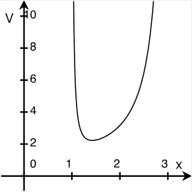
Figure 1: Plot of potential $V_{\rm eff,ext}(x)$, defined in (3.7), in terms of $x$.

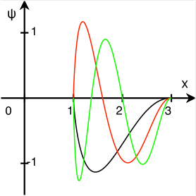
Figure 2: Plot of wavefunctions $\psi_{0}(x)$ (black line), $\psi_{1}(x)$ (red line), and $\psi_{2}(x)$ (green line) for potential (3.7) in terms of $x$.

Let us now sketch more involved extensions of $V_{\rm eff}(x)$, obtained from the rational extensions of Scarf I potential related to $X_{2}$-Jacobi EOPs [29]. The latter belong to three different types, where in all cases $U_{\rm ext}(u)$ can be written as shown in (3.1) with

$$U_{\rm rat}(u)=\frac{N_{1}(u)}{D(u)}+\frac{N_{2}(u)}{[D(u)]^{2}}.$$ (3.11)

Here

$$\begin{split}N_{1}(u)&=-4\left[(2A-1)(2B-1)(2B-2)\sin u+2(2A-1)^{2}-(2B-2)^{2}(2B+1)\right],\\ N_{2}(u)&=-8(2B-2)(2A-2B+1)(2A+2B-3)\\ &\quad\times\left[2(2A-1)(2B-1)\sin u-(2A-1)^{2}-2B(2B-2)\right],\\ D(u)&=(2B-1)\left[(2B-2)\sin u-(2A-1)\right]^{2}-(2A-2B+1)(2A+2B-3),\end{split}$$ (3.12)

for type I (with $1<B<A-1$),

$$\begin{split}N_{1}(u)&=-4\left[(2A-1)(2B+1)(2B+2)\sin u-2(2A-1)^{2}-(2B+2)^{2}(2B-1)\right],\\ N_{2}(u)&=8(2B+2)(2A-2B-3)(2A+2B+1)\\ &\quad\times\left[2(2A-1)(2B+1)\sin u-(2A-1)^{2}-2B(2B+2)\right],\\ D(u)&=(2B+1)\left[(2B+2)\sin u-(2A-1)\right]^{2}+(2A-2B-3)(2A+2B+1),\end{split}$$ (3.13)

for type II (with $0<B<A-\frac{3}{2}$), and

$$\begin{split}N_{1}(u)&=-8\left[B(2A-2)(2A-3)\sin u-A(2A-3)^{2}+4B^{2}\right],\\ N_{2}(u)&=8(2A-3)(2A-2B-3)(2A+2B-3)\\ &\quad\times\left[4B(2A-2)\sin u-4B^{2}-(2A-1)(2A-3)\right],\\ D(u)&=(2A-2)\left[(2A-3)\sin u-2B\right]^{2}+(2A-2B-3)(2A+2B-3),\end{split}$$ (3.14)

for type III (with $0<B<A-\frac{3}{2}$).

By proceeding as above, we obtain that in (3.5), $V_{\rm eff,rat}(x)$ is given by

$$V_{\rm eff,rat}(x)=\frac{{\cal N}_{1}(x)}{{\cal D}(x)}+\frac{{\cal N}_{2}(x)}{[{\cal D}(x)]^{2}},$$ (3.15)

where

$$\begin{split}{\cal N}_{1}(x)&=\frac{8}{ab(b-a)^{2}}\bigl{\{}\omega ab(\omega ab-1)(\omega ab-2)[(a+b)x-2ab]-\omega^{2}a^{2}b^{2}(a+b)^{2}\\ &\quad-(\omega ab-2)(b-a)^{2}\bigr{\}},\\ {\cal N}_{2}(x)&=\frac{128\omega}{(b-a)^{4}}(\omega ab-2)\big{[}\omega^{2}a^{3}b^{3}+(\omega ab-1)(b-a)^{2}\big{]}\\ &\quad\times\big{[}(a+b)(\omega ab-1)x-ab(\omega ab-2)\big{]},\\ {\cal D}(x)&=\frac{4}{(b-a)^{2}}\bigl{\{}(\omega ab-1)[(\omega ab-2)x+2a][(\omega ab-2)x+2b]-\omega^{2}a^{3}b^{3}\bigr{\}},\end{split}$$ (3.16)

for type I (with $\omega ab>\max\left(2,\frac{b-a}{2a}\right)$),

$$\begin{split}{\cal N}_{1}(x)&=\frac{8}{ab(b-a)^{2}}\bigl{\{}\omega ab(\omega ab+1)(\omega ab+2)[(a+b)x-2ab]+\omega^{2}a^{2}b^{2}(a+b)^{2}\\ &\quad-(b-a)^{2}(\omega ab+2)\bigr{\}},\\ {\cal N}_{2}(x)&=\frac{128\omega}{(b-a)^{4}}(\omega ab+2)\big{[}\omega^{2}a^{3}b^{3}-(\omega ab+1)(b-a)^{2}\big{]}\\ &\quad\times\big{[}-(a+b)(\omega ab+1)x+ab(\omega ab+2)\big{]},\\ {\cal D}(x)&=\frac{4}{(b-a)^{2}}\bigl{\{}(\omega ab+1)\big{[}(\omega ab+2)x-2a\big{]}\big{[}(\omega ab+2)x-2b\big{]}+\omega^{2}a^{3}b^{3}\bigr{\}},\end{split}$$ (3.17)

for type II (with $\omega ab>\frac{b-a}{a}$), and

$$\begin{split}{\cal N}_{1}(x)&=-\frac{8}{ab(b-a)^{3}}\bigl{\{}-\omega ab\big{[}\omega ab(a+b)-(b-a)\big{]}\big{[}\omega ab(a+b)-2(b-a)\big{]}x\\ &\quad+\big{[}\omega ab(a+b)-2(b-a)\big{]}(b-a)^{2}+\omega^{2}a^{2}b^{2}(b-a)^{3}\bigr{\}},\\ {\cal N}_{2}(x)&=\frac{128\omega}{(b-a)^{5}}\big{[}\omega ab(a+b)-2(b-a)\big{]}\bigl{\{}\omega^{2}a^{3}b^{3}-(b-a)\big{[}\omega ab(a+b)-(b-a)\big{]}\bigr{\}}\\ &\quad\times\bigl{\{}-\big{[}\omega ab(a+b)-(b-a)\big{]}x+\omega a^{2}b^{2}\bigr{\}},\\ {\cal D}(x)&=\frac{4}{(b-a)^{5}}\bigl{\{}\big{[}\omega ab(a+b)-(b-a)\big{]}\big{[}\big{(}\omega ab(a+b)-2(b-a)\big{)}x-2\omega a^{2}b^{2}\\ &\quad+2a(b-a)\big{]}\big{[}\big{(}\omega ab(a+b)-2(b-a)\big{)}x-2\omega a^{2}b^{2}+2b(b-a)\big{]}\\ &\quad+\omega^{2}a^{3}b^{3}(b-a)^{3}\bigr{\}},\end{split}$$ (3.18)

for type III (with $\omega ab>\frac{b-a}{a}$). The corresponding spectrum is given by (2.3), where $n$ runs over $n=0$, 1, 2,… in the type I and II cases, and over $n=-2$, 1, 2,… in the type III one.

As examples, for $\omega=a=1$, $b=3$, we obtain

$$\begin{split}V_{\rm eff,ext}(x)&=\frac{3x^{2}}{4(x-1)(3-x)}+\frac{16(3x-23)}{3(2x^{2}+16x-3)}+\frac{280(8x-3)}{(2x^{2}+16x-3)^{2}},\\ V_{\rm eff,ext}(x)&=\frac{3x^{2}}{4(x-1)(3-x)}+\frac{8(60x-59)}{15(20x^{2}-32x+15)}-\frac{88(16x-15)}{5(20x^{2}-32x+15)^{2}},\\ V_{\rm eff,ext}(x)&=\frac{3x^{2}}{4(x-1)(3-x)}+\frac{2(30x-13)}{3(20x^{2}-50x+33)}-\frac{14(10x-9)}{(20x^{2}-50x+33)^{2}},\end{split}$$ (3.19)

for type I, II, and III, respectively.

4 Conclusion

In the present paper, we have first shown that the PDM model of Ref. [34] can be alternatively solved by applying a PCT to the constant-mass Schrödinger equation for the Scarf I potential.

In a second step, on starting from the known rational extension of the latter connected with $X_{1}$-Jacobi EOPs, we have built a rationally-extended PDM model with the same spectrum as the starting model and wavefunctions expressed in terms of $X_{1}$-Jacobi EOPs instead of Jacobi polynomials.

Finally, we have sketched how some more involved PDM models may be obtained by starting from the rationally-extended Scarf I potentials related to $X_{2}$-Jacobi EOPs.

Data availability statement

No new data were created or analyzed in this study.

References

• [1] Bastard G 1988 Wave Mechanics Applied to Semiconductor Heterostructures (Les Ulis: Editions de Physique)
• [2] Weisbuch C and Vinter B 1997 Quantum Semiconductor Heterostructures (New York: Academic)
• [3] Serra L and Lipparini E 1997 Spin response of unpolarized quantum dots Europhys. Lett. 40 667
• [4] Harrison P and Valavanis A 2016 Quantum Wells, Wires and Dots: Theoretical and Computational Physics of Semiconductor Nanostructures (Chichester: Wiley)
• [5] Barranco M, Pi M, Gatica S M, Hernández E S and Navarro J 1997 Structure and energetics of mixed 4He-3He drops Phys. Rev. B 56 8997
• [6] Geller M R and Kohn W 1993 Quantum mechanics in crystals with graded composition Phys. Rev. Lett. 70 3103
• [7] Arias de Saavedra F, Boronat J, Polls A and Fabrocini A 1994 Effective mass of one 4He atom in liquid 3He Phys. Rev. B 50 4248(R)
• [8] Puente A, Serra L and Casas M 1994 Dipole excitation of Na clusters with a non-local energy density functional Z. Phys. D 31 283
• [9] Ring P and Schuck P 1980 The Nuclear Many Body Problem (New York: Springer)
• [10] Bonatsos D, Georgoudis P E, Lenis D, Minkov N and Quesne C 2011 Bohr Hamiltonian with a deformation-dependent mass term for the Davidson potential Phys. Rev. C 83 044321
• [11] Willatzen W and Lassen B 2007 The BenDaniel-Duke model in general nanowire structures J. Phys.: Condens. Matter 19 136217
• [12] Chamel N 2006 Effective mass of free neutrons in neutron star crust Nucl. Phys. A 773 263
• [13] Quesne C and Tkachuk V M 2004 Deformed algebras, position-dependent effective mass and curved spaces: An exactly solvable Coulomb problem J. Phys. A: Math. Gen. 37 4267
• [14] Schrödinger E 1940 A method of determining quantum-mechanical eigenvalues and eigenfunctions Proc. R. Ir. Acad. A46 9
• [15] Kalnins E G, Miller Jr W and Pogosyan G S 1996 Superintegrability and associated polynomial solutions: Euclidean space and the sphere in two dimensions J. Math. Phys. 37 6439
• [16] Kalnins E G, Miller Jr W and Pogosyan G S 1997 Superintegrability on the two-dimensional hyperboloid J. Math. Phys. 38 5416
• [17] Kempf A 1994 Uncertainty relation in quantum mechanics with quantum group symmetry J. Math. Phys. 35 4483
• [18] Hinrichsen H and Kempf A 1996 Maximal localization in the presence of minimal uncertainties in positions and in momenta J. Math. Phys. 37 2121
• [19] Witten E 1996 Reflections on the fate of spacetime Phys. Today 49 24
• [20] Bagchi B, Banerjee A, Quesne C and Tkachuk V M 2005 Deformed shape invariance and exactly solvable Hamiltonians with position-dependent effective mass J. Phys. A: Math. Gen. 38 2929
• [21] Quesne C 2006 First-order intertwining operators and position-dependent mass Schrödinger equations in $d$ dimensions Ann. Phys., NY 321 1221
• [22] Bagchi B, Gorain P, Quesne C and Roychoudhury R 2004 A general scheme for the effective-mass Schrödinger equation and the generation of the associated potentials Mod. Phys. Lett. A 19 2765
• [23] Quesne C 2009 Point canonical transformation versus deformed shape invariance for position-dependent mass Schrödinger equations SIGMA 5 046
• [24] Quesne C 2021 Comment on ‘Exact solution of the position-dependent effective mass and angular frequency Schrödingert equation: harmonic oscillator model with quantized confinement parameter’ J. Phys. A: Math. Theor. 54 368001
• [25] Quesne C 2022 Generalized semiconfined harmonic oscillator model with a position-dependent effective mass Eur. Phys. J. Plus 137 225
• [26] Quesne C 2023 Semi-infinite quantum wells in a position-dependent mass background Quantum Stud.: Math. Found. 10 237
• [27] Gómez-Ullate D, Kamran N and Milson R 2009 An extended class of orthogonal polynomials defined by a Sturm-Liouville problem J. Math. Anal. Appl. 359 352
• [28] Quesne C 2008 Exceptional orthogonal polynomials, exactly solvable potentials and supersymmetry J. Phys. A: Math. Theor. 41 392001
• [29] Quesne C 2009 Solvable rational potentials and exceptional orthogonal polynomials in supersymmetric quantum mechancics SIGMA 5 084
• [30] Odake S and Sasaki R 2009 Infinitely many shape invariant potentials and new orthogonal polynomials Phys. Lett. B 679 414
• [31] Gómez-Ullate D, Kamran N and Milson R 2012 Two-step Darboux transformations and exceptional Laguerre polynomials J. Math. Anal. Appl. 387 410
• [32] Odake S and Sasaki R 2011 Exactly solvable quantum mechanics and infinite families of multi-indexed orthogonal polynomials Phys. Lett. B 702 164
• [33] Quesne C 2016 Quantum oscillator and Kepler-Coulomb problems in curved spaces: Deformed shape invariance, point canonical transformations, and rational extensions J. Math. Phys. 57 102101
• [34] Jafarov E I and Nagiyev S M 2022 Exact solution of the position-dependent mass Schrödinger equation with the completely positive oscillator-shaped quantum well potential arXiv:2212.13062
• [35] BenDaniel D J and Duke C B 1966 Space-charge effects on electron tunneling Phys. Rev. 152 683
• [36] von Roos O 1983 Position-dependent effective masses in semiconductor theory Phys. Rev. B 27 7547
• [37] Zhu Q-G and Kroemer H 1983 Interface connection rules for effective-mass wave functions at an abrupt heterojunction between two different semiconductors Phys. Rev. B 27 3519
• [38] Mustafa O and Mazharimousavi S H 2007 Ordering ambiguity revisited via position-dependent mass pseudo-momentum operators Int. J. Theor. Phys. 46 1786
• [39] Mustafa O and Alghadi Z 2019 Position-dependent mass momentum operator and minimal coupling: point canonical transformation and isospectrality Eur. Phys. J. Plus 134 228
• [40] Gómez-Ullate D, Marcellán F and Milson R 2013 Asymptotic and interlacing properties of zeros of exceptional Jacobi and Laguerre polynomials J. Math. Anal. Appl. 399 480
• [41] Liaw C, Littlejohn L and Stewart Kelly J 2015 Spectral analysis for the exceptional $X_{m}$-Jacobi equation Electron. J. Differential Equations 2015 194
• [42] Bonneux N 2019 Exceptional Jacobi polynomials J. Approx. Theory 239 72