2D-3D Pose Tracking with Multi-View Constraints

Abstract

Camera localization in 3D LiDAR maps has gained increasing attention due to its promising ability to handle complex scenarios, surpassing the limitations of visual-only localization methods. However, existing methods mostly focus on addressing the cross-modal gaps, estimating camera poses frame by frame without considering the relationship between adjacent frames, which makes the pose tracking unstable. To alleviate this, we propose to couple the 2D-3D correspondences between adjacent frames using the 2D-2D feature matching, establishing the multi-view geometrical constraints for simultaneously estimating multiple camera poses. Specifically, we propose a new 2D-3D pose tracking framework, which consists: a front-end hybrid flow estimation network for consecutive frames and a back-end pose optimization module. We further design a cross-modal consistency-based loss to incorporate the multi-view constraints during the training and inference process. We evaluate our proposed framework on the KITTI and Argoverse datasets. Experimental results demonstrate its superior performance compared to existing frame-by-frame 2D-3D pose tracking methods and state-of-the-art vision-only pose tracking algorithms. More online pose tracking videos are available at https://youtu.be/yfBRdg7gw5M.

I Introduction

Camera localization in 3D LiDAR maps has attracted more and more attention due to the convenient system setup and high application prospects for mobile robots and autonomous driving. On the one hand, it only leverages lightweight and low-cost cameras, similar to visual SLAM, while offering significant potential in mitigating pose drift issues. On the other hand, LiDAR maps can be effortlessly constructed at a large scale and remain unaffected by changes in illumination, thanks to LiDAR SLAM or registration techniques. However, the existence of cross-modal gaps between camera images and LiDAR point clouds hampers the establishment of robust 2D-3D correspondences, consequently challenging the robustness and accuracy of camera localization.

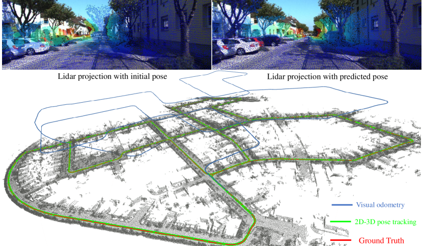
Figure 1: Illustrative examples of the proposed 2D-3D pose tracking and visual odometry on the KITTI 00 sequence. Top: The visualization of the LiDAR projection with initial pose and predicted pose. Bottom: The top view of the final trajectories of the proposed method and the visual odometry algorithm.

To alleviate the issue of cross-modal gaps, traditional methods mainly use geometric consistency in 3D or 2D space[1, 2, 3, 4, 5]. The localization performance highly depends on the accuracy of intermediary “products” such as reconstructed sparse points or 3D line segments, which lack robustness and generalization capability. With the help of deep learning, the correspondences between LiDAR points and images are established by a cross-modal flow network[6, 7], and then the camera poses can be inferred using the PnP solver in a RANSAC loop. Besides, some methods also utilize a neural network to regress the camera poses directly[8, 9, 10]. Despite their remarkable performance, these methods solely estimate the camera pose frame by frame, disregarding the multi-view constraints between adjacent frames, thereby resulting in an unstable pose tracking.

We notice that the bundle adjustment of multi-view image matching can ensure the smoothness of camera pose estimation in classical visual odometry algorithms, and 2D-2D image matching is already a mature technique with traditional handcraft features and learning-based optical flow. Therefore, our intuition is to fuse the LiDAR-image correspondences and image-image flow to establish multi-view visual constraints for further smoothing and improving localization performance.

In this paper, we propose a novel 2D-3D pose tracking framework that leverages multi-view constraints to achieve accurate pose estimation for consecutive frames. The proposed framework formulates pose estimation as a local optimization problem with an initial pose. Specifically, the initial pose of each frame is from the previous frame during pose tracking. We impose a random disturbance on the ground truth poses to obtain the initial poses during network training. The 3D point clouds are projected onto the 2D plane with rough initial poses to obtain the synthetic depth maps. Then we utilize a hybrid flow estimation network to estimate the image-to-LiDAR depth flows between the adjacent camera frames and a synthetic depth map, as well as the optical flow between the adjacent camera frames. Especially, a cross-modal consistency loss function is devised to incorporate multi-view constraints between the estimated image-to-LiDAR depth flows and the optical flow into the learning process. During pose tracking, we define an objective function consisting of the reprojection error and the cross-modal consistency error, and then optimize the estimated camera poses under the paradigm of a non-linear least square problem. An illustrative example of the proposed framework and visual odometry is shown in Fig. 1.

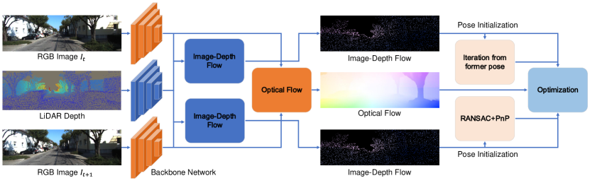
Figure 2: The proposed 2D-3D pose tracking framework. It consists of two main components: the front-end hybrid flow estimation network, and the back-end pose optimization module.

Our main contribution can be summarized as:

• We propose an effective hybrid flow estimation network that simultaneously estimates image-to-LiDAR depth flow and image-to-image flow between consecutive video frames. We further devise a cross-modal consistency loss function to incorporate multi-view constraints into the learning process.

• We introduce a back-end optimization algorithm to smooth and improve localization performance of camera pose tracking in LiDAR maps. The estimated poses corresponding to the consecutive frames are refined together under the paradigm of a non-linear least square problem based on cross-modal consistency.

• We conduct extensive experiments on two public datasets (i.e., KITTI and Argoverse) to evaluate the performance. The experimental results demonstrate that the proposed 2D-3D pose tracking framework can achieve more accurate and robust localization than other frame-by-frame pose tracking methods.

II Related Work

II-A Visual-only Pose Tracking

Cameras provide a wealth of spectral and degenerated geometrical information at a significantly lower cost compared to other competing sensor options. As a result, visual localization plays an important role in modern localization systems for autonomous vehicles. The paradigm of visual localization is to fetch 2D-2D correspondences between two or more 2D images, typically employing techniques such as optical flow or feature-based matching, and then leverage the epipolar geometry to compute the relative motion. To overcome problems such as scale ambiguity and error accumulation, Triggs [11] introduces a joint optimization procedure that minimizes the re-projection error between the observed feature points and the estimated points, which is called bundle adjustment optimization. It adjusts the bundle of rays passing through the camera center and the feature points in the 3D world to minimize this error over multiple frames. In addition, some methods [12, 13, 14, 15] propose to incorporate global information, such as GPS or inertial measurement units (IMUs), to help resolve scale ambiguity and reduce error accumulation during pose tracking. In recent years, with the advent of machine learning and particularly deep learning, learned visual pose tracking methods [16, 17, 18, 19] have also emerged. These methods leverage Convolutional Neural Networks (CNNs) to learn features and their associations between frames, thereby estimating camera poses. However, visual-only pose tracking has inevitable pose drift and lacks robustness over challenging conditions such as illumination, weather, and season changes over time.

II-B 2D-3D Pose Tracking

Unlike cameras, LiDAR is less susceptible to those visual factors. Therefore, pose tracking based on 2D-3D correspondences between 2D images and offline 3D LiDAR maps holds greater potential in achieving robust localization. Existing approaches focus on solving the cross-modal gaps between 2D images and 3D LiDAR points. Some researchers propose to extract repeatable points or line features from images and LiDAR points for 2D-3D matching [20, 21, 4, 5], which achieve remarkable performance in scenes with rich geometric information. Other approaches transform data into the same modal at first. For example, in certain approaches [1, 2, 3], sparse 3D points are reconstructed from consecutive camera frames or stereo disparity images captured by a stereo camera. Subsequently, these reconstructed points are matched with the global LiDAR map. The localization performance of these approaches relies on the accuracy of the reconstructed 3D points. In addition, the 3D reconstruction process is time-consuming and the reconstructed 3D points may not correspond to any points in the LiDAR map. Other approaches [6, 22, 23, 8, 9, 7, 10] first project the LiDAR map onto the 2D plane to obtain synthetic depth maps and then match them with camera images. However, these methods predict the camera pose frame by frame and ignore the constraints between adjacent frames. As a result, they are prone to jitter and encounter error accumulation problems during pose tracking. [24] implicitly utilizes the temporal features between consecutive frames, but still predicts the camera poses frame by frame. In this paper, we propose a novel 2D-3D pose tracking framework which integrates the multi-view constraints between consecutive frames during the network training and inference. Unlike the aforementioned methods, we regard the poses of multiple frames as a whole and optimize them together under the proposed cross-modal consistency, thus can well handle the cross-modal differences and multi-view constraints.

III Proposed Method

The general frame-by-frame 2D-3D pose tracking framework adheres to the paradigm of local optimization based on an initial pose, which can be formulated as follows: In the beginning, the camera pose of the first frame is initialized using GPS. For each subsequent camera frame, the pose of the previous frame serves as the initial estimation. Based on this initial pose, a fixed-size point cloud is segmented from the global LiDAR map. Then, the 2D-3D correspondences between the camera frame and the segmented point cloud are estimated. Finally, the corresponding camera pose is calculated using the PnP solver. Previous work[8, 9, 7] has confirmed the feasibility of this paradigm for pose tracking. However, it has also highlighted the limited robustness in some scenarios, such as environments with extreme degeneracy. The unstable camera localization motivates us to incorporate multi-view constraints between adjacent camera frames into the 2D-3D pose tracking framework.

Our proposed 2D-3D pose tracking framework is shown in Fig. 2. Our key insight is to simultaneously estimate the 6-DoF poses for two adjacent frames based on a hybrid flow estimation network. For each group of two adjacent frames, we initialize the poses as the same and from the estimation of previous continuous frames. Then the global LiDAR maps are cropped with a fixed size centered at the initial poses. By using the hybrid 2D-3D and 2D-2D flow network, we can obtain stable 2D-3D correspondences. PnP solver is then utilized to get the estimated poses. Finally, these poses are further refined using a back-end optimization algorithm that incorporates multi-view constraints. Subsequently, the initial pose of the current time step is updated with the estimated pose of the current frame, while the estimated pose of the next frame serves as the initial pose for the next time step.

In the following, we first introduce the front-end flow estimation network, and then describe the details of the proposed cross-modal consistency loss function. Finally, we present the back-end optimization algorithm.

III-A Hybrid Flow Estimation Network

III-A1 Depth Map Generation

To obtain the image-to-LiDAR depth flow using the flow estimation network, we first need to project the 3D LiDAR point clouds to the 2D plane to generate the synthetic depth maps. The projection process follows the pinhole camera model which can be described as:

$$\left(\begin{array}[]{l}u\\ v\\ 1\end{array}\right)=\frac{1}{Z}\left(\begin{array}[]{ccc}f_{x}&0&c_{x}\\ 0&f_{y}&c_{y}\\ 0&0&1\end{array}\right)\left(\begin{array}[]{l}X\\ Y\\ Z\end{array}\right)\triangleq\frac{1}{Z}\bm{K}P$$ (1)

where $(X\quad Y\quad Z)^{T}$ and $P$ represent the coordinates of the 3D points in the camera coordinate system. $(u\quad v\quad 1)^{T}$ represents the homogeneous coordinates of the projection in the pixel coordinate system. The intrinsic camera parameters, $f_{x},f_{y},c_{x},c_{y}$, form the camera matrix $\bm{K}$. Additionally, the occlusion removal scheme proposed by [25] is applied to eliminate occluded 3D points on the generated depth map.

III-A2 Flow Estimation

After obtaining the synthetic depth map, we utilize a hybrid flow estimation network to predict the image-to-LiDAR depth flow and the optical flow between the consecutive camera frames simultaneously. The hybrid network mainly consists of three parts: the image-to-LiDAR depth flow estimation networks $F_{c}$ and $F_{n}$, and the optical flow estimation network $F_{i}$. We use I2D-Loc[7] as the backbone to predict the image-to-LiDAR depth flow and RAFT[26] as the backbone to predict the optical flow because they both excel at their respective tasks.

The ground truth image-to-LiDAR depth flow is generated by computing the distance between the LiDAR depth maps projected based on the initial pose and the ground truth pose. Given the initial pose $\bm{T}_{\text{init}}$, the ground truth image-to-LiDAR depth flow for the current frame can be computed using the following formulation:

$${[\Delta u,\Delta v]_{\text{cur2depth}}=h\left(P_{w},\hat{\bm{T}}_{\text{cur}}\right)-h\left(P_{w},\bm{T}_{\text{init}}\right)}$$ (2)

$$h(P,\bm{T})\triangleq\bm{KT}P$$ (3)

where $[\Delta u,\Delta v]_{\text{cur2depth}}$ is the calculated ground truth image-to-LiDAR depth flow between the current camera frame and the synthetic depth map. $\hat{\bm{T}}_{\text{cur}}$ and $\bm{T}_{\text{init}}$ are the ground truth pose and the initial pose, respectively. $P_{w}$ is the coordinate of the corresponding 3D point cloud in the world coordinate system. $h$ represents the camera projection function that first transforms 3D points from the world coordinate system to the camera coordinate system and then projects them to the 2D plane. Besides, the ground truth image-to-LiDAR depth flow for the next frame can be calculated based on a similar formulation:

$${[\Delta u,\Delta v]_{\text{next2depth}}=h\left(P_{w},\hat{\bm{T}}_{\text{next}}\right)-h\left(P_{w},\bm{T}_{\text{init}}\right)}$$ (4)

where $[\Delta u,\Delta v]_{\text{next2depth}}$ represents the calculated ground truth image-to-LiDAR depth flow between the next camera frame and the synthetic depth map. $\hat{\bm{T}}_{\text{next}}$ is the ground truth pose of the next camera frame.

III-B Loss Function

Regarding the network supervision, we first consider the masked average endpoint error (EPE) between the predicted image-to-LiDAR depth flow and the ground truth, defined as follows:

$$L_{\text{epe}}=\frac{\sum g(u,v)\left\|f_{\text{pre}}(u,v)-f_{\text{gt}}(u,v)\right\|_{2}}{\sum g(u,v)}$$ (5)

$$g(u,v)=\left\{\begin{array}[]{l}1,f_{\text{gt}}\neq 0\\ 0,\text{otherwise}\end{array}\right.$$ (6)

where $f_{\text{pre}}$ and $f_{\text{gt}}$ represent the predicted and ground truth image-to-LiDAR depth flow, respectively. $g(u,v)$ identifies the valid pixels in the ground truth image-to-LiDAR depth flow. Due to the superior accuracy achieved by the same modal image optical flow network compared to the image-to-LiDAR depth flow network, we load a pre-trained optical flow model and keep its parameters fixed during network training.

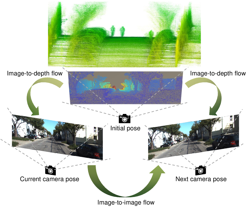
Figure 3: Diagram of the cross-modal consistency.

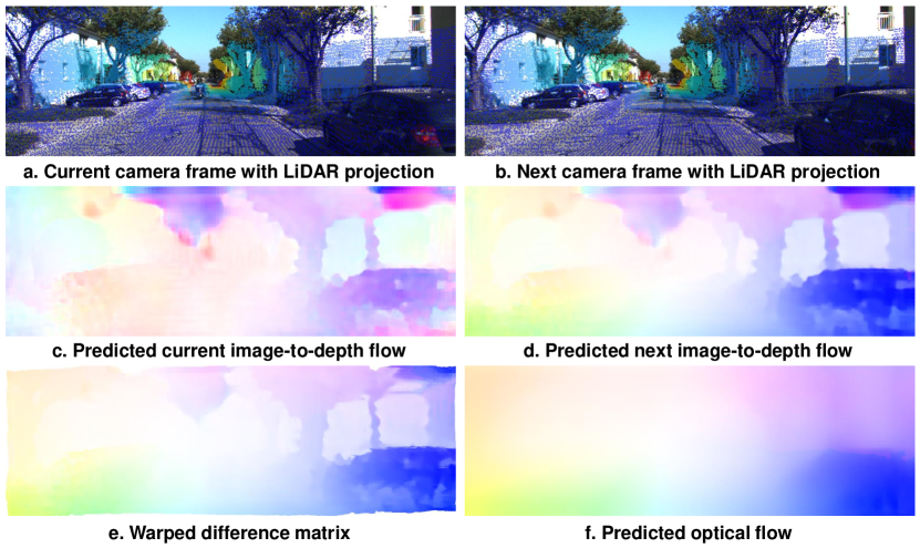
Figure 4: Visualization of the flow estimation. a: LiDAR projection overlay on the current camera image. b: LiDAR projection overlay on the next camera image. c: Predicted image-to-LiDAR depth flow between the current image and the LiDAR projection. d: Projected image-to-LiDAR depth flow between the next image and the LiDAR projection. e: Warped difference matrix between the predicted image-to-depth flows. f: Predicted optical flow between the two camera images.

Additionally, to incorporate the multi-view constraints between two adjacent camera frames during the network training, we propose a cross-modal consistency-based loss function, which is formulated as follows:

$$L_{\text{consist}}=\left\|w\left(f_{\text{pre}}^{\text{n2d}}-f_{\text{pre}}^{\text{c2d}},f_{\text{pre}}^{\text{c2d}}\right)-f_{\text{pre}}^{\text{c2n}}\right\|_{2}$$ (7)

where $f_{\text{pre}}^{\text{n2d}}$ represents the predicted image-to-LiDAR depth flow between the next camera frame and the synthetic depth map. Similarly, $f_{\text{pre}}^{\text{c2d}}$ represents the predicted image-to-LiDAR depth flow for the current camera frame. $f_{\text{pre}}^{\text{c2n}}$ is the predicted optical flow between the adjacent camera frames. $w$ represents the warping operation.

The cross-modal consistency, as shown in Fig. 3, explicitly describes the relationship between the adjacent camera frames and the synthetic depth map. Specifically, the image-to-depth flow represents the 2D-3D correspondences between the camera frame and depth map. Fig. 4c and 4d visualize the predicted flows corresponding to the current and next frame, respectively. The image-to-image flow (i.e. optical flow) represents the 2D-2D correspondences between two adjacent camera frames, which is shown in Fig. 4f. By calculating the difference between the predicted image-to-depth flows, we will obtain the equivalent image-to-image flow between the camera frames. As a result, the error between the equivalent and predicted image-to-image flow constructs the multi-view constraints between these predictions. In addition, it’s important to note that the predicted image-to-LiDAR depth flow represents the displacement field from the synthetic depth map to the image. Hence, the difference between the image-to-LiDAR depth flows of two adjacent frames is not equivalent to the image-to-image flow between them. We need to warp the calculated difference matrix based on the image-to-LiDAR depth flow of the first frame to obtain the final equivalent optical flow.

The final loss function is the sum of the above loss functions:

$$L=L_{\text{epe}}^{\text{cur}}+L_{\text{epe}}^{\text{next}}+L_{\text{consist}}$$ (8)

where $L_{\text{epe}}^{\text{cur}}$ is the average endpoint error of the predicted current image-to-depth flow. $L_{\text{epe}}^{\text{next}}$ is the average endpoint error of the predicted next image-to-depth flow.

In summary, we employ two loss functions to guide the network training: the average endpoint error and the cross-modal consistency loss function. The average endpoint error serves as a conventional constraint commonly used in optical flow estimation tasks. The cross-modal consistency error introduces the multi-view constraints between adjacent camera frames, capturing the relationship between different views.

III-C Multi-View Constraints-based Back-End Optimization

During pose tracking, as previously mentioned, we utilize the trained hybrid flow estimation network to simultaneously predict the image-to-LiDAR depth flows between the adjacent camera frames and the synthetic depth map, as well as the optical flow between the camera frames. Then the camera poses corresponding to the two camera frames are solved using the PnP solver according to the prediction. Besides, we define an energy function to further optimize the solved poses, as:

$$\bm{T}_{\text{cur}}^{*},\bm{T}_{\text{next}}^{*}=\operatorname*{arg\,min}_{\bm{T}_{\text{cur}},\bm{T}_{\text{next}}}(E_{\text{consist}}+E_{\text{reproj}}^{\text{cur}}+E_{\text{reproj}}^{\text{next}}),$$ (9)

where $\bm{T}_{\text{cur}}$ and $\bm{T}_{\text{next}}$ represent the predicted camera poses corresponding to the current and next frames, respectively. $E_{\text{consist}}$ is the cross-modal consistency error and formulated as follows:

$$E_{\text{consist}}=\left\|h(P_{w},\bm{T}_{\text{next}})-h(P_{w},\bm{T}_{\text{cur}})-f^{\text{c2n}}_{\text{pre}}\right\|_{2}$$ (10)

where $h$ is the camera projection function and defined as Eq. (3). $f^{\text{c2n}}_{\text{pre}}$ is the predicted optical flow. Based on this formula, we begin by projecting the 3D points onto the 2D plane using the predicted poses. Subsequently, we compute the difference matrix between the projections to derive the equivalent optical flow. Therefore, $E_{\text{consist}}$ represents the distance between the equivalent and predicted optical flows. Additionally, $E_{\text{reproj}}^{\text{cur}}$ and $E_{\text{reproj}}^{\text{next}}$ both represent the reprojection error of the solved camera poses:

$$E_{\text{reproj}}^{\text{cur}}=\left\|h(P,\bm{T}_{\text{cur}})-X_{\text{cur}}\right\|_{2}$$ (11)

$$E_{\text{reproj}}^{\text{next}}=\left\|h(P,\bm{T}_{\text{next}})-X_{\text{next}}\right\|_{2}$$ (12)

where $X_{\text{cur}}$ and $X_{\text{next}}$ represent the 2D coordinates of pixels with valid depth values in the depth maps that have been warped using the predicted image-to-LiDAR depth flows.

Based on the formulated energy function, we employ the least square method to determine the optimal camera poses $\bm{T}_{\text{cur}}^{*}$ and $\bm{T}_{\text{next}}^{*}$ that minimize the function value. The obtained $\bm{T}_{\text{cur}}^{*}$ replaces the initial pose $\bm{T}_{\text{init}}$ as the final pose for the current frame, while $\bm{T}_{\text{next}}^{*}$ is utilized to initialize the subsequent localization process.

IV Experiments

In this section, we conduct extensive experiments on two public datasets to evaluate the performance of our proposed method.

TABLE I: Performance comparison of the flow estimation network under different setups on the KITTI dataset. “C”, “N”, “T”, and “L” represent the current image-to-LiDAR depth flow estimation network $F_{c}$, the next image-to-LiDAR depth flow estimation network $F_{n}$, additional training, and the cross-modal consistency loss function, respectively. In (e) and (f), the first value represents the performance of the network $F_{c}$, while the second value represents the performance of the network $F_{n}$.

Case	Module				Mean Error		Median Error		Fail[%] $\downarrow$
	C	N	T	L	Rot.[∘] $\downarrow$	Transl.[cm] $\downarrow$	Rot.[∘] $\downarrow$	Transl.[cm] $\downarrow$
Initial pose					$\approx 9.6726$	$\approx 182.8381$	$\approx 9.9033$	$\approx 187.3079$	-
(a)	✓				0.8619	24.6955	0.6900	17.6687	1.81
(b)		✓			2.5284	75.4198	1.8364	63.5510	16.65
(c)	✓		✓		0.8375	22.4241	0.6777	15.3426	1.61
(d)		✓	✓		2.4225	74.0713	1.8184	62.6881	16.67
(e)	✓	✓	✓		0.8640/2.4801	23.7909/75.5822	0.6978/1.8511	16.0583/63.5162	1.61/16.93
(f)	✓	✓	✓	✓	0.9051/2.4842	26.5121/71.8964	0.7168/1.7970	17.8525/61.0808	1.78/15.90

IV-A Dataset and Evaluation Metrics

IV-A1 Dataset

We conduct experiments on KITTI[27] and Argoverse[28] datasets. KITTI is commonly used in the field of autonomous driving. It consists of 22 sequences. We use sequences 03, 05, 06, 07, 08, and 09 as the training set and sequences 00 and 10 as the validation set. Argoverse offers more complex driving scenarios, albeit with shorter odometry sequences. We use the sequences train1, train2, and train3 as the training set, and sample several sequences with less noise as the validation set.

To acquire the global LiDAR map, unavailable in the datasets, we begin by aggregating all scans based on the ground truth poses. Subsequently, to conserve storage space, we down-sample the aggregated map at a resolution of 0.1m. During training, we segment the point cloud for each frame by centering it around the ground truth pose and extending it 100m forward, 10m backward, and 25m to the left and right. During pose tracking, the coverage of the segmented point cloud remains fixed, but it is centered on the initial pose of the current frame being tracked.

IV-A2 Evaluation Metrics

We evaluate the performance of the proposed method in two ways. The first one is to evaluate the localization accuracy frame by frame using the mean and median errors of the predicted poses. Following [6], [7], we assume the position errors larger than four meters as a failure. The second one is to evaluate the pose tracking performance on the global LiDAR maps using the average trajectory error (ATE) and the relative pose error (RPE), which are defined in [29] and commonly used for quantitative trajectory evaluation.

IV-B Experimental Setup

Accounting for the varying sizes of RGB images across different sequences, we uniformly crop all RGB images to a resolution of $960\times 320$ during network training. As mentioned above, the proposed hybrid network comprises three components: the current image-to-LiDAR depth flow estimation network $F_{c}$, the next image-to-LiDAR depth flow estimation network $F_{n}$, and the optical flow estimation network $F_{i}$. We employ I2D-Loc[7] as the backbone for $F_{c}$ and $F_{n}$, while for $F_{i}$, we utilize RAFT-S[26] as the backbone due to memory limitations. In particular, we initialize $F_{c}$ and $F_{i}$ by loading the pre-trained models provided by [7, 26]. As for $F_{n}$, we first train it singly for 100 epochs based on the same experimental setup in [7]. Subsequently, we load all the pre-trained model weights and conduct joint training for additional 50 epochs on $F_{c}$, $F_{n}$, and $F_{i}$ using the proposed cross-modal consistency loss function. The learning rate, weight decay, and training batch size are set to $4\times 10^{-6}$, $1\times 10^{-4}$, and 2, respectively. We employ the MultiStepLR learning rate scheduler, which reduces the learning rate to one-tenth of the previous value at the 10th and 30th epochs. The joint training is performed using two NVIDIA RTX 3090 Ti GPUs, while the other experiments are conducted on a single NVIDIA RTX 3090 Ti GPU.

TABLE II: Pose tracking performance comparison on KITTI sequence 00. “Complete” indicates that the pose tracking process ends without any interruptions caused by localization failure. The localization errors are calculated until being interrupted.

Case	Method	Translation Error		Rotation Error		Complete	Param[M]	Time[ms]
		Mean.[cm] $\downarrow$	Std.[cm] $\downarrow$	Mean.[∘] $\downarrow$	Std.[∘] $\downarrow$
(a)	CMRNet[8]	205	107	126	39	✓	37.1	25
(b)	I2D-Loc[7]	21	10	0.46	0.30		6.3	176
(c)	VO	162	63	4.95	2.34	✓	-	219
(d)	I2D-VO	15	21	0.48	0.64	✓	6.3	180
(e)	Ours w/o Optim	14	17	0.50	0.53		13.6	374
(f)	Ours w/ Optim	14	17	0.49	0.54	✓	13.6	588

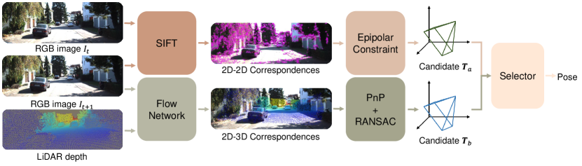
Figure 5: 2D-3D pose tracking framework that loosely couples 2D-3D correspondences and 2D-2D correspondences.

IV-C Ablation Study

In this section, we evaluate the effectiveness of the multi-view constraints during the training process. The experimental results are shown in Table I, where we report the mean and median errors of the calculated poses based on the predicted flows as evaluation metrics.

The performance of the single image-to-LiDAR depth flow estimation network for current and next frames using the official I2D-Loc model is displayed in Table I(a) and (b). The error range of the initial poses for the network $F_{n}$ is greater than that for the network $F_{c}$, resulting in a relatively higher localization accuracy for the network $F_{c}$. After conducting an additional 50 epochs of training for each network individually in Table I(c) and (d), the pose errors of the two networks both decrease by a little margin. Then when the networks $F_{c}$ and $F_{n}$ are trained jointly for another 50 epochs, Table I(e) shows that the localization accuracy for each network hasn’t been improved. The above experiments imply an inherent conflict between the network $F_{c}$ and $F_{n}$ due to their varying error ranges for initial poses. In Table I(f), we utilize the proposed cross-modal consistency loss function to incorporate the multi-view constraints during the training process. The experimental result shows that the localization performance of the network $F_{c}$ degrades a little, but the pose error of the network $F_{n}$ decreases by a large margin. This outcome demonstrates that the proposed cross-modal consistency-based loss bridges the gaps between the predicted 2D-3D correspondences of adjacent frames.

IV-D Results Analysis

Table II gives the quantitative results of our method evaluated on KITTI sequence 00. In addition to the frame-by-frame 2D-3D pose tracking methods CMRNet[8] and I2D-Loc[7], we also compare our method with the traditional visual odometry algorithm and a devised 2D-3D pose tracking framework that loosely couples the visual odometry algorithm with I2D-Loc, referred to as I2D-VO. As illustrated in Fig. 5, this framework utilizes the visual odometry algorithm and I2D-Loc to generate pose candidates based on 2D-2D and 2D-3D correspondences, respectively. Subsequently, the final pose is selected from these candidates based on predefined thresholds.

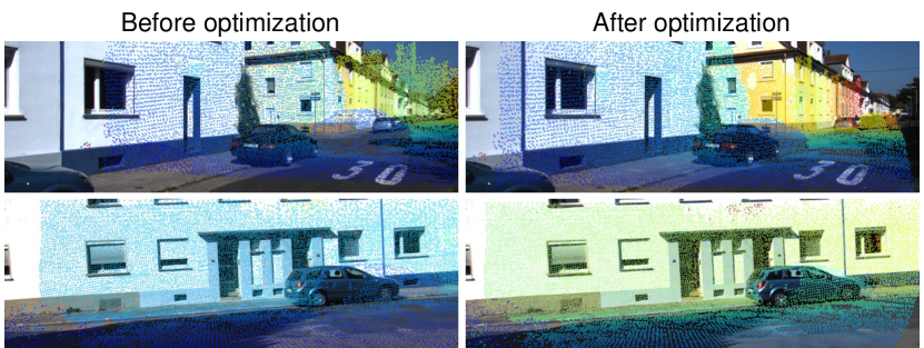
Figure 6: LiDAR projection overlaid on the next frame before and after optimization.

TABLE III: Performance comparison on KITTI dataset.

Method	KITTI_00 (1861m)				KITTI_10 (459m)				Arg_2c07 (44m)				Arg_2595 (54m)
	Transl.[m] $\downarrow$		Rot.[∘] $\downarrow$		Transl.[m] $\downarrow$		Rot.[∘] $\downarrow$		Transl.[m] $\downarrow$		Rot.[∘] $\downarrow$		Transl.[m] $\downarrow$		Rot.[∘] $\downarrow$
	Mean	Std	Mean	Std	Mean	Std	Mean	Std	Mean	Std	Mean	Std	Mean	Std	Mean	Std
VINS-Fusion[30]	16.70	9.40	4.99	2.51	2.34	1.13	1.75	0.74	3.09	2.24	22.87	6.77	19.02	11.04	176.67	1.11
I2D-VO	0.24	0.26	0.54	0.94	0.61	0.91	2.74	15.61	0.43	0.23	0.45	0.42	0.34	0.22	4.86	0.18
Ours	0.13	0.17	0.49	0.55	0.45	0.63	1.04	1.24	0.17	0.15	0.58	0.34	0.14	0.11	2.96	0.20

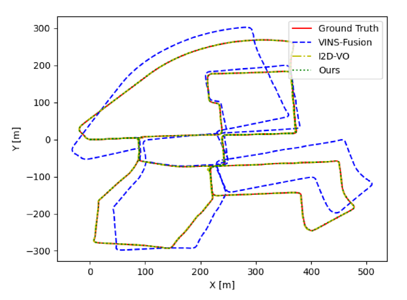
(a) KITTI_00

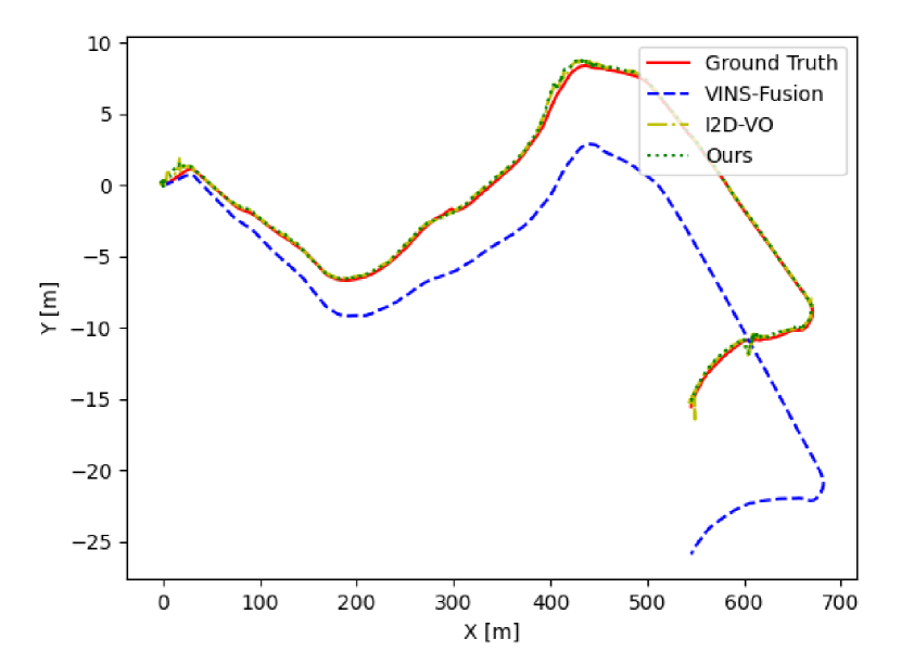
(b) KITTI_10

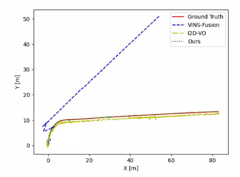
(c) Argoverse_2c07

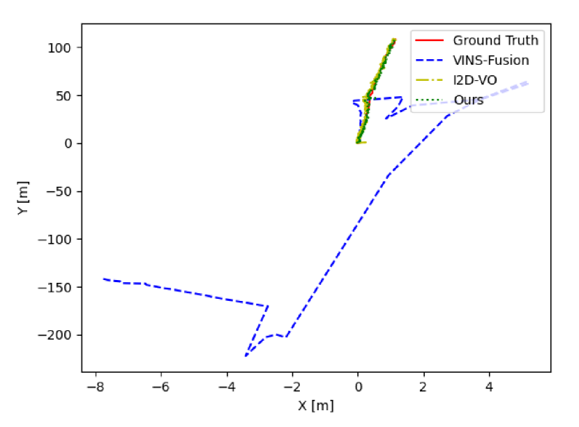
(d) Argoverse_2595

Figure 7: Estimated trajectories of three tested methods on four sampled LiDAR maps.

According to Table II(a) and (b), CMRNet efficiently tracks the entire LiDAR map without any interruption, albeit with certain limitations in its localization accuracy. Conversely, I2D-Loc boasts superior localization precision, yet it falls short of completing the entire map. This difference arises due to the heavy dependence of I2D-Loc on accurate 2D-3D correspondences, while CMRNet directly regresses camera poses. Additionally, as shown in Table II(c), the traditional visual odometry (VO) algorithm can track the entire map seamlessly. However, as shown in Fig. 1, the drift of VO is serious. By integrating I2D-Loc with the visual odometry algorithm in a loosely-coupled manner, our proposed framework, I2D-VO, accomplishes an enhancement in localization accuracy and successfully overcomes previous shortcomings. In Table II(e) and (f), our proposed 2D-3D pose tracking framework, which incorporates multi-view constraints, achieves minimal translation and rotation errors upon map completion. Furthermore, as demonstrated in Fig. 6, the accuracy of 2D-3D correspondences noticeably improves the following optimization in various challenging scenarios. In these cases, a single image-to-depth flow estimation network will fail to predict reliable 2D-3D correspondences due to homogeneous depth projections or extremely dark RGB images.

To highlight the outstanding performance of our proposed 2D-3D pose tracking methodology, we conducted a comprehensive comparison with the state-of-the-art visual-only pose tracking system, VINS-Fusion[30]. The evaluation was conducted on multiple sequences, including sequences 00 and 10 from the KITTI dataset, as well as sequences 2c07- and 2595- from the Argoverse dataset. The estimated trajectories of these sampled sequences are depicted in Fig. 7, demonstrating the excellent alignment of our proposed method with the ground truth trajectories.

Quantitative analysis, presented in Table III, provides clear evidence of the superiority of our proposed 2D-3D pose tracking method, which incorporates multi-view constraints. Across all four LiDAR maps, our method consistently outperforms the other tested methodologies, delivering remarkable performance.

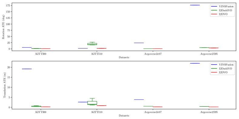
Figure 8: Comparison of ATE between VINS-Fusion and our proposed methods.

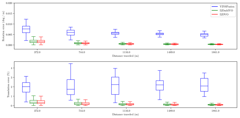
Figure 9: Comparison of RPE between VINS-Fusion and our proposed methods on the KITTI 00 sequence.

Additionally, we have also conducted a comparison between our proposed method and VINS-Fusion, utilizing Absolute Trajectory Error (ATE) and Relative Pose Error (RPE) as the key performance metrics. The quantitative outcomes are presented in Fig. 8 and Fig. 9. These figures emphatically demonstrate that our proposed method consistently achieves superior localization accuracy. Moreover, it exhibits reduced drift during pose tracking compared to both the carefully engineered I2D-VO and the current visual-only VINS-Fusion.

IV-E Discussion

The iterative update module in I2D-Loc[7] improves the matching accuracy by solving the large displacement problem. However, when the initial pose is already accurate enough, the motion tends to be small. This hypothesis holds in our pose tracking pipeline. Consequently, we conduct additional experiments to validate the impact of reducing the number of iterative updates. The results of these experiments are presented in Table IV.

TABLE IV: Performance comparison of the proposed method with different iterative numbers.

Num	Translation Error		Rotation Error		Time[ms]
	Mean.[cm] $\downarrow$	Std.[cm] $\downarrow$	Mean.[∘] $\downarrow$	Std.[∘] $\downarrow$
24	14	16	0.49	0.53	588
20	14	17	0.50	0.56	562
16	14	17	0.51	0.57	540
12	15	17	0.51	0.56	520

The experimental results demonstrate that reducing the number of iterative updates can speed up the localization process without causing a significant decrease in accuracy. However, despite the improved efficiency achieved by reducing the number of iterations, our pose tracking method currently operates at a top speed of 3-4 frames per second, which is mainly due to inefficient point cloud cutting and projection.

V Conclusions and Future Work

In this study, we propose a novel 2D-3D pose tracking framework that tightly integrates 2D-3D correspondences through 2D-2D matching. Our approach incorporates a cross-modal consistency-based loss function to enable effective network supervision under multi-view constraints. Additionally, we introduce a non-linear least square problem for joint optimization of adjacent camera frame poses during the pose tracking process. Furthermore, we present a comparative analysis by incorporating a pose tracking framework that loosely couples 2D-3D and 2D-2D correspondences. Extensive experiments demonstrate that our proposed method significantly improves the smoothness and accuracy of the pose tracking. In the future, we will further extend our method to various scenarios and improve the efficiency.

References

- [1] T. Caselitz, B. Steder, M. Ruhnke, and W. Burgard, “Monocular camera localization in 3D LiDAR maps,” in IEEE Int Conf Intell Robot Syst, 2016, pp. 1926–1931.
- [2] L. Ding and G. Sharma, “Fusing structure from motion and LiDAR for dense accurate depth map estimation,” in Proc IEEE Int Conf Acoust Speech Signal Process, 2017, pp. 1283–1287.
- [3] X. Zuo, P. Geneva, Y. Yang, W. Ye, Y. Liu, and G. Huang, “Visual-inertial localization with prior LiDAR map constraints,” IEEE Robot Autom Lett, vol. 4, no. 4, pp. 3394–3401, 2019.
- [4] Y. Liu, T. S. Huang, and O. D. Faugeras, “Determination of camera location from 2-D to 3-D line and point correspondences,” IEEE Trans Pattern Anal Mach Intell, vol. 12, no. 1, pp. 28–37, 1990.
- [5] H. Yu, W. Zhen, W. Yang, and S. Scherer, “Line-based 2-D–3-D registration and camera localization in structured environments,” IEEE Trans Instrum Meas, vol. 69, no. 11, pp. 8962–8972, 2020.
- [6] D. Cattaneo, D. G. Sorrenti, and A. Valada, “CMRNet++: Map and camera agnostic monocular visual localization in LiDAR maps,” in IEEE Int Conf Robot Autom Workshop, 2020.
- [7] K. Chen, H. Yu, W. Yang, L. Yu, S. Scherer, and G.-S. Xia, “I2D-Loc: Camera localization via image to LiDAR depth flow,” ISPRS J Photogramm Remote Sens, vol. 194, pp. 209–221, 2022.
- [8] D. Cattaneo, M. Vaghi, A. L. Ballardini, S. Fontana, D. G. Sorrenti, and W. Burgard, “CMRNet: Camera to LiDAR-map registration,” in Proc IEEE Conf Intell Transp Syst, 2019, pp. 1283–1289.
- [9] M.-F. Chang, J. Mangelson, M. Kaess, and S. Lucey, “HyperMap: Compressed 3D map for monocular camera registration,” in IEEE Int Conf Robot Autom, 2021, pp. 11 739–11 745.
- [10] X. Lv, B. Wang, Z. Dou, D. Ye, and S. Wang, “LCCNet: LiDAR and camera self-calibration using cost volume network,” in Proc IEEE Comput Soc Conf Comput Vis Pattern Recognit, 2021, pp. 2894–2901.
- [11] B. Triggs, P. F. McLauchlan, R. I. Hartley, and A. W. Fitzgibbon, “Bundle adjustment—a modern synthesis,” in Int Worksh Vis Algorithms. Springer, 2000, pp. 298–372.
- [12] A. J. Davison, I. D. Reid, N. D. Molton, and O. Stasse, “MonoSLAM: Real-time single camera SLAM,” IEEE Trans Pattern Anal Mach Intell, vol. 29, no. 6, pp. 1052–1067, 2007.
- [13] J. Xiao, D. Xiong, Q. Yu, K. Huang, H. Lu, and Z. Zeng, “A real-time sliding-window-based visual-inertial odometry for MAVs,” IEEE Trans Industr Inform, vol. 16, no. 6, pp. 4049–4058, 2019.
- [14] J. Henawy, Z. Li, W.-Y. Yau, and G. Seet, “Accurate IMU factor using switched linear systems for VIO,” IEEE Trans Ind Electron, vol. 68, no. 8, pp. 7199–7208, 2020.
- [15] L. Yu, J. Qin, S. Wang, Y. Wang, and S. Wang, “A tightly coupled feature-based visual-inertial odometry with stereo cameras,” IEEE Trans Industr Inform, vol. 70, no. 4, pp. 3944–3954, 2022.
- [16] R. Li, S. Wang, and D. Gu, “DeepSLAM: A robust monocular SLAM system with unsupervised deep learning,” IEEE Trans Ind Electron, vol. 68, no. 4, pp. 3577–3587, 2020.
- [17] R. Li, S. Wang, Z. Long, and D. Gu, “Undeepvo: Monocular visual odometry through unsupervised deep learning,” in Proc IEEE Int Conf Robot Autom. IEEE, 2018, pp. 7286–7291.
- [18] R. Clark, S. Wang, H. Wen, A. Markham, and N. Trigoni, “Vinet: Visual-inertial odometry as a sequence-to-sequence learning problem,” in Proc AAAI Conf Artif Intell, vol. 31, no. 1, 2017.
- [19] S. Wang, R. Clark, H. Wen, and N. Trigoni, “Deepvo: Towards end-to-end visual odometry with deep recurrent convolutional neural networks,” in Proc IEEE Int Conf Robot Autom. IEEE, 2017, pp. 2043–2050.
- [20] M. Feng, S. Hu, M. H. Ang, and G. H. Lee, “2D3D-Matchnet: Learning to match keypoints across 2D image and 3D point cloud,” in Proc IEEE Int Conf Robot Autom, 2019, pp. 4790–4796.
- [21] B. Wang, C. Chen, Z. Cui, J. Qin, C. X. Lu, Z. Yu, P. Zhao, Z. Dong, F. Zhu, N. Trigoni et al., “P2-net: Joint description and detection of local features for pixel and point matching,” in IEEE Int Conf Comput Vis Workshops, 2021, pp. 16 004–16 013.
- [22] R. W. Wolcott and R. M. Eustice, “Visual localization within LIDAR maps for automated urban driving,” in IEEE Int Conf Intell Robot Syst, 2014, pp. 176–183.
- [23] A. D. Stewart and P. Newman, “LAPS-localisation using appearance of prior structure: 6-DoF monocular camera localisation using prior pointclouds,” in Proc IEEE Int Conf Robot Autom, 2012, pp. 2625–2632.
- [24] A. D. Nguyen and M. Yoo, “Calibbd: Extrinsic calibration of the lidar and camera using a bidirectional neural network,” IEEE Access, vol. 10, pp. 121 261–121 271, 2022.
- [25] R. Pintus, E. Gobbetti, and M. Agus, “Real-time rendering of massive unstructured raw point clouds using screen-space operators,” in Int Conf Virtual Real Archaeol Cult Herit, 2011, pp. 105–112.
- [26] Z. Teed and J. Deng, “RAFT: Recurrent all-pairs field transforms for optical flow,” in Comput Vis ECCV, 2020, pp. 402–419.
- [27] A. Geiger, P. Lenz, C. Stiller, and R. Urtasun, “Vision meets robotics: The KITTI dataset,” Int J Rob Res, vol. 32, no. 11, pp. 1231–1237, 2013.
- [28] M.-F. Chang, J. Lambert, P. Sangkloy, J. Singh, S. Bak, A. Hartnett, D. Wang, P. Carr, S. Lucey, D. Ramanan et al., “Argoverse: 3D tracking and forecasting with rich maps,” in Proc IEEE Comput Soc Conf Comput Vis Pattern Recognit, 2019, pp. 8748–8757.
- [29] Z. Zhang and D. Scaramuzza, “A tutorial on quantitative trajectory evaluation for visual (-inertial) odometry,” in IEEE Int Conf Intell Robot Syst. IEEE, 2018, pp. 7244–7251.
- [30] T. Qin, P. Li, and S. Shen, “VINS-Mono: A robust and versatile monocular visual-inertial state estimator,” IEEE Trans Robot, vol. 34, no. 4, pp. 1004–1020, 2018.