Highly Variable Active Galactic Nuclei in the SRG/eROSITA
All-Sky Survey: I. Constructing a Sample and Catalog of Sources
Detected in Low State.

Abstract

We present the results of our search for highly variable active galactic nuclei (AGNs) the X-ray flux from which changed by more than an order of magnitude during the SRG/eROSITA all-sky survey. Using the eROSITA data obtained in the period from December 2019 to February 2022, we have found 1325 sources the X-ray flux from which in the 0.3–2.3 keV energy band changed by more than a factor of 10 at a confidence level of at least 99.73%. Of them, 635 objects have been classified as AGNs or AGN candidates. We describe the procedure of searching for highly variable sources and the selection of extragalactic objects among them and describe the statistical properties of the produced catalog. We provide a catalog of 49 sources for which a statistically significant flux in their low state was detected. For the latter we provide their light curves and X-ray spectra and discuss in detail the most interesting of them.

1 Introduction

One of the peculiarities of active galactic nuclei (AGNs) is significant variability of their flux at all wavelengths. In particular, in X-rays variability of the AGN flux is observed in a wide range of characteristic time scales, from weeks to tens of years (e.g., Markowitz & Edelson, 2004; Vagnetti et al., 2011, 2016; Shemmer et al., 2014). The typical standard deviations on time scales accessible to observation with modern X-ray telescopes are $\approx 10$–20 %, while the fractional variability amplitude rarely exceeds a factor $\sim 2$ (see, e.g., Gibson & Brandt, 2012; Middei et al., 2017; Timlin III et al., 2020), without evidence for an explicit dependence of the variability amplitude on the AGN redshift (Lanzuisi et al., 2014; Shemmer et al., 2017). The X-ray variability of AGNs is known to have a red-noise power spectrum (see, e.g., Lawrence et al., 1987; McHardy & Czerny, 1987; Uttley et al., 2002); in other words, larger variability amplitudes are observed on longer time scales. At the same time, there is evidence that the X-ray variability amplitude anticorrelates with the AGN luminosity (Shemmer et al., 2017). An analysis of the long-term X-ray variability is used to investigate the regimes of accretion disk instabilities in AGNs (see, e.g., Peterson, 2001).

Extreme (in amplitude) changes in the X-ray flux from AGNs by a factor $\gtrsim 10$ on a time scale $\sim 1$ year are observed very rarely. Such events are well outside the overall picture of AGN variability. The physical interpretation of such events in terms of the standard disk accretion model (Shakura & Sunyaev, 1973) runs into great difficulties, since the characteristic viscous time of an accretion disk with parameters typical for AGNs is $\sim 10^{3}$ years (Shakura & Sunyaev, 1976; Ricci et al., 2020). Despite repeated reports on the detection of such abrupt changes in the X-ray flux, no systematic search for and study of such events have been carried out so far because of their rarity.

One of the possible scenarios explaining at least a (small) fraction of such events can be the transitions between various AGN states, including “changing look AGN” (see, e.g., Matt et al., 2003; Ricci et al., 2016). These are the objects that change their spectral classification between type 1 and type 2 AGNs. Within the unified AGN model (Antonucci, 1993), these transitions must be caused by changes in the density of absorbing material along the line of sight blocking the broad line regions closest to the supermassive black hole (SMBH) (see, e.g., Stern et al., 2018). However, as will become clear from what follows, this phenomenon can explain only a small fraction of the highly variable AGNs. In this context the X-ray variability of AGNs is also of great interest, since it allows the variations of absorbing material along the line of sight to be investigated based on their X-ray spectra (e.g., Puccetti et al., 2014).

Understanding the characteristics of the long-term X-ray variability of AGNs is also important for estimating the effects of selection on the statistical inferences made for a population of sources based on single-epoch measurements.

On July 13, 2019, the Spectrum-Roentgen-Gamma (SRG) X-ray space observatory(Sunyaev et al., 2021) was launched from the Baykonur launch site. The observatory incorporates two unique mirror telescopes operating on the principle of X-ray grazing incidence: the eROSITA telescope (Predehl et al., 2021) operating in the soft 0.2–9.0 keV X-ray energy band and the Mikhail Pavlinsky ART-XC telescope (Pavlinsky et al., 2021) operating in the harder 4.0–30.0 keV energy band. eROSITA has a large field of view, $\sim 1^{\circ}$, and a good angular resolution, $\sim 30$" (the diameter of the circle within which half of the photons from a point source are recorded) in the sky scanning mode. Owing to such characteristics, it is expected that during its four-year sky survey eROSITA will obtain a unique (in depth and completeness) sample of X-ray AGNs and quasars. Owing to the strategy of the survey consisting of eight individual sky surveys with a duration of six months each, extensive information about the variability of discovered objects will also be obtained.

This paper is devoted to searching for highly variable AGNs and quasars, whose luminosity in the standard X-ray band changed by more than a factor of 10, based on the results of the first two SRG/eROSITA all-sky surveys. Below we will describe the procedure of searching for such sources, the selection of extragalactic objects from the produced list of highly variable sources, present our catalog, and analyze in detail those of them for which a statistically significant flux in their low state is detected. We use the eROSITA data in the eastern Galactic hemisphere $0^{\circ}<l<180^{\circ}$ the processing of which the Russian SRG/eROSITA consortium is responsible for.

2 X-ray data

We investigated the variability of the X-ray sky based on the SRG/eROSITA data obtained during five successive all-sky surveys conducted from December 8, 2019, to February 20, 2022. By this time the observatory completed four full sky surveys and surveyed approximately a third of the sky in the fifth survey ($\approx 38$% of the full coverage). The accumulated vignetted exposure and the achieved survey sensitivity lie in the ranges from $\sim$ 600 sec and $\sim(1-2)\cdot 10^{-14}$ erg s^-1 cm^-2 near the ecliptic equator and reach $\ga 10^{4}$ sec and $\sim(3-5)\cdot 10^{-15}$ erg s^-1 cm^-2 (including the confusion effect) on an area $\sim 1000$ deg² around the ecliptic poles in the 0.3–2.3 keV energy band.

The ground-based and flight calibrations obtained in the period of test observations in October–November 2019 were used to process the data. We calibrated the data and detected the sources using individual components of the eSASS software developed by the German SRG/eROSITA consortium (Brunner et al., 2022) and the software of the Russian SRG/eROSITA consortium developed at the Space Research Institute of the Russian Academy of Sciences. The X-ray sources were detected by fitting the distribution of counts based on the sum of all sky surveys by the maximum likelihood method using the eROSITA point spread function (PSF) with the ermldet code from the eSASS software (Brunner et al., 2022).

In the 0.3–2.3 keV energy band eROSITA detected more than 2 million X-ray sources with a detection likelihood $\geq 6$, roughly corresponding to a significance of $\approx 3\sigma$ for a Gaussian distribution. The count rates recorded by the eROSITA detectors were converted to energy fluxes by assuming a power-law spectrum with a photon index $\Gamma=2.0$ and absorption $n_{H}=3\times 10^{20}$ cm^-2. The catalog of sources and the detection procedures will be described in more detail in a separate paper. The eROSITA catalog of X-ray sources constructed from the set of all sky survey data (hereafter the combined catalog) was used to search for variable sources.

In this paper we investigate the variability of the flux from sources averaged over the individual surveys. We will restrict ourselves to the sources located at ecliptic latitudes $l_{e}\leq 87\deg$. At higher ecliptic latitudes the source scanning duration during one sky survey exceeds 20 days, which is much longer than that for the sources on the ecliptic equator ($\sim 1$ day) and admits a more detailed study of their variability. These sources will be investigated separately in our future publications.

Here we also investigate the spectral characteristics of highly variable sources. For this purpose, we extracted the source spectra based on data from the combined catalog for the individual eROSITA surveys using an aperture with a radius of 60". To estimate the background spectrum, we used a ring around the source with inner and outer radii of 120" and 350"–600", respectively. The outer radius was chosen so that there were at least 200 counts in the background region. The sources detected in the background region were masked using a circular aperture with a radius of 30"–60", depending on their fluxes. The direct procedure for extracting the spectra of sources was performed with the srctool code from the eSASS software. The spectra obtained were further fitted with standard tools from XSPEC (v12.12, Arnaud, 1996) using the C-statistic (Cash, 1979) for data with a Poissonian background (the W-statistic in XSPEC). For this purpose, the energy channels of the spectra were first binned so that the number of recorded counts in each corresponding channel of the background spectrum was at least 5. This procedure was performed with the standard ftgrouppha tool in the HEASOFT (v6.29) software. After the optimization of the likelihood function for the best-fit spectral model parameters, we launched Markov chain Monte Carlo (MCMC) simulations for a more accurate estimation of confidence intervals for the model parameters. For MCMC we used the Goodman-Weare algorithm (Goodman & Weare, 2010). When launching MCMC, we specified a chain length of $2\cdot 10^{5}$ steps and 5000 steps for “burn-in” stage. The convergence of the chains was checked with the Geweke convergence measure (Geweke, 1992): for each model parameter this quantity was within the range from $-0.2$ to 0.2. The uncertainties for the spectral parameters are given at a 90% confidence level and were determined from MCMC; the best-fit parameters were determined from the likelihood maximization procedure. The quality of the data fit by the model was estimated by the bootstrapping method with 100’000 random realizations and the Cramer-von Mises statistic (Cramér, 1928; Anderson, 1962) using the goodness command in XSPEC with the “nosim” and “fit” options.

3 Search for highly variable sources

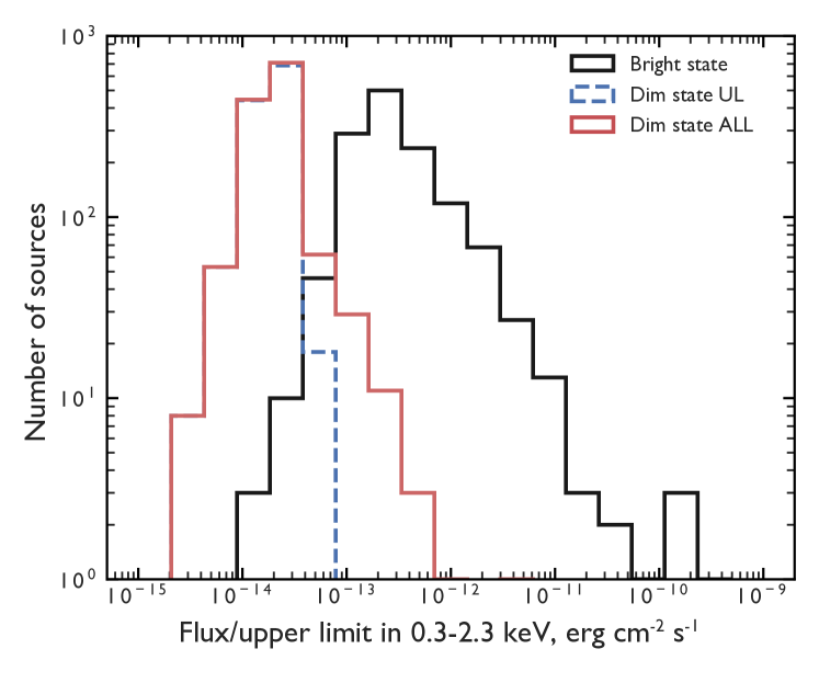
Figure 1: Flux distribution of the sample of highly variable sources in the 0.3–2.3 keV energy band. The black histogram indicates the maximum fluxes recorded for each source among the five SRG/eROSITA surveys. The red histogram indicates the minimum recorded fluxes for each source or the upper flux limits (also indicated separately by the dashed line) if the source was not detected with a likelihood exceeding the threshold value of 6 in the survey relative to which the most significant change in the flux in the bright state was obtained.

3.1 X-ray Light Curves

To construct the light curves of eROSITA X-ray sources, we used the method of forced PSF photometry. We performed forced PSF photometry based on data from each of the individual six-month sky surveys, with the positions and extents of the sources having been fixed at the values found from the sum of all surveys. Thus, the refitting procedure was used only to estimate the flux $F_{i}$ in the $i$-th sky survey and the 68% lower and upper limits on this flux, $F^{l}_{i}$ and $F^{u}_{i}$, respectively. Note that the total number of sources was fixed according to the combined catalog, and no filtering by detection significance was performed at the stage of forced photometry. At the same time, the lower flux limit for some sources could be zero.

3.2 Selection Method

To determine the confidence level of source flux change between surveys, we assumed that the measured flux from the source was a random variable $f_{i}$ with a normal probability density distribution and a mean $F_{i}$. The standard deviation $\sigma_{i}$ of the normal distribution was approximated by the mean error in the flux for the sources whose lower flux limit was above zero: $\sigma_{i}=(F^{u}_{i}-F^{l}_{i})/2$. Since the lower flux limit in the optimization procedure of the maximum likelihood method was set equal to zero, the flux probability distribution for faint sources with $F_{i}\sim\sigma_{i}$ becomes asymmetric and deviates significantly from the normal distribution. In this paper we neglected these deviations using only the upper flux limit to calculate the standard deviation for the faintest sources: $\sigma_{i}=F^{u}_{i}-F_{i}$. This leads to some underestimation of the statistical detection significance of the flux variability relative to the surveys with low fluxes obtained by the method of forced photometry, but does not affect significantly the selection of sources with $F_{i}>3\sigma_{i}$, which will mostly be discussed in this paper. In our future publication devoted to the full catalog of highly variable AGNs, including sources with $F_{i}<3\sigma_{i}$ in any of the surveys, we will take into account a realistic flux probability distribution for situations with low fluxes.

Assuming that the measurements of the flux from a source in surveys $i$ and $j$ are completely independent, the probability distribution of their ratio, $r=f_{i}/f_{j}$, can be written as follows:

$$p_{r}(r)=\int_{-\infty}^{+\infty}|f_{j}|p_{f,i}(rf_{j})p_{f,j}(f_{j})df_{j}$$ (1)

Using the normal approximation for the flux distribution $p_{f,i}=N(F_{i},\sigma_{i})$ will have the following form (see, e.g., Hinkley, 1969):

$$p_{r}=\frac{b(r)\cdot d(r)}{a^{3}(r)}\frac{1}{\sqrt{2\pi}\sigma_{i}\sigma_{j}}\left[\Phi\left(\frac{b(r)}{a(r)}\right)-\Phi\left(-\frac{b(r)}{a(r)}\right)\right]\\ +\frac{1}{a^{2}(r)\cdot\pi\sigma_{i}\sigma_{j}}e^{-\frac{c}{2}},$$ (2)

where

$$a(r) =\sqrt{\frac{1}{\sigma_{i}^{2}}r^{2}+\frac{1}{\sigma_{j}^{2}}}$$

$$b(r) =\frac{F_{i}}{\sigma_{i}^{2}}r+\frac{F_{j}}{\sigma_{j}^{2}}$$

$$c =\frac{F_{i}^{2}}{\sigma_{i}^{2}}+\frac{F_{j}^{2}}{\sigma_{j}^{2}}$$

$$d(r) =e^{\frac{b^{2}(r)-ca^{2}(r)}{2a^{2}(r)}}$$

and $\Phi$ is the cumulative normal distribution function

$$\Phi(x)=\int_{-\infty}^{x}\,\frac{1}{\sqrt{2\pi}}e^{-\frac{1}{2}y^{2}}\ dy\,.$$ (3)

For each source from the combined catalog and for each pair of surveys, using Eq. 2, we calculated the cumulative probability that the flux ratio $r=f_{i}/f_{j}>0.1$ provided that in the $j$-th survey the source was brighter than in the $i$-th survey, i.e., $F_{j}>F_{i}$. In other words, we calculated the probability that the true flux from the source in the two surveys changed by less than a factor of 10. This probability was calculated for all of the possible combinations of our five surveys. The source passed the selection criterion and was included in our sample of highly variable sources if the probability described above was less than $2.7\cdot 10^{-3}$ at least for one pair of surveys. Note that as the probability threshold we arbitrarily chose the value corresponding to the $3\sigma$ confidence level for a Gaussian distribution. Taking into account the fact that the number of trials (i.e., the number of all possible pairs of surveys) is 10, we expect that in the final catalog of highly variable AGNs there will be a few percent of the objects whose true variability amplitude is slightly less than 10.

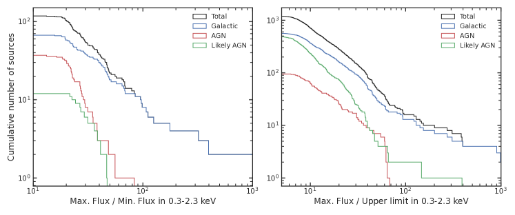
Figure 2: Distribution of the sample of highly variable sources in maximum variability amplitude $R_{X}$ recorded based on the five SRG/eROSITA surveys in the 0.3–2.3 keV energy band. The left panel shows the sources that are detected in the surveys in which their lowest flux was recorded (likelihood $\geq 6$). In this case, $R_{X}$ is defined as the ratio of the maximum flux to the minimum one among all surveys. The right panel shows the sources that are not detected in the surveys relative to which the most significant change in the flux was obtained. For these sources $R_{X}$ is defined as the ratio of the maximum flux to the $3\sigma$ upper flux limit. The black, blue, red, and green lines indicate the cumulative histogram, respectively, for all sources, the sources classified as Galactic ones, the spectroscopically confirmed AGNs, and the AGN candidates selected from the remaining sources (Subsection 3.4). For some of the sources shown on the right panel $R_{X}<10$, which is a consequence of the method of calculating the lower limit to calculate $R_{X}$ using the $3\sigma$ flux limit in the low state.

Table 1: The list of highly variable AGNs detected in the low state

No.	eROSITA source	$F^{max}_{0.3-2.3}$	$R_{X}$	Name	Spec. class	z	Reference
		erg s-1 cm-2
1	SRGE J143359.2+400636	$1.3\times 10^{-11}$	83.3	PGC 2160796	AGN-2	0.099	DR16
2	SRGE J010415.8+402244	$2.1\times 10^{-12}$	55.6	LAMOSTJ010415.77+402243.9	AGN-1	0.193	LAMOST
3	SRGE J061310.2+502628	$3.9\times 10^{-12}$	48.4	NPM 1G+50.0043	AGN-1	0.019	2MAGN
4	SRGE J122057.8+813600	$9.1\times 10^{-13}$	47.2
5	SRGE J134954.6+432857	$2.5\times 10^{-12}$	46.4	LEDA 2221805		0.045	SDSS-IV
6	SRGE J164147.7+700806	$6.8\times 10^{-13}$	41.0	NPM 1G+70.0164			MQ
7	SRGE J161630.7+354230	$2.2\times 10^{-12}$	38.4	NGC 6104	AGN-1	0.028	LOZAGN
8	SRGE J025436.4+152545	$1.3\times 10^{-12}$	38.4	PGC 1484380			CMO
9	SRGE J004730.3+154149	$1.9\times 10^{-12}$	38.1	MCG+02-03-002	LINER	0.031	DR16
10	SRGE J091935.9+753945	$1.6\times 10^{-12}$	35.8	GAIA 1124646674042078464		(0.5)	GAIA3
11	SRGE J024519.6-025627	$1.5\times 10^{-12}$	35.0	SDSS J024519.63-025628.1	BLLac		DR16
12	SRGE J163323.5+471900	$7.9\times 10^{-13}$	34.8	IRAS 16319+4725	AGN-1	0.116	LOZAGN
13	SRGE J174036.5+534624	$7.1\times 10^{-13}$	31.2	87GB 173932.3+534742	BLLac		4LAC
14	SRGE J073203.1+680336	$9.4\times 10^{-13}$	31.2				Palomar
15	SRGE J130600.3+330325	$1.2\times 10^{-12}$	29.6	PGC 2022001	AGN-1	0.088	DR16Q
16	SRGE J150311.8+111026	$1.5\times 10^{-12}$	29.3	SDSS J150311.67+111027.3	AGN-1	0.043	LOZAGN
17	SRGE J213946.2+113817	$3.1\times 10^{-12}$	29.1
18	SRGE J160752.0+444125	$1.4\times 10^{-12}$	28.6	LAMOSTJ160751.95+444124.6	AGN-1	0.718	LAMQ5
19	SRGE J135255.7+252900	$1.1\times 10^{-12}$	27.8	KUG 1350+257	AGN-1	0.064	LOZAGN
20	SRGE J011739.4-025626	$1.5\times 10^{-12}$	27.5	GJ0117394-025627	AGN-2	0.051	6dAGN
21	SRGE J175340.2+555128	$5.1\times 10^{-13}$	27.0	LEDA 2516819
22	SRGE J215717.0-263100	$1.6\times 10^{-12}$	26.9	2MASX J21571697-2630596	AGN-2	0.034	6dF
23	SRGE J145933.2+152742	$1.4\times 10^{-12}$	26.7	PGC 1485268	AGN-1	0.074	LOZAGN
24	SRGE J000415.2+173454	$1.7\times 10^{-12}$	26.5				Palomar
25	SRGE J155926.1+521237	$9.7\times 10^{-13}$	26.5	SDSS J155926.11+521235.2	AGN-2	0.042	LOZAGN
26	SRGE J142408.5+210520	$9.4\times 10^{-13}$	26.4	PGC 1642489	AGN-1	0.047	LOZAGN
27	SRGE J010812.6-114403	$3.4\times 10^{-12}$	24.1	IRAS 01056-12009			Palomar
28	SRGE J135321.5+373055	$1.3\times 10^{-12}$	23.8	PGC 2102603	AGN-1	0.107	LOZAGN
29	SRGE J150809.2+130031	$1.1\times 10^{-12}$	23.2	SDSS J150809.20+130032.4	AGN-1	0.086	LOZAGN
30	SRGE J155344.3+122233	$1.6\times 10^{-12}$	22.7	2MASX J15534435+1222337	LINER	0.035	DR16
31	SRGE J153552.5+143104	$2.7\times 10^{-12}$	22.7	AKN 479	AGN-2	0.020	LOZAGN
32	SRGE J124339.2+700515	$1.9\times 10^{-12}$	22.5	WISEA J124339.43+700517.0			MQ
33	SRGE J162012.8+400907	$5.3\times 10^{-12}$	22.4	KUG 1618+402	AGN-1	0.028	LOZAGN
34	SRGE J142607.6+340425	$1.2\times 10^{-12}$	22.3	CSO 450	BLLac	1.553	FIRST
35	SRGE J012633.6+313658	$2.3\times 10^{-12}$	22.1	MCG 5-04-059	AGN-1	0.045	Osterbrock
36	SRGE J152410.3+485409	$8.6\times 10^{-13}$	22.0	SDSS J152410.34+485409.7	AGN-1	0.145	LOZAGN
37	SRGE J121755.1+583936	$1.8\times 10^{-12}$	21.8	CGCG 293-9	AGN-1	0.023	LOZAGN
38	SRGE J163016.2+584247	$1.4\times 10^{-12}$	21.5	NPM 1G+58.0189
39	SRGE J035309.6+565431	$2.1\times 10^{-12}$	21.5	GB6 J0353+5654	BLLac		4LAC
40	SRGE J155829.3+271714	$2.3\times 10^{-12}$	20.9	PGC 1803429	AGN-1	0.090	LOZAGN
41	SRGE J142352.1+245417	$1.5\times 10^{-12}$	20.8	SDSS J142352.08+245417.1	AGN-2	0.074	DR16
42	SRGE J142812.0+511115	$1.2\times 10^{-12}$	20.2	SDSS J142811.88+511116.6	AGN-1	0.129	LOZAGN
43	SRGE J160855.5+155200	$2.7\times 10^{-12}$	20.0	SDSS J160855.60+155200.2	AGN-1	0.115	DR16Q
44	SRGE J130020.0+613919	$2.6\times 10^{-12}$	19.8	MCG 10-19-011	AGN-1	0.052	LOZAGN
45	SRGE J131443.9+234826	$2.5\times 10^{-12}$	19.3	TXS 1312+240	BLLac	2.060	DR16Q
46	SRGE J181214.1+215305	$2.2\times 10^{-12}$	18.5	CGCG 142-19	AGN-2	0.018	Veron
47	SRGE J021749.0+014449	$2.6\times 10^{-12}$	18.4	PKS 0215+015	AGN-1	1.715	Boisse
48	SRGE J181335.1+314418	$8.6\times 10^{-12}$	16.3	B2 1811+31	BLLac	0.117	EXOSAT
49	SRGE J022239.6+430208	$1.1\times 10^{-11}$	13.1	3C 66A	BLLac	0.444	BZCAT

The eROSITA source name corresponds to the best X-ray coordinates; the maximum variability amplitude $R_{X}=F^{max}/F^{min}$ is defined as the ratio of the maximum flux to the minimum one from the source fluxes in the 0.3–2.3 keV energy band recorded among all surveys; $F^{max}_{0.3-2.2}$ is the highest X-ray flux from the source (without any correction for absorption); the spectral classes of the sources 0.3–2.2 keV and their redshifts ($z$) were determined in the papers specified in the “Reference” column, for a detailed description of the notation, see Section 4 in the text of the paper.

3.3 Sample

The sample of highly variable sources obtained in this way contains 1325 sources. Fig. 1 shows the flux distribution for our sample of sources in the 0.3–2.3 keV energy band. The black histogram indicates the fluxes found by the method of forced photometry in the surveys in which the maximum flux was recorded (these times will be called the source bright state). The red histogram indicates the source fluxes or the upper flux limits in the surveys relative to which the most significant change in the flux was found (the source dim state). In this case, if the detection significance of a source in the dim state was below the detection likelihood threshold ($<6$), then as the source flux for the red histogram in Fig. 1 we used the 3-$\sigma$ upper limit obtained from the sensitivity maps of the eROSITA surveys (the contribution of such sources is indicated by the blue dashed histogram). Below in the paper, to parameterize the maximum variability amplitude detected from all of the sky surveys available for a given source, we will use the quantity $R_{X}$ defined as the ratio of the flux from the source in its bright state (black histogram) to the flux or the upper flux limit for the source in its dim state (red histogram).

3.4 Classification of the Selected Sources

Our sample of highly variable sources was cross-correlated with the Gaia eDR3 catalog (Gaia Collaboration et al., 2021) to determine the Galactic sources. We identified an X-ray source as a Galactic one if all of the sources from the Gaia catalog falling into its position error circle had significant parallax and/or proper motion measurements with S/N$\geq 5$. When determining the confidence level of the proper motion measurement, we checked both the proper motion components in equatorial coordinates and the total proper motion of the source. As the position error circle of the X-ray sources we used a 98% error circle; the typical radii of the position error circle for the selected eROSITA sources in the bright state are $\approx 5$". As a result of this procedure, we selected 630 candidates for highly variable Galactic sources.

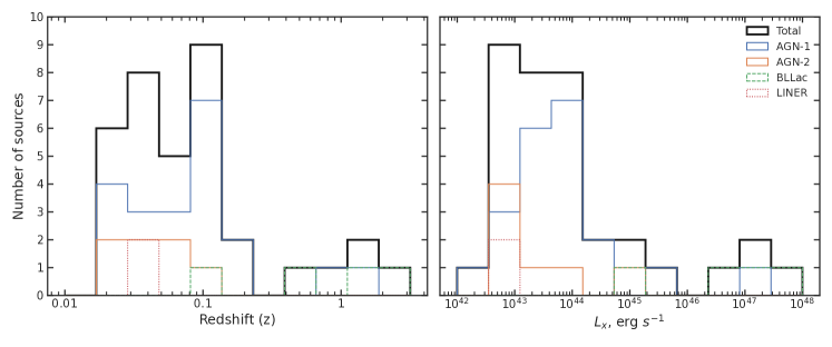
Figure 3: Left: histogram of the redshift distribution of the sources from Table 3.2. The black color indicates the combined distribution; the blue, orange, green, and red colors indicate the distributions of type 1 and 2 AGNs, BL Lac objects, and LINER galaxies, respectively. Right: the rest-frame X-ray luminosity distribution in the 0.3–10 keV energy band based on the eROSITA surveys during which the maximum X-ray flux from the sources was recorded (see Table LABEL:tab:params).

Fig. 2 shows the cumulative distribution of the sources in maximum variability amplitude ($R_{X}$). The left panel in Fig. 2 shows the sources for which the detection significance in the dim state (i.e., in the survey relative to which the most significant change in the flux was recorded) was above the detection likelihood threshold ($\geq 6$). The total number of such sources was 118; we identified 67 of them as Galactic sources. In the remaining sample of 51 sources two more sources were excluded from our further analysis as candidates for tidal disruption events (TDEs) based on the spectroscopic data obtained by the SRG/eROSITA ground support group.

The right panel in Fig. 2 shows the distribution for all of the remaining sources from our sample (1207 sources), 563 of which were identified as Galactic sources. In this case, the lower limit on the maximum variability amplitude that was calculated relative to the $3\sigma$ upper limit found from the sensitivity maps is shown. Note that for some of the sources shown on the right panel the variability amplitude $R_{X}<10$. This is a consequence of the method for calculating the lower limit on $R_{X}$ using the $3\sigma$ upper flux limit in the low state.

Our further classification of the candidates for extragalactic sources included their cross-correlation with the Million Quasars (Milliquas, v7.7, Flesch, 2021, 2015) catalog. The intersections of eROSITA X-ray sources with sources from the Milliquas catalog and having spectroscopically confirmed classes of objects and redshifts fell into the AGN group indicated on the right and left panels in Fig. 2 by the red solid lines. There were a total of 132 such sources (37 and 95 on the left and right panels, respectively). From the remaining group of unidentified sources we excluded the confirmed TDEs (from the published samples by Sazonov et al. 2021 and Khorunzhev et al. and from the lists of confirmed TDEs that will be published in succeeding papers) and the known classified transient events associated with supernova explosions and GRB afterglows based on Zwicky Transient Facility (ZTF; Bellm et al. 2019; Graham et al. 2019; Masci et al. 2019) and Asteroid Terrestrial-impact Last Alert System (ATLAS; Tonry et al. 2018; Smith et al. 2020) data. Thus, we excluded 60 more sources. The sources remaining unclassified after all of the described procedures (12 and 496 on the left and right panels, respectively) were assigned to the group of AGN candidates; they are indicated in Fig. 2 by the green line. Note that some of the unidentified candidates for extragalactic sources have signatures pointing to the AGN nature, such as the color $W_{1}-W_{2}>0.8$ (Assef et al., 2013) in the WISE infrared all-sky survey (Wright et al., 2010). Four sources from the AGN candidates on the left panel in Fig. 2 can be classified by this criterion as AGNs, while another 125 sources among the AGN candidates on the right panel have such a color.

In this paper we do not consider the completeness of our sample of highly variable AGNs and AGN candidates; it will be studied in more detail and described in the next paper of our series. The goal of this paper is to present a small group of the brightest and reliably selected highly variable AGNs (and AGN candidates), each of which is of scientific interest in its own right. Note, however, that the identification algorithm described above uses a 98% radius of the position error circle for X-ray sources (the position errors of optical sources are negligible), which makes a corresponding contribution to the completeness and purity of the sample being obtained, $\sim 2$%. Note that this contribution is not decisive. Besides, the 55 AGN candidates indicated by the green line on the right panel in Fig. 2 have a mixed composition of Gaia counterparts in the X-ray position error circle; at least some of them may turn out to be Galactic sources.

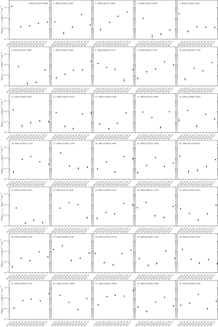
Figure 4: Long-term SRG/eROSITA X-ray light curves in the 0.3–2.3 keV energy band for the sample of highly variable AGNs given in Table 3.2. Each data point corresponds to the survey-averaged flux.

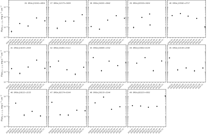
Figure 4: Continued.

4 Highly variable AGNs detected in their low state

The subsequent part of the paper is devoted to investigating the subsample of highly variable AGNs and their candidates for which the low-state flux was measured with a likelihood $\geq 6$, roughly corresponding to a confidence level of $\approx 3\sigma$ for a Gaussian dis- tribution. For these objects we can calculate the variability parameter $R_{X}$ with a sufficient accuracy and in many cases investigate their spectral characteristics in the low state.

4.1 Optical Classification and Redshifts

The list of these objects and their basic parameters are given in Table 3.2. Of the 49 objects, 37 are spectroscopically confirmed AGNs, for 35 of which the redshifts were also measured, and the other 12 sources were classified by us as AGN candidates. The RX distribution of this sample has already been discussed above and corresponds to the solid red and green lines on the left panel in Fig. 2. The information specified in the “name”, “spectral class”, and “z” (redshift) columns of the Table 3.2 is given in accordance with the previously published papers specified in the separate “reference” column. The following notation is used: DR16 — SDSS-DR16 (Ahumada et al., 2020), DR16Q — SDSS-DR16Q (Lyke et al., 2020), LAMOST — LAMOST Pilot Surveys (Huo et al., 2013), 2MAGN — 2MASS AGN (Zaw et al., 2019), SDSS-IV — SDSS-IV MaNGA Sample (Wake et al., 2017), LOZAGN — Low-redshift AGN (Liu et al., 2019), GAIA3 — Gaia DR3 QSO candidates (Gaia Collaboration et al., 2022), 4LAC — Fermi AGN v4 DR3 (The Fermi-LAT collaboration et al., 2022a), LAMQ5 — LAMOST QUASAR DR5/DR4 (Yao et al., 2019), 6dF — 6dF galaxy survey (Jones et al., 2009), 6dAGN — 6dF AGN, MQ — Milliquas (Flesch, 2021, 2015), FIRST — FIRST Bright Quasar Survey (White et al., 2000), Osterbrock (Osterbrock, 1977), 4LAC — Fermi AGN v4 DR3 (The Fermi-LAT collaboration et al., 2022b), Veron (Veron et al., 1997), Boisse (Boisse & Bergeron, 1988), EXOSAT — EXOSAT High Galactic Latitude Survey (Giommi et al., 1991), BZCAT — Roma-BZCAT (Massaro et al., 2009).

For three sources from Table 3.2 the SRG/eROSITA ground support group in collaboration with scientists from the California Institute of Technology obtained optical spectra at the Palomar Observatory (marked as “Palomar” in Table 3.2); one more source from the table was imaged with the Russian telescope at the Caucasus Mountain Observatory (CMO) of the Sternberg Astronomical Institute of the Moscow State University. The optical data on these sources will be published in a separate paper.

Among the presented sample 21 sources are spectroscopically confirmed type 1 AGNs (43%), 7 sources are type 2 AGNs (14%), another 7 are blazars (14%), and 2 are LINER AGNs (4%). The remaining 12 sources have no optical classification from the published papers to date (24%).

4.2 X-ray Light Curves

Fig. 4 shows the eROSITA X-ray light curves in the 0.3–2.3 keV energy band for the sample of sources from Table 3.2. Each light curve includes four or five flux measurements by the method of forced PSF photometry. The time interval between adjacent measurements is six months.

The light curves shown in Fig. 4 are characterized by a large amplitude of flux variations, in complete agreement with the source selection criterion. They exhibit a great variety in variability pattern, but their classification is complicated and, probably, will not be quite reliable and unambiguous due to the small number of measurements, 4 or 5. In some cases, astrophysically motivated classification and interpretation of the X-ray light curves can be made using spectral and (quasi-) simultaneous multiwavelength information, which our succeeding papers will be devoted to. One of the obvious questions that X-ray spectroscopy will help to answer is whether the abrupt or short-term (on time scales $\sim 6$ months) drop in the flux is associated with an increased absorption. In particular, in Section 5 we will identify the class of faded sources and discuss their spectral properties.

$N_{H,gal}$ is the Galactic absorption toward the source from the HI4PI maps (HI4PI Collaboration et al., 2016); $N_{H}$ and $\Gamma$ are, respectively, the absorption parameter and the photon index for the best-fit power-law spectral model in the 0.3–8 keV energy band; $L_{X}$ is the rest-frame X-ray luminosity corrected for Galactic absorption in the 0.3–10 keV energy band. The characteristics of the spectra are based on the SRG/eROSITA survey in which the maximum flux from the source was recorded; gof (goodness-of-fit) is the probability that the observed deviation of the data from the model is the result of random fluctuations. The model with $p$-value $<2.7\cdot 10^{-3}$ can be rejected by the data at a $3\sigma$ confidence level. The errors correspond to a 90% confidence level.

4.3 X-ray Spectra

The criterion for selecting the sample of sources presented in Table 3.2 allows the characteristics of their spectra to be determined not only for the surveys where the maximum flux was recorded, but also in the state with the minimum flux, although the number of such spectra is often not enough for the parameters of the spectral model to be reliably constrained. The source spectra were analyzed for each survey separately in the 0.3–8 keV energy band.

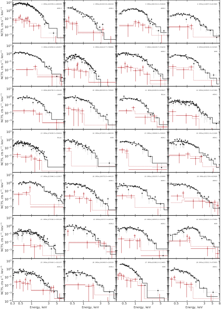
Figure 5: The X-ray spectra of objects from the sample of highly variable AGNs obtained by eROSITA during the SRG sky surveys in which the maximum (black dots with error bars) and minimum (red dots) fluxes from the source were recorded. The solid line indicates the best-fit power-law spectral models with absorption. The parameters of the models for the high state are given in Table LABEL:tab:params. The spectral channels were binned with a significance of at least $1\sigma$ (only for illustration).

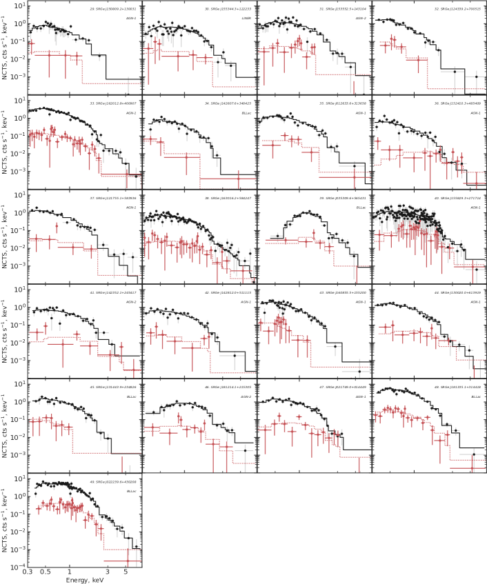
Figure 5: Continued.

As the basic spectral model we used a power law with absorption: tbabs*cflux*pow in the XSPEC notation. The absorption parameter $N_{\rm H}$ was determined when fitting the spectral model for the spectra with at least 50 counts in the energy band under consideration; in other cases, the parameter was fixed at the values equal to the Galactic absorption toward the sources based on the HI4PI maps (HI4PI Collaboration et al., 2016). The elemental abundances in the absorption model were specified in accordance with Wilms et al. (2000). The parameters for our best-fit models for the bright state of the sources are given in Table LABEL:tab:params. In the bright state for all sources $N_{\rm H}$ was determined from the data (all spectra have $>50$ counts). The spectra of the sources in the bright and dim states, along with the corresponding best-fit power-law models, are shown in Fig. 5. Note that the spectra of some sources in the bright state are poorly described by the power-law model. In particular, as follows from the derived goodness-of-fit values, the power-law model with absorption can be rejected at a confidence level $>3\sigma$ for the sources SRGE J1433+4006 (source no. 1 in Table LABEL:tab:params), SRGE J0104+4022 (no. 2), and SRGE J1641+7008 (no.6). The goal of using the power-law model here is a homogeneous characterization of the spectral hardness of the objects from the presented sample. Note also that within the power-law model the absorption parameter in many cases exceeds noticeably the expected Galactic absorption, at a confidence level $\geq 90\%$ for 15 sources.

Using the fitting results for the cflux model component, we calculated the rest-frame X-ray luminosities of the sources in the 0.3–10 keV energy band corrected for the absorption in the Galactic interstellar medium. The following cosmological parameters were used to calculate the luminosities: $H_{0}=70$ km s^-1 and $\Omega_{M}=0.3$. Table LABEL:tab:params gives the luminosities only for the sources with spectroscopically measured redshifts. Fig. 3 shows the distribution of the sample of sources from Table 3.2 in redshift (left panel) and X-ray luminosity (right panel) for the bright states. The redshifts and X-ray luminosities of the presented sample of sources lie in the ranges $z=0.018$–$2.06$ and $L_{X}=3\cdot 10^{42}$–$3\cdot 10^{47}$ erg s^-1, respectively.

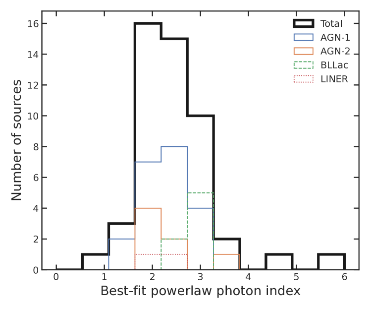
Figure 6: Distribution of the sources in photon index for the power-law spectral model with absorption in the states with the maximum flux (see Table LABEL:tab:params). The black color indicates the combined distribution; the blue, orange, green, and red colors indicate the distributions of type 1 and 2 AGNs, BL Lac objects, and LINER galaxies, respectively (see Table 3.2).

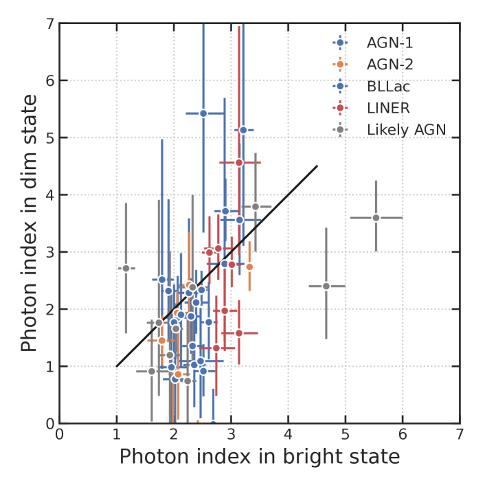
Figure 7: Comparison of the photon indices of the power-law model for the objects from Table 3.2 in the states with the minimum (vertical axis) and maximum (horizontal axis) fluxes. The $1\sigma$ errors. Only the objects for which the sum of the upper and lower measurement errors of the photon index in the low state does not exceed 4 are shown.

Fig. 6 shows the distribution of the sources in photon index for the bright-state spectra. The median of the distribution corresponds to a photon index of 2.3, while 68% of the sample have photon indices in the range from 2 to 3. We can note three sources that lie well outside this distribution: SRGE J1641+7008 (no. 6) and SRGE J0108-1144 (no. 27) with photon indices of $4.63_{-0.46}^{+0.60}$ and $5.48_{-0.68}^{+0.83}$, respectively, SRGE J2139+1138 (no. 17) with a photon index of $1.2\pm 0.1$. Below we will consider their spectra in more detail.

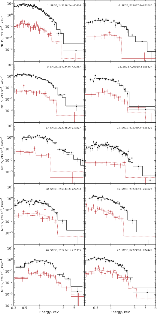
Figure 8: The X-ray spectra of the faded AGNs in the second survey. The black color indicates the high-state spectra (the first survey); the red color indicates the combined low-state spectra (surveys 2–5). The spectral channels were binned with a significance of at least $2\sigma$ (only for illustration).

Fig. 7 compares the derived photon indices of the sources during their bright and dim states. An asymmetry in the distribution of data points is clearly seen: the high-state spectra are, on average, softer than the low-state ones. Indeed, comparing the a posterior probability distribution for the parameter $\Gamma$ from the spectrum during the survey with the maximum flux from the source with the distribution from the survey with the minimum flux, we detected nine sources for which an increase in the photon index in the bright state is observed at a confidence level $>90\%$, namely sources no. 3, 6, 20, 22, 27, 36, 39, 44, and 47. The most significant ($>3\sigma$) change in the photon index was found for the sources SRGE J1524+4854 (no. 36) and SRGE J1300+6139 (no. 44). The following low-state model parameters were obtained for them: $\Gamma=-0.05_{-0.91}^{+1.11}$ and $\Gamma=0.87_{-0.67}^{+0.84}$. For the same confidence level (90%) we detected no source from our sample for which a statistically significant decrease in the photon index in the bright state would be observed (but two such cases were detected among the faded AGNs when adding the data of several surveys in the low state, see the next section).

5 Discussion of individual sources

In this section we discuss the most interesting sources from the catalog in Table 3.2.

5.1 Fading AGNs

Based on the pattern of the light curves shown in Fig. 4, among them we can identify the group of faded sources for which a significant drop in the X-ray flux was recorded between two surveys, whereupon in the succeeding surveys the flux was not restored to values comparable to the maximum one. Such variability can be the result of a source outburst or, alternatively, a longer transition from the high to low state. As has already been noted above, this separation is arbitrary, since, interpreting 4 or 5 flux measurements, we cannot rule out a more complex picture of variability on long time scales. Nevertheless, it is of interest to compare the X-ray spectra of such sources in the high and low states. For this purpose, without claiming to be complete, we identified ten sources using the following selection criteria: (i) the source flux decreased in the second survey relative to the first one by more than a factor of 8 and (ii) in all of the subsequent observations it remained no more than 20% of the flux in the first survey. To improve the statistical quality of the low- state spectra, we combined the data from all of the surveys in which the source was in the low state. The high- and low-state spectra obtained in this way are presented in Fig. 8, while the best-fit photon indices in the high and low states are presented in Fig. 9.

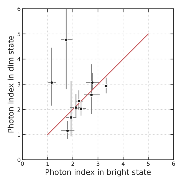
Figure 9: Comparison of the photon indices of the power-law model for the sample of faded AGNs. The photon index for the spectra of the sources in the first survey (bright state) and for the spectra from the sum of surveys 2–5 (dim state) is shown along the horizontal and vertical axes, respectively. The errors are given at a 68% confidence level.

As follows from Fig. 8, the dramatic drops in the source luminosity, as a rule, are not accompanied by significant spectral changes. Thus, we immediately rule out the great absorption variations as a cause of the flux changes (in the sources under consideration). Two sources exhibited a change in the spectral shape of moderate statistical significance: SRGE J1220+8136 (no. 4) and SRGE J2139+1138 (no. 17, Fig. 9). Interestingly, these two sources are characterized by the hardest high-state spectra (see Table LABEL:tab:params). In this sense they show a trend opposite to most of the sources under consideration (Fig. 7). We found an increase in the photon index in the power-law model with absorption in the low state for these two sources and an increase in the absorption column density $N_{H}$ at a confidence level $>90$% for the source SRGE J122057.8+813600 (according to the probability distributions of the parameters found from MCMC). The parameters of the power-law models in the low state for them are: $\Gamma=3.4_{-0.6}^{+4.0}$, $N_{H}=4.4_{-0.9}^{+8.8}\cdot 10^{21}$ cm^-2 for SRGE J122057.8+813600 and $\Gamma=2.4_{-0.2}^{+2.1}$, $N_{H}=1.0_{-0.2}^{+3.7}\cdot 10^{21}$ cm^-2 for SRGE J213946.2+113817 (the error corresponds to a 90% confidence level). For other faded sources we failed to detect statistically significant changes in their spectral parameters (see Fig. 9).

5.2 Sources with Anomalously Soft Spectra

Other interesting objects in Table 3.2 are the sources SRGE J1641+7008 (no. 6) and SRGE J0108-1144 (no. 27) having the softest high-state spectra with photon indices $\Gamma\approx 4.6\pm 0.3$ and $\Gamma\approx 5.7\pm 0.5$, respectively (see Table LABEL:tab:params). We fitted the high-state spectra of these sources by the simplest accretion disk model (diskbb in XSPEC, more complex models are more difficult to apply due to the unknown redshifts of these sources) and obtained the following parameters: $T_{in}=0.21_{-0.03}^{+0.02}$, $n_{H}=0.68_{-0.28}^{+0.53}\times 10^{21}$ cm^-2 for SRGE J164147.7+700806 and $T_{in}=0.15_{-0.02}^{+0.01}$, $n_{H}<0.68\times 10^{21}$ cm^-2 for SRGE J010812.6-114403. Note that for the first source the thermal model describes the observed spectra significantly better: $\delta$c-stat$=-7.0$. For the second source no improvement in the quality of the fit was found: $\delta$c-stat$=-0.1$.

Both sources have no published spectral classifications and redshifts. The X-ray position of SRGE J1641+7008 is compatible with the galaxy LEDA 2734260, which is also the known radio source VLAJ164147.34+700806.1.

The softness of the high-state spectra could suggest that they are associated with TDEs (Sazonov et al. 2021). However, the observed light curves of these sources are atypical for TDEs. Note also that we detected no optical transients for these sources based on open ZTF data. These sources require a further study, in particular, in the optical range.

5.3 SRGE J035309.6+565431

The source SRGE J0353+5654 (no. 39) possesses the highest absorption among the objects of our sample based on the power-law model fit (see Table LABEL:tab:params). Its X-ray position is compatible with the known blazar GB6 J0353+5654, which belongs to the class of blazars with a high-frequency synchrotron peak (HSP). Its optical spectrum is featureless, the redshift is unknown (Álvarez Crespo et al., 2016). No optical transients were detected in the position error circle either.

The X-ray light curve of SRGE J0353+5654 (see Fig. 4) exhibits abrupt changes in the flux in all four surveys. The simple thermal models with absorption describe the spectrum slightly more poorly than does the absorbed power-law spectrum, $\delta$c-stat$=+11.6$ (bbodyrad) and $\delta$c-stat$=+5.6$ (diskbb), with the absorption parameter for these models being consistent with the Galactic value toward the source. We obtained the following parameters for the diskbb model: $T_{in}=0.67_{-0.13}^{+0.11}$ keV and $N_{H}=6.5_{-1.0}^{+1.7}\times 10^{21}$ cm^-2. However, the physical motivation for the application of thermal spectral models to the description of the spectra for blazars is not obvious.

6 Conclusions

Although the X-ray flux variability is an integral property of accretion and, in particular, accretion onto SMBHs in AGNs, dramatic, by more than an order of magnitude, changes in the AGN luminosity on a time scale $\sim 1$ year are very rare. Moreover, in the standard picture of accretion onto a SMBH (Shakura & Sunyaev, 1973) their existence is difficult to explain. In view of their rarity, such events have been poorly studied, in particular, there is no estimate of their frequency and there is no clear picture of their abundance among AGNs of various types. The SRG/eROSITA all-sky X-ray survey for the first time has provided an opportunity to systematically study such events, to estimate the frequency of their occurrence and the association with specific AGN classes.

This paper is the first in our series of works aimed at searching for and studying highly variable AGNs and quasars based on the SRG/eROSITA all-sky survey data. We described the method of searching for such objects in the eROSITA catalog of X-ray sources and the methods of selecting AGNs and their candidates and analyzed the primary statistical properties of our preliminary catalog of 1365 highly variable objects.

Of the 1365 highly variable objects, for 630 we confirmed their Galactic origin with sufficient reliability, for another 60 we confirmed their association with tidal disruption events, and 675 are AGNs or their candidates. Thus, taking into account the fact that more than a million sources in the eROSITA catalog are AGNs and quasars, the fraction of such highly variable objects among AGNs is less than $\la 7\cdot 10^{-4}$, confirming the above assertion about the extreme rarity of such events.

In this paper we presented our catalog and studied in detail 49 highly variable AGNs and their candidates for which a statistically significant flux is detected in their low state. Many of these objects have been well studied in the optical range. Our analysis of their eROSITA X-ray spectra and the optical classification at this stage has not revealed obvious trends and predominant associations with specific AGN types. However, we can conclude already now that they are not associated predominantly with blazars. It is also interesting to note that the high states of AGNs, on average, are characterized by softer X-ray spectra.

Our study of these unique objects will be continued in the succeeding papers of this series.

Acknowledgements

This work is based on observations with the eROSITA telescope on board the SRG observatory. The SRG observatory was built by Roskosmos in the interests of the Russian Academy of Sciences represented by its Space Research Institute (IKI) in the framework of the Russian Federal Space Program, with the participation of the Deutsches Zentrum für Luft- und Raumfahrt (DLR). The SRG/eROSITA X-ray telescope was built by a consortium of German Institutes led by MPE, and supported by DLR. The SRG spacecraft was designed, built, launched and is operated by the Lavochkin Association and its subcontractors. The science data are downlinked via the Deep Space Network Antennae in Bear Lakes, Ussurijsk, and Baykonur, funded by Roskosmos. The eROSITA data used in this work were processed using the eSASS software system developed by the German eROSITA consortium and proprietary data reduction and analysis software developed by the Russian eROSITA Consortium. This work was supported by RSF no. 21-12-00343.

References

- Ahumada et al. (2020) Ahumada R., et al., 2020, ApJS, 249, 3
- Anderson (1962) Anderson T. W., 1962, The Annals of Mathematical Statistics, 33, 1148
- Antonucci (1993) Antonucci R., 1993, ARA&A, 31, 473
- Arnaud (1996) Arnaud K. A., 1996, in Jacoby G. H., Barnes J., eds, Astronomical Society of the Pacific Conference Series Vol. 101, Astronomical Data Analysis Software and Systems V. p. 17
- Assef et al. (2013) Assef R. J., et al., 2013, ApJ, 772, 26
- Bellm et al. (2019) Bellm E. C., et al., 2019, PASP, 131, 018002
- Boisse & Bergeron (1988) Boisse P., Bergeron J., 1988, A&A, 192, 1
- Brunner et al. (2022) Brunner H., et al., 2022, A&A, 661, A1
- Cash (1979) Cash W., 1979, ApJ, 228, 939
- Cramér (1928) Cramér H., 1928, Scandinavian Actuarial Journal, 1928, 13
- Flesch (2015) Flesch E. W., 2015, PASA, 32, e010
- Flesch (2021) Flesch E. W., 2021, arXiv e-prints, p. arXiv:2105.12985
- Gaia Collaboration et al. (2021) Gaia Collaboration et al., 2021, A&A, 649, A1
- Gaia Collaboration et al. (2022) Gaia Collaboration et al., 2022, arXiv e-prints, p. arXiv:2206.05681
- Geweke (1992) Geweke J., 1992, Bayesian statistics, 4, 641
- Gibson & Brandt (2012) Gibson R. R., Brandt W., 2012, The Astrophysical Journal, 746, 54
- Giommi et al. (1991) Giommi P., et al., 1991, ApJ, 378, 77
- Goodman & Weare (2010) Goodman J., Weare J., 2010, Communications in Applied Mathematics and Computational Science, 5, 65
- Graham et al. (2019) Graham M. J., et al., 2019, PASP, 131, 078001
- HI4PI Collaboration et al. (2016) HI4PI Collaboration et al., 2016, A&A, 594, A116
- Hinkley (1969) Hinkley D. V., 1969, Biometrika, 56, 635
- Huo et al. (2013) Huo Z.-Y., et al., 2013, AJ, 145, 159
- Jones et al. (2009) Jones D. H., et al., 2009, MNRAS, 399, 683
- Lanzuisi et al. (2014) Lanzuisi G., et al., 2014, The Astrophysical Journal, 781, 105
- Lawrence et al. (1987) Lawrence A., Watson M. G., Pounds K. A., Elvis M., 1987, Nature, 325, 694
- Liu et al. (2019) Liu H.-Y., Liu W.-J., Dong X.-B., Zhou H., Wang T., Lu H., Yuan W., 2019, ApJS, 243, 21
- Lyke et al. (2020) Lyke B. W., et al., 2020, ApJS, 250, 8
- Markowitz & Edelson (2004) Markowitz A., Edelson R., 2004, ApJ, 617, 939
- Masci et al. (2019) Masci F. J., et al., 2019, PASP, 131, 018003
- Massaro et al. (2009) Massaro E., Giommi P., Leto C., Marchegiani P., Maselli A., Perri M., Piranomonte S., Sclavi S., 2009, A&A, 495, 691
- Matt et al. (2003) Matt G., Guainazzi M., Maiolino R., 2003, Monthly Notices of the Royal Astronomical Society, 342, 422
- McHardy & Czerny (1987) McHardy I., Czerny B., 1987, Nature, 325, 696
- Middei et al. (2017) Middei R., Vagnetti F., Bianchi S., La Franca F., Paolillo M., Ursini F., 2017, Astronomy & Astrophysics, 599, A82
- Osterbrock (1977) Osterbrock D. E., 1977, ApJ, 215, 733
- Pavlinsky et al. (2021) Pavlinsky M., et al., 2021, A&A, 650, A42
- Peterson (2001) Peterson B. M., 2001, in Aretxaga I., Kunth D., Mújica R., eds, Advanced Lectures on the Starburst-AGN. p. 3 (arXiv:astro-ph/0109495), doi:10.1142/9789812811318_0002
- Predehl et al. (2021) Predehl P., et al., 2021, A&A, 647, A1
- Puccetti et al. (2014) Puccetti S., et al., 2014, The Astrophysical Journal, 793, 26
- Ricci et al. (2016) Ricci C., et al., 2016, The Astrophysical Journal, 820, 5
- Ricci et al. (2020) Ricci C., et al., 2020, The Astrophysical Journal Letters, 898, L1
- Sazonov et al. (2021) Sazonov S., et al., 2021, MNRAS, 508, 3820
- Shakura & Sunyaev (1973) Shakura N. I., Sunyaev R. A., 1973, A&A, 24, 337
- Shakura & Sunyaev (1976) Shakura N. I., Sunyaev R. A., 1976, MNRAS, 175, 613
- Shemmer et al. (2014) Shemmer O., et al., 2014, ApJ, 783, 116
- Shemmer et al. (2017) Shemmer O., Brandt W. N., Paolillo M., Kaspi S., Vignali C., Lira P., Schneider D. P., 2017, The Astrophysical Journal, 848, 46
- Smith et al. (2020) Smith K. W., et al., 2020, PASP, 132, 085002
- Stern et al. (2018) Stern D., et al., 2018, ApJ, 864, 27
- Sunyaev et al. (2021) Sunyaev R., et al., 2021, A&A, 656, A132
- The Fermi-LAT collaboration et al. (2022a) The Fermi-LAT collaboration et al., 2022a, arXiv e-prints, p. arXiv:2209.12070
- The Fermi-LAT collaboration et al. (2022b) The Fermi-LAT collaboration et al., 2022b, arXiv e-prints, p. arXiv:2209.12070
- Timlin III et al. (2020) Timlin III J. D., Brandt W. N., Zhu S., Liu H., Luo B., Ni Q., 2020, Monthly Notices of the Royal Astronomical Society, 498, 4033
- Tonry et al. (2018) Tonry J. L., et al., 2018, PASP, 130, 064505
- Uttley et al. (2002) Uttley P., McHardy I. M., Papadakis I. E., 2002, Monthly Notices of the Royal Astronomical Society, 332, 231
- Vagnetti et al. (2011) Vagnetti F., Turriziani S., Trevese D., 2011, A&A, 536, A84
- Vagnetti et al. (2016) Vagnetti F., Middei R., Antonucci M., Paolillo M., Serafinelli R., 2016, Astronomy & Astrophysics, 593, A55
- Veron et al. (1997) Veron P., Goncalves A. C., Veron-Cetty M. P., 1997, A&A, 319, 52
- Wake et al. (2017) Wake D. A., et al., 2017, AJ, 154, 86
- White et al. (2000) White R. L., et al., 2000, The Astrophysical Journal Supplement Series, 126, 133
- Wilms et al. (2000) Wilms J., Allen A., McCray R., 2000, ApJ, 542, 914
- Wright et al. (2010) Wright E. L., et al., 2010, AJ, 140, 1868
- Yao et al. (2019) Yao S., et al., 2019, ApJS, 240, 6
- Zaw et al. (2019) Zaw I., Chen Y.-P., Farrar G. R., 2019, ApJ, 872, 134
- Álvarez Crespo et al. (2016) Álvarez Crespo N., et al., 2016, The Astronomical Journal, 151, 95