Closed form expressions for the Green’s function of a quantum graph – a scattering approach

Abstract.

In this work we present a three step procedure for generating a closed form expression of the Green’s function on both closed and open finite quantum graphs with general self-adjoint matching conditions. We first generalize and simplify the approach by Barra and Gaspard [Barra F and Gaspard P 2001, Phys. Rev. E 65, 016205] and then discuss the validity of the explicit expressions. For compact graphs, we show that the explicit expression is equivalent to the spectral decomposition as a sum over poles at the discrete energy eigenvalues with residues that contain projector kernel onto the corresponding eigenstate.
The derivation of the Green’s function is based on the scattering approach, in which stationary solutions are constructed by treating each vertex or subgraph as a scattering site described by a scattering matrix. The latter can then be given in a simple closed form from which the Green’s function is derived.
The relevant scattering matrices contain inverse operators which are not well defined for wave numbers at which bound states in the continuum exists. It is shown that the singularities in the scattering matrix related to these bound states or perfect scars can be regularised. Green’s functions or scattering matrices can then be expressed as a sum of a regular and a singular part where the singular part contains the projection kernel onto the perfect scar.

Keywords: Quantum Graphs, Green’s functions, Wave scattering.

1. Introduction

Quantum graphs as metric graphs endowed with a Schrödinger operator and related similar models have a long history in mathematics, physics and theoretical chemistry [1, 2, 3, 4, 5, 6, 7]. Due to the simplicity of the model and the richness of properties and effects it can represent, quantum graphs have grown into an important tool in physics and mathematics. In spectral theory, they allow for a rigorous treatment of topics that are usually related to the study of (self- adjoint) partial differential operators, see [8] for an introduction and overview. The scattering approach to quantum graphs was introduced in 1997 by Kottos and Smilansky [9] and led to a wide range of applications in quantum chaos, see [10] for an overview. In this approach, the graph vertices are treated as scattering sites from which stationary solutions (energy eigenstates) are constructed. This approach has also been used for many physical applications beyond quantum chaos, including meta-material design [11], modelling the vibrations of coupled plates [12], as well as in formulating quantum random walks [13, 14] and quantum search algorithms [15]. One advantage of the scattering approach is that eigenvalue conditions can be written in terms of a secular equation involving the determinant of a unitary matrix of finite dimension $N$, where $N$ typically equals twice the number of edges on the graph. Similarly, the scattering matrix of an open quantum graph can be given in terms of a closed form expression involving finite dimensional matrices of size $N$ [16, 17].

In 2001, Barra and Gaspard [17] used the scattering approach to express the Green’s function of a quantum graph as a sum over trajectories in the spirit of semiclassical quantum mechanics. At the time, it was not yet clear within the physics community what scattering matrices are connected to matching conditions related to a well-defined self-adjoint Schrödinger operator on the metric graph. We generalize and simplify the approach [17] by using a simple three step procedure that leads to the Green’s function for general self-adjoint matching conditions for closed and open graphs with a finite number of edges. This directly provides a number of closed form expressions that, to the best of our knowledge, have not been given before (though implied in [17], see also [18], where closed form expressions are given for a few simple examples). These closed forms are of great practical advantage when dealing with explicit graphs as they sum all relevant trajectories. Moreover, they are the starting point of an analysis of the validity and convergence of Green’s function when expressed as a sum over trajectories. We thus hope to provide a more straightforward way of computing Green’s functions on graphs. This could lead to helpful insight into the growing literature on applications for Green’s functions on graphs that often require relatively cumbersome sums over trajectories, see [19, 20, 21] and references therein.

We also discuss in some detail cases where the sum over trajectories fails to converge while closed form expressions may be regularized. Indeed, when evaluating the scattering matrix on open graphs, such as those used in the construction of the Green’s function, one must take great care at frequencies corresponding to bound states in the continuum. These states vanish necessarily on the scattering leads and potentially lead to singular behaviour when considering the Green’s function. Scarring of eigenfunctions is a well-known semiclassical phenomenon in more general systems [22]. It has been known since the work of Schanz and Kottos [23] that quantum graphs allow for a much stronger scarring mechanism than in more general wave systems. These so-called perfect scars are non-vanishing only on a finite subset of the edges and vanish exactly in the remainder of the graph. They are easily constructed, for example, in certain quantum graphs with standard (Neumann- Kirchhoff) vertex matching conditions. For open graphs, bound states in the continuum are an example of perfect scars. Perfect scars lead to singularities in some inverted matrices that are used in the construction of scattering matrices and Green’s function and this implies non-convergence of the related sums over trajectories at the corresponding wave number. We will explain that both the scattering matrix and the Green’s function (outside the domain of the perfect scar) stay regular at these frequencies and give suitable regularised equations. These regularized expressions may be of practical importance even if there are no perfect scars on the graph. This is due to the far more generic phenomenon of almost perfect scars which was also described in [23]. These are states where the conditions for a perfect scar on a subgraph are fulfilled up to small terms leading to states which are only slightly coupled to outgoing channels. In the scattering matrix, almost perfect scars lead to what is known as topological resonances [24, 25]. In this context, a simplified variant of the regularization scheme we describe here has been used to derive the tails in the distribution of resonance widths [24].

The paper is structured as follows: In Sec. 2, the scattering representation is introduced for both closed and open quantum graphs. In Sec. 3, a three step procedure for generating a closed form expression for the Green’s function is introduced via the scattering approach. The expression is given generally for both closed and open quantum graph. It is assumed that the graph scattering matrix is non-singular and well defined. In Sec. 4, a formal definition is given for a scar state in terms of the quantum map. It is shown that the block component of the quantum map that refers to the compact portion of the graph is non-invertible. It is shown through a regularization of the scattering approach, that the full solution is indeed regular as it is evaluated within a reduced space. Further analysis of the scattering states for eigenenergies approaching a scar state are investigated D. In Sec. 5, we generate the scattered states and the corresponding Green’s function in the presence of scars for two examples, the open lasso, and the open star graph. We finally conclude this work in Sec. 6 with a brief summary and outlook.

2. The scattering approach for quantum graphs

To construct a quantum graph, we first consider a metric graph $\mathcal{G}(\mathcal{V},\mathcal{E},L)$. Here, $\mathcal{E}$ is the set of edges, $\mathcal{V}$ the set of vertices, and $L=\{\ell_{e}:e\in\mathcal{E}\}$ is the graph metric containing a set of edge lengths which are either real positive $\ell_{e}>0$ or infinite. The set of edges with finite length will be called the set of bonds $\mathcal{B}$ and the set of edges with infinite length will be called the set of leads $\mathcal{L}$. We consider two types of finite graphs:
i. Closed compact graphs where all edges are bonds and the number of edges $N_{\mathcal{E}}=|\mathcal{E}|$ is finite. Here, both ends of each edge are connected to a vertex.
ii. Open scattering graphs which consist of a compact graph with the addition of a finite set of leads. The leads are connected to a single vertex at one end. One may write the edge set as a union $\mathcal{E}=\mathcal{L}\cup\mathcal{B}$. With $N_{\mathcal{L}}=|\mathcal{L}|$ and $N_{\mathcal{B}}=|\mathcal{B}|$, one has $N_{\mathcal{E}}=N_{\mathcal{B}}+N_{\mathcal{L}}$.
For each bond $e\in\mathcal{B}$, we use a coordinate $x_{e}\in[0,\ell_{e}]$ with some (arbitrary but fixed) choice of direction. The coordinate defines a position on an edge such that $x_{e}=0$ and $x_{e}=\ell_{e}$ correspond to the vertices connected by the bond. For a lead $e\in\mathcal{L}$, coordinates $x_{e}\in[0,\infty)$ are defined such that $x_{e}=0$ corresponds to the vertex where the lead is attached. For each edge $e$, we refer to the directed edges as $e_{s}$ with $s=\pm$ indicating the direction in which $x_{e}$ increases ($s=+$) or decreases ($s=-$). A point on the graph is a pair $\mathbf{x}=(e,x_{e})$ of an edge and a coordinate.

The metric graph is turned into a quantum graph by adding a Schrödinger operator $\hat{H}$ which requires a set of boundary conditions on the graph vertices in order to become a self-adjoint problem. For this, we consider the Hilbert space $L^{2}(\mathcal{G})\equiv\bigoplus_{e\in E}L^{2}([0,\ell_{e}])$ of square integrable complex-valued functions $\boldsymbol{\Phi}(\mathbf{x})=\{\phi_{e}(x_{e})\}_{e\in\mathcal{E}}$ and define

(1) $$\left[\hat{H}\boldsymbol{\Phi}(\mathbf{x})\right]_{e}=-\frac{d^{2}}{dx_{e}^{2}}\phi_{e}(x_{e})+V_{e}(x_{e})\phi_{e}(x_{e})$$

with a potential $\boldsymbol{V}(\mathbf{x})=\{V_{e}(x_{e})\}_{e\in\mathcal{E}}$, that is, a real valued scalar function defined on $\mathcal{G}$. We will only consider free Schrödinger operators, that is, negative Laplacians, where $\boldsymbol{V}(\mathbf{x})=0$. To ensure that the second derivative is well defined and square integrable, one needs to restrict the domain of $\hat{H}$ to an appropriate Sobolev space. Apart from this standard restriction, the domain of $\hat{H}$ has to be further specified by appropriate boundary conditions at each vertex $v$ in order for $\hat{H}$ to define a self-adjoint operator. According to a theorem by Kostrykin and Schrader [26], the most general such boundary conditions at the vertex $v$ may be written in the form

(2) $$\sum_{\tilde{e}}\boldsymbol{A}_{e\tilde{e}}\phi_{\tilde{e}}(0)+\boldsymbol{B}_{e\tilde{e}}\frac{d\phi_{\tilde{e}}}{dx_{\tilde{e}}}(0)=0$$

for any $e$ connected to $v$ and the sum extends over edges $\tilde{e}$ connected to $v$. (We assumed here for simplicity that $x_{e}=0$ at the vertex for each edge $e$ connected to $v$.) The complex coefficients $\boldsymbol{A}_{e\tilde{e}}$ and $\boldsymbol{B}_{e\tilde{e}}$ refer to the elements $e\tilde{e}$ of two square matrices $\boldsymbol{A}$ and $\boldsymbol{B}$ of dimension $d_{v}$, the number of edges connected to $v$. In [26], it was proven that the matching conditions preserve self-adjointness if and only if two conditions are satisfied. First, the set of equations need to be independent which means that the rectangular $d_{v}\times 2d_{v}$ matrix $\left(\boldsymbol{A},\boldsymbol{B}\right)$, i.e. $\boldsymbol{A}$ and $\boldsymbol{B}$ being horizontally stacked, must have full rank $d_{v}$. Second, the product $\boldsymbol{AB}^{\dagger}=\boldsymbol{BA}^{\dagger}$ is a Hermitian matrix. The matrices $\boldsymbol{A}$ and $\boldsymbol{B}$ may be chosen independently for each vertex and we will often write $\boldsymbol{A}^{(v)}$ and $\boldsymbol{B}^{(v)}$ to indicate the vertex where these matrices act.

The self-adjointness of $\hat{H}$ implies a unitary evolution of the time-dependent Schrödinger equation $i\frac{d}{dt}\boldsymbol{\Phi}(t)=\hat{H}\boldsymbol{\Phi}(t)$. The stationary solutions $\boldsymbol{\Phi}(t)=e^{-iEt}\boldsymbol{\Psi}$ satisfy the (homogeneous) eigenproblem

(3) $$\left[\left(E-\hat{H}\right)\boldsymbol{\Psi}(\mathbf{x})\right]_{e}=\left(E+\frac{d^{2}}{dx_{e}^{2}}\right)\psi_{e}(x_{e})=0\ .$$

Here, $E$ is the energy. It implies furthermore that solutions to (3) only exist for real values of $E$ and the set of all such (generalized) eigenvalues forms the spectrum of $\hat{H}$. In the remainder we will only consider the positive part of their spectrum and write $E=k^{2}>0$ with the wave number $k>0$. In the following constructions, the energy appears as a variable that is not restricted to the spectrum.

Any solution to equation (3) fulfilling the prescribed boundary conditions at the vertices is expressed as a superposition of counter propagating plane waves, that is,

(4) $$\begin{split}\psi_{e}(x_{e})=&a^{\mathrm{in}}_{e_{-}}e^{-ikx_{e}}+a^{\mathrm{out}}_{e_{+}}e^{ikx_{e}}\\ =&a^{\mathrm{out}}_{e_{-}}e^{-ik(x_{e}-\ell_{e})}+a^{\mathrm{in}}_{e_{+}}e^{ik(x_{e}-\ell_{e})}\\ =&a^{\mathrm{in}}_{e_{-}}e^{-ikx_{e}}+a^{\mathrm{in}}_{e_{+}}e^{ik(x_{e}-\ell_{e})}\ .\end{split}$$

Here, $a^{\mathrm{in/out}}_{e_{\pm}}$ is the complex wave amplitude on edge $e$ propagating in the direction of increasing ($+$) or decreasing ($-$) $x_{e}$, heading $\mathrm{in}$ or $\mathrm{out}$ of a vertex. If $e$ is a lead only the amplitudes $a^{\mathrm{in/out}}_{e_{\pm}}$ at $x_{e}=0$ are used.
Introducing the $2N_{B}$-dimensional diagonal length matrix

(5) $$\mathbf{L}_{\tilde{e}_{\tilde{s}}e_{s}}=\delta_{e\tilde{e}}\delta_{s\tilde{s}}\ell_{e}$$

(where each edge length appears twice) the bond wave amplitudes can be mapped to one another by the diagonal square $2N_{B}$-dimensional matrix

(6) $$\mathbf{T}(k)=e^{ik\mathbf{L}}$$

that takes account of the phase difference between wave amplitudes across all bonds, that is,

(7) $$\mathbf{a}^{\mathrm{in}}_{\mathcal{B}}=\mathbf{T}(k)\ \mathbf{a}^{\mathrm{out}}_{\mathcal{B}}\ .$$

Here, $\mathbf{a}^{\mathrm{in/out}}_{\mathcal{B}}$ refers to the $2N_{\mathcal{B}}$ vector of plane wave coefficients on the directed bonds.
In addition, the graph wave amplitudes can be mapped onto one another across the vertices by taking account of the imposed vertex boundary conditions. For this one writes the matching conditions at a given vertex $v$ in the form of a $d_{v}\times d_{v}$ vertex scattering matrix $\boldsymbol{\Sigma}^{(v)}$, that is,

(8) $$\mathbf{a}^{(v),\mathrm{out}}=\boldsymbol{\Sigma}^{(v)}\mathbf{a}^{(v),\mathrm{in}}$$

where $\mathbf{a}^{(v),\mathrm{in/out}}$ are $d_{v}$ dimensional vectors that collect all incoming/outgoing amplitudes of plane waves on the edges $e$ in the neighborhood of vertex $v$. With the prescribed boundary conditions given in Eq. (2), $\boldsymbol{\Sigma}^{(v)}$ takes on the form

(9) $$\boldsymbol{\Sigma}^{(v)}(k)=-\left(\boldsymbol{A}^{(v)}+ik\boldsymbol{B}^{(v)}\right)^{-1}\left(\boldsymbol{A}^{(v)}-ik\boldsymbol{B}^{(v)}\right).$$

For real $k$ ($E>0$), this is a well-defined unitary matrix due to the conditions on $\boldsymbol{A}^{(v)}$ and $\boldsymbol{B}^{(v)}$ which imply that $\boldsymbol{A}^{(v)}+ik\boldsymbol{B}^{(v)}$ is invertible. Note, however, that neither $\boldsymbol{A}^{(v)}$ nor $\boldsymbol{B}^{(v)}$ need to be invertible by themselves (in general neither is) and one needs to take care at $k=0$, for instance, where it remains well defined as a limit. Another consequence is that the explicit dependence on $k$ may drop for some choices of matching conditions. Indeed, this is the case for the so-called Neumann-Kirchhoff matching conditions most widely used in the literature [8, 9, 10]. They require continuity of the wave function at the vertex $\phi_{e}(0)=\phi_{\tilde{e}}(0)$ (for any $e$ and $\tilde{e}$ connected to $v$) and a vanishing sum of outward derivatives on the edges connected to this vertex $\sum_{e}\frac{d\phi_{e}}{dx_{e}}(0)=0$ (where the sum is over all edges connected to $v$). This yields

(10) $$\boldsymbol{\Sigma}^{(v),\mathrm{NK}}=-\boldsymbol{\mathbb{I}}+\frac{2}{d_{v}}\boldsymbol{\mathbb{E}}_{d_{v}},$$

where $\mathbb{I}$ is the identity matrix and $\mathbb{E}_{d_{v}}$ is the matrix of dimension $d_{v}$ with all entries equal to one.

It is worth noting that in the physics literature including [17], the stationary problem is often defined on a quantum graph by prescribing arbitrary unitary matrices $\Sigma^{(v)}$ at the vertices $v$. While this does in general not define an operator in a Hilbert space (self-adjoint or not) this is of obvious value for an effective description of a physical system if appropriate caution is used. For instance, one should not expect eigenstates to be orthogonal and time-dependent solutions obtained by superposition may not preserve probability (the norm). In some applications that focus on spectral properties, for instance many applications in quantum chaos, these issues are not physically relevant, see [10] and many references therein. Moreover, they may be given physical meaning by assuming that a vertex stands for a hidden part of the system, such as a scattering region, thus also ‘hiding’ parts of the Hilbert space. In the following, we will assume that scattering matrices are of the form (9) that ensures a self-adjoint operator. Most of our results remain valid if arbitrary scattering matrices are prescribed as long as they do not depend explicitly on the wave number.

One may combine all vertex scattering matrices into a single (directed) edge scattering matrix $\boldsymbol{\Sigma}$, such that

(11) $$\mathbf{a}^{\mathrm{out}}=\boldsymbol{\Sigma}\;\mathbf{a}^{\mathrm{in}}.$$

Here, $\mathbf{a}^{\mathrm{in/out}}$ is a $2N_{B}+N_{L}$ dimensional vector that collects all the incoming/outgoing amplitudes for all graph bonds and leads. The scattering matrix elements are expressed in terms of the individual vertex scattering matrices $\boldsymbol{\Sigma}^{(v)}$, such that, after ordering the directed edges in an appropriate way,

(12) $$\mathbf{\Sigma}=\mathbf{\Pi}\begin{pmatrix}\boldsymbol{\Sigma}^{(1)}&0&\dots&0\\ 0&\boldsymbol{\Sigma}^{(2)}&\dots&0\\ \vdots&\vdots&\ddots&\vdots\\ 0&0&\dots&\boldsymbol{\Sigma}^{(N_{V})}\end{pmatrix}=\mathbf{\Pi}\,\mathbf{\hat{\Sigma}}\,.$$

Here, $\mathbf{\Pi}$ is a permutation matrix that interchanges the two directions on a given edge with matrix elements given as

(13) $$\boldsymbol{\Pi}_{\tilde{e}_{\tilde{s}}e_{s}}=\delta_{\tilde{e}e}\delta_{\tilde{s}(-s)}\ .$$

2.1. Compact quantum graph eigenstates in the scattering representation

In the case of a compact quantum graph, we have $\mathbf{a}^{\mathrm{in/out}}_{\mathcal{B}}\equiv\mathbf{a}^{\mathrm{in/out}}$. The two relations (7) and (11) combine to give one condition,

(14) $$\mathbf{a}^{\mathrm{in}}=\mathbf{U}(k)\ \mathbf{a}^{\mathrm{in}},$$

forming the $2N_{\mathcal{B}}$ dimensional quantum map

(15) $$\mathbf{U}(k)=\mathbf{T}(k)\mathbf{\Sigma}(k),$$

where we stress that the edge scattering matrix $\mathbf{\Sigma}(k)$ can be $k$ dependent. Non-trivial solutions to (14) exist for wave numbers $k$ for which the quantum map $\mathbf{U}$ has a unit eigenvalue, that is, for wave numbers that satisfy the secular equation

(16) $$\xi(k)\equiv\det\left(\mathbb{I}-{\bf U}(k)\right)=0\ .$$

The positive (discrete) energy spectrum of the quantum graph corresponds one-to-one to the zeros of $\xi(k)$ with $k>0$ [9, 26, 27]. The corresponding eigenstates can be obtained from (14).

2.2. Scattering states on open quantum graphs

Let us consider the positive energy states for open quantum graphs next. Generically, these consist of an $N_{\mathcal{L}}$-fold degenerate continuum of scattering states. Physically, the $N_{\mathcal{L}}$-fold degeneracy is obvious from the ability to choose $N_{\mathcal{L}}$ independent incoming plane waves along the leads. To describe the scattering states, let us write the unitary edge scattering matrix in block form

(17) $$\mathbf{\Sigma}(k)=\begin{pmatrix}\mathbf{\Sigma}(k)_{\mathcal{LL}}&\mathbf{\Sigma}(k)_{\mathcal{LB}}\\ \mathbf{\Sigma}(k)_{\mathcal{BL}}&\mathbf{\Sigma}(k)_{\mathcal{BB}}\end{pmatrix}=\begin{pmatrix}\mathbb{I}&0\\ 0&\mathbf{\Pi}\end{pmatrix}\mathbf{\hat{\Sigma}}(k),$$

where the block-indices $\mathcal{B}$ and $\mathcal{L}$ refer to $2N_{\mathcal{B}}$ directed bonds and $N_{\mathcal{L}}$ leads. In the second equality, we have expressed this explicitly in terms of the matrix $\mathbf{\hat{\Sigma}}(k)$ defined in (12) which is block-diagonal in the vertex scattering matrices and the permutation matrix $\mathbf{\Pi}$ that interchanges the two directions for any two bonds as defined in (13). For an open quantum graph, $\mathbf{\Pi}$ only acts on bonds. Analogously to the compact case in Eq. (15), we introduce the unitary quantum map for an open graph, again expressed in block form,

(18) $$\mathbf{U}(k)\equiv\begin{pmatrix}\mathbf{U}(k)_{\mathcal{LL}}&\mathbf{U}(k)_{\mathcal{LB}}\\ \mathbf{U}(k)_{\mathcal{BL}}&\mathbf{U}(k)_{\mathcal{BB}}\end{pmatrix}=\begin{pmatrix}\mathbf{\Sigma}(k)_{\mathcal{LL}}&\mathbf{\Sigma}(k)_{\mathcal{LB}}\\ \mathbf{T}(k)\mathbf{\Sigma}(k)_{\mathcal{BL}}&\mathbf{T}(k)\mathbf{\Sigma}(k)_{\mathcal{BB}}\end{pmatrix}\ .$$

The scattering states are spanned by the $N_{L}$-dimensional vector $\mathbf{a}^{\mathrm{in}}_{\mathcal{L}}$ of incoming plane wave amplitudes on the leads. The outgoing amplitudes $\mathbf{a}^{\mathrm{out}}_{\mathcal{L}}$ and the incoming amplitudes on the directed bonds $\mathbf{a}^{\mathrm{in}}_{\mathcal{B}}$ then result from solving the set of linear equations

(19) $$\begin{pmatrix}\mathbf{a}(k)^{\mathrm{out}}_{\mathcal{L}}\\ \mathbf{a}(k)^{\mathrm{in}}_{\mathcal{B}}\end{pmatrix}=\begin{pmatrix}\mathbf{U}(k)_{\mathcal{LL}}&\mathbf{U}(k)_{\mathcal{LB}}\\ \mathbf{U}(k)_{\mathcal{BL}}&\mathbf{U}(k)_{\mathcal{BB}}\end{pmatrix}\begin{pmatrix}\mathbf{a}^{\mathrm{in}}_{\mathcal{L}}\\ \mathbf{a}(k)^{\mathrm{in}}_{\mathcal{B}}\end{pmatrix}$$

which follows again from (7) and (11). Solving these equations, one obtains for the outgoing amplitudes on the leads

(20) $$\mathbf{a}(k)^{\mathrm{out}}_{\mathcal{L}}=\boldsymbol{\sigma}(k)\mathbf{a}^{\mathrm{in}}_{\mathcal{L}}$$

where the unitary graph scattering matrix is given as

(21) $$\boldsymbol{\sigma}(k)=\mathbf{U}(k)_{\mathcal{LL}}+\mathbf{U}(k)_{\mathcal{LB}}\frac{\mathbb{I}}{\mathbb{I}-\mathbf{U}(k)_{\mathcal{BB}}}\mathbf{U}(k)_{\mathcal{BL}}\ .$$

The plane wave amplitudes on the directed bonds can be expressed as

(22) $$\mathbf{a}(k)^{\mathrm{in}}_{\mathcal{B}}=\boldsymbol{\rho}(k)\mathbf{a}^{\mathrm{in}}_{\mathcal{L}}$$

with the rectangular $2N_{\mathcal{B}}\times N_{\mathcal{L}}$ matrix

(23) $$\boldsymbol{\rho}(k)=\frac{\mathbb{I}}{\mathbb{I}-\mathbf{U}(k)_{\mathcal{BB}}}\mathbf{U}(k)_{\mathcal{BL}}\ .$$

The scattering matrix $\boldsymbol{\sigma}(k)$ is related to the matrix $\boldsymbol{\rho}(k)$ via

(24) $$\boldsymbol{\sigma}(k)=\mathbf{U}(k)_{\mathcal{LL}}+\mathbf{U}(k)_{\mathcal{LB}}\ \boldsymbol{\rho}(k)\ .$$

We now have the required mathematical language for constructing Green’s functions on quantum graphs.

One may rightfully question whether the matrix $\mathbb{I}-\mathbf{U}(k)_{\mathcal{BB}}$ can always be inverted as required in equations (21) and (23). This is related to the existence of bound states in the continuum (a pure point spectrum in mathematical terms). In the absence of such bound states $\mathbf{U}(k)_{\mathcal{BB}}$ does not have a unit eigenvalue and the expression is valid for all wave numbers $k>0$. We will return to the discussion of this expression in the presence of bound states, also known as perfect scars, later in Sec. 4.

3. The scattering approach to the Green’s function

The Green’s function may be considered as the integral kernel of the resolvent operator $(E-\hat{H})^{-1}$ which has singularities at the spectrum of $\hat{H}$. It has poles at the discrete spectrum and a branch cut along the continuous spectrum.

For a given (complex) energy $E=k^{2}$ and two points $\mathbf{x}=(e,x_{e})$ and $\mathbf{x^{\prime}}=(e^{\prime},x^{\prime}_{e^{\prime}})$ on a quantum graph, the Green’s function $G(\mathbf{x},\mathbf{x^{\prime}},E)$ satisfies the inhomogeneous equation

(25) $$\left(E-\hat{H}\right)G(\mathbf{x},\mathbf{x^{\prime}},E)=\delta(\mathbf{x},\mathbf{x}^{\prime})\equiv\begin{cases}\delta(x_{e}-x^{\prime}_{e^{\prime}})&\text{if $e=e^{\prime}$}\\ 0&\text{if $e\neq e^{\prime}$}\end{cases},$$

where $\hat{H}$ acts on $\mathbf{x}$. The solution of this differential equation (25) with given self-adjoint matching conditions at the vertices may not be unique or not exist at all. The latter happens when the energy $E$ belongs to the discrete real eigenvalue spectrum. For complex energies with a non-vanishing imaginary part, one can always find a unique square integrable solution and this then coincides with the integral kernel of the resolvent operator. The relation to the resolvent operator gives rise to the symmetry

(26) $$G(\mathbf{x},\mathbf{x^{\prime}};E)=G(\mathbf{x^{\prime}},\mathbf{x};E^{*})^{*}\ .$$

We focus on the Green’s function $G_{+}(\mathbf{x},\mathbf{x^{\prime}},E)\equiv G(\mathbf{x},\mathbf{x^{\prime}},E_{+})$ with positive real and imaginary parts: $E_{+}=k_{+}^{2}=E_{r}+iE_{i}$ with $0<E_{r}\in\mathbb{R}$ and $0<E_{i}\in\mathbb{R}$. For real energies that are not in the (discrete or continuous) eigenvalue spectrum, we allow the imaginary part to vanish, that is, $E_{i}=0$, as the Green’s function is well defined in that case. Solutions at real energies in the continuous spectrum require the limit $E_{i}\to 0^{+}$ which is always implied. If $E_{r}$ belongs to the discrete eigenvalue spectrum, the Green’s function has a pole $G(\mathbf{x},\mathbf{x^{\prime}};E)\sim\frac{P(\mathbf{x},\mathbf{x^{\prime}})}{E_{i}}$ (with a non-vanishing function $P(\mathbf{x},\mathbf{x^{\prime}})$) preventing the limit $E_{i}\to 0^{+}$ to exist. For brevity we write $E=E_{+}$ and $k=k_{+}$ during the following derivations.

To construct the Green’s function, we exploit the fact that for all $\mathbf{x}\neq\mathbf{x^{\prime}}$ the solutions to equation (25) are solutions to the homogeneous wave equation in (3). This allows one to express the solutions again as a linear superposition of counter propagating plane waves as express in (4). The set of unknown coefficients are then chosen to satisfy the imposed vertex boundary conditions as well as the appropriate boundary conditions at the delta function excitation $\mathbf{x}=\mathbf{x^{\prime}}$. This procedure is detailed via a scattering approach in the following.

3.1. Construction of the Green’s function for compact graphs

The Green’s function on a graph can be constructed in a three step procedure as illustrated in Fig. 1.

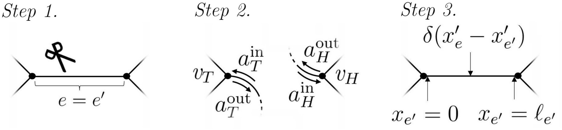
Figure 1. This three step procedure is described in detail below.

• Define the graph and the coordinate of the delta function excitation $\mathbf{x^{\prime}}=(e^{\prime},x^{\prime}_{e^{\prime}})$. The delta function acts as a source which we model by creating an auxiliary open scattering graph by “cutting out” the excited edge $e^{\prime}$ and replacing it with two auxiliary leads.

• Treat the auxiliary graph as a scattering site and construct a lead scattering matrix for energy $E_{+}$. This allows one to determine the two outgoing lead wave amplitudes in terms of the two incoming wave amplitudes which are free parameters.

• Take the scattering solution on the auxiliary leads at distances $x^{\prime}_{e^{\prime}}$ and $\ell_{e^{\prime}}-x^{\prime}_{e^{\prime}}$ from the vertices and ”glue” these solutions together such that the differential equation (25) is satisfied yielding a Dirac $\delta$-function at the position $\mathbf{x}^{\prime}$. This determines all free parameters and results in the Green’s function $G(\mathbf{x},\mathbf{x^{\prime}};E_{+})$.

Let us now go through these steps in detail:
Step 1. Consider a compact quantum graph $\mathcal{G}(\mathcal{V},\mathcal{E},L)$ as defined in Sec. 2 which we wish to excite with a delta function at location $\mathbf{x^{\prime}}=(e^{\prime},x^{\prime}_{e^{\prime}})\in\mathcal{G}$. Let us denote the vertex at $x_{e^{\prime}}=0$ as the ’tail’ vertex $v_{T}$ and the vertex at $x_{e^{\prime}}=l_{e^{\prime}}$ as the ’head’ vertex $v_{H}$. We begin by cutting the excited edge $e^{\prime}$ and replacing it by two leads attached at $v_{T}$ and $v_{H}$, respectively, thus creating the auxiliary open scattering graph $\mathcal{G}_{\mathrm{aux},e^{\prime}}=\mathcal{G}_{\mathrm{aux},e^{\prime}}(\mathcal{V},\mathcal{E}_{\mathrm{aux,e^{\prime}}},L_{\mathrm{aux,e^{\prime}}})$, where $\mathcal{E}_{\mathrm{aux,e^{\prime}}}=\mathcal{L}_{\mathrm{aux},e^{\prime}}\cup(\mathcal{B}\setminus\{e^{\prime}\})$ and $L_{\mathrm{aux},e^{\prime}}=L\setminus\{\ell_{e^{\prime}}\}$. The coordinates on the leads are set to be $x_{T}=x_{H}=0$ at the vertices $v_{T}$ and $v_{H}$, respectively. On each lead, the solutions are defined as

(27) $$\begin{split}&\psi_{T}(x_{T})=a_{T}^{\mathrm{in}}e^{-ik_{+}x_{T}}+a_{T}^{\mathrm{out}}e^{ik_{+}x_{T}},\\ &\psi_{H}(x_{H})=a_{H}^{\mathrm{in}}e^{-ik_{+}x_{H}}+a_{H}^{\mathrm{out}}e^{ik_{+}x_{H}}.\end{split}$$

Step 2. Next, we construct the scattering states on the auxiliary graph. The quantum map of the auxiliary graph can then be written in the form Eq. (18) and only differs from the quantum map (15) of $\mathcal{G}$ by excluding the rows corresponding to the excited edge $e^{\prime}$. The wave amplitudes on the two leads are mapped from incoming to outgoing wave amplitudes by the graph scattering matrix $\boldsymbol{\sigma}(k_{+})$ as defined in (20) with matrix elements

(28) $$\begin{pmatrix}a^{\mathrm{out}}_{\mathrm{H}}\\ a^{\mathrm{out}}_{\mathrm{T}}\end{pmatrix}=\begin{pmatrix}\sigma(k_{+})_{HH}&\sigma(k_{+})_{HT}\\ \sigma(k_{+})_{TH}&\sigma(k_{+})_{TT}\end{pmatrix}\begin{pmatrix}a^{\mathrm{in}}_{\mathrm{H}}\\ a^{\mathrm{in}}_{\mathrm{T}}\end{pmatrix}.$$

The incoming wave amplitudes $a^{\mathrm{in}}_{\mathrm{H}}$ and $a^{\mathrm{in}}_{\mathrm{T}}$ are at this stage free parameters.
Step 3. We project the set of scattering solutions from the auxiliary graph onto the original graph by cutting the leads $\mathrm{H}$ and $\mathrm{T}$ at $x_{\mathrm{T}}=x^{\prime}_{e^{\prime}}$ and $x_{\mathrm{H}}=\ell_{e^{\prime}}-x^{\prime}_{e^{\prime}}$, then ”gluing” the two ends together forming a single bond. The solution on $e^{\prime}$ is then

(29) $$\psi_{e^{\prime}}(x_{e^{\prime}})=\begin{cases}a^{\mathrm{in}}_{\mathrm{T}}e^{-ik_{+}x_{e^{\prime}}}+\left(\sigma_{\mathrm{TH}}a^{\mathrm{in}}_{\mathrm{H}}+\sigma_{\mathrm{TT}}a^{\mathrm{in}}_{\mathrm{T}}\right)e^{ik_{+}x_{e^{\prime}}}&\text{for $x_{e^{\prime}}<x^{\prime}_{e^{\prime}}$;}\\ a^{\mathrm{in}}_{\mathrm{H}}e^{-ik_{+}(\ell_{e^{\prime}}-x_{e^{\prime}})}+\left(\sigma_{\mathrm{HH}}a^{\mathrm{in}}_{\mathrm{H}}+\sigma_{\mathrm{HT}}a^{\mathrm{in}}_{\mathrm{T}}\right)e^{ik_{+}(\ell_{e^{\prime}}-x_{e^{\prime}})}&\text{for $x_{e^{\prime}}>x^{\prime}_{e^{\prime}}$.}\end{cases}$$

One determines $a^{\mathrm{in}}_{\mathrm{H}}$ and $a^{\mathrm{in}}_{\mathrm{T}}$ by fulfilling equation (25) at $x_{e^{\prime}}=x^{\prime}_{e^{\prime}}$; this leads to the following conditions:
i. continuity at $x_{e^{\prime}}=x^{\prime}_{e^{\prime}}$

(30) $$\lim_{\alpha\to 0^{+}}\left[\psi_{e^{\prime}}(x^{\prime}_{e^{\prime}}+\alpha)-\psi_{e^{\prime}}(x^{\prime}_{e^{\prime}}-\alpha)\right]=0;$$

ii. a discontinuity of the derivatives of the form

(31) $$\lim_{\alpha\to 0^{+}}\left[\frac{d\psi_{e^{\prime}}\left(x^{\prime}_{e^{\prime}}+\alpha\right)}{dx_{e^{\prime}}}-\frac{d\psi_{e^{\prime}}\left(x^{\prime}_{e^{\prime}}-\alpha\right)}{dx_{e^{\prime}}}\right]=1\ .$$

These two conditions result in a non-homogeneous system of linear equations for the two incoming scattering amplitudes. The unique solution of this system is

$$a^{\mathrm{in}}_{\mathrm{T}}= \frac{e^{ik_{+}\ell_{e^{\prime}}}\left(e^{-ik_{+}(\ell_{e^{\prime}}-x^{\prime}_{e^{\prime}})}+\sigma_{\mathrm{HH}}e^{ik_{+}(\ell_{e^{\prime}}-x^{\prime}_{e^{\prime}})}-\sigma_{\mathrm{TH}}e^{ik_{+}x^{\prime}_{e^{\prime}}}\right)}{2ik_{+}\left[(1-e^{ik_{+}\ell_{e^{\prime}}}\sigma_{\mathrm{HT}})(1-e^{ik_{+}\ell_{e^{\prime}}}\sigma_{\mathrm{TH}})-e^{2ik_{+}\ell_{e^{\prime}}}\sigma_{\mathrm{HH}}\sigma_{\mathrm{TT}})\right]}$$

(32a) $$= \frac{1}{2ik_{+}}\left[e^{ik_{+}x^{\prime}_{e^{\prime}}}\left[\frac{\mathbb{I}}{\mathbb{I}-\mathbf{U}(k_{+})}\right]_{e^{\prime}_{-}e^{\prime}_{-}}+e^{ik_{+}(\ell_{e^{\prime}}-x^{\prime}_{e^{\prime}})}\left[\frac{\mathbb{I}}{\mathbb{I}-\mathbf{U}(k_{+})}\right]_{e^{\prime}_{-}e^{\prime}_{+}}\right]$$

$$a^{\mathrm{in}}_{\mathrm{H}}= \frac{e^{ik_{+}\ell_{e^{\prime}}}\left(e^{-ik_{+}x^{\prime}_{e^{\prime}}}+\sigma_{\mathrm{TT}}e^{ik_{+}x^{\prime}_{e^{\prime}}}-\sigma_{\mathrm{HT}}e^{ik_{+}(\ell_{e^{\prime}}-x^{\prime}_{e^{\prime}})}\right)}{2ik_{+}\left[(1-e^{ik_{+}\ell_{e^{\prime}}}\sigma_{\mathrm{HT}})(1-e^{ik_{+}\ell_{e^{\prime}}}\sigma_{\mathrm{TH}})-e^{2ik_{+}\ell_{e^{\prime}}}\sigma_{\mathrm{HH}}\sigma_{\mathrm{TT}})\right]}$$

(32b) $$= \frac{1}{2ik_{+}}\left[e^{ik_{+}(\ell_{e^{\prime}}-x^{\prime}_{e^{\prime}})}\left[\frac{\mathbb{I}}{\mathbb{I}-\mathbf{U}(k_{+})}\right]_{e^{\prime}_{+}e^{\prime}_{+}}+e^{ik_{+}x^{\prime}_{e^{\prime}}}\left[\frac{\mathbb{I}}{\mathbb{I}-\mathbf{U}(k_{+})}\right]_{e^{\prime}_{+}e^{\prime}_{-}}\right]\ .$$

The derivation of the expressions involving $(\mathbb{I}-\mathbf{U}(k_{+}))^{-1}$, the resolvent matrix of the quantum map, can be found in A. Inserting (32) into (29) and extending the solution to the entire graph using (22), the Green’s function of the compact graph $\mathcal{G}$ can finally be written in the form

(33) $$G(\mathbf{x},\mathbf{x^{\prime}},E_{+})=\frac{1}{2k_{+}i} \left[\delta_{ee^{\prime}}e^{ik_{+}|x_{e}-x^{\prime}_{e^{\prime}}|}+e^{ik_{+}(x_{e}-x^{\prime}_{e^{\prime}}-\ell_{e}+\ell_{e^{\prime}})}\left[\frac{\mathbf{U}(k_{+})}{\mathbb{I}-\mathbf{U}(k_{+})}\right]_{e_{+}e^{\prime}_{+}}\right.$$

$$\;+e^{-ik_{+}(x_{e}-x^{\prime}_{e^{\prime}})}\left[\frac{\mathbf{U}(k_{+})}{\mathbb{I}-\mathbf{U}(k_{+})}\right]_{e_{-}e^{\prime}_{-}}$$

$$\;+e^{ik_{+}(x_{e}+x^{\prime}_{e^{\prime}}-\ell_{e})}\left[\frac{\mathbf{U}(k_{+})}{\mathbb{I}-\mathbf{U}(k_{+})}\right]_{e_{+}e^{\prime}_{-}}$$

$$\;+\left.e^{-ik_{+}(x_{e}+x^{\prime}_{e^{\prime}}-\ell_{e^{\prime}})}\left[\frac{\mathbf{U}(k_{+})}{\mathbb{I}-\mathbf{U}(k_{+})}\right]_{e_{-}e^{\prime}_{+}}\right].$$

This is our main result in this section. We give here for the first time a closed form expression of the Green’s function on a graph following the recipe from Barras and Gaspard [17].

By formally expanding $\frac{\mathbf{U}}{\mathbb{I}-\mathbf{U}}=\sum_{n=1}^{\infty}\mathbf{U}^{n}$, one may express the Green’s function as a sum over paths $p$ on the metric graph starting at $\mathbf{x}^{\prime}$ and ending at $\mathbf{x}$, that is,

(34) $$G(\mathbf{x},\mathbf{x^{\prime}},E_{+})=\frac{1}{2k_{+}i}\sum_{p}A_{p}(k_{+})e^{iL_{p}k_{+}}\,.$$

Here, $L_{p}$ is the metric length of the path and the amplitude $A_{p}$ is the product of all scattering amplitudes along the trajectory. If $e=e^{\prime}$, the direct path between $x_{e^{\prime}}$ and $x^{\prime}_{e^{\prime}}$ has $L_{p}=|x_{e^{\prime}}-x^{\prime}_{e^{\prime}}|$ and $A_{p}=1$. Eq. (34) is the starting point for the investigations in [17], which, however, makes it necessary to do an explicit summation over all possible paths - in general a cumbersome task. Note also that this expansion converges only if the imaginary part of $k_{+}$ is positive and these expressions thus require a limit if used for real wave numbers. This is all well known for similar expansions into sums over paths in trace formulae and scattering systems, we refer to the textbook [8] and references therein.

Finally, let us shortly discuss the pole structure of the Green’s function. For a compact graph, the eigenvalue spectrum is a discrete countable set $\{E_{0},E_{1},\dots\}$. Let us assume that there are no degeneracies and all eigenvalues are positive, that is, $E_{n}>0$. The spectral decomposition of the Schrödinger operator $\hat{H}$ allows us to write the resolvent operator as

(35) $$(E_{+}-\hat{H})^{-1}=\sum_{n=0}^{\infty}\frac{\hat{P}_{n}}{E_{+}-E_{n}}$$

where $\hat{P}_{n}$ is the projection operator onto the subspace spanned by the $n$-th eigenvector. For the Green’s function this implies

(36) $$G(\mathbf{x},\mathbf{x^{\prime}},E_{+})=\sum_{n=0}^{\infty}\frac{P_{n}(\mathbf{x},\mathbf{x^{\prime}})}{E_{+}-E_{n}}$$

where $P_{n}(\mathbf{x},\mathbf{x^{\prime}})$ is the integral kernel of $\hat{P}_{n}$. Let us now show that (33) and (36) are indeed equivalent. We start by considering the limit $E_{+}\to E_{n}$ for some given eigenvalue $E_{n}=k_{n}^{2}$ and by showing that the singular part of the Green’s function (33) in this limit is given by $\frac{P_{n}(\mathbf{x},\mathbf{x^{\prime}})}{E_{+}-E_{n}}$. Let us extract first the singular part of the matrix

(37) $$\frac{\mathbf{U}(k_{+})}{\mathbb{I}-\mathbf{U}(k_{+})}\sim\frac{\mathbf{P}}{-i(k_{+}-k_{n})C}\ .$$

Here, $\mathbf{P}=\mathbf{b}^{\mathrm{in}}{\mathbf{b}^{\mathrm{in}}}^{\dagger}$ is the projection matrix with matrix elements on the corresponding unit eigenvector $\mathbf{U}(k_{n})\mathbf{b}^{\mathrm{in}}=\mathbf{b}^{\mathrm{in}}$ and

(38) $$C={\mathbf{b}^{\mathrm{in}}}^{\dagger}\left[k_{n}\mathbf{L}+\sin(k_{n}\mathbf{L})\boldsymbol{\Pi}\right]\mathbf{b}^{\mathrm{in}}>0$$

is a positive constant and $\mathbf{L}$ is a $2{N}_{B}$ dimensional diagonal matrices with diagonal entries $\ell_{e}$. We refer to B for a detailed derivation of (37) and (38). With $2k_{+}(k_{+}-k_{n})\sim E_{+}-E_{n}$ one then finds

$$G(\mathbf{x},\mathbf{x^{\prime}},E_{+})\sim \frac{\big{(}a_{e_{-}}^{\mathrm{in}}e^{-ik_{n}x_{e}}+a_{e_{+}}^{\mathrm{in}}e^{ik_{n}(x_{e}-\ell_{e})}\big{)}^{*}\big{(}a_{e^{\prime}_{-}}^{\mathrm{in}}e^{-ik_{n}x_{e^{\prime}}}+a_{e^{\prime}_{+}}^{\mathrm{in}}e^{ik_{n}(x_{e^{\prime}}-\ell_{e^{\prime}})}\big{)}}{C(E_{+}-E_{n})}$$

(39) $$= \frac{P_{n}(\mathbf{x},\mathbf{x^{\prime}})}{E_{+}-E_{n}}\ ,$$

where the last equality requires that the constant $C$ gives the correct normalization of the projection kernel $P_{n}(\mathbf{x},\mathbf{x^{\prime}})$. This is equivalent to $\sum_{e\in\mathcal{E}}\int_{0}^{\ell_{e}}P_{n}((e,x_{e}),(e,x_{e}))dx_{e}=1$ which is easily checked by direct calculation. Repeating this calculation for $E_{+}$ near to all other energy eigenvalues shows that expressions (33) and (36) have the same poles and the same residues. Both expressions can be continued analytically to the lower half plane where the imaginary part of the energy is negative. They are thus equivalent up to an entire function $F(E)$, (i.e., it is analytic in the whole complex plane). As both (33) and (36) vanish in the limit $E_{i}\to\pm\infty$, the same must be true for their difference $F(E)$. The entire function that vanishes in these limits for all $E_{r}$ is $F(E)=0$.

3.2. Construction of the Green’s function for open scattering graphs

The construction of the Green’s function on an open scattering graph follows analogously. In this case, our assumption that the energy has a positive imaginary part together with the requirement of square integrability leads to outgoing boundary conditions along the leads. That is, the amplitudes of incoming plane waves need to vanish, as these would lead to exponentially increasing contributions. These conditions are straight forward to implement and we can go through the same construction as for the compact graph. A short-cut is obtained by first replacing each lead $e\in\mathcal{L}$ by an edge of finite length with a dangling vertex of degree one and choosing some self-adjoint boundary conditions at the dangling vertices. This results in an auxiliary compact quantum graph as described in the previous section. The Green’s function of the auxiliary quantum graph is then given by (33). Clearly, the solution depends on the lengths that have been introduced for the leads as parameters. Next, one sends the introduced edge lengths to infinity. Because the imaginary part of the wave number is positive $\mathrm{Im}\ k_{+}>0$ the corresponding phase factors then decay as $e^{ik_{+}\ell_{e}}\to 0$ as $\ell_{e}\to\infty$. In this limit any dependence on the arbitrary choice of boundary conditions at the dangling vertices disappears and what remains is the Green’s function of the open graph. We refer to C for the details of the calculation which results in

(40) $$G(\mathbf{x},\mathbf{x^{\prime}},E_{+})=\frac{1}{2k_{+}i}\times\\ \begin{cases}\delta_{e,e^{\prime}}\,e^{ik_{+}|x_{e}-x^{\prime}_{e^{\prime}}|}+e^{ik_{+}(x_{e}+x^{\prime}_{e^{\prime}})}\left[\mathbf{U}(k_{+})_{\mathcal{LL}}+\mathbf{U}(k_{+})_{\mathcal{LB}}\frac{\mathbb{I}}{\mathbb{I}-\mathbf{U}(k_{+})_{\mathcal{BB}}}\mathbf{U}(k_{+})_{\mathcal{BL}}\right]_{ee^{\prime}}\\ \qquad\hfill\text{if $e,e^{\prime}\in\mathcal{L}$,\qquad\; \quad}\\[14.22636pt] e^{ik_{+}(x_{e}-x^{\prime}_{e^{\prime}}+\ell_{e^{\prime}})}\left[\mathbf{U}(k_{+})_{\mathcal{LB}}\frac{\mathbb{I}}{\mathbb{I}-\mathbf{U}(k_{+})_{\mathcal{BB}}}\right]_{ee^{\prime}_{+}}+e^{ik_{+}(x_{e}+x^{\prime}_{e^{\prime}})}\left[\mathbf{U}(k_{+})_{\mathcal{LB}}\frac{\mathbb{I}}{\mathbb{I}-\mathbf{U}(k_{+})_{\mathcal{BB}}}\right]_{ee^{\prime}_{-}}\\ \qquad\hfill\text{if $e\in\mathcal{L}$ and $e^{\prime}\in\mathcal{B}$,}\\[14.22636pt] e^{-ik_{+}(x_{e}-x^{\prime}_{e^{\prime}})}\left[\frac{\mathbb{I}}{\mathbb{I}-\mathbf{U}(k_{+})_{\mathcal{BB}}}\mathbf{U}(k_{+})_{\mathcal{BL}}\right]_{e_{-}e^{\prime}}+e^{ik_{+}(x_{e}+x^{\prime}_{e^{\prime}}-\ell_{e})}\left[\frac{\mathbb{I}}{\mathbb{I}-\mathbf{U}(k_{+})_{\mathcal{BB}}}\mathbf{U}(k_{+})_{\mathcal{BL}}\right]_{e_{+}e^{\prime}}\\ \qquad\hfill\text{if $e\in\mathcal{B}$ and $e^{\prime}\in\mathcal{L}$,}\\[14.22636pt] \delta_{ee^{\prime}}\,e^{ik_{+}|x_{e}-x^{\prime}_{e^{\prime}}|}+e^{ik_{+}(x_{e}-x^{\prime}_{e^{\prime}}-\ell_{e}+\ell_{e^{\prime}})}\left[\frac{\mathbf{U}(k_{+})_{\mathcal{BB}}}{\mathbb{I}-\mathbf{U}(k_{+})_{\mathcal{BB}}}\right]_{e_{+}e^{\prime}_{+}}+e^{-ik_{+}(x_{e}-x^{\prime}_{e^{\prime}})}\left[\frac{\mathbf{U}(k_{+})_{\mathcal{BB}}}{\mathbb{I}-\mathbf{U}(k_{+})_{\mathcal{BB}}}\right]_{e_{-}e^{\prime}_{-}}\\[2.84544pt] \ +\,e^{ik_{+}(x_{e}+x^{\prime}_{e^{\prime}}-\ell_{e})}\left[\frac{\mathbf{U}(k_{+})_{\mathcal{BB}}}{\mathbb{I}-\mathbf{U}(k_{+})_{\mathcal{BB}}}\right]_{e_{+}e^{\prime}_{-}}+e^{-ik_{+}(x_{e}+x^{\prime}_{e^{\prime}}-\ell_{e^{\prime}})}\left[\frac{\mathbf{U}(k_{+})_{\mathcal{BB}}}{\mathbb{I}-\mathbf{U}(k_{+})_{\mathcal{BB}}}\right]_{e_{-}e^{\prime}_{+}}\\ \qquad\hfill\text{if $e,e^{\prime}\in\mathcal{B}$.\qquad\; \quad}\end{cases}$$

If the energy spectrum of the graph is continuous these expressions are regular and the limit $\mathrm{Im}\ k_{+}\to 0^{+}$ can be performed by just choosing $k_{+}\to k\in\mathbb{R}$. A similar expression for energies $E_{-}^{2}=k_{-}^{2}$ with negative imaginary parts may be obtained in the same way. More directly, it can be obtained from the symmetry (26). Note that it will have a different limit as $k_{-}$ approaches the real axis.
The energy spectrum of an open graph may contain a discrete set $\{E_{0},E_{1},\dots\}$ of bound states in the continuum. These have square integrable eigenfunctions and they thus vanish on the leads. The Green’s function for $E$ close to any of these energy eigenvalues will have poles just as in the compact case that we discussed in the previous section. And the calculation there applies here as well. If either $\mathbf{x}$ or $\mathbf{x^{\prime}}$ is chosen on a lead the expression for the Green’s function should remain regular as $E\to E_{n}=k_{n}^{2}$ which is not obvious from the given explicit expressions above which contain the inverse $\left(\mathbb{I}-U(k_{+})_{\mathcal{BB}}\right)^{-1}$. We will show regularity explicitly if both $\mathbf{x}$ and $\mathbf{x^{\prime}}$ are on the leads. In that case the expression above reduces to

(41) $$G(\mathbf{x},\mathbf{x^{\prime}},E_{+})=\frac{1}{2k_{+}i}\left[\delta_{e,e^{\prime}}\,e^{ik_{+}|x_{e}-x^{\prime}_{e^{\prime}}|}+e^{ik_{+}(x_{e}+x^{\prime}_{e^{\prime}})}\boldsymbol{\sigma}(k_{+})_{e,e^{\prime}}\right]\ .$$

We will show in the following section that the scattering matrix is indeed regular as $k\to k_{n}$ for at a bound state. Regularity in the case that one point is on a lead and the other on a bond can be shown as well using essentially the same tools but we will leave this to the reader.

4. Regularisation schemes for perfect scars

4.1. Bound states in the continuum

The eigenstates of a quantum graph are generally supported on all edges of a graph as long as the graph is fully connected. However, it is not too difficult to construct graphs which have eigenstates that are non-zero exclusively on a compact subgraph $\mathcal{S}$, but vanish exactly on the rest $\mathcal{R}$ of the edges. We call such an eigenstate a perfect scar of the graph. These states exist, for example, on quantum graphs with Kirchhoff-Neumann conditions where the subgraph $\mathcal{S}$ is a cycle on which all edge lengths are rationally dependent. In that case, the cycle edge lengths are an integer multiple of a minimal length $\ell_{e}=n_{e}\ell_{0}$. At wave number $\tilde{k}=2\pi/\ell_{0}$ (or any integer multiple of it), one may then set

(42) $$\psi_{e}(x_{e})=\begin{cases}\pm\sin(\tilde{k}x_{e})&\text{if $e$ belongs to the cycle of $\mathcal{S}$;}\\ 0&\text{if e belongs to $\mathcal{R}$}.\end{cases}$$

Here the signs $\pm$ can be chosen to satisfy the flux conservation condition.

Since the union of $\mathcal{S}$ and $\mathcal{R}$ make up the total graph $\mathcal{G}$, it is natural to express the quantum map in the block-form

(43) $$\mathbf{U}(k)=\begin{pmatrix}\mathbf{U}(k)_{\mathcal{RR}}&\mathbf{U}(k)_{\mathcal{RS}}\\ \mathbf{U}(k)_{\mathcal{SR}}&\mathbf{U}(k)_{\mathcal{SS}}\end{pmatrix}$$

with appropriate permutations applied. In general there is perfect scar on the subgraph $\mathcal{S}$ at energy $E=k^{2}>0$, if the block $\mathbf{U}(k)_{\mathcal{SS}}$ has an eigenvector $\mathbf{a}_{\mathcal{S}}^{\mathrm{in}}$ with unit eigenvalue $\mathbf{U}(k)_{\mathcal{SS}}\mathbf{a}_{S}^{\mathrm{in}}=\mathbf{a}_{\mathcal{S}}^{\mathrm{in}}$. The unitarity of the full quantum map then implies that $\mathbf{U}(k)_{\mathcal{RS}}\mathbf{a}_{\mathcal{S}}^{\mathrm{in}}=0$ vanishes. One may extend $\mathbf{a}_{\mathcal{S}}^{\mathrm{in}}$ to an eigenvector of the full map by setting $\mathbf{a}_{\mathcal{R}}^{\mathrm{in}}=0$ resulting in the vanishing of wave amplitudes on edges that do not belong to $\mathcal{S}$.

For open graphs, a perfect scar at a wavenumber $k_{0}>0$ is a bound state in the continuum and this situation is again straight forward to construct, such as by using the cycle example above. In this case, one may take $\mathcal{R}$ to contain all leads and $\mathcal{S}$ to be a sub-graph containing a sub-set of the finite bonds.

Throughout the previous sections, we assumed that the matrix $\mathbb{I}-\mathbf{U}(k)_{\mathcal{BB}}$ is invertible, which it is generically the case as $\mathbf{U}(k)_{\mathcal{BB}}$ is a block of a unitary matrix. However, a perfect scar exists, if and only if $\mathbf{U}(k)_{\mathcal{BB}}$ has an eigenvalue one at the wave number $k=k_{0}$. Even in the case of “almost” perfect scars (with small nonzero entries for $\mathbf{a}_{\mathcal{R}}^{\mathrm{in}}$), matrix inversion may cause large numerical errors when inverting $\mathbb{I}-\mathbf{U}(k)_{\mathcal{BB}}$. To deal with this issue, we describe a regularisation scheme of the scattering matrix in the following section. This is important when dealing with open quantum graphs and when constructing Green’s function both in the compact and open case. The approach may also be used to find the regular part of the Green’s function in compact quantum graphs when the energy is in the eigenvalue spectrum. (By regular part, we refer to the Green’s function where the contribution from the pole at the energy has been removed). We will focus on the regularization of the scattering matrix, as the other applications can all be derived from there when needed.

4.2. Regularization of the scattering approach at a bound state

We will show in this section that scattering solutions of the form (20) are well defined at $k=k_{0}$ even in the presence of a bound state at that wave number. We show in D that the scattering matrix can be regularised across a whole $k$ interval containing $k_{0}$.

Consider a non-degenerate bound state at wave number $k=k_{0}$ with wave amplitudes $\mathbf{b}_{\mathcal{B}}^{\mathrm{in}}$ such that,

(44) $$\mathbf{U}(k_{0})_{\mathcal{BB}}\,\mathbf{b}_{\mathcal{B}}^{\mathrm{in}}=\mathbf{b}_{\mathcal{B}}^{\mathrm{in}}\ .$$

As discussed in the previous section, the unitarity of the quantum map $\mathbf{U}(k)$ implies

(45) $$\mathbf{U}(k_{0})_{\mathcal{LB}}\mathbf{b}_{\mathcal{B}}^{\mathrm{in}}=0\qquad\text{and}\qquad{\mathbf{b}_{\mathcal{B}}^{\mathrm{in}}}^{\dagger}\mathbf{U}(k_{0})_{\mathcal{BL}}=0,$$

that is, incoming waves $\mathbf{a}^{\mathrm{in}}_{\mathcal{L}}$ in the leads can not couple into the bound state $\mathbf{b}_{\mathcal{B}}^{\mathrm{in}}$ and the bound state can not couple back out. Let us assume for simplicity that the perfect scar described by $\mathbf{b}_{\mathcal{B}}^{\mathrm{in}}$ is not degenerate and introduce the idempotent, Hermitian $2N_{\mathcal{B}}\times 2N_{\mathcal{B}}$ projection matrix

(46) $$\mathbf{P}\equiv\mathbf{b}_{\mathcal{B}}^{\mathrm{in}}{\mathbf{b}_{\mathcal{B}}^{\mathrm{in}}}^{\dagger}$$

and its orthogonal complement

(47) $$\mathbf{Q}=\mathbb{I}-\mathbf{P}\ .$$

The methods below can be generalised to situations where more than one perfect scar exists at the same wave number $k_{0}$, such as, if all edge lengths are rationally related in a large graph with Neumann-Kirchhoff matching conditions. Writing Eq. (22) in the form

(48) $$\left(\mathbb{I}-\mathbf{U}(k)_{\mathcal{BB}}\right)\mathbf{a}^{\mathrm{in}}_{\mathcal{B}}=\mathbf{U}(k)_{\mathcal{BL}}\mathbf{a}^{\mathrm{in}}_{\mathcal{L}},$$

we find that the solution $\mathbf{a}^{\mathrm{in}}_{\mathcal{B}}$ is not unique at $k=k_{0}$ as both

(49) $$\mathbf{P}\left(\mathbb{I}-\mathbf{U}(k_{0})_{\mathcal{BB}}\right)=0\quad\mbox{and}\quad\mathbf{P}\mathbf{U}(k_{0})_{\mathcal{BL}}=0,$$

which follows directly from (45). This implies, that for any solution $\mathbf{a}^{\mathrm{in}}_{\mathcal{B}}$ of Eq. (48), $\mathbf{a}^{\mathrm{in}}_{\mathcal{B}}+\alpha\mathbf{b}_{\mathcal{B}}^{\mathrm{in}}$, $\alpha\in\mathbb{C}$, is also a solution. However, a unique solution $\tilde{\mathbf{a}}^{\mathrm{in}}_{\mathcal{B}}$ exists for the reduced system of equations

(50) $$\mathbf{Y}_{Q}(k_{0})\,\tilde{\mathbf{a}}^{\mathrm{in}}_{\mathcal{B}}=\mathbf{U}(k_{0})_{\mathcal{BL}}\,\mathbf{a}^{\mathrm{in}}_{\mathcal{L}}\quad\mbox{with}\quad\mathbf{Y}_{Q}(k_{0})=\mathbf{Q}\left(\mathbb{I}-\mathbf{U}(k_{0})_{\mathcal{BB}}\right)\mathbf{Q}.$$

As $\mathbf{Y}_{Q}(k_{0})\mathbf{b}_{\mathcal{B}}^{\mathrm{in}}=0$, its standard inverse does not exist. One may invert it in the subspace orthogonal to $\mathbf{b}_{\mathcal{B}}^{\mathrm{in}}$. Let us define (with mild abuse of notation)

(51) $$\mathbf{Y}_{Q}(k_{0})^{-1}=\mathbf{Q}\frac{\mathbb{I}}{\mathbb{I}-\mathbf{QU}(k_{0})\mathbf{Q}}\mathbf{Q}$$

as the unique $2N_{\mathcal{B}}\times 2N_{\mathcal{B}}$ matrix with by $\mathbf{Y}_{Q}(k_{0})^{-1}\mathbf{Y}_{Q}(k_{0})=\mathbf{Q}=\mathbf{Y}_{Q}(k_{0})\mathbf{Y}_{Q}(k_{0})^{-1}$ and $\mathbf{Y}_{Q}(k_{0})^{-1}\mathbf{P}=0=\mathbf{P}\mathbf{Y}_{Q}(k_{0})^{-1}$. As $\mathbf{U}(k_{0})_{\mathcal{LB}}\mathbf{P}=0$, one obtains a well-defined scattering solution for Eq. (20), that is,

(52) $$\mathbf{a}(k)^{\mathrm{out}}_{\mathcal{L}}=\mathbf{U}(k_{0})_{\mathcal{LB}}\,\tilde{\mathbf{a}}^{\mathrm{in}}_{\mathcal{B}}.$$

We may thus write the scattering matrix (21) in the form

(53) $$\boldsymbol{\sigma}(k_{0})=\mathbf{U}(k_{0})_{\mathcal{LL}}+\mathbf{U}(k_{0})_{\mathcal{LB}}\mathbf{Y}_{Q}(k_{0})^{-1}\mathbf{U}(k_{0})_{\mathcal{BL}}\ .$$

For an in-depth discussion of the regularity of the scattering matrix as $k\to k_{0}$, see D.

5. Worked examples

In this section we explicitly construct the scattering matrices of two open quantum graphs which contain perfect scars. Expressions for the Green’s function on the leads follow directly using (41).

5.1. Open lasso

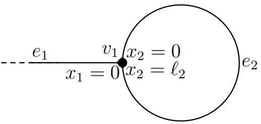
Figure 2. An open lasso graph constructed from two edges $e_{1}$ and $e_{2}$ where $e_{1}$ is a lead and $e_{2}$ is an bond. Both edges are connected to the same vertex $v_{1}$ where edge $e_{2}$ has both ends connected forming a loop wherein bound states can exist in the continuum.

Consider the open lasso quantum graph illustrated in figure 2. The coordinate $x_{1}\geq 0$ runs along the lead with $x_{1}=0$ at the vertex $v_{1}$ and the coordinate $x_{2}\in[0,\ell_{2}]$ runs along the loop such that $x_{2}=0$ and $x_{2}=\ell_{2}$ are the endpoints at the vertex $v_{1}$. At the vertex, we enforce Neumann boundary conditions, as expressed in (10), leading to the quantum map written in block form as

(54) $$\mathbf{U}(k)=\begin{pmatrix}\begin{array}[]{c|cc}-\frac{1}{3}&\frac{2}{3}&\frac{2}{3}\\[2.84544pt] \hline\cr\rule{0.0pt}{15.6491pt}\frac{2e^{ik\ell_{2}}}{3}&\frac{2e^{ik\ell_{2}}}{3}&-\frac{e^{ik\ell_{2}}}{3}\\[2.84544pt] \frac{2e^{ik\ell_{2}}}{3}&-\frac{e^{ik\ell_{2}}}{3}&\frac{2e^{ik\ell_{2}}}{3}\end{array}\end{pmatrix}\equiv\begin{pmatrix}\mathbf{U}_{\mathcal{LL}}&\mathbf{U}_{\mathcal{LB}}\\ \mathbf{U}(k)_{\mathcal{BL}}&\mathbf{U}(k)_{\mathcal{BB}}\\ \end{pmatrix}.$$

In the construction of the scattering matrix and the Green’s function, one needs to invert the matrix $\mathbb{I}-\mathbf{U}(k)_{\mathcal{BB}}$ which yields

(55) $$\frac{\mathbb{I}}{\mathbb{I}-\mathbf{U}(k)_{\mathcal{BB}}}=\begin{pmatrix}\frac{3-2e^{ik\ell_{2}}}{\left(e^{ik\ell_{2}}-1\right)\left(e^{ik\ell_{2}}-3\right)}&-\frac{e^{ik\ell_{2}}}{\left(e^{ik\ell_{2}}-1\right)\left(e^{ik\ell_{2}}-3\right)}\\[8.5359pt] -\frac{e^{ik\ell_{2}}}{\left(e^{ik\ell_{2}}-1\right)\left(e^{ik\ell_{2}}-3\right)}&\frac{3-2e^{ik\ell_{2}}}{\left(e^{ik\ell_{2}}-1\right)\left(e^{ik\ell_{2}}-3\right)}\end{pmatrix}$$

and is well defined as long as $e^{ik\ell_{2}}\neq 1$, that is, if $k\neq k_{n}=2\pi n/\ell_{2}$ for $n=1,2,\dots$. The reason for this is the existence of perfect scars on the loop which here lead to bound states in the continuum of scattering states. These bound state wave functions are given as

(56a) $$\psi_{e_{1}}(x_{1})= 0,$$

(56b) $$\psi_{e_{2}}(x_{2})= \sqrt{\frac{2}{\ell_{2}}}\sin(k_{n}x_{2})\ .$$

The continuum of scattering states exists for all wave numbers $k>0$ and is given by

(57a) $$\psi_{e_{1}}(x_{1})= e^{-ikx_{1}}+\boldsymbol{\sigma}(k)e^{ikx_{1}},$$

(57b) $$\psi_{e_{2}}(x_{2})= \boldsymbol{\rho}(k)_{2_{+}1}e^{ik(x_{2}-\ell_{2})}+\boldsymbol{\rho}(k)_{2_{-}1}e^{-ikx_{2}}\ .$$

where

(58) $$\boldsymbol{\rho}(k)=\frac{\mathbb{I}}{\mathbb{I}-\mathbf{U}(k)_{\mathcal{BB}}}\mathbf{U}(k)_{\mathcal{BL}}=\begin{pmatrix}\frac{2e^{ik\ell_{2}}}{3-e^{ik\ell_{2}}}\\[2.84544pt] \frac{2e^{ik\ell_{2}}}{3-e^{ik\ell_{2}}}\end{pmatrix}$$

and

(59) $$\boldsymbol{\sigma}(k)=\mathbf{U}_{\mathcal{LL}}+\mathbf{U}_{\mathcal{LB}}\boldsymbol{\rho}(k)=\frac{3e^{ik\ell_{2}}-1}{3-e^{ik\ell_{2}}}\ .$$

While the matrix $\frac{\mathbb{I}}{\mathbb{I}-\mathbf{U}(k)_{\mathcal{BB}}}$ is used to find $\boldsymbol{\rho}(k)$ and $\boldsymbol{\sigma}(k)$ in the scattering approach the poles at $k=k_{n}$ have disappeared in the final results. Note that bound states and scattering states are trivially orthogonal due to their symmetry under $x_{2}\mapsto\ell_{2}-x_{2}$ (which can be viewed as a mirror symmetry of the lasso). The bound states are odd under this symmetry as $\psi_{1}(x_{1})=0$ and $\psi_{2}(x_{2})=-\psi_{2}(\ell_{2}-x_{2})$ at wave numbers $k_{n}$. The scattering states are even under this symmetry for all wave numbers $k>0$ as

(60) $$\psi_{e_{2}}(x_{2})=\frac{4e^{ik\ell_{2}/2}}{3-e^{ik\ell_{2}}}\cos\left(k\frac{2x_{2}-\ell_{2}}{2}\right)=\psi_{2}(\ell_{2}-x_{2}).$$

For completeness, we give the full Green’s function for this example below, where $x_{e}$ (or $x^{\prime}_{e^{\prime}}$) are either on the lead ($e=e_{1}$) or on the loop ($e=e_{2}$). Following on from the last line in (40), one obtains, using the expressions in (54) and (55),

(61) $$G_{\mathrm{lasso}}(\mathbf{x},\mathbf{x^{\prime}},E_{+})=\frac{1}{2k_{+}i}\times\\ \begin{cases}e^{ik_{+}|x_{e}-x^{\prime}_{e^{\prime}}|}+e^{ik_{+}(x_{e}+x^{\prime}_{e^{\prime}})}\frac{3e^{ik_{+}\ell_{2}}-1}{3-e^{ik_{+}\ell_{2}}}&\text{if $e=e_{1}$ and $e^{\prime}=e_{1}$,}\\[14.22636pt] \frac{2}{3-e^{ik_{+}\ell_{2}}}e^{ik_{+}x_{e_{1}}}\left(e^{ik_{+}x^{\prime}_{e_{2}}}+e^{-ik_{+}(x^{\prime}_{e_{2}}-\ell_{2})}\right)&\text{if $e=e_{1}$ and $e^{\prime}=e_{2}$,}\\[14.22636pt] \frac{2}{3-e^{ik_{+}\ell_{2}}}e^{ik_{+}x^{\prime}_{e_{1}}}\left(e^{-ik_{+}x_{e_{2}}}+e^{ik_{+}(x_{e_{2}}-\ell_{2})}\right)&\text{if $e=e_{2}$ and $e^{\prime}=e_{1}$,}\\[14.22636pt] \,e^{ik_{+}|x_{e_{2}}-x^{\prime}_{e_{2}}|}+\frac{2e^{ik_{+}\ell_{2}}}{(e^{ik_{+}\ell_{2}}-1)(e^{ik_{+}\ell_{2}}-3)}\left[(2-e^{ik_{+}\ell_{2}})\cos(k_{+}(x_{e_{2}}-x^{\prime}_{e_{2}}))\right.\\ \qquad\left.-\cos(k_{+}(x_{e_{2}}+x^{\prime}_{e_{2}}-\ell_{2}))\right]&\text{if $e=e_{2}$ and $e^{\prime}=e_{2}$.}\\[14.22636pt] \end{cases}$$

5.2. Scattering states for an open 3-star with one lead

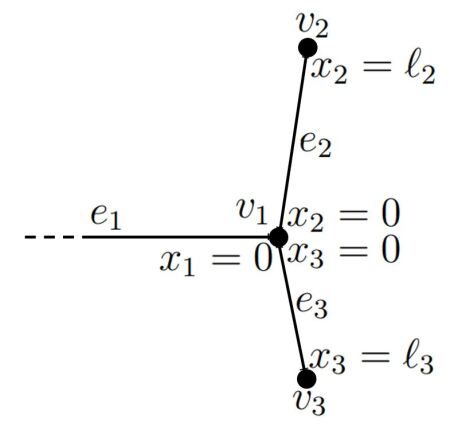
Figure 3. A 3-star with one lead consists of a central vertex $v_{1}$ with three edges $e_{n},n=1,2,3$, attached. Here, $e_{1}$ is a lead and the other two edges $e_{2}$ and $e_{3}$ are bonds of lengths $\ell_{2}$ and $\ell_{3}$ ending in vertices $v_{2}$ and $v_{3}$.

Consider the open T-junction quantum graph as illustrated in Figure 3. We choose the three coordinates such that $x_{n}=0$ for $n=1,2,3$ at the central vertex $v_{1}$ with $x_{n}=\ell_{n}$ at vertices $v_{n},n=2,3$. We enforce Kirchhoff-Neumann boundary conditions at the central vertex as expressed in (10) and Dirichlet boundary conditions at $v_{2},v_{3}$, that is, $\Sigma^{(v_{n})}=-1,n=2,3$, leading to the quantum map

(62) $$\mathbf{U}(k)=\begin{pmatrix}\begin{array}[]{c|cccc}-\frac{1}{3}&0&0&\frac{2}{3}&\frac{2}{3}\\[2.84544pt] \hline\cr\rule{0.0pt}{14.22636pt}\frac{2e^{ik\ell_{2}}}{3}&0&0&-\frac{e^{ik\ell_{2}}}{3}&\frac{2e^{ik\ell_{2}}}{3}\\ \frac{2e^{ik\ell_{3}}}{3}&0&0&\frac{2e^{ik\ell_{3}}}{3}&-\frac{e^{ik\ell_{3}}}{3}\\ 0&-e^{ik\ell_{2}}&0&0&0\\ 0&0&-e^{ik\ell_{3}}&0&0\end{array}\end{pmatrix}\equiv\begin{pmatrix}\mathbf{U}_{\mathcal{LL}}&\mathbf{U}_{\mathcal{LB}}\\ \mathbf{U}(k)_{\mathcal{BL}}&\mathbf{U}(k)_{\mathcal{BB}}\\ \end{pmatrix}.$$

Computing the scattering matrix and Green’s function in the scattering approach require that one inverts the matrix $\mathbb{I}-\mathbf{U}(k)_{\mathcal{BB}}$ which is given as

(63) $$\begin{split}&\frac{\mathbb{I}}{\mathbb{I}-\mathbf{U}(k)_{\mathcal{BB}}}=\\ &\frac{1}{D}\begin{pmatrix}3-e^{2ik\ell_{3}}&-2e^{ik(\ell_{2}+\ell_{3})}&-(1+e^{2ik\ell_{3}})e^{ik\ell_{2}}&2e^{ik\ell_{2}}\\ -2e^{ik(\ell_{2}+\ell_{3})}&3-e^{2ik\ell_{2}}&2e^{ik\ell_{3}}&-(1+e^{2ik\ell_{2}})e^{ik\ell_{3}}\\ -(3-e^{2ik\ell_{3}})e^{ik\ell_{2}}&2e^{ik(2\ell_{2}+\ell_{3})}&3-e^{2ik\ell_{3}}&-2e^{2ik\ell_{2}}\\ 2e^{ik(\ell_{2}+2\ell_{3})}&-(3-e^{2ik\ell_{2}})e^{ik\ell_{3}}&-2e^{2ik\ell_{3}}&3-e^{2ik\ell_{2}}\end{pmatrix}\end{split}$$

where

(64) $$D=3-e^{2ik\ell_{2}}-e^{2ik\ell_{3}}-e^{2ik(\ell_{2}+\ell_{3})}\ .$$

Note that for $e^{2ik\ell_{2}}=e^{2ik\ell_{3}}=1$, one has $D=0$ making the inverse not well defined. This can only happen if the bond lengths are rationally related, then giving rise to a set of bound state in the continuum that vanish on the lead and are a sinusoidal wave along the two bonds with a node on the vertex $v_{1}$. In either case the scattering states are given by

(65a) $$\psi_{e_{1}}(x_{1})= e^{-ikx_{1}}+\boldsymbol{\sigma}(k)e^{ikx_{1}},$$

(65b) $$\psi_{e_{2}}(x_{2})= \boldsymbol{\rho}(k)_{2_{+}1}e^{ik(x_{2}-\ell_{2})}+\boldsymbol{\rho}(k)_{2_{-}1}e^{-ikx_{2}}$$

(65c) $$\psi_{e_{3}}(x_{3})= \boldsymbol{\rho}(k)_{3_{+}1}e^{ik(x_{3}-\ell_{3})}+\boldsymbol{\rho}(k)_{3_{-}1}e^{-ikx_{3}}$$

where

(66) $$\boldsymbol{\rho}(k)=\frac{\mathbb{I}}{\mathbb{I}-\mathbf{U}(k)_{\mathcal{BB}}}\mathbf{U}(k)_{\mathcal{BL}}=\frac{2}{D}\begin{pmatrix}e^{ik\ell_{2}}\left(1-e^{2ik\ell_{3}}\right)\\ e^{ik\ell_{3}}\left(1-e^{2ik\ell_{2}}\right)\\ -e^{2ik\ell_{2}}\left(1-e^{2ik\ell_{3}}\right)\\ -e^{2ik\ell_{3}}\left(1-e^{2ik\ell_{2}}\right)\end{pmatrix}$$

and

(67) $$\boldsymbol{\sigma}(k)=\mathbf{U}_{\mathcal{LL}}+\mathbf{U}_{\mathcal{LB}}\boldsymbol{\rho}(k)=\frac{D^{*}}{D}e^{2ik(\ell_{2}+\ell_{3})}\ .$$

The scattering states are then given as

(68a) $$\psi_{e_{1}}(x_{1})= e^{-ikx_{1}}+\frac{D^{*}}{D}e^{ik(x_{1}+2\ell_{2}+2\ell_{3})},$$

(68b) $$\psi_{e_{2}}(x_{2})= \frac{2(1-e^{2ik\ell_{2}})(1-e^{2ik\ell_{3}})}{D}\frac{\sin(k(\ell_{2}-x_{2}))}{\sin(k\ell_{2})},$$

(68c) $$\psi_{e_{3}}(x_{3})= \frac{2(1-e^{2ik\ell_{2}})(1-e^{2ik\ell_{3}})}{D}\frac{\sin(k(\ell_{3}-x_{3}))}{\sin(k\ell_{3})}\ .$$

The scattering matrix is continuous due to $1+\boldsymbol{\sigma}(k)=\frac{2(1-e^{2ik\ell_{2}})(1-e^{2ik\ell_{3}})}{D}$. It is straight forward to check that the scattering states also behave well near $e^{2ik\ell_{2}}=e^{2ik\ell_{3}}=1$. Given the above scattering matrix constructions, the Green’s function can be derived analogously to the previous example from equation (40).

6. Conclusion

To conclude, we present a simple three step procedure for generating the Green’s function on both closed and open finite quantum graphs. The procedure exploits the standard scattering approach wherein the infinite sum of trajectories between a given source point and receiver point on the graph involves the inverse of a block component of the matrix defining the graph’s quantum map. Generically, this matrix is sub-unitary and its inverse is well defined. Using this scattering representation, a closed form expression for the Green’s function is given here for the first time. We also discuss the possibility of perfect scars and bound states in the continuum for which the existing approaches (based on sums over trajectories) diverge. We show that our closed expressions can be regularized in these cases. This regularization scheme is important also on a practical level, as scattering matrices of generic quantum graphs with $\mathrm{NK}$ matching conditions which do not have any exact bound states still have resonances. These can be arbitrarily close to bound states and they can lead to large errors in numerical investigations if not treated with care.

We restricted ourselves here to the positive energy domain, mainly to keep the discussion concise and relevant - generalizations to the negative energy domain follow along the same ideas, but require extra care as scattering matrices are no longer unitary. A more relevant extension of our results would be to graphs which do not have a finite number of edges (such as infinite periodic quantum lattices).

Acknowledgement
SG would like to acknowledge support by the COST action CA18232. TL thanks EPSRC for supporting his PhD studies.

Appendix A Derivation of coefficients in the Green’s function in terms of the resolvent matrix of the quantum map

For any given edge $e\in\mathcal{E}$, we will denote its complement as

(69) $$\mathcal{E}^{e}\equiv\mathcal{E}\setminus\{e\}\ .$$

Analogously, we write $\mathcal{B}^{e}=\mathcal{B}\setminus\{e\}$ if $e\in\mathcal{B}$ or $\mathcal{L}^{e}=\mathcal{L}\setminus\{e\}$ if $e\in\mathcal{L}$. For any given edge $e$, we may now write the quantum map in block form (after appropriate reordering of the directed edges), that is,

(70) $$\mathbf{U}=\begin{pmatrix}\mathbf{U}_{ee}&\mathbf{U}_{e\mathcal{B}^{e}}\\ \mathbf{U}_{\mathcal{B}^{e}e}&\mathbf{U}_{\mathcal{B}^{e}\mathcal{B}^{e}}\end{pmatrix}\ ,$$

where $\mathbf{U}_{ee}$, $\mathbf{U}_{e\mathcal{B}^{e}}$, $\mathbf{U}_{\mathcal{B}^{e}e}$ and $\mathbf{U}_{\mathcal{B}^{e}\mathcal{B}^{e}}$ are matrices of dimension $2\times 2$, $2\times 2(N_{\mathcal{B}}-1)$, $2(N_{\mathcal{B}}-1)\times 2$ and $2(N_{\mathcal{B}}-1)\times 2(N_{\mathcal{B}}-1)$, respectively. Eliminating the $\mathbf{a}_{B}^{\mathrm{in}}$ components in (14), we can write the quantization condition with the help of the unitary $2\times 2$ matrix $\mathbf{U}(k)^{\mathrm{red},e}$ defined as

(71) $$\mathbf{U}^{\mathrm{red},e}=\mathbf{U}_{ee}+\mathbf{U}_{e\mathcal{B}^{e}}\left(\mathbb{I}-\mathbf{U}_{\mathcal{B}^{e}\mathcal{B}^{e}}\right)^{-1}\mathbf{U}_{\mathcal{B}^{e}e}.$$

We also define an alternative reduced secular function

(72) $$\xi(k)^{\mathrm{red},e}\equiv\det\left(\mathbb{I}-\mathbf{U}(k)^{\mathrm{red},e}\right),$$

which is related to $\xi(k)$ defined in (16) through the identity

(73) $$\xi(k)=\xi(k)^{\mathrm{red},e}\det\left(\mathbb{I}-\mathbf{U}(k)_{\mathcal{B}^{e}\mathcal{B}^{e}}\right).$$

The relation above is obtained using the decomposition

(74) $$\mathbb{I}-{\bf U}=\begin{pmatrix}\mathbb{I}-{\bf U}^{\mathrm{red,e}}&-{\bf U}_{e\mathcal{B}^{e}}\left(\mathbb{I}-{\bf U}_{\mathcal{B}^{e}\mathcal{B}^{e}}\right)^{-1}\\ 0&\mathbb{I}\end{pmatrix}\begin{pmatrix}\mathbb{I}&0\\ -{\bf U}_{\mathcal{B}^{e}e}&\mathbb{I}-{\bf U}_{\mathcal{B}^{e}\mathcal{B}^{e}}\end{pmatrix}.$$

Note that the reduced quantum map ${\bf U}^{\mathrm{red},e}$ is related to the quantum scattering matrix $\boldsymbol{\sigma}(k)$ introduced in Eq. (28) by

(75) $${\bf U}^{\mathrm{red,e}}=\begin{pmatrix}{\bf U}^{\mathrm{red,e}}_{e^{+}e^{+}}&{\bf U}^{\mathrm{red,e}}_{e^{+}e^{-}}\\[2.84544pt] {\bf U}^{\mathrm{red,e}}_{e^{-}e^{+}}&{\bf U}^{\mathrm{red,e}}_{e^{-}e^{-}}\end{pmatrix}=e^{ik\ell_{e}}\begin{pmatrix}\sigma_{\mathrm{TH}}&\sigma_{\mathrm{TT}}\\ \sigma_{\mathrm{HH}}&\sigma_{\mathrm{HT}}\end{pmatrix}.$$

In order to obtain the second line in (32), we note that the denominator in these expressions can be written in terms of the reduced secular function of the compact graph, that is,

(76) $$\left[(1-e^{ik\ell_{e^{\prime}}}\sigma_{\mathrm{HT}})(1-e^{ik\ell_{e^{\prime}}}\sigma_{\mathrm{TH}})-e^{2ik\ell_{e^{\prime}}}\sigma_{\mathrm{HH}}\sigma_{\mathrm{TT}}\right]=\xi(k)^{\mathrm{red},e^{\prime}}\ ,$$

where we use the $e^{\prime}$ notation as in Sec. 3.1.

By writing out the resolvent of the reduced $2\times 2$ quantum map, that is,

(77) $$\frac{\mathbb{I}}{\mathbb{I}-{\bf U}^{\mathrm{red},e^{\prime}}}\equiv\begin{pmatrix}1-{\bf U}^{\mathrm{red},e^{\prime}}_{e^{\prime}_{+}e^{\prime}_{+}}&-{\bf U}^{\mathrm{red},e^{\prime}}_{e^{\prime}_{+}e^{\prime}_{-}}\\ -{\bf U}^{\mathrm{red},e^{\prime}}_{e^{\prime}_{-}e^{\prime}_{+}}&1-{\bf U}^{\mathrm{red},e^{\prime}}_{e^{\prime}_{-}e^{\prime}_{-}}\end{pmatrix}^{-1}=\frac{1}{\xi^{\mathrm{red},e^{\prime}}}\begin{pmatrix}1-{\bf U}^{\mathrm{red},e^{\prime}}_{e^{\prime}_{-}e^{\prime}_{-}}&{\bf U}^{\mathrm{red},e^{\prime}}_{e^{\prime}_{+}e^{\prime}_{-}}\\ {\bf U}^{\mathrm{red},e^{\prime}}_{e^{\prime}_{-}e^{\prime}_{+}}&1-{\bf U}^{\mathrm{red},e^{\prime}}_{e^{\prime}_{+}e^{\prime}_{+}}\end{pmatrix}\,,$$

we can relate the terms in (32) to matrix elements of the inverse of the reduced quantum map using again (75). The expressions as given in Eq. (32) are now obtained observing in addition

(78) $$\frac{\mathbb{I}}{\mathbb{I}-{\mathbf{U}}^{\mathrm{red},e^{\prime}}}=\left[\frac{\mathbb{I}}{\mathbb{I}-{\bf U}}\right]_{e^{\prime}e^{\prime}}\,,$$

which follows, for example, from the decomposition (74).

Appendix B Details on the pole contribution to the Green’s function in compact graphs

In this appendix, we want to give a detailed derivation of equations (37) and (38) that define the pole contribution of the Green’s function at an energy eigenvalue $E_{n}=k_{n}^{2}$. With the orthogonal projector $\mathbf{Q}=\mathbb{I}-\mathbf{P}$ let us start by writing

$$\frac{\mathbf{U}(k_{+})}{\mathbb{I}-\mathbf{U}(k_{+})}= -\mathbb{I}+\frac{1}{\chi(k_{+})}\mathbf{P}$$

(79) $$+\mathbf{P}\frac{\mathbb{I}}{\mathbb{I}-\mathbf{U}(k_{+})}\mathbf{Q}+\mathbf{Q}\frac{\mathbb{I}}{\mathbb{I}-\mathbf{U}(k_{+})}\mathbf{P}+\mathbf{Q}\frac{\mathbb{I}}{\mathbb{I}-\mathbf{U}(k_{+})}\mathbf{Q}$$

where

(80) $$\chi(k_{+})=\left({\mathbf{b}^{\mathrm{in}}}^{\dagger}\frac{\mathbb{I}}{\mathbb{I}-\mathbf{U}(k_{+})}{\mathbf{b}^{\mathrm{in}}}\right)^{-1}$$

and we have used that $\mathbf{P}={\mathbf{b}^{\mathrm{in}}}{\mathbf{b}^{\mathrm{in}}}^{\dagger}$ is a rank one projector. We will show that, as $k_{+}\to k_{n}$, the only singular term in (B) is contained in $\frac{1}{\chi(k_{+})}\mathbf{P}$. Writing

(81) $$\frac{\mathbb{I}}{\mathbb{I}-\mathbf{U}(k_{+})}\left(\mathbf{P}+\mathbf{Q}\right)\left(\mathbf{I}-\mathbf{U}(k_{+})\right)=\mathbb{I}\ ,$$

and multiplying it from left and right with either $\mathbf{P}$ or $\mathbf{Q}$ results in four equations that may be solved for

(82a) $$\chi(k_{+})= {\mathbf{b}^{\mathrm{in}}}^{\dagger}\left[\mathbb{I}-\mathbf{U}(k_{+})-\mathbf{U}(k_{+})\mathbf{Q}\frac{\mathbb{I}}{\mathbb{I}-\mathbf{QU}(k_{+})\mathbf{Q}}\mathbf{QU}(k_{+})\right]{\mathbf{b}^{\mathrm{in}}}$$

(82b) $$\mathbf{P}\frac{\mathbb{I}}{\mathbb{I}-\mathbf{U}(k_{+})}\mathbf{Q}= \frac{1}{\chi(k_{+})}\mathbf{PU}(k_{+})\mathbf{Q}\frac{\mathbb{I}}{\mathbb{I}-\mathbf{QU}(k_{+})\mathbf{Q}}\mathbf{Q}$$

(82c) $$\mathbf{Q}\frac{\mathbb{I}}{\mathbb{I}-\mathbf{U}(k_{+})}\mathbf{P}= \frac{1}{\chi(k_{+})}\mathbf{Q}\frac{\mathbb{I}}{\mathbb{I}-\mathbf{QU}(k_{+})\mathbf{Q}}\mathbf{Q}\mathbf{U}(k_{+})\mathbf{P}$$

(82d) $$\mathbf{Q}\frac{\mathbb{I}}{\mathbb{I}-\mathbf{U}(k_{+})}\mathbf{Q}= \mathbf{Q}+\frac{1}{\chi(k_{+})}\mathbf{Q}\frac{\mathbb{I}}{\mathbb{I}-\mathbf{QU}(k_{+})\mathbf{Q}}\mathbf{Q}\mathbf{U}(k_{+})\mathbf{PU}(k_{+})\mathbf{Q}\frac{\mathbb{I}}{\mathbb{I}-\mathbf{QU}(k_{+})\mathbf{Q}}\mathbf{Q}$$

using standard properties of orthogonal projectors such as $\mathbf{P}^{2}=\mathbf{P}$, $\mathbf{Q}^{2}=\mathbf{Q}$, and $\mathbf{PQ}=\mathbf{QP}=0$. Now let us write $k=k_{n}+\delta k$ and consider $\delta k\to 0$ using the Taylor expansion

(83) $$\mathbf{U}(k_{n}+\delta k)=\mathbf{U}(k_{n})+\frac{d\mathbf{U}}{dk}(k_{n})\ \delta k+O((\delta k)^{2})\ .$$

The derivative of the quantum map $\mathbf{U}(k)$ can be performed explicitly. The latter depends on the wave number via phases $e^{ik\ell_{e}}$ on each edge $e$, and in general also via an explicit $k$ dependence of the vertex scattering matrices. For the vertex scattering matrices of the form (9), one finds, using standard matrix algebra,

(84) $$\frac{d}{dk}\boldsymbol{\Sigma}^{(v)}(k)=\frac{1}{2k}\left(\mathbb{I}-\boldsymbol{\Sigma}^{(v)}(k)^{2}\right)\ .$$

Then the derivative of $\mathbf{U}(k)=e^{ik\mathbf{L}}\boldsymbol{\Pi}\boldsymbol{\Sigma}$ gives

(85) $$\frac{d\mathbf{U}}{dk}(k)=i\mathbf{L}\mathbf{U}(k)+\frac{1}{2k}\left[e^{ik\mathbf{L}}\boldsymbol{\Pi}-\mathbf{U}(k)e^{-ik\mathbf{L}}\boldsymbol{\Pi}\mathbf{U}(k)\right]\ .$$

At this stage we may identify that the constant $C$ stated in (38) is just

(86) $$C=\frac{1}{i}{\mathbf{b}^{\mathrm{in}}}^{\dagger}\ \frac{d\mathbf{U}}{dk}(k_{n}){\mathbf{b}^{\mathrm{in}}}\ .$$

The expressions (83) and (85) have the following implications

(87a) $$\mathbf{PU}(k+\delta k)\mathbf{Q}= O(\delta k)$$

(87b) $$\mathbf{QU}(k+\delta k)\mathbf{P}= O(\delta k)$$

(87c) $$\chi(k+\delta k)= -iC\delta k+O((\delta k)^{2})$$

such that $\mathbf{P}\frac{\mathbb{I}}{\mathbb{I}-\mathbf{U}(k)}\mathbf{Q}$, $\mathbf{Q}\frac{\mathbb{I}}{\mathbb{I}-\mathbf{U}(k)}\mathbf{P}$ and $\mathbf{Q}\frac{\mathbb{I}}{\mathbb{I}-\mathbf{U}(k)}\mathbf{Q}$ are not singular in the limit $\delta k\to 0$ and we are left with the singular part

(88) $$\frac{\mathbf{U}(k_{n}+\delta k)}{\mathbb{I}-\mathbf{U}(k_{n}+\delta k)}=\frac{1}{-iC\delta k}\mathbf{P}+O((\delta k)^{0})$$

which is equivalent to the Eq. (37) we wanted to proof in this appendix.

Appendix C Details of the derivation of the Green’s function in open scattering graphs

In this appendix, we give details how the Green’s function (40) for an open scattering graph $\mathcal{G}$ can be derived from the Green’s function (33) of an auxiliary compact graph $\mathcal{G}_{\mathrm{aux}}$ by sending the edge lengths of those edges turning into leads to infinity. The auxiliary graph $\mathcal{G}_{\mathrm{aux}}$ is obtained from the open graph $\mathcal{G}$ by replacing each lead by an edge of finite length with a vertex of degree one at the other end. For simplicity, we will put Neumann-Kirchhoff conditions at the vertices of degree one, the final results will not depend on this choice. For the sake of this derivation, we will bend the use of notation and continue to refer to ‘leads’ and ‘bonds’ of the auxiliary graph. Let us also introduce the $N_{\mathcal{L}}$-dimensional diagonal matrix $\mathbf{L}_{\mathcal{L}}=\mathrm{diag(\ell_{e}:e\in\mathcal{L})}$ that contains the edge lengths of the leads. We start from the Green’s function for the auxiliary graph (33). It contains four matrix elements of the matrix $\mathbf{R}=\frac{{\mathbf{U}}^{\mathrm{aux}}}{\mathbb{I}-{\mathbf{U}}^{\mathrm{aux}}}$ where we denote the ($2(N_{\mathcal{B}}+N_{\mathcal{L}})$-dimensional) quantum map of the auxiliary graph by ${\mathbf{U}}^{\mathrm{aux}}$ in order to distinguish it from the ($2N_{\mathcal{B}}+N_{\mathcal{L}}$-dimensional) quantum map $\mathbf{U}$ of the open graph. We suppress the dependence on $k_{+}$ here, as it can be reintroduced easily at the end of the calculation. The standard way to continue the calculation would be to decompose the involved matrices into blocks that correspond to three sets of directed edges: directed bonds $\mathcal{B}$, outgoing leads $\mathcal{L}_{+}$ and incoming leads $\mathcal{L}_{-}$. For the quantum map of the auxiliary graph the structure of the graph then implies

(89) $${\mathbf{U}}^{\mathrm{aux}}=\begin{pmatrix}{\mathbf{U}}^{\mathrm{aux}}_{\mathcal{L}_{+}\mathcal{L}_{+}}&{\mathbf{U}}^{\mathrm{aux}}_{\mathcal{L}_{+}\mathcal{L}_{-}}&{\mathbf{U}}^{\mathrm{aux}}_{\mathcal{L}_{+}\mathcal{B}}\\ {\mathbf{U}}^{\mathrm{aux}}_{\mathcal{L}_{-}\mathcal{L}_{+}}&{\mathbf{U}}^{\mathrm{aux}}_{\mathcal{L}_{-}\mathcal{L}_{-}}&{\mathbf{U}}^{\mathrm{aux}}_{\mathcal{L}_{-}\mathcal{B}}\\ {\mathbf{U}}^{\mathrm{aux}}_{\mathcal{B}\mathcal{L}_{+}}&{\mathbf{U}}^{\mathrm{aux}}_{\mathcal{B}\mathcal{L}_{-}}&{\mathbf{U}}^{\mathrm{aux}}_{\mathcal{B}\mathcal{B}}\end{pmatrix}=\begin{pmatrix}0&\mathbf{T}_{\mathcal{L}}\mathbf{U}_{\mathcal{L}\mathcal{L}}&\mathbf{T}_{\mathcal{L}}\mathbf{U}_{\mathcal{L}\mathcal{B}}\\ \mathbf{T}_{\mathcal{L}}&0&0\\ 0&\mathbf{U}_{\mathcal{B}\mathcal{L}}&\mathbf{U}_{\mathcal{B}\mathcal{B}}\end{pmatrix}$$

where four blocks vanish due to the connectivity of the auxiliary graph, the other four blocks can been identified with corresponding blocks of the quantum map of the open graph and we introduced $\mathbf{T}_{\mathcal{L}}\equiv e^{ik_{+}\mathbf{L}_{\mathcal{L}}}$, an $N_{\mathcal{L}}$-dimensional diagonal matrix that contains the auxiliary lengths of the leads in the phase. Note, that $\mathbf{T}_{\mathcal{L}}\to 0$ as the auxiliary lengths are sent to infinity. Writing the identity ${\mathbf{U}}^{\mathrm{aux}}=\mathbf{R}-{\mathbf{U}}^{\mathrm{aux}}\mathbf{R}$ in terms of its blocks one may express the blocks of $\mathbf{R}$ in the form

(90) $$\mathbf{R}=\begin{pmatrix}{\mathbf{R}}_{\mathcal{L}_{+}\mathcal{L}_{+}}&{\mathbf{R}}_{\mathcal{L}_{+}\mathcal{L}_{-}}&{\mathbf{R}}_{\mathcal{L}_{+}\mathcal{B}}\\ {\mathbf{R}}_{\mathcal{L}_{-}\mathcal{L}_{+}}&{\mathbf{R}}_{\mathcal{L}_{-}\mathcal{L}_{-}}&{\mathbf{R}}_{\mathcal{L}_{-}\mathcal{B}}\\ {\mathbf{R}}_{\mathcal{B}\mathcal{L}_{+}}&{\mathbf{R}}_{\mathcal{B}\mathcal{L}_{-}}&{\mathbf{R}}_{\mathcal{B}\mathcal{B}}\end{pmatrix}=\begin{pmatrix}\mathbf{T}_{\mathcal{L}}\boldsymbol{\sigma}\frac{\mathbb{I}}{\mathbb{I}-\mathbf{T}_{\mathcal{L}}^{2}\boldsymbol{\sigma}}\mathbf{T}_{\mathcal{L}}&\mathbf{T}_{\mathcal{L}}\boldsymbol{\sigma}\frac{\mathbb{I}}{\mathbb{I}-\mathbf{T}_{\mathcal{L}}^{2}\boldsymbol{\sigma}}&\mathbf{T}_{\mathcal{L}}\frac{\mathbb{I}}{\mathbb{I}-\boldsymbol{\sigma}\mathbf{T}_{\mathcal{L}}^{2}}\boldsymbol{\rho}^{\mathrm{out}}\\ \frac{\mathbb{I}}{\mathbb{I}-\mathbf{T}_{\mathcal{L}}^{2}\boldsymbol{\sigma}}\mathbf{T}_{\mathcal{L}}&\frac{\mathbf{T}_{\mathcal{L}}^{2}\boldsymbol{\sigma}}{\mathbb{I}-\mathbf{T}_{\mathcal{L}}^{2}\boldsymbol{\sigma}}&\mathbf{T}_{\mathcal{L}}^{2}\frac{\mathbb{I}}{\mathbb{I}-\boldsymbol{\sigma}\mathbf{T}_{\mathcal{L}}^{2}}\boldsymbol{\rho}^{\mathrm{out}}\\ \boldsymbol{\rho}^{\mathrm{in}}\frac{\mathbb{I}}{\mathbb{I}-\mathbf{T}_{\mathcal{L}}^{2}\boldsymbol{\sigma}}\mathbf{T}_{\mathcal{L}}&\boldsymbol{\rho}^{\mathrm{in}}\frac{\mathbb{I}}{\mathbb{I}-\mathbf{T}_{\mathcal{L}}^{2}\boldsymbol{\sigma}}&\frac{\mathbf{U}_{\mathcal{BB}}}{\mathbb{I}-\mathbf{U}_{\mathcal{BB}}}+\boldsymbol{\rho}^{\mathrm{in}}\mathbf{T}_{\mathcal{L}}^{2}\frac{\mathbb{I}}{\mathbb{I}-\boldsymbol{\sigma}\mathbf{T}_{\mathcal{L}}^{2}}\boldsymbol{\rho}^{\mathrm{out}}\end{pmatrix}$$

where $\boldsymbol{\sigma}\equiv\mathbf{U}_{\mathcal{LL}}+\mathbf{U}_{\mathcal{LB}}\frac{\mathbb{I}}{\mathbb{I}-\mathbf{U}_{\mathcal{BB}}}\mathbf{U}_{\mathcal{BL}}$ is the scattering matrix of the open graph, $\boldsymbol{\rho}^{\mathrm{in}}=\frac{\mathbb{I}}{\mathbb{I}-\mathbf{U_{BB}}}\mathbf{U}_{\mathcal{BL}}$ and $\boldsymbol{\rho}^{\mathrm{out}}=\mathbf{U}_{\mathcal{LB}}\frac{\mathbb{I}}{\mathbb{I}-\mathbf{U_{BB}}}$.
To proceed one chooses two points $\mathbf{x}=(x_{e},e)$ and $\mathbf{x}^{\prime}=(x_{e^{\prime}},e^{\prime})$ on the auxiliary graph $\mathcal{G}^{\mathrm{aux}}$ and expresses the Green’s function (33) of $\mathcal{G}^{\mathrm{aux}}$ in terms of appropriate matrix elements of $\mathbf{R}$ and then performs the limit $\mathbf{T}_{\mathcal{L}}\to 0$. Let us do this explicitly for $e,e^{\prime}\in\mathcal{L}$ and write (33) for this case in the form

$$2k_{+}i\ G^{\mathrm{aux}}(\mathbf{x},\mathbf{x^{\prime}},E_{+})= \delta_{e,e^{\prime}}\,e^{ik_{+}|x_{e}-x^{\prime}_{e^{\prime}}|}+e^{ik_{+}(x_{e}-x^{\prime}_{e^{\prime}})}\left[\mathbf{T}_{\mathcal{L}}^{-1}\mathbf{R}_{\mathcal{L}_{+}\mathcal{L}_{+}}\mathbf{T}_{\mathcal{L}}\right]_{ee^{\prime}}$$

$$+e^{-ik_{+}(x_{e}-x^{\prime}_{e^{\prime}})}\left[\mathbf{R}_{\mathcal{L}_{-}\mathcal{L}_{-}}\right]_{ee^{\prime}}+e^{ik_{+}(x_{e}+x^{\prime}_{e^{\prime}})}\left[\mathbf{T}_{\mathcal{L}}^{-1}\mathbf{R}_{\mathcal{L}_{+}\mathcal{L}_{-}}\right]_{ee^{\prime}}$$

$$+e^{ik_{+}(x_{e}+x^{\prime}_{e^{\prime}})}\left[\mathbf{R}_{\mathcal{L}_{-}\mathcal{L}_{+}}\mathbf{T}_{\mathcal{L}}\right]_{ee^{\prime}}$$

$$= \delta_{e,e^{\prime}}\,e^{ik_{+}|x_{e}-x^{\prime}_{e^{\prime}}|}+e^{ik_{+}(x_{e}-x^{\prime}_{e^{\prime}})}\left[\frac{\boldsymbol{\sigma}\mathbf{T}_{\mathcal{L}}^{2}}{\mathbb{I}-\boldsymbol{\sigma}\mathbf{T}_{\mathcal{L}}^{2}}\right]_{ee^{\prime}}$$

$$+e^{-ik_{+}(x_{e}-x^{\prime}_{e^{\prime}})}\left[\frac{\mathbf{T}_{\mathcal{L}}^{2}\boldsymbol{\sigma}}{\mathbb{I}-\mathbf{T}_{\mathcal{L}}^{2}\boldsymbol{\sigma}}\right]_{ee^{\prime}}+e^{ik_{+}(x_{e}+x^{\prime}_{e^{\prime}})}\left[\boldsymbol{\sigma}\frac{\mathbb{I}}{\mathbb{I}-\mathbf{T}_{\mathcal{L}}^{2}\boldsymbol{\sigma}}\right]_{ee^{\prime}}$$

(91) $$+e^{ik_{+}(x_{e}+x^{\prime}_{e^{\prime}})}\left[\frac{\mathbb{I}}{\mathbb{I}-\mathbf{T}_{\mathcal{L}}^{2}\boldsymbol{\sigma}}\mathbf{T}_{\mathcal{L}}^{2}\right]_{ee^{\prime}}$$

where we may now send the edge lengths of the leads to infinity $\mathbf{T}_{\mathcal{L}}\to 0$. This results in

(92) $$2k_{+}i\ G(\mathbf{x},\mathbf{x^{\prime}},E_{+})=\delta_{e,e^{\prime}}\,e^{ik_{+}|x_{e}-x^{\prime}_{e^{\prime}}|}+e^{ik_{+}(x_{e}+x^{\prime}_{e^{\prime}})}\boldsymbol{\sigma}_{ee^{\prime}}$$

which is equivalent to the given expression for the open Green’s function (40) if both points are on the leads. The other cases can be derived in the same way. This calculation is equivalent to formally expanding the Green’s function of the auxiliary graph as a sum over trajectories. Sending the lengths of the leads to infinity is equivalent to only summing over trajectories that never travel through any lead from one end to the other - summing just these trajectories then gives back (40).

Appendix D Regularity of the scattering matrix $\boldsymbol{\sigma}$ at a bound state in the continuum

Following on from the discussion in Sec. 4.2, we show here that the singularity of the scattering matrix $\boldsymbol{\sigma}(k)$ and the coupling matrix $\boldsymbol{\rho}(k)$, Eqs. (21) and(23), in the presence of a perfect scar (described by the eigenvector $\mathbf{b}_{0}$) can be lifted and that the solution is regular across a whole $k$ interval containing $k_{0}$.

D.1. Closed expressions for $\mathbf{P}\boldsymbol{\rho}(k)$

First, we decompose the internal graph amplitudes of a scattering solution (22), that is, $\mathbf{a}(k)^{\mathrm{in}}_{\mathcal{B}}=\boldsymbol{\rho}(k)\mathbf{a}_{\mathcal{L}}^{\mathrm{in}}$, into components parallel and orthogonal to $\mathbf{b}_{0}$,

(93) $$\mathbf{P}\,\mathbf{a}(k)^{\mathrm{in}}_{\mathcal{B}}+\mathbf{Q}\,\mathbf{a}(k)^{\mathrm{in}}_{\mathcal{B}}=(\mathbf{P}\boldsymbol{\rho}(k)+\mathbf{Q}\boldsymbol{\rho}(k))\,\mathbf{a}_{\mathcal{L}}^{\mathrm{in}},$$

where the projection operator and its orthogonal component are defined in (46) and (47). Starting from Eq. (48), we write

$$\mathbf{P}\left(\mathbb{I}-\mathbf{U}(k)_{\mathcal{BB}}\right)(\mathbf{P}+\mathbf{Q})\,\mathbf{a}^{\mathrm{in}}_{\mathcal{B}} = \mathbf{P}\mathbf{U}(k)_{\mathcal{BL}}\,\mathbf{a}^{\mathrm{in}}_{\mathcal{L}},$$

$$\mathbf{Q}\left(\mathbb{I}-\mathbf{U}(k)_{\mathcal{BB}}\right)(\mathbf{P}+\mathbf{Q})\,\mathbf{a}^{\mathrm{in}}_{\mathcal{B}} = \mathbf{Q}\mathbf{U}(k)_{\mathcal{BL}}\,\mathbf{a}^{\mathrm{in}}_{\mathcal{L}},$$

which yields

(94a) $$\left({\mathbf{b}_{\mathcal{B}}^{\mathrm{in}}}^{\dagger}\left(\mathbb{I}-\mathbf{U}(k)_{\mathcal{BB}}\right)\mathbf{b}_{\mathcal{B}}^{\mathrm{in}}\right)\cdot\mathbf{P}\,\mathbf{a}^{\mathrm{in}}_{\mathcal{B}}-\mathbf{P}\mathbf{U}(k)_{\mathcal{BB}}\mathbf{Q}\,\mathbf{a}^{\mathrm{in}}_{\mathcal{B}} = \mathbf{P}\mathbf{U}(k)_{\mathcal{BL}}\,\mathbf{a}^{\mathrm{in}}_{\mathcal{L}},$$

(94b) $$-\mathbf{Q}\mathbf{U}(k)_{\mathcal{BB}}\mathbf{P}\,\mathbf{a}^{\mathrm{in}}_{\mathcal{B}}+\mathbf{Y}_{Q}(k)\mathbf{Q}\,\mathbf{a}^{\mathrm{in}}_{\mathcal{B}} = \mathbf{Q}\mathbf{U}(k)_{\mathcal{BL}}\,\mathbf{a}^{\mathrm{in}}_{\mathcal{L}},$$

where $\mathbf{Y}_{Q}(k)$ has been defined in (50) We have defined $\mathbf{Y}_{Q}(k)^{-1}$ in (51) as the inverse on the reduced space spanned by $\mathbf{Q}$. Note that these definitions are here extended to wave numbers close to $k_{0}$ while $\mathbf{P}$ and $\mathbf{Q}$ do not depend on $k$. We used the general relation $\mathbf{P}\mathbf{A}\mathbf{P}=\left({\mathbf{b}_{\mathcal{B}}^{\mathrm{in}}}^{\dagger}\mathbf{A}\mathbf{b}_{\mathcal{B}}^{\mathrm{in}}\right)\cdot\mathbf{P}$ for a square matrix $\mathbf{A}$. After rearranging (94b) by multiplying with $\mathbf{Y}_{Q}(k)^{-1}$ and replacing $\mathbf{a}(k)^{\mathrm{in}}_{\mathcal{B}}$ by $\boldsymbol{\rho}(k)\,\mathbf{a}_{\mathcal{L}}^{\mathrm{in}}$, we obtain

(95) $$\mathbf{Q}\boldsymbol{\rho}(k)=\mathbf{Y}_{Q}(k)^{-1}\mathbf{U}(k)_{\mathcal{BB}}\mathbf{P}\boldsymbol{\rho}(k)+\mathbf{Y}_{Q}(k)^{-1}\mathbf{U}(k)_{\mathcal{BL}}\,.$$

Given that ${\mathbf{b}_{\mathcal{B}}^{\mathrm{in}}}^{\dagger}\left(\mathbb{I}-\mathbf{U}(k)_{\mathcal{BB}}\right)\mathbf{b}_{\mathcal{B}}^{\mathrm{in}}$ in (94a) is a scalar and after replacing $\mathbf{Q}\,\mathbf{a}^{\mathrm{in}}_{\mathcal{B}}$ by $\mathbf{Q}\boldsymbol{\rho}(k)\,\mathbf{a}^{\mathrm{in}}_{\mathcal{L}}$ using (95), one obtains after some further manipulations

(96) $$\mathbf{P}\boldsymbol{\rho}(k)=\mathbf{P}\frac{\mathbb{I}+\mathbf{U}(k)_{\mathcal{BB}}\mathbf{Y}_{Q}(k)^{-1}}{\mathbf{b}^{\mathrm{in}\,\dagger}_{\mathcal{B}}\left[\mathbb{I}-\mathbf{U}(k)_{\mathcal{BB}}-\mathbf{U}(k)_{\mathcal{BB}}\mathbf{Y}_{Q}(k)^{-1}\mathbf{U}(k)_{\mathcal{BB}}\right]\mathbf{b}^{\mathrm{in}}_{\mathcal{B}}}\mathbf{U}(k)_{\mathcal{BL}}.$$

In order to analyse the scattering solutions in the vicinity of the bound state, we consider wave numbers $k$ close to $k_{0}$ in the limit $\delta k\equiv k-k_{0}\to 0$ in the matrices $\boldsymbol{\sigma}(k)$ and $\boldsymbol{\rho}(k)$. By construction we have $\mathbf{Y}_{Q}(k)\mathbf{b}_{\mathcal{B}}^{\mathrm{in}}=0$ and $\mathbf{Y}_{Q}(k)^{-1}$ has been defined on the subspace spanned by the projector $\mathbf{Q}$ in order to remove the pole at $k_{0}$. For wave numbers $k$ sufficiently close to $k_{0}$ this definition remains well defined due to the (assumed) non-degeneracy of $\mathbf{U}(k)$ as the matrix is then free of poles.

D.2. Expansion of $\mathbf{P}\boldsymbol{\rho}(k)$ around $k=k_{0}$

We will show in the following that, as $k\to k_{0}$ in (96), the denominator $\mathbf{b}^{\mathrm{in}\,\dagger}_{\mathcal{B}}\left[\mathbb{I}-\mathbf{U}(k)_{\mathcal{BB}}-\mathbf{U}(k)_{\mathcal{BB}}\mathbf{Y}_{Q}(k)^{-1}\mathbf{U}(k)_{\mathcal{BB}}\right]\mathbf{b}^{\mathrm{in}}_{\mathcal{B}}$ vanishes but so does the numerator. We will show this for vertex scattering matrices of the form (9) by performing a Taylor expansion of both expressions around $k=k_{0}$. For this, we need to find explicit expressions for the derivative of the blocks of the quantum map $\mathbf{U}(k)$. The calculation of these is similar to the one performed in B using Eq. (84). When this equation is applied here to the full quantum map $\mathbf{U}$, one obtains

(97) $$\frac{d}{dk}\mathbf{U}(k)=\begin{pmatrix}0&0\\ 0&i\boldsymbol{\mathbf{L}}\end{pmatrix}\mathbf{U}(k)+\frac{1}{2k}\left[\begin{pmatrix}\mathbb{I}&0\\ 0&e^{ik\mathbf{L}}\boldsymbol{\Pi}\end{pmatrix}-\mathbf{U}(k)\begin{pmatrix}\mathbb{I}&0\\ 0&e^{-ik\mathbf{L}}\boldsymbol{\Pi}\end{pmatrix}\mathbf{U}(k)\right]\ ,$$

where $\mathbf{L}$ and $\exp(-ik\mathbf{L})$ are $2{N}_{B}$- dimensional diagonal matrices with diagonal entries $\ell_{e}$ and $\exp(-ik\ell_{e})$, respectively. Setting $k=k_{0}+\delta k$, we find the expansions

$$\mathbf{U}(k_{0}+\delta k)_{\mathcal{BB}}= \mathbf{U}(k_{0})_{\mathcal{BB}}+i\delta k\mathbf{L}\mathbf{U}(k_{0})_{\mathcal{BB}}$$

$$+\frac{\delta k}{2k_{0}}\left(e^{ik_{0}\mathbf{L}}\boldsymbol{\Pi}-\mathbf{U}(k_{0})_{\mathcal{BB}}e^{-ik_{0}\mathbf{L}}\boldsymbol{\Pi}\mathbf{U}(k_{0})_{\mathcal{BB}}\right)$$

(98a) $$-\frac{\delta k}{2k_{0}}\mathbf{U}(k_{0})_{\mathcal{BL}}\mathbf{U}(k_{0})_{LB}+O((\delta k)^{2})$$

$$\mathbf{U}(k_{0}+\delta k)_{\mathcal{BL}}= \mathbf{U}(k_{0})_{\mathcal{BL}}+i\delta k\mathbf{L}\mathbf{U}(k_{0})_{\mathcal{BL}}$$

$$-\frac{\delta k}{2k_{0}}\mathbf{U}(k_{0})_{\mathcal{BB}}e^{-ik_{0}\mathbf{L}}\boldsymbol{\Pi}\mathbf{U}(k_{0})_{\mathcal{BL}}$$

(98b) $$-\frac{\delta k}{2k_{0}}\mathbf{U}(k_{0})_{\mathcal{BL}}\mathbf{U}(k_{0})_{\mathcal{LL}}+O((\delta k)^{2})\ .$$

As $\mathbf{b}^{\mathrm{in}}_{\mathcal{B}}$ is a normalized eigenvector of $\mathbf{U}(k_{0})_{\mathcal{BB}}$ with eigenvalue one and as $\mathbf{U}(k_{0})_{\mathcal{LB}}\mathbf{b}^{\mathrm{in}}_{\mathcal{B}}=0$, ${\mathbf{b}^{\mathrm{in}}_{\mathcal{B}}}^{\dagger}\mathbf{U}(k_{0})_{\mathcal{BL}}=0$ due to the unitarity of $\mathbf{U}(k_{0})$, one gets

(99) $${\mathbf{b}^{\mathrm{in}}_{\mathcal{B}}}^{\dagger}\mathbf{U}(k_{0}+\delta k)_{\mathcal{BB}}\mathbf{b}^{\mathrm{in}}_{\mathcal{B}}=1+i\delta k{\mathbf{b}^{\mathrm{in}}_{\mathcal{B}}}^{\dagger}\left(\mathbf{L}+\frac{\sin(k_{0}\mathbf{L})}{k_{0}}\boldsymbol{\Pi}\right)\mathbf{b}^{\mathrm{in}}_{\mathcal{B}}+O((\delta k)^{2})$$

and

(100) $${\mathbf{b}^{\mathrm{in}}_{\mathcal{B}}}^{\dagger}\mathbf{U}(k_{0}+\delta k)_{\mathcal{BB}}\mathbf{Y}_{Q}(k_{0}+\delta k)^{-1}\mathbf{U}(k_{0}+\delta k)_{BB}\mathbf{b}^{\mathrm{in}}_{\mathcal{B}}=O((\delta k)^{2}).$$

The last two equations together give

(101) $${\mathbf{b}^{\mathrm{in}}_{\mathcal{B}}}^{\dagger}\left[\mathbb{I}-\mathbf{U}(k)_{\mathcal{BB}}-\mathbf{U}(k)_{\mathcal{BB}}\mathbf{Y}_{Q}(k)^{-1}\mathbf{U}(k)_{\mathcal{BB}}\right]\mathbf{b}^{\mathrm{in}}_{\mathcal{B}}\\ =\ -i\delta k\ {\mathbf{b}^{\mathrm{in}}_{\mathcal{B}}}^{\dagger}\left[\mathbf{L}+\frac{\sin(\mathbf{L}k_{0})}{k_{0}}\boldsymbol{\Pi}\right]\mathbf{b}^{\mathrm{in}}_{\mathcal{B}}\,+\,O((\delta k)^{2})\,.$$

Analogously one finds

(102) $$\mathbf{P}\mathbf{U}(k_{0}+\delta k)_{\mathcal{BL}}=i\mathbf{P}\mathbf{L}\mathbf{U}(k_{0})_{\mathcal{BL}}\delta k-\mathbf{P}\frac{\delta k}{2k_{0}}e^{-ik_{0}\mathbf{L}}\boldsymbol{\Pi}\mathbf{U}(k_{0})_{\mathcal{BL}}+O((\delta k)^{2})$$

and

(103) $$\mathbf{P}\mathbf{U}(k_{0}+\delta k)_{\mathcal{BB}}\mathbf{Q}=\\ \delta k\ \mathbf{P}\left[i\mathbf{L}\mathbf{U}(k_{0})_{\mathcal{BB}}+\frac{1}{2k_{0}}\boldsymbol{\Pi}\left(e^{ik_{0}\mathbf{L}}-e^{-ik_{0}\mathbf{L}}\mathbf{U}(k_{0})_{\mathcal{BB}}\right)\right]\mathbf{Q}+O((\delta k)^{2})$$

which together yield

(104) $$\mathbf{P}(\mathbb{I}+\mathbf{U}(k)_{\mathcal{BB}}\mathbf{Y}_{Q}(k)^{-1})\mathbf{U}(k)_{\mathcal{BL}}=\\ i\delta k\ \mathbf{P}\left[\mathbf{L}-\frac{1}{2k_{0}i}\boldsymbol{\Pi}e^{-ik_{0}\mathbf{L}}\right]\mathbf{U}(k_{0})_{\mathcal{BL}}\\ +i\delta k\ \mathbf{P}\left[\left(\mathbf{L}\mathbf{U}(k_{0})_{\mathcal{BB}}+\boldsymbol{\Pi}\frac{e^{ik_{0}\mathbf{L}}-e^{-ik_{0}\mathbf{L}}\mathbf{U}(k_{0})_{\mathcal{BB}}}{2k_{0}i}\right)\mathbf{Y}_{Q}(k_{0})^{-1}\right]\mathbf{U}(k_{0})_{\mathcal{BL}}+O((\delta k)^{2})\ .$$

Finally, we show that the term ${\mathbf{b}^{\mathrm{in}}_{\mathcal{B}}}^{\dagger}\left(\mathbf{L}+\frac{1}{k_{0}}\sin(k_{0}\mathbf{L})\boldsymbol{\Pi}\right)\mathbf{b}^{\mathrm{in}}_{\mathcal{B}}$ in (101) does not vanish. This is essential for the limit $\lim_{\delta k\to 0}\mathbf{P}\boldsymbol{\rho}(k+\delta k)$ to be well defined (and finite). Indeed one has

(105) $${\mathbf{b}^{\mathrm{in}}_{\mathcal{B}}}^{\dagger}\left(\mathbf{L}+\frac{\sin(k_{0}\mathbf{L})}{k_{0}}\boldsymbol{\Pi}\right)\mathbf{b}^{\mathrm{in}}_{\mathcal{B}}=\sum_{e\in\mathcal{B}}\ell_{e}(|b_{e_{+}}|^{2}+|b_{e_{-}}|^{2})+\frac{\sin(k_{0}\ell_{e})}{k_{0}}\left(b_{e_{+}}^{*}b_{e_{-}}+b_{e_{-}}^{*}b_{e_{+}}\right)$$

which is a sum over positive terms as (for $k_{0}>0$)

$$\left|\frac{\sin(k_{0}\ell_{e})}{k_{0}\ell_{e}}\left(b_{e_{+}}^{*}b_{e_{-}}+b_{e_{-}}^{*}b_{e_{+}}\right)\right|<\left|\left(b_{e_{+}}^{*}b_{e_{-}}+b_{e_{-}}^{*}b_{e_{+}}\right)\right|\leq|b_{e_{+}}|^{2}+|b_{e_{-}}|^{2}$$

using the Cauchy-Schwartz inequality.

This means that the limit $\mathbf{P}\boldsymbol{\rho}(k_{0})\equiv\lim_{\delta k\to 0}\mathbf{P}\boldsymbol{\rho}(k_{0}+\delta k)$ is well defined and we obtain to leading order

(106) $$\mathbf{P}\boldsymbol{\rho}(k_{0})=\frac{\mathbf{P}\left[\frac{1}{2i}\boldsymbol{\Pi}e^{-ik_{0}\mathbf{L}}-k_{0}\mathbf{L}-\left(k_{0}\mathbf{L}\mathbf{U}_{\mathcal{BB}}+\boldsymbol{\Pi}\frac{e^{ik_{0}\mathbf{L}}-e^{-ik_{0}\mathbf{L}}\mathbf{U}_{\mathcal{BB}}}{2i}\right)\mathbf{Y}_{Q}^{-1}\right]}{{\mathbf{b}^{\mathrm{in}}_{\mathcal{B}}}^{\dagger}\left[k_{0}\mathbf{L}+\sin(k_{0}\mathbf{L})\boldsymbol{\Pi}\right]\mathbf{b}^{\mathrm{in}}_{\mathcal{B}}}\mathbf{U}(k_{0})_{\mathcal{BL}}.$$

For quantum graphs with vertex matching conditions leading to vertex scattering matrices not depending on the wave number, (such as Neumann- Kirchhoff boundary conditions), this simplifies further to

(107) $$\mathbf{P}\boldsymbol{\rho}(k_{0})=-\mathbf{P}\mathbf{L}\ \frac{\mathbb{I}+\mathbf{U}(k_{0})_{\mathcal{BB}}\mathbf{Y}_{Q}(k_{0})^{-1}}{{\mathbf{b}^{\mathrm{in}}_{\mathcal{B}}}^{\dagger}\mathbf{L}\ \mathbf{b}^{\mathrm{in}}_{\mathcal{B}}}\mathbf{U}(k_{0})_{\mathcal{BL}}\ .$$

Likewise, it can be shown that $\mathbf{Q}\boldsymbol{\rho}$ in (95) and the scattering matrix in (24) are also well defined in an interval containing $k_{0}$. In the limit $k\to k_{0}$, we obtain for the latter the result (53) as expected.

In this regularization, we have explicitly used Eq. (84) which is valid precisely for scattering matrices that come from a self-adjoint matching condition. So one may wonder whether it is valid for the large amount of physical quantum graph models that define the quantum graph in terms of arbitrary prescribed scattering matrices (as for instance in [17]). In most of these physical cases, the scattering matrices are assumed to be constant with respect to $k$ which implies that the right-hand side of Eq. (84) vanishes. It is easy to see that this leads to some simplifications in the following formulas and leads to a well-defined regularized scattering matrix. If one prescribes scattering matrices with some dependency on the wave number then the regularity of the scattering matrices in the presence of bound states cannot be guaranteed in general. However if the scattering matrix is an effective description derived from a more detailed self-adjoint system (whether that is a graph or a different type of model), then there exists a well-defined scattering matrix both physically and mathematically basically because the spectral decomposition of self-adjoint operators is always based on orthogonal projections, such that scattering states are always orthogonal to bound states. Showing the regularity in this case will require an analogous projection method but will generally require its own analysis. Vice versa a non-regular scattering matrix may be an indicator that a model is not physical in all respects (which does not necessarily mean that the model is bad as long as its limitations are known).

Our assumption that the perfect scar is non-degenerate may also be lifted but leads to more cumbersome calculations – if the perfect scars do not overlap, one may regularise by first regularizing the scattering matrices of the corresponding non-overlapping subgraphs and then build up the full scattering matrix from there. Otherwise the rank one projector $\mathbf{P}$ needs to be replaced by higher rank projectors.

References

- [1] Pauling L 1936 The Journal of chemical physics 4 673–677
- [2] Ruedenberg K and Scherr C W 1953 The Journal of Chemical Physics 21 1565–1581
- [3] Coulson C 1954 Proceedings of the Physical Society. Section A 67 608
- [4] Montroll E W 1970 Journal of Mathematical Physics 11 635–648
- [5] Roth J P 1983 Comptes rendus de l’Académie des sciences Paris 296 793
- [6] Alexander S 1983 Physical Review B 27 1541
- [7] von Below J 1988 Mathematical Methods in the Applied Sciences 10 383–395
- [8] Berkolaiko G and Kuchment P 2013 Introduction to Quantum Graphs (Mathematical Surveys and Monographs vol 186) (Providence, Rhode Island: American Mathematical Society)
- [9] Kottos T and Smilansky U 1997 Phys. Rev. Lett. 79(24) 4794–4797
- [10] Gnutzmann S and Smilansky U 2006 Advances in Physics 55 527–625
- [11] Lawrie T, Tanner G and Chronopoulos D 2022 Scientific Reports 12 18006
- [12] Brewer C, Creagh S C and Tanner G 2018 Journal of Physics A: Mathematical and Theoretical 51 445101
- [13] Kempe J 2003 Contemporary Physics 44 307 – 327
- [14] Tanner G 2006 From quantum graphs to quantum random walks Non-Linear Dynamics and Fundamental Interactions (Springer) pp 69–87
- [15] Hein B and Tanner G 2009 Phys.Rev. Lett. 103 260501
- [16] Kottos T and Smilansky U 2000 Phys.Rev.Lett 85 968
- [17] Barra F and Gaspard P 2001 Phys. Rev. E 65(1) 016205
- [18] Schmidt A G M, Cheng B K and da Luz M G E 2003 Journal of Physics A: Mathematical and General 36 L545–L551
- [19] Andrade F M, Schmidt A, Vicentini E, Cheng B and da Luz M 2016 Physics Reports 647 1–46
- [20] Andrade F M and Severini S 2018 Phys. Rev. A 98(6) 062107
- [21] Silva A A, Andrade F M and Bazeia D 2021 Phys. Rev. A 103(6) 062208
- [22] Heller E J 1984 Phys. Rev. Lett. 53(16) 1515–1518
- [23] Schanz H and Kottos T 2003 Phys. Rev. Lett. 90(23) 234101
- [24] Gnutzmann S, Schanz H and Smilansky U 2013 Phys. Rev. Lett. 110(9) 094101
- [25] Colin de Verdière Y and Truc F 2018 Annales Henri Poincaré 19 1419–1438
- [26] Kostrykin V and Schrader R 1999 Journal of Physics A: Mathematical and General 32 595
- [27] Bolte J and Endres S 2009 Annales Henri Poincaré 10 189–223