Polarization-based cyclic weak value metrology for angular-velocity measurement

Abstract

Weak measurement has been proven to amplify the detection of changes in meters while discarding most photons due to the low probability of post-selection. Previous power-recycling schemes enable the failed post-selection photons to be repeatedly selected, thus overcoming the inefficient post-selection and increasing the precision of detection. In this study, we focus on the polarization-based weak value angular-velocity measurement and introduce three cyclic methods to enhance the accuracy of detecting time shift in a Gaussian beam: power recycling, signal recycling, and dual recycling schemes. By incorporating one or two partially transmitting mirrors into the system, both the power and signal-to-noise ratio (SNR) of the detected light are substantially enhanced. Compared to non-polarization schemes, polarization-based approaches offer several advantages, including lower optical loss, unique cyclic directions, and a wider optimal region. These features effectively reduce crosstalk among different light paths and theoretically eliminate the walk-off effect, thus yielding improvements in both theoretical performance and application.

I Introduction

Since first introduced by Aharonov, Albert and Vaidman in Ref.[1], weak measurement has shown its numerous potentials in various precise measurements. Unlike the classical (or strong) measurements set forth by von Neumann[2], weak measurement involves a significantly weak coupling between the probe and the system, permitting a small change of coupling parameter to be converted into a large change in a meter variable[1, 3]. Consequently, it can be used to reconsider some interesting quantum phenomena such as Hardy’s paradox[4, 5, 6, 7], three-box problem[8, 9, 10] and quantum Cheshire Cats[11, 12, 13, 14, 15]. By appropriately preparing pre- and post-selected states, weak measurement enables the determination of a ”weak value” that encapsulates information regarding the weak interaction process. Generally denoted as $A_{w}=\left\langle f\right|\hat{A}\left|i\right\rangle/\left\langle f|i\right\rangle$, where $\left|i\right\rangle$, $\left|f\right\rangle$ are the pre- and post-selected states, respectively, and $\hat{A}$ represents the measured observable. Notably, due to the presence of $\left\langle f|i\right\rangle$ in the denominator, $A_{w}$ can be very large if $\left|i\right\rangle$ and $\left|f\right\rangle$ are nearly orthogonal. Thus, it has the potential to detect many small physical effects such as the spin Hall effect[16, 17, 18], Goos-Hänchen shift[19, 20], beam deflection[21], velocity[22], phase shift[23, 24], temperature[25], angular-velocity[26, 27, 28] and resonance[29], to name a few.

Theoretical analysis has pointed out that weak measurement can outperform the conventional measurement in the presence of detector saturation and pixel noise[30]. Besides, it has been proven that weak measurement can suppress technique noise in some circumstances[31, 16], and can even yield several orders of magnitude improvement over conventional measurements through imaginary weak-value measurements[32, 33, 34, 35]. Furthermore, some reports even proposed Heisenberg-Scaling precision post-selection measurement using coherent states and photon-counting detection[36, 37, 38], which challenges the necessity of entanglement in quantum-enhanced precision. Conversely, negative discussions have primarily centered around the significant loss of photons due to low successful post-selection probabilities, resulting in a considerable reduction in the attainable Fisher information[35, 39, 36, 40]. This delicate balance has sparked controversial debates in previous literature[39, 36, 40]. To address this issue, recycling techniques have been proposed as they are highly compatible with weak measurement and offer the potential to optimize the prevalent disadvantage of diminished Fisher information resulting from low post-selection probabilities. At present, three types of weak-value-based recycling techniques have been proposed: power-recycling, signal-recycling and dual-recycling. The power-recycling technique[41, 42, 43, 44, 45], proposed by introducing a partially transmitting mirror (PTM) at the bright port of an interferometer, offers a approach for reusing failed post-selection photons. In ideal conditions, this technique enables the detection of all input light, thus maximizing the efficiency of the system. The similar conclusion is obtained for the signal-recycling weak measurement[46], which works by placing the PTM at the dark port of the interferometer. Furthermore, these power-recycling and signal-recycling techniques can be combined within a dual-recycling scheme to achieve an improved optimal region[47, 48, 49, 50].

Previous dual-recycled interferometric WWA setup obtains large precision improvement while sacrificing some of WWA effect of pointer due to the walk-off effect. In addition, the intricate path of cyclic photons within the interferometer gives rise to inevitable crosstalk, thereby increasing system loss. To address these challenges, we propose a cyclic scheme for polarization-based weak-value amplification, building upon the angular-velocity measurement framework presented in [51] . In contrast to the non-polarization cyclic schemes, we substitute the polarization-beam-splitter (PBS) for beam-splitter(BS). This modification simplifies the light path to be exclusively clockwise $\circlearrowright$ and reduces the optical loss. Moreover, the unidirectional cyclic paths permit a filter to refresh all cyclic photons prior to their final weak interaction, eliminating the walk-off effect.

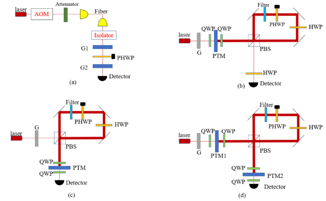
Figure 1: (Color online) (a)Schematic of weak-value-based angular-velocity measurement. A laser wave is generated by an acoustic optical modulator (AOM) and enters a polarization-dependent angular velocity measurement system consisting of two Glan prisms (G1 and G2) and the PHWP. The small angular velocity $\omega$ is induced by the PHWP and finally measured by the detector. (b): The power-recycling scheme. The PBS, which distinguishes the polarization between H and V, is combined with the PTM to reuse the failed post-selection photons repeatedly. Two QWPs near the PTM provide the initial polarization and rotate the polarization direction of cyclic light back to V. The filter in front of the PHWP refreshes the beam profile on each pass. The HWP rotates the polarization of light by $\pi/2$. (c)The signal-recycling scheme. The PTM at the output port is combined with the WWA system to form a signal-recycling cavity, thus improving the detected signal. (d)The dual-recycling scheme. Combining the power- and signal-recycling PTMs into one scheme further enhances the precision of detection. QWP: quarter-wave plate. HWP: half-wave plate. PBS: polarization-beam-splitter. PHWP: piezo-driven half-wave plate. PTM: partially transmitting mirror. H: horizontal. V: vertical.

II Standard WWA setup

We first review the standard WWA setup for angular-velocity measurement in [51]. As shown in Fig. 1(a), a non-Fourier limit Gaussian pulse $I_{0}\left(t\right)=\left(N^{2}/2\pi\tau^{2}\right)^{1/2}exp\left(-t^{2}/2\tau^{2}\right)$ , where $N$ is the number of photons and $\tau$ is the length of pulse, is sent to a polarization-dependent system. The first Glan prism(G1) combined with half-wave plate(HWP) provides the pre-selection, where the axis of G1 is vertical and the angle between G1 and HWP is $\phi_{1}$. The second Glan prism(G2), whose original orientation of axis is the horizon and rotation angle is $\phi_{2}$, provides the post-selected state. The weak interaction is expressed by a unitary operator ${\hat{U}}_{w}=exp\left(i2\omega t\hat{A}\right)$ , where $\omega$ is angular velocity by rotating HWP and $\hat{A}$ is a Hermitian operator $\hat{A}=\left|\left.L\right\rangle\right.\left\langle\left.L\right|\right.-\left|\left.R\right\rangle\right.\left\langle\left.R\right|\right.$ ($\left|\left.L\right\rangle\right.$, $\ \left|\left.R\right\rangle\right.$ are the left, right circularly polarized states). Here, we introduce a unitary operator ${\hat{U}}_{\phi}=exp\left(i2\phi_{1}\hat{A}\right)$ to represent the polarization rotation $\phi_{1}$ produced by the piezo-driven half-wave plate(PHWP). In this way, the pre-selected state of system is $\left|\left.\psi_{pre}\right\rangle\right.={\hat{U}}_{\phi}\left|\left.V\right\rangle\right.=\frac{i}{\sqrt{2}}\left[exp\left(-i2\phi_{1}\right)\left|\left.R\right\rangle-exp\left(i2\phi_{1}\right)\left|\left.L\right\rangle\right.\right.\right]$ and the post-selected state is $\left.\left|\psi_{pos}\right.\right\rangle=cos\phi_{2}\left|\left.H\right\rangle\right.-sin\phi_{2}\left.\left|V\right.\right\rangle=\frac{i}{\sqrt{2}}\left[exp\left(-i2\phi_{2}\right)\left|\left.R\right\rangle+exp\left(i2\phi_{2}\right)\left|\left.L\right\rangle\right.\right.\right]$. In this angular-velocity measurement scheme, the initial state of probe can be expressed as $\left|\left.\varphi_{0}\right\rangle\right.=\sqrt{I_{0}\left(t\right)}\left|\left.t\right\rangle\right.=\left(N^{2}/2\pi\tau^{2}\right)^{1/4}exp\left(-t^{2}/4\tau^{2}\right)\left|\left.t\right\rangle\right.$. Therefore, the intensity of detected light is given by

$$I_{d}\left(t\right) =\left|\left\langle\psi_{pos}\right|\hat{U}_{w}\left|\psi_{pre}\right\rangle\left|\left.\varphi_{0}\right\rangle\right.\right|^{2}$$ (1)

$$\approx\frac{N}{\sqrt{2\pi\tau^{2}}}{sin}^{2}\phi exp\left[-\frac{1}{2\tau^{2}}\left(t-\frac{4\omega\tau^{2}}{\phi}\right)^{2}\right],$$

where we introduce the angle $\phi=2\phi_{1}-\phi_{2}$ and assume $2\omega\tau\ll\phi\ll 1$. The corresponding weak value is given by $A_{w}=\left\langle\psi_{pos}\right|\hat{A}\left|\psi_{pre}\right\rangle/\left\langle\psi_{pos}|\psi_{pre}\right\rangle\approx-i/\phi$, which is related to the time shift. Compared with the incident light, the time shift induced by the PHWP is $\delta t=\frac{4\omega\tau^{2}}{\phi}=4\omega\tau^{2}\left|A_{w}\right|$. Based on Fisher information theory[52, 53], the Fisher information of time shift $\delta t$ is $F\left(\delta t\right)=\int{dtI_{d}\left|\frac{d}{d\delta t}lnI_{d}\right|^{2}}\approx\frac{N\phi^{2}}{\tau^{2}}$. So the minimum uncertainty of time shift detremined by Cramér-Rao bound(CRB) satisfies

$$\Delta(\delta t)=\frac{1}{\sqrt{F(\delta t)}}=\frac{\tau}{\phi\sqrt{N}}.$$ (2)

Thus, the minimum uncertainty of angular velocity is

$$\Delta\omega_{CRB}=\frac{\phi}{4\tau^{2}}\Delta\left(\delta t\right)\approx\frac{1}{4\sqrt[]{N}\tau}.$$ (3)

Therefore, the corresponding SNR is given by

$$SNR=\frac{\omega}{\left(\Delta\omega\right)}=4\omega\tau\sqrt{N}=\frac{\sqrt{N}\phi}{\tau}\delta t.$$ (4)

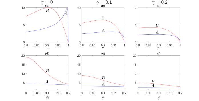
Figure 2: (Color online) Comparison of power-, signal- and dual-recycling schemes. (a), (b) and (c) correspond to the case of A and B varying with $r$ under different values of $\gamma$: 0, 0.1 and 0.2 where $\phi=0.1$. In (d), (e) and (f), we assume $r=0.9$ and plot A, B varying with $\phi$ under $\gamma=0,\ 0.1,\ 0.2$, respectively. A and B: the improvement factor of power (or signal) and dual recycling schemes. $r$: the reflection coefficient of PTM. $\gamma$: optical loss.

III Recycling technique

The methodologies of recycling techniques refer to [41] and [50], where the improvement of precision is originated from the increasing of weak-value related photons being detected. The main difference in this method is that it effectively eliminates the opposite traverse shift of the recycling profile by utilizing a filter in a manner made possible by the use of a polarization-beam-splitter (PBS). This PBS adjusts the optical path within the recycling loop, thereby mitigating the walk-off effect. In additions, the Gaussian light here is modulated in the time-domain as opposed to the traditional $x$-domain. Such arrangement induces an angular-velocity related time shift, which enables higher-precision detection. These changes distinguish this model from previous works.

III.1 Power-recycling

The power-recycled weak-value setup is shown in Fig. 1(b). The initial state $\left|\left.V\right\rangle\right.$ is provided by the Glan prism (G) and two QWPs, and we use the combination ‘HWP1 PBS HWP2’ to replace the G2 for the post-selection. The PTM, whose reflection and transmission coefficients are $r$ and $p$ $\left(r^{2}+p^{2}=1\right)$, is placed between two QWP, thus reflecting the failed post-selected light while rotating the light polarization to $\left|\left.V\right\rangle\right.$. Here we define two orthogonal states $\left|\left.\psi_{1}\right\rangle\right.$ and $\left|\left.\psi_{2}\right\rangle\right.$ to represent the input and output system states, where $\left|\left.\psi_{1}\right\rangle\ =\left|\left.V\right\rangle\right.\right.=\frac{i}{\sqrt{2}}\left(\left|\left.R\right\rangle-\left|\left.L\right\rangle\right.\right.\right)$ and $\left|\left.\psi_{2}\right\rangle\ =\left|\left.H\right\rangle\right.\right.=\frac{1}{\sqrt{2}}\left(\left|\left.R\right\rangle+\left|\left.L\right\rangle\right.\right.\right)$. Post-selected by the input and output ends, the meter states become $\left|\left.\varphi_{ref}\right\rangle\right.=\left\langle V\right|\hat{U_{w}}\hat{U_{\phi}}\left|V\right\rangle\left|\left.\varphi_{0}\right\rangle\right.$ and $\left|\left.\varphi_{out}\right\rangle\right.=\left\langle H\right|\hat{U_{w}}\hat{U_{\phi}}\left|V\right\rangle\left|\left.\varphi_{0}\right\rangle\right.$ , respectively. This produces two measurement operators $M_{11}=\left\langle\psi_{1}\right|{\hat{U}}_{w}{\hat{U}_{\phi}}\left|\psi_{1}\right\rangle=\cos{\left(\phi+2\omega t\right)}$ and $M_{12}=\left\langle\psi_{2}\right|{\hat{U}}_{w}{\hat{U}_{\phi}}\left|\psi_{1}\right\rangle=\sin{\left(\phi+2\omega t\right)}$. We introduce the non-unitary operator $\hat{L}=\sqrt{1-\gamma}$, where $\gamma$ is the single-pass power loss, to express the loss of optical imperfection in one return. Assuming the length of one traversal is $l_{cav}$, the pulse transition time of per traversal is given by $t_{cav}=2l_{cav}/c$. Generally, both the measurement operators and the meter state are related to the number of traversals $n$. For example, $M_{11}$ should be written as ${M_{11}}^{n}=\cos{\left[\phi+2\omega\left(t-nt_{cav}\right)\right]}$. [45] proved that this change is small and only induces a constant delay, which can be eliminated. Therefore, with the resonance cavity, the amplitude of the detected signal is given by the sum of amplitude from all traversal numbers,

$$\left|\left.\varphi_{p}\right\rangle\right.=pM_{12}\sum_{n=0}^{\infty}{\left(rLM_{11}\right)^{n}\left|\left.\varphi_{0}\right\rangle\right.}$$ (5)

It is a summation of the convergence series so that there is a maximum value of $n$, denoted by $n_{max}$. Therefore, the formula above can be simplified as

$$\left|\left.\varphi_{p}\right\rangle\right.=pM_{12}\sum_{n=0}^{n_{max}}{\left(rLM_{11}\right)^{n}\left|\left.\varphi_{0}\right\rangle\right.}$$ (6)

$$\approx\left(\frac{N^{2}}{2\pi\tau^{2}}\right)^{\frac{1}{4}}exp\left(-\frac{t^{2}}{4\tau^{2}}\right)\frac{p\sin{\left(\phi+2\omega t\right)}}{1-rL\cos{\left(\phi+2\omega t\right)}}|t\rangle$$

Next, we do a Taylor expansion on the function $f\left(t\right)=p\sin{\left(\phi+2\omega t\right)}/\left[1-rL\cos{\left(\phi+2\omega t\right)}\right]$ and make an approximation $f\left(t\right)\approx f\left(0\right)+tf^{\prime}\left(0\right)\approx exp\left[-f^{\prime}\left(0\right)t/f\left(0\right)\right]$. Then the amplitude of detected state is

$$\left\langle t\right.\left|\left.\varphi_{p}\right\rangle\right.\approx A\left(\frac{N^{2}}{2\pi\tau^{2}}\right)^{\frac{1}{4}}\sin^{2}{\left(\phi+2\omega t\right)}exp\left[-\frac{\left(t-\delta t_{p}\right)^{2}}{4\tau^{2}}\right]$$ (7)

where

$$A=\frac{p}{1-r\sqrt{1-\gamma}\cos{2\phi}}$$ (8)

and

$$\delta t_{p}=\frac{2\omega\tau^{2}\left(\cos{\phi}-r\sqrt{1-\gamma}\right)}{\sin{\phi}\left(1-r\sqrt{1-\gamma}\cos{2\phi}\right)}.$$ (9)

Due to the walk-off effect, the time shift changes from $\delta t$ to $\delta t_{p}$. But if placing a filter in front of the PHWP, each time being reflected by the PTM, the light pass through the filter and is projected into $\left|\left.\varphi_{0}\right\rangle\right.$. This leaves the pre-filter state as $\left|\left.\varphi\prime\right\rangle\right._{pow}=M_{11}\left|\left.\varphi_{0}\right\rangle\right./\sqrt{\left|M_{11}\left|\left.\varphi_{0}\right\rangle\right.\right|^{2}}$. Thus, the probability of surviving the filter is

$$p_{f}= \left|\left\langle\varphi_{0}\middle|\varphi\prime\right\rangle\right|^{2}=\frac{\cos^{2}{\phi}}{\sinh{4\omega^{2}\tau^{2}}+\cos^{2}{\phi}e^{-4\omega^{2}\tau^{2}}}$$ (10)

$$\approx 1-\phi^{2}\left(4\omega^{2}\tau^{2}\right)-\left(4\omega^{2}\tau^{2}\right)^{2}/2+\cdots,$$

where we make the approximation in the weak value range, $2\omega\tau\ll\phi\ll 1$. In this way, the time shift is refreshed every cycle, eliminating the walk-off effect while adding a minimum ‘filter’ loss $\gamma_{min}\approx 4\omega^{2}\tau^{2}\phi^{2}$ to the system[41]. Therefore, the power of the detected signal is given by

$$I_{pow}\approx\left(\frac{N^{2}}{2\pi\tau^{2}}\right)^{\frac{1}{2}}A^{2}\sin^{2}{\left(\phi+2\omega t\right)}exp\left[-\frac{\left(t-\delta t\right)^{2}}{2\tau^{2}}\right].$$ (11)

Similarly, the corresponding SNR determined by Cramér-Rao bound (CRB) is

$${\rm SNR}_{pow}\approx A\frac{\sqrt{N}\phi}{\tau}\delta t,$$ (12)

which is A times to the SNR of standard weak measurement.

III.2 Signal-recycling

The similar methods can be used in the signal-recycled scheme. As shown in Fig. 1(c), the optical axis of Glan prism is vertical, providing the input state $\left|\left.V\right\rangle\right.$. The post-selection is provided by the combination ‘HWP PBS QWPs’. The PTM is placed between the two QWPs to reuse the output signal. This post-selection processes provide two measurement operators: $M_{12}=\left\langle\psi_{2}\right|{\hat{U}}_{w}{\hat{U}_{\phi}}\left|\psi_{1}\right\rangle=\sin{\left(\phi+2\omega t\right)}$ and $M_{22}=\left\langle\psi_{2}\right|{\hat{U}}_{w}{\hat{U}_{\phi}}\left|\psi_{2}\right\rangle=\cos{\left(\phi+2\omega t\right)}$. In this signal-recycled cavity, the amplitude of the detected signal is given by

$$\left|\left.\varphi_{s}\right\rangle\right.=pM_{12}\sum_{n=0}^{n_{max}}{\left(rLM_{22}\right)^{n}\left|\left.\varphi_{0}\right\rangle\right.}$$ (13)

$$\approx\left(\frac{N^{2}}{2\pi\tau^{2}}\right)^{\frac{1}{4}}exp\left(-\frac{t^{2}}{4\tau^{2}}\right)\frac{p\sin{\left(\phi+2\omega t\right)}}{1-rL\cos{\left(\phi+2\omega t\right)}}|t\rangle$$

which is equivalent to $\left|\left.\varphi_{d}\right\rangle\right._{pow}$, indicating that power- and signal-recycling hold equal significance in weak-value-based power improvement. Different from previous interferometric signal-recycling schemes, the only ’clockwise’ path permits all cyclic photons to be refreshed prior to the last weak interaction. With the filter, the pre-filter state is $\left|\left.\varphi\prime\right\rangle\right._{sig}=M_{22}\left|\left.\varphi_{0}\right\rangle\right./\sqrt{\left|M_{22}\left|\left.\varphi_{0}\right\rangle\right.\right|^{2}}$, which is also equal to $\left|\left.\varphi\prime\right\rangle\right._{pow}$. Thus, the same conclusion can be obtained when considering the calculation of detected power and SNR, where $I_{sig}=I_{pow}$ and ${SNR}_{sig}={SNR}_{pow}$

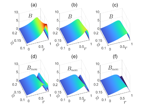
Figure 3: (Color online) Comparison of polarization-based and interferometric dual recycling schemes. (a), (b) and (c) correspond to the case of $B$ varying with $r$ and $\phi$ under different values of $\gamma$: 0, 0.1 and 0.2 in 3D, respectively. (d), (e) and (f) respresent that $B_{non}$ varies with $r$ and $\phi$ under different value of $\gamma$: 0, 0.1 and 0.2 in 3D. $B$ and $B_{non}$: the improvement factor of polarization-based and non-polarization dual recycling schemes. $r$: the reflection coefficient of PTM. $\phi$: post-selected angle. $\gamma$: optical loss.

III.3 Dual-recycling

The dual-recycled WWA scheme is shown in Fig. 1(d), where the Glan prism together with two QWPs provide the input state $\left|\left.\psi_{1}\right\rangle\ \right.$ and the output state $\left|\left.\psi_{2}\right\rangle\right.$ is provided by the combination ‘HWP PBS QWPs’. In this recycling process, all possible forms of post-selections are available so that the measurement operator of per traversal can be any of $M_{11},M_{12},M_{21},M_{22}$. Similarly, the filter in front of the PHWP projects the meter state into $\left|\left.\varphi_{0}\right\rangle\right.$, thus eliminating the walk-off effect and maintaining the large point shift associated with the WVA. This also results in a minimum optical loss $\gamma_{min}\approx 4\omega^{2}\tau^{2}\phi^{2}$, which can be ignored in the weak value range $2\omega\tau\ll\phi\ll 1$. For simple calculation, we assume the parameters of PTMs are the same and introduce the measurement matrix

$$U=\begin{bmatrix}M_{11}&M_{12}\\ M_{21}&M_{22}\\ \end{bmatrix}=\begin{bmatrix}\cos{\left(\phi+2\omega t\right)}&\sin{\left(\phi+2\omega t\right)}\\ -\sin{\left(\phi+2\omega t\right)}&\cos{\left(\phi+2\omega t\right)}\\ \end{bmatrix}$$ (14)

which is formed by four measurement operators and arranged in the order corresponding to the subscripts. $\left(U^{n}\right)_{12}$ represents the physical process that the incident light travels through the dual recycling cavity $n$ times and finally reaches the detector. Therefore, the steady state amplitude detected by the meter is given by the sum of amplitude of all traversal numbers,

$$\left\langle t\right.\left|\left.\varphi_{d}\right\rangle\right.=p\sum_{n=0}^{n_{max}}{\left(\sqrt{1-\gamma}\right)^{n+1}\left(U^{n+1}\right)_{12}p\left\langle\alpha\right.\left|\left.\varphi_{0}\right\rangle\right.}$$ (15)

$$\approx p^{2}\left(\frac{N^{2}}{2\pi\tau^{2}}\right)^{\frac{1}{4}}exp\left(-\frac{t^{2}}{4\tau^{2}}\right)\hat{L}\left(\frac{U}{I-r\sqrt{1-\gamma}U}\right)_{12}$$

$$=-\frac{p^{2}\left(\frac{N^{2}}{2\pi\tau^{2}}\right)^{\frac{1}{4}}exp\left(-\frac{t^{2}}{4\tau^{2}}\right)\sqrt{1-\gamma}\sin{\left(\phi+2\omega t\right)}}{1+\left(1-\gamma\right)r^{2}-2\sqrt{1-\gamma}rcos\left(\phi+2\omega t\right)}$$

$$\approx-\frac{p^{2}\left(\frac{N^{2}}{2\pi\tau^{2}}\right)^{\frac{1}{4}}exp\left(-\frac{t^{2}}{4\tau^{2}}\right)\sqrt{1-\gamma}\sin{\left(\phi+2\omega t\right)}}{1+\left(1-\gamma\right)r^{2}-2\sqrt{1-\gamma}r\cos{\phi}},$$

Where the last approximation is taken with the minimum ‘filter’ loss $\gamma_{min}\approx 4\omega^{2}\tau^{2}\phi^{2}$. In this way, the intensity of the detected signal is given by

$$I_{dua}\approx\left(\frac{N^{2}}{2\pi\tau^{2}}\right)^{\frac{1}{2}}B^{2}\sin^{2}{\left(\phi+2\omega t\right)}exp\left[-\frac{\left(t-\delta t\right)^{2}}{2\tau^{2}}\right]$$ (16)

where

$$B=\frac{p^{2}}{1+\left(1-\gamma\right)r^{2}-2\sqrt{1-\gamma}r\cos{\phi}}.$$ (17)

Thus, the corresponding SNR is

$${\rm SNR}_{pow}\approx B\frac{\sqrt{N}\phi}{\tau}\delta t.$$ (18)

IV Comparison

Here, we define $A$ and $B$ are the improvement factors of power(or signal) and dual recycling, respectively. It is clear that the power-, signal- and dual-recycling schemes improve the SNR of standard WWA setup $A$, $A$ and $B$ times, respectively. $A^{2}$ and $B^{2}$ also corresponds to the improvement of the detected power. Therefore, as shown in Fig. 2, we plot $A$ and $B$ varying with $r$ (Fig. 2(a), (b) and (c)) or $\phi$ (Fig. 2(d), (e) and (f)) under different values of loss $\gamma=0,\ 0.1,\ 0.2$, which correspond to ideal, low and regular loss, respectively.

As expected, the accuracy of both recycling techniques can easily exceed the corresponding standard scheme’s shot noise limit, which is proportionally scaled to 1 in Figs. 2 and 3. The similar conclusions exit in [42, 43, 44, 50]. However, we have to declare that it cannot beat the standard quantum limit since the improvement is originated from the increasing of detected photons $N\phi^{2}\to B^{2}N\phi^{2}$. Different cyclic schemes only stretch the standard quantum limit to varying degrees. In addition, both $A$ and $B$ can reach the maximum value $1/\phi=10$, as shown in Fig. 2(a), (b) and (c), where the SNR itself is amplified by the large weak value factor. However, the peak of $A$ decreases faster than that of $B$, corresponding to a larger limitation to the improvement of detecting. Therefore, the dual-recycling cavity has tolerance for a wider range of $r$ and $\gamma$, which applies to more circumstances. In Fig. 2(d), (e) and (f), we set $r=0.9$, a common parameter of the PTM, and draw the curves of $A$ and $B$ varying with $\phi$ where $\phi\in\left[0.01,\ 0.2\right]$. We can see that the improvement factor of dual recycling is larger in most weak value range, thus outperforming the power or signal recycling.

In previous dual-recycled interference-based WWA system[50], the amplification effect of pointer is reduced by the walk-off effect, leading to a limitation of the precision gain. From the equations (25) and (26) in [50], without a filter, the improvement factor $B$ changes to $B_{non}$

$$B_{non}=\xi\frac{p^{2}}{1+\left(1-\gamma\right)r^{2}-2\sqrt{1-\gamma}r\cos{\phi}},$$ (19)

where

$$\xi=\phi\frac{\cos{\phi\left[1+r^{2}\left(1-\gamma\right)\right]}-2r\sqrt{1-\gamma}}{\sin{\phi}[1+r^{2}\left(1-\gamma\right)-2r\sqrt{1-\gamma}\cos{\phi}]}.$$ (20)

Due to the proper use of the filter, a minimum filter loss replaces original performance reduction in the polarization-based dual recycling scheme. For clear comparison, in Fig. 3, we similarly set $\phi=0.1$ and plot $B$, $B_{non}$ varying with $r$ and $\phi$ under different losses. The polarization-based scheme has obvious improvement and the gaps between $B_{non}$ and $B$ decrease as the loss increases. This is established on the assumption that both systems experience the same loss $\gamma$. Actually, replacing the BS with the PBS can effectively reduce optical loss. The probability of photons surviving the PBS ($\geq 95\%$) is known to be larger than that of the BS ($\geq 90\%$). In addition, the PBS simplifies the propagation paths of cyclic photons, which reduces the crosstalk among photons. All these reasons make this polarization-based scheme advantageous in both theoretical performance and experimental application.

V Conclusion

In summary, we have proposed three polarization-based cyclic weak measurement schemes based on the angular-velocity weak measurement setup. By integrating one or two PTMs into the system to establish a resonant cavity, all incident light can be detected in principle. In our analysis, these polarization-based schemes can outperform the previous interferometric schemes due to their lower theoretical loss and improved cyclic paths. This optimized cyclic paths effectively eliminates the walk-off effect, a significant challenge in previous signal-recycling and dual-recycling schemes. Notably, among the proposed schemes, the polarization-based dual-recycling scheme demonstrates the widest optimal region.

The application of these cyclic modes are not limited to our specific experimental setup but can be extended to various weak-value-amplification realizations. This is due to the inherent presence of post-selection in all weak value setups. Additionally, leveraging quantum resources allows for precision enhancement beyond the standard quantum limit[53, 54], providing a predictable pathway towards further augmenting the performance of weak-value-based metrology.

VI acknowledgements

This work was supported by the National Natural Science Foundation of China (Grants No. 61875067).

Appendix A Optical mode matching and stability analysis

Generally, the beam will be a diffracting Gaussian beam with a waist, as opposed to the parallel beam treated above. Therefore, the waist size and positions of the incident Gaussian beam should match those of the resonance cavity itself, forming a stable self-reproduction. Here, we take the most challenging dual-recycling as an example, as illustrated in Fig. 4. Similar to the solutions of [42, 50], several well-designed lenses $L_{1},L_{2}$ and $L_{3}$ are employed to ensure the waists are located at PTM1 and PTM2.

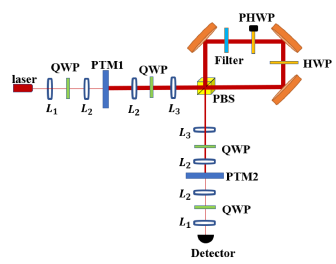
Figure 4: (Color online) Optical mode matching and cavity lengths locking. The lenses $L_{1}$, $L_{2}$ and $L_{3}$ with matched focal lengths are set on proper positions to ensure that the place of the waist and self-reproduction of Gaussian beam are at PTM1 and PTM2. QWP: quarter-wave plate. HWP: half-wave plate. PBS: polarization-beam-splitter. PHWP: piezo-driven half-wave plate. PTM: partially transmitting mirror.

The phase locking of the cavity is also essential since the ambient noise can introduce length offsets in the cavity. In Ref. [42], an error signal extracted from the output light is used to provide feedback and stabilize the power-recycling cavity using the Pound-Drever-Hall (PDH) method, which is also applicable to the signal-recycling cavity. However, when implementing the dual-recycling cavity with two different lengths, relying solely on an error signal does not provide sufficient information regarding the offsets of the PTMs. A possible approach is to adjust the post-selected angle and parameters of the PTMs such that the light reflected towards the laser is largely independent of PTM2, allowing the first PDH system to initially lock the length of PTM1 before using the second PDH system to stabilize the length of PTM2. Alternatively, a custom-designed enclosure with fixed positions for the instruments can simplify the locking operations.

References

- Aharonov et al. [1988] Y. Aharonov, D. Z. Albert, and L. Vaidman, How the result of a measurement of a component of the spin of a spin-1/2 particle can turn out to be 100, Phys. Rev. Lett. 60, 1351 (1988).
- von Neumann [2018] J. von Neumann, Mathematical Foundations of Quantum Mechanics, edited by N. A. Wheeler (Princeton University Press, Princeton, 2018).
- Steinberg [2010] A. Steinberg, A light touch, Nature 463, 890–891 (2010).
- Hardy [1992] L. Hardy, Quantum mechanics, local realistic theories, and lorentz-invariant realistic theories, Phys. Rev. Lett. 68, 2981 (1992).
- Aharonov et al. [2002] Y. Aharonov, A. Botero, S. Popescu, B. Reznik, and J. Tollaksen, Revisiting hardy’s paradox: counterfactual statements, real measurements, entanglement and weak values, Physics Letters A 301, 130 (2002).
- Lundeen and Steinberg [2009] J. S. Lundeen and A. M. Steinberg, Experimental joint weak measurement on a photon pair as a probe of hardy’s paradox, Phys. Rev. Lett. 102, 020404 (2009).
- Yokota et al. [2009] K. Yokota, T. Yamamoto, M. Koashi, and N. Imoto, Direct observation of hardy’s paradox by joint weak measurement with an entangled photon pair, New Journal of Physics 11, 033011 (2009).
- Aharonov and Vaidman [1991] Y. Aharonov and L. Vaidman, Complete description of a quantum system at a given time, Journal of Physics A: Mathematical and General 24, 2315 (1991).
- Ravon and Vaidman [2007] T. Ravon and L. Vaidman, The three-box paradox revisited, Journal of Physics A: Mathematical and Theoretical 40, 2873 (2007).
- Resch et al. [2004] K. Resch, J. Lundeen, and A. Steinberg, Experimental realization of the quantum box problem, Physics Letters A 324, 125 (2004).
- Aharonov et al. [2013] Y. Aharonov, S. Popescu, D. Rohrlich, and P. Skrzypczyk, Quantum cheshire cats, New Journal of Physics 15, 113015 (2013).
- Aharonov et al. [2021] Y. Aharonov, E. Cohen, and S. Popescu, Nature Communications 12, 4770 (2021).
- Denkmayr et al. [2014] T. Denkmayr, H. Geppert, S. Sponar, et al., Nature Communications 5, 4492 (2014).
- Duprey et al. [2018] Q. Duprey, S. Kanjilal, U. Sinha, D. Home, and A. Matzkin, The quantum cheshire cat effect: Theoretical basis and observational implications, Annals of Physics 391, 1 (2018).
- Quach [2019] J. Q. Quach, Dual to the anomalous weak-value effect of photon-polarization separation, Phys. Rev. A 100, 052117 (2019).
- Hosten and Kwiat [2008] O. Hosten and P. Kwiat, Science 319, 787 (2008).
- Zhou et al. [2012] X. Zhou, Z. Xiao, H. Luo, and S. Wen, Phys. Rev. A 85, 043809 (2012).
- Bai et al. [2020] X. Bai, Y. Liu, L. Tang, Q. Zang, J. Li, W. Lu, H. Shi, X. Sun, and Y. Lu, Opt. Express 28, 15284 (2020).
- Xu et al. [2013] X.-Y. Xu, Y. Kedem, K. Sun, L. Vaidman, C.-F. Li, and G.-C. Guo, Phys. Rev. Lett. 111, 033604 (2013).
- Li et al. [2018a] L. Li, Y. Li, Y.-L. Zhang, S. Yu, C.-Y. Lu, N.-L. Liu, J. Zhang, and J.-W. Pan, Phys. Rev. A 97, 033851 (2018a).
- Dixon et al. [2009] P. B. Dixon, D. J. Starling, A. N. Jordan, and J. C. Howell, Phys. Rev. Lett. 102, 173601 (2009).
- Viza et al. [2013] G. I. Viza, J. Martínez-Rincón, G. A. Howland, H. Frostig, I. Shomroni, B. Dayan, and J. C. Howell, Optics letters 38 16, 2949 (2013).
- Brunner and Simon [2010a] N. Brunner and C. Simon, Phys. Rev. Lett. 105, 010405 (2010a).
- Qiu et al. [2017] X. Qiu, L. Xie, X. Liu, L. Luo, Z. Li, Z. Zhang, and J. Du, Applied Physics Letters 110, 10.1063/1.4976312 (2017), 071105.
- Li et al. [2018b] H. Li, J.-Z. Huang, Y. Yu, Y. Li, C. Fang, and G. Zeng, Applied Physics Letters 112, 10.1063/1.5027117 (2018b), 231901.
- Pfeifer and Fischer [2011] M. Pfeifer and P. Fischer, Weak value amplified optical activity measurements, Opt. Express 19, 16508 (2011).
- Magaña Loaiza et al. [2014] O. S. Magaña Loaiza, M. Mirhosseini, B. Rodenburg, and R. W. Boyd, Amplification of angular rotations using weak measurements, Phys. Rev. Lett. 112, 200401 (2014).
- de Lima Bernardo et al. [2014] B. de Lima Bernardo, S. Azevedo, and A. Rosas, Ultrasmall polarization rotation measurements via weak value amplification, Physics Letters A 378, 2029 (2014).
- Qu et al. [2020] W. Qu, S. Jin, J. Sun, L. Jiang, J. Wen, and Y. Xiao, Nature Communications 11 (2020).
- Harris et al. [2017] J. Harris, R. W. Boyd, and J. S. Lundeen, Weak value amplification can outperform conventional measurement in the presence of detector saturation, Phys. Rev. Lett. 118, 070802 (2017).
- Starling et al. [2009] D. J. Starling, P. B. Dixon, A. N. Jordan, and J. C. Howell, Optimizing the signal-to-noise ratio of a beam-deflection measurement with interferometric weak values, Phys. Rev. A 80, 041803 (2009).
- Brunner and Simon [2010b] N. Brunner and C. Simon, Measuring small longitudinal phase shifts: Weak measurements or standard interferometry?, Phys. Rev. Lett. 105, 010405 (2010b).
- Feizpour et al. [2011] A. Feizpour, X. Xing, and A. M. Steinberg, Amplifying single-photon nonlinearity using weak measurements, Phys. Rev. Lett. 107, 133603 (2011).
- Kedem [2012] Y. Kedem, Using technical noise to increase the signal-to-noise ratio of measurements via imaginary weak values, Phys. Rev. A 85, 060102 (2012).
- Jordan et al. [2014] A. N. Jordan, J. Martínez-Rincón, and J. C. Howell, Technical advantages for weak-value amplification: When less is more, Phys. Rev. X 4, 011031 (2014).
- Zhang et al. [2015] L. Zhang, A. Datta, and I. A. Walmsley, Precision metrology using weak measurements, Phys. Rev. Lett. 114, 210801 (2015).
- Chen et al. [2018] G. Chen, L. Zhang, W.-H. Zhang, X.-X. Peng, L. Xu, Z.-D. Liu, X.-Y. Xu, J.-S. Tang, Y.-N. Sun, D.-Y. He, J.-S. Xu, Z.-Q. Zhou, C.-F. Li, and G.-C. Guo, Achieving heisenberg-scaling precision with projective measurement on single photons, Phys. Rev. Lett. 121, 060506 (2018).
- Liu et al. [2022] Y. Liu, L. Qin, and X.-Q. Li, Fisher information analysis on weak-value-amplification metrology using optical coherent states, Phys. Rev. A 106, 022619 (2022).
- Ferrie and Combes [2014] C. Ferrie and J. Combes, Weak value amplification is suboptimal for estimation and detection, Phys. Rev. Lett. 112, 040406 (2014).
- Knee and Gauger [2014] G. C. Knee and E. M. Gauger, When amplification with weak values fails to suppress technical noise, Phys. Rev. X 4, 011032 (2014).
- Lyons et al. [2015] K. Lyons, J. Dressel, A. N. Jordan, J. C. Howell, and P. G. Kwiat, Phys. Rev. Lett. 114, 170801 (2015).
- Wang et al. [2016] Y.-T. Wang et al., Phys. Rev. Lett. 117, 230801 (2016).
- Dressel et al. [2013] J. Dressel, K. Lyons, A. N. Jordan, T. M. Graham, and P. G. Kwiat, Phys. Rev. A 88, 023821 (2013).
- Krafczyk et al. [2021] C. Krafczyk, A. N. Jordan, M. E. Goggin, and P. G. Kwiat, Phys. Rev. Lett. 126, 220801 (2021).
- Fang et al. [2020] S.-Z. Fang, L.-L. Zhu, R.-B. Jin, H.-T. Tan, G.-X. Li, and Q.-L. Wu, Optics Communications 460, 125117 (2020).
- Meers and Strain [1991] B. J. Meers and K. A. Strain, Phys. Rev. D 43, 3117 (1991).
- Strain and Meers [1991] K. A. Strain and B. J. Meers, Phys. Rev. Lett. 66, 1391 (1991).
- Abbott et al. [2016a] B. P. Abbott et al. (LIGO Scientific Collaboration and Virgo Collaboration), Phys. Rev. Lett. 116, 061102 (2016a).
- Abbott et al. [2016b] B. P. Abbott et al. (LIGO Scientific Collaboration and Virgo Collaboration), Phys. Rev. Lett. 116, 131103 (2016b).
- Zhong et al. [2023] Z.-R. Zhong, W.-J. Tan, Y. Chen, and Q.-L. Wu, Dual-recycled interference-based weak value metrology, Phys. Rev. A 108, 032608 (2023).
- Fang et al. [2021] S.-Z. Fang, H.-T. Tan, G.-X. Li, and Q.-L. Wu, Weak value amplification for angular velocity measurements, Appl. Opt. 60, 4335 (2021).
- Care [1983] C. M. Care, Probabilistic and statistical aspects of quantum theory: North-holland series in statistics and probability vol 1, Physics Bulletin 34, 395 (1983).
- Pang et al. [2014] S. Pang, J. Dressel, and T. A. Brun, Entanglement-assisted weak value amplification, Phys. Rev. Lett. 113, 030401 (2014).
- Chen et al. [2019] J.-S. Chen, B.-H. Liu, M.-J. Hu, X.-M. Hu, C.-F. Li, G.-C. Guo, and Y.-S. Zhang, Realization of entanglement-assisted weak-value amplification in a photonic system, Phys. Rev. A 99, 032120 (2019).
- Helstrom and Kennedy [1974] C. Helstrom and R. Kennedy, Noncommuting observables in quantum detection and estimation theory, IEEE Transactions on Information Theory 20, 16 (1974).