Preconditioning for time-harmonic Maxwell’s equations using the Laguerre transform

Abstract

A method of numerically solving Maxwell’s equations is considered for modeling harmonic electromagnetic fields. The vector finite element method makes it possible to obtain a physically consistent discretization of the differential equations. However, solving large systems of linear algebraic equations with indefinite ill-conditioned matrices is a challenge. The high order of the matrices limits the capabilities of the Gaussian method to solve such systems, since this requires large RAM and much calculation. To reduce these requirements, an iterative preconditioned algorithm based on integral Laguerre transform in time is used. This approach allows using multigrid algorithms and, as a result, needs less RAM compared to the direct methods of solving systems of linear algebraic equations.

1 Introduction

Solving Maxwell’s equations is one of the major problems of mathematical modeling. Of particular interest is calculating harmonic electromagnetic fields in geometrically complex domains. In this case, as a rule, the vector finite element method with basis functions from the Nedelec functional space is used [1, 2]. The thus obtained discrete problem gives a physically correct approximation of Maxwell’s equations providing, in a natural way, the discontinuity of normal components and the continuity of tangential components of the electromagnetic field without adding fictitious resonance frequencies to the spectrum.

Let $\Omega\subset\mathbb{R}^{d},\ d=2\text{ or }3$ be a bounded Lipschitz domain with two disjoint connected boundaries $\Gamma$ and $S$ with outward unit normal $\mathbf{n}$. By solving the time-harmonic Maxwell equations under perfect conducting boundary conditions on $S$ and impedance conditions on $\Gamma$:

$$\nabla\times\left(\mu_{r}^{-1}\times\nabla\tilde{\textbf{E}}\right)+\kappa^{2}\epsilon_{r}\tilde{\textbf{E}}=\tilde{\textbf{F}}\;\text{in}\;\Omega,$$ (1a)

$$\textbf{n}\times\tilde{\textbf{E}}=0\;\text{on}\;S,$$ (1b)

$$\mu_{r}^{-1}\left(\nabla\times\tilde{\textbf{E}}\right)\times\textbf{n}-\mathrm{i}\kappa\lambda\left(\textbf{n}\times\tilde{\textbf{E}}\right)\times\textbf{n}=0\;\text{on}\;\Gamma,$$ (1c)

we can get a time-harmonic electric field $\tilde{\textbf{E}}:\Omega\rightarrow\mathbb{R}^{d}$ corresponding to a given current density $\tilde{\mathbf{F}}\in L_{2}(\mathbb{R})^{d}$ which is related to the wave number $\kappa=\omega\sqrt{\epsilon_{r}(\mathbf{x})\mu_{r}(\mathbf{x})}$ and frequency $\omega$. The relative permittivity and permeability are defined by

$$\epsilon_{r}=\frac{1}{\epsilon_{0}}\left(\epsilon(\mathbf{x})+\frac{i\sigma(\mathbf{x})}{\omega}\right),\quad\mu_{r}=\frac{\mu(\mathbf{x})}{\mu_{0}},$$

where $\epsilon,\mu$ are the electric and magnetic permeability (for a vacuum $\epsilon_{0},\mu_{0}$), $\sigma$ is the conductivity, $\lambda$ is the impedance coefficient.

The Hilbert spaces corresponding to the Maxwell equation are defined by

$$H\left(\mathrm{curl};\Omega\right)=\left\{\textbf{u}\in\left(L_{2}\left(\Omega\right)\right)^{d}:\nabla\times\textbf{u}\in\left(L_{2}\left(\Omega\right)\right)^{d}\right\},$$

$$H_{0}=\left\{\textbf{u}\in H\left(\mathrm{curl};\Omega\right):\textbf{n}\times\textbf{u}\left|{}_{\Gamma}\right.\in\left(L_{2}\left(\Gamma\right)\right)^{d},\textbf{n}\times\textbf{u}=0\;\text{on}\;S\right\},$$

equipped with the following curl norms:

$$\|\textbf{u}\|_{H\left(\mathrm{curl};\Omega\right)}^{2}={\|\textbf{u}\|^{2}_{\left(L_{2}\left(\Omega\right)\right)^{d}}+\|\nabla\times\textbf{u}\|^{2}_{\left(L_{2}\left(\Omega\right)\right)^{d}}},$$

$$\|\textbf{u}\|^{2}_{H_{0}}={\|\textbf{u}\|^{2}_{H\left(\mathrm{curl};\Omega\right)^{d}}+\|\textbf{n}\times\textbf{u}\|^{2}_{\left(L_{2}\left(\Gamma\right)\right)^{d}}}.$$

To simplify the notation, we introduced the following abbreviations for inner products and boundary integrals:

$$\left(\mathbf{u},\mathbf{{v}}\right)_{\Omega}=\int_{\Omega}\mathbf{u}\cdot{\mathbf{\bar{v}}}d\Omega,\quad\left<\mathbf{u},\mathbf{{v}}\right>_{\Gamma}=\int_{\Gamma}\mathbf{u}\cdot{\mathbf{\bar{v}}}d\Gamma,$$

where the overbar denotes complex conjugation. Using the Galerkin method, we arrive at the variational problem of finding $\tilde{\textbf{E}}\in H_{0}$ such that

$$\left(\mu_{r}^{-1}\nabla\times\tilde{\textbf{E}},\nabla\times\mathbf{v}\right)_{\Omega}-\kappa^{2}\epsilon_{r}\left(\tilde{\textbf{E}},\mathbf{v}\right)_{\Omega}-\mathrm{i}\kappa\lambda\left<\tilde{\textbf{E}}_{T},\mathbf{v}_{T}\right>_{\Gamma}=\left(\tilde{\mathbf{F}},{\mathbf{v}}\right)_{\Omega},\quad\forall\;{\mathbf{v}}\in{H_{0}}.$$ (2)

If the calculation domain $\Omega$ is approximated, for example, by a triangular $(d=2)$ or tetrahedral $(d=3)$ grid, and the space $H_{0}$ is approximated by a finite-dimensional Nedelec subspace $H_{0}^{h}\in H_{0}$ [3], the solution of the variation problem (2) can be obtained by solving the system of linear algebraic equations

$$A\mathbf{X}=\mathbf{Y},\quad A\in\mathbb{C}^{n\times n},\quad\mathbf{X},\mathbf{Y}\in\mathbb{C}^{n}.$$ (3)

Significant computational difficulties arise when solving an ill-conditioned system of linear algebraic equations (SLAE) of the form (3). Although many computational methods of linear algebra have been developed for this purpose, the problem of solving high-order indefinite SLAEs has not yet been fully solved, especially with iterative methods [4]. In engineering calculations, preference is given to direct algorithms of solving SLAEs with various variants of the Gaussian method [5], which is due to the fact that they are computationally reliable, but fast convergence of iterative methods is not guaranteed. However, the direct methods require great numbers of arithmetic operations, large RAM, and use of multiprocessor computing systems even for solving relatively small problems.

An alternative to direct methods is iterative algorithms [6] which, for many problems of mathematical modeling, make it possible to obtain SLAE solutions with less numbers of arithmetic operations. For the vector Helmholtz equation with a sign-definite operator, various approaches have been developed, which are mainly based on algebraic multigrid methods [7, 8, 9, 10]. In some particular cases, multi-grid methods can be used to solve sign-indefinite problems [11]. A geometric multigrid method can be used when it is possible to construct a sequence of nested calculation grids [12], which is difficult in geometrically complex domains.

In the general case, the difficulty in solving the ill-conditioned system of equations (3) is that the principal part of (1a) has a nontrivial null-space, since $\nabla\times\left(\mu_{r}^{-1}\nabla\times\left(\nabla\psi\right)\right)=0$ for any three times differentiable scalar function $\psi$. Here the dimensionality of the zero subspace is proportional to the number of grid nodes [13], which does not allow using iterative algorithms for solving the SLAEs efficiently. The sign-indefiniteness and the presence of a nontrivial zero kernel of the matrix of a SLAE do not prevent the use of iterative methods; however, their combination when solving Maxwell’s equations greatly reduces the convergence rate.

To relax the requirements for computing resources, alternative approaches based on the principle of maximum amplitude have been developed [14, 15]. For example, for the scalar Helmholtz equation

$$\Delta\tilde{u}(\textbf{x})+k^{2}\tilde{u}(\textbf{x})=-\tilde{f}(\textbf{x}),\quad k^{2}=\frac{\omega^{2}}{v^{2}},\quad\mathbf{x}\in\mathbb{R}^{d},\;d=2\text{ or }3,$$ (4)

where $k^{2}$ is the squared wave vector modulus, $\omega$ is the cyclic frequency, and $v$ is the wave propagation speed in the medium. The solution to equation (4) is understood as the limit

$$\tilde{u}(\textbf{x})=\lim\limits_{t\to 0}u(\textbf{x},t)e^{\mp\mathrm{i}\omega t},\quad\mathrm{i}=\sqrt{-1}.$$ (5)

Here the function $u(\textbf{x},t)$ is a solution to the following Cauchy problem:

$$\begin{array}[]{l}\Delta u(\textbf{x})-\frac{1}{v^{2}}\partial^{2}_{tt}u(\textbf{x})=-\tilde{f}(\textbf{x})e^{\pm\mathrm{i}\omega t},\\ \\ u(\textbf{x},0)=\partial_{t}u(\textbf{x},0)=0.\end{array}$$ (6)

Along with the limiting absorption principle or the Sommerfeld radiation conditions [16], the limiting amplitude principle makes it possible to identify the unique solution that is physically correct. A necessary condition of correctness of the representation (5) is that the function $\tilde{f}(\mathbf{x})$ must be orthogonal to all eigenfunctions of the steady problem (4). Hence, for bounded areas the limiting amplitude principle is not valid. From the computational point of view, no need to solve ill-conditioned sign-indefinite SLAEs is an advantage of this class of methods. A shortcoming is that, due to the low convergence rate, which depends on the model parameters and the dimensions of the calculation domain, it may be necessary to calculate a significant number of wave field periods in order to achieve a given accuracy by means of ”pseudo transient” computations.

In order to reduce the computational costs, some advanced approaches known as ”controllability methods” have been proposed. They require multiple solutions of Maxwell’s equations in time to minimize a penalty functional [17, 18, 19], whose minimum is reached on a solution that is close to that of equation (1). In contrast to the limiting amplitude principle, the use of the additional functional reduces the number of problems to be solved in time; however, the thus obtained solution should be understood in a very weak sense. The main difficulty of this class of methods is that a solution to the functional may be nonunique. In addition, there is no guarantee that the solution providing a minimum to the functional will be close to the solution of the problem (1). Papers [20, 21] consider various wave field filtering procedures to identify the unique solution obtained in this way.

When calculating a large number of wavefield periods, small grid steps in space and time must be used to ensure sufficient accuracy. For explicit schemes, the integration time step is limited by the Courant stability condition [22]. Implicit schemes allow calculations with larger time steps. This may cause parasitic non-physical oscillations in the wave field, and makes it necessary to solve sign-indefinite SLAEs.

The present study deals with preconditioning of a SLAE of the form (3). We construct a preconditioning operator based on repeatedly solving Maxwell’s equations in time using Laguerre transform. This makes it possible to obtain a series of problems with a sign-definite operator, for which the discrete problem can be effectively solved by multigrid algorithms. The use of Laguerre transform eliminates numerical dispersion in time, and there is no need to perform calculations with very fine time resolution. In contrast to ”controllability methods” and other similar approaches, solving the problem (3) directly does not require any additional auxiliary functionals, which makes it easier to analyze the accuracy of the results.

2 Laguerre based preconditioner

Consider integral Laguerre transform in time for preconditioning of SLAE (3). This transform has been used to solve direct and inverse problems in modeling of seismic and electromagnetic wave fields [23, 24, 25, 26, 27]. It has been shown that with this approach no sign-indefinite SLAEs need be solved and spectral accuracy in approximating the time derivative is provided. Also, Laguerre transform makes it possible to stabilize unstable difference schemes when solving problems of wave field continuation from the surface into depth [28, 29]

2.1 Laguerre transform

Consider Laguerre functions [30], which are defined as

$$l_{m}(t)=e^{-t/2}\mathsf{L}_{m}(t),\quad t\geq 0,\;m=0,1,2...,$$

where $\mathsf{L}_{m}(t)$ is the Laguerre polynomial of degree $m$, which is defined by the Rodrigues formula

$$\mathsf{L}_{m}(t)=\frac{e^{t}}{m!}\frac{d^{m}}{dt^{m}}\left(t^{m}e^{-t}\right)=\frac{1}{m!}\left(\frac{d}{dt}-1\right)^{m}t^{m}.$$

We will use $L_{2}[0,\infty)$ to denote the space of square integrable functions $f:[0,\infty)\rightarrow\mathbb{R}$

$$L_{2}[0,\infty)=\left\{f:\int_{0}^{\infty}|f(t)|^{2}dt<\infty\right\}.$$

The Laguerre functions are a complete orthonormal system in $L_{2}[0,\infty)$

$$\int_{0}^{\infty}l_{m}(t)l_{n}(t)dt=\left\{\begin{array}[]{ll}0,&m\neq n,\\ 1,&m=n.\end{array}\right.$$

This guarantees that for any function $f(t)\in L_{2}[0,\infty)$ there is a Laguerre expansion

$$f(t)\sim\eta\sum_{m=0}^{\infty}\bar{a}_{m}l_{m}(\eta t),\quad\bar{a}_{m}=\int_{0}^{\infty}f(t)l_{m}(\eta t)dt,\quad t\geq 0,$$ (7)

where $\eta>0$ is a scaling parameter for the Laguerre functions to increase the convergence rate of the series [31].

Let us consider bilateral Laguerre transform for functions $g(t)\in L_{2}(\mathbb{R})$ [32]:

$$\begin{array}[]{ll}\displaystyle g(t)\sim\eta\sum_{m=-\infty}^{+\infty}\bar{b}_{m}\phi_{m}(\eta t),\quad\bar{b}_{m}=\int_{-\infty}^{+\infty}g(t)\phi_{m}(\eta t)dt,\end{array}$$ (8)

where $\phi_{m}(t)$ are functions that are orthonormal on the entire real axis and defined as follows:

$$\phi_{m}(t)=\left\{\begin{array}[]{lc}\left.\begin{array}[]{ll}l_{m}(t),&t\geq 0\\ 0,&t<0\end{array}\right\}\quad m=0,1,2,...\quad,\\ \left.\begin{array}[]{ll}-l_{-m-1}(-t),&t<0\\ 0,&t\geq 0\end{array}\right\}\quad m=-1,-2,...\quad.\end{array}\right.$$ (9)

Then Plancherel’s extension of the Fourier transform for the function $\phi_{m}(t)$ has the form [33]:

$$\tilde{\phi}_{m}(\omega)=\mathcal{F}\{\phi_{m}(\eta t)\}=\frac{1}{2\pi}\int_{-\infty}^{+\infty}\phi_{m}(\eta t)e^{-\mathrm{i}\omega t}dt=\frac{\eta}{2\pi}\frac{\left(\mathrm{i}\omega-\eta/2\right)^{m}}{\left(\mathrm{i}\omega+\eta/2\right)^{m+1}},\quad m\in\mathbb{Z}.$$ (10)

Hence, the Fourier transform is expressed in terms of the Laguerre series coefficients as follows:

$$\tilde{g}(\omega)=\mathcal{F}\{g(t)\}\sim\frac{\eta}{2\pi}\sum_{m=-\infty}^{+\infty}\bar{b}_{m}\tilde{\phi}_{m}(\omega).$$ (11)

This relation will be used to construct a preconditioning procedure for solving SLAEs of the form (3). The calculation time can be decreased by adjusting the number of terms in the Laguerre series expansion, since for preconditioning the solution is allowed to be calculated approximately.

2.2 The Laguerre transform for Maxwell’s equation

Taking into account the operator properties of Fourier transform $i\omega\leftrightarrow\partial_{t}$ and $-\omega^{2}\leftrightarrow\partial_{tt}$, we can write the problem (1) in time as follows:

$$\begin{array}[]{rl}\nabla\times\left(\mu_{r}^{-1}\times\nabla\textbf{E}\right)+\frac{\mu_{r}}{\epsilon_{0}}\left(\epsilon\partial_{tt}-\partial_{t}\sigma\right)\textbf{E}=\mathbf{F}&\text{in}\;\Omega,\\ \textbf{n}\times\textbf{E}=0&\text{on}\;S,\\ \mu_{r}^{-1}\left(\nabla\times{\textbf{E}}\right)\times\textbf{n}-\lambda\sqrt{\mu_{r}\epsilon_{r}}\partial_{t}\left(\textbf{n}\times{\textbf{E}}\right)\times\textbf{n}=0&\text{on}\;\Gamma.\end{array}$$ (12)

A solution to equation (12) will be sought for in the form of a series of Laguerre functions:

$$\mathbf{E}(\mathbf{x},t)\approx\eta\sum_{m=0}^{M-1}\mathbf{\bar{E}}_{m}l_{m}(\eta t),$$ (13)

where the number of expansion coefficients is chosen according to the required accuracy of approximation of the solution on an interval, $t\in[0,t_{1}]$. Taking into account $f(0)=f^{\prime}(t)=0$ and assuming $\lim_{t\rightarrow\infty}f(t)=\lim_{t\rightarrow\infty}f^{\prime}(t)=0$, one can show [34] that

$$\int_{0}^{\infty}\frac{d^{k}f(t)}{dt^{k}}l_{m}(\eta t)dt=\left(\frac{\eta}{2}\right)^{k}\bar{f}^{m}+\Phi_{k}(\bar{f}^{m}),\quad m=0,1,2...,$$ (14)

where for $k=1,2$ we have

$$\Phi_{1}(\bar{f}^{m})\equiv\eta\sum_{k=0}^{m-1}\bar{f}^{k},\quad\Phi_{2}(\bar{f}^{m})\equiv\eta^{2}\sum_{k=0}^{m-1}(m-k)\bar{f}^{k},\quad m=0,1,2....$$

Then, assuming $\textbf{E}|_{t=0}=\partial_{t}\textbf{E}|_{t=0}=\lim_{t\rightarrow\infty}\mathbf{E}(t)=\lim_{t\rightarrow\infty}\partial_{t}\mathbf{E}(t)=0$ and applying the Laguerre transform to the system (12), taking into account the properties (14), we obtain

$$\begin{array}[]{rl}\nabla\times\left(\mu_{r}^{-1}\times\nabla\bar{\mathbf{E}}_{m}\right)+\beta_{1}\bar{\mathbf{E}}_{m}=\mathbf{\bar{F}}_{m}+\sigma\mu_{r}/\epsilon_{0}\Phi_{1}(\bar{\mathbf{E}}_{m})+\mu_{r}\epsilon_{r}\Phi_{2}(\bar{\mathbf{E}}_{m})&\text{in}\;\Omega,\\ \mathbf{n}\times\bar{\textbf{E}}_{m}=0&\text{on}\;S,\\ \mu_{r}^{-1}\left(\nabla\times{\mathbf{\bar{E}}}_{m}\right)\times\mathbf{n}-\beta_{2}\left(\mathbf{n}\times{\mathbf{\bar{E}}_{m}}\right)\times\mathbf{n}=\lambda\sqrt{\mu_{r}\epsilon_{r}}\Phi_{1}\left(\left(\mathbf{n}\times{\mathbf{\bar{E}}_{m}}\right)\times\mathbf{n}\right)&\text{on}\;\Gamma,\end{array}$$ (15)

where $\beta_{1}=\frac{\mu_{r}}{4\epsilon_{0}}\left(\epsilon\eta^{2}-2\eta\sigma\right)$, $\beta_{2}=\frac{\eta}{2}\lambda\sqrt{\mu_{r}\epsilon_{r}}$.

To calculate the expansion coefficients of the series (13), we approximate the problem (15) by using a vector finite element method for the same subspace $H^{h}_{0}$ and the grid as in the problem (1):

$$\left(\mu_{r}^{-1}\nabla\times\bar{\textbf{E}}_{m},\nabla\times\mathbf{v}\right)_{\Omega}-\beta_{1}\left(\bar{\textbf{E}}_{m},\mathbf{v}\right)_{\Omega}-\beta_{2}\left<\bar{\textbf{E}}_{T,m},\mathbf{v}_{T}\right>_{\Gamma}=\left(\bar{\mathbf{Q}}_{m},{\mathbf{v}}\right)_{\Omega},\quad\forall\;{\mathbf{v}}\in{H_{0}}.$$ (16)

Then the following SLAE is solved several times with the same matrix and different right-hand sides:

$$B\mathbf{\bar{E}}_{m}=\mathbf{\bar{G}}_{m-1}+\mathbf{\bar{F}}_{m},\quad B\in\mathbb{R}^{n\times n},\quad\mathbf{\bar{E}}_{m},\mathbf{\bar{G}}_{m-1},\mathbf{\bar{F}}_{m}\in\mathbb{R}^{n}$$ (17)

where the vector $\mathbf{\bar{G}}_{m-1}$ is a linear combination of $\mathbf{\bar{E}}_{k}$, $k=0,1,2,...,m-1$ and $\mathbf{\bar{E}}_{-1}\equiv 0$. At $\beta_{1}>0$ (i.e. $\eta>\frac{2\sigma}{\epsilon}$), this sign-definite SLAE can be effectively solved by an algebraic multigrid algorithm [10]. Compared to direct methods for solving SLAEs, multigrid methods need much less RAM.

3 Choosing the right-hand side

Consider how to choose the right-hand side for the problem (16),(17) to precondition SLAE (3). Since the functions $\sin(\omega t),\cos(\omega t)$ do not belong to the space $L_{2}[0,\infty]$, the Laguerre series will diverge for the right-hand sides of the form $\mathbf{F}(\mathbf{x},t)=\mathbf{\tilde{F}}(\textbf{x})e^{i\omega t}$. However, convergence can be achieved if the right-hand side is multiplied by a function defining a rectangular window:

$$\Pi\left(t\right)=\left\{\begin{array}[]{lr}1,&|t|\leq\tau\\ 0,&elsewhere.\end{array}\right.$$

Hence,

$$\mathbf{F}(\mathbf{x},t)=\mathbf{\tilde{F}}(\textbf{x})e^{i\omega t}\Pi\left({t-\tau}\right).$$

Then the harmonic electromagnetic field will be approximately calculated as follows:

$$\mathbf{\tilde{E}}(\mathbf{x},\omega)\approx\frac{\eta}{2}\sum_{m=0}^{M}\mathbf{\bar{E}}_{m}(\mathbf{x})\tilde{\phi}_{m}(\omega).$$ (18)

Since the function $\Pi(t)$ is not differentiable, the Laguerre series (7) will be slowly converging. On the other hand, as the duration of the signal decreases with time, the width of its spectrum increases, since after a harmonic source is multiplied by the function $\Pi(t)$ the spectrum is the convolution of the delta function with a $sinc$ function, which causes the Gibbs effect. Also, the ”spectrum leakage” effect makes it a smooth function of $\omega$, which increases the convergence rate of the series (18). Thus, one cannot provide equally fast convergence of the Laguerre series to approximate the source in the time domain and to approximate the electromagnetic field in the spectral domain.

Window functions such as Kaiser, Hanning, and Chebyshev ones have been additionally tested. However, at this stage of the study their use does not provide the convergence of the iterative process for solving the SLAE. This can be explained by the fact that the best means for retaining such characteristics as variance compensation, dispersion factors, total energy, and coherent gain is a rectangular window [35], which turned out to be important in preconditioning.

4 Numerical experiments

Consider solving equation (1) for the two media models shown in Figures 1a and 3a. The parameters of the medium are as follows: permeability $\mu_{1}=30$, $\mu_{2}=5$, permittivity $\epsilon_{r}=1$. A point source with frequency $\omega=2\pi/100$ is located at the center of the calculation domain $\Omega$. After a finite-element approximation of the variational problem (2) with second-order Nedelec’s elements, we solve a SLAE of the form (3), for which we use the GMRES($k$) method [36, 37] and the preconditioning procedure (13), (17) with the Laguerre transform parameter $\eta=75$ and time window duration $\tau=4\pi/\omega$. The coefficients $\bar{\mathbf{E}}_{m}$ of the series (11) will be calculated with accuracy $\varepsilon_{lag}=10^{-5}$. As has been shown by computational experiments, to solve the problem (17) we need only a few iterations of the conjugate gradient method with a multigrid preconditioner called the Auxiliary-space Maxwell Solver [10].

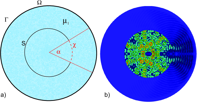
(a)

Figure 1: a) Homogeneous model of medium with internal PEC boundary $S$, b) wave field magnitude for a source located at the center of the calculation domain

Let us investigate the convergence of the GMRES($k$) method, $k=100$, without preconditioning. The wave field magnitude for the first and second models is shown in Figs. 1b and 3b, respectively. As can be seen in Fig. 2a, the convergence rate depends on the length $\chi(\alpha)$ of the segment PEC of the boundary $S$. If the boundary $S$ is absent ($\alpha=2\pi$) and there are no reflected waves, the iterative process converges very fast. If the boundary is almost closed or completely closed ($\alpha\leq 0.05\pi$), the GMRES($k$) method stagnates.

For the heterogeneous model stagnation is observed (Fig. 4a) already at $\alpha=0.05\pi$, although for the homogeneous model with the same segment length $\chi(\alpha)$ the iterative process converges. Thus, without preconditioning the iterative methods converge very slowly for heterogeneous models, in particular for PEC boundary conditions resulting in multiple internal reflections. By contrast, the GMRES ($k$) method with a preconditioner of the form (13), (17) provides convergence for both the homogeneous model and the heterogeneous one. As the slot length $\chi(\alpha)$ decreases, there appear multiple reflections of waves from the boundary $S$; and the waves need more time to leave the calculation domain $\Omega$. As a consequence, the convergence rate for small values of $\alpha$ decreases, since the preconditioning operator approximates the solution in some time interval $[0,\tau]$, which does not guarantee that the solution of the problem (17) is close to that of the problem (3).

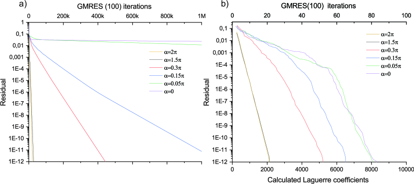
Figure 2: Residual for the GMRES($k$) method versus the number of iterations for the homogeneous model (Fig. 1a): a) without preconditioning and b) with preconditioning

Figure 3: a) Heterogeneous model of the medium with internal PEC boundary $S$, b) wavefield magnitude for a source with frequency $2\pi/100$ located at the center of the calculation domain

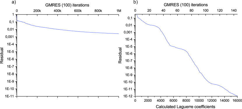
Figure 4: Residual for the GMRES($k$) method versus the number of iterations for the heterogeneous model (Fig. 3a): a) without preconditioning and b) with preconditioning

5 Conclusions

This paper considered solving Maxwell’s equations in the frequency domain. The sign-indefiniteness, poor conditioning of the SLAE, and the presence of a nontrivial zero subspace make it difficult to reach high convergence rates of iterative methods when considering many engineering problems. The algorithms based on the Gaussian method require a significant number of arithmetic operations, as well as large RAM, even in solving relatively small problems. The main requirement in the development of the present approach was to decrease the minimum RAM needed. For this, a preconditioning procedure was proposed, which is based on integral Laguerre transform in time. This makes it possible to obtain a sign-definite SLAE, which can be solved by multigrid methods that do not require large RAM.

In the two-dimensional case the approach is not efficient, since it needs more calculation time than the direct methods. However, in the three-dimensional case the efficiency will be much better, since the RAM required is several orders of magnitude less than that of the direct methods. The calculation time will also decrease, since the computational complexity of multigrid methods is less than that of direct algorithms. Also note that the computational procedure under consideration does not stagnate, which is due to the filtration properties of the Laguerre transform which were used to suppress the unstable solution components in our previous studies.

References

- [1] J.C. Nédélec. Mixed finite elements in . Numerische Mathematik, 35(3):315–341, 1980.
- [2] J.C. Nédélec. A new family of mixed finite elements in . Numerische Mathematik, 50:57–81, 1986.
- [3] P. Monk. An analysis of nédélec's method for the spatial discretization of maxwell's equations. Journal of Computational and Applied Mathematics, 47(1):101–121, June 1993.
- [4] O. G. Ernst and M. J. Gander. Why it is Difficult to Solve Helmholtz Problems with Classical Iterative Methods, pages 325–363. Springer Berlin Heidelberg, Berlin, Heidelberg, 2012.
- [5] I.S. Duff, A.M. Erisman, and J.K. Reid. Direct Methods for Sparse Matrices. Oxford University Press, January 2017.
- [6] H. A. van der Vorst. Iterative Krylov Methods for Large Linear Systems, volume 13. Cambridge University Press, 2003.
- [7] R. Hiptmair. Multigrid method for maxwell's equations. SIAM Journal on Numerical Analysis, 36(1):204–225, January 1998.
- [8] J. Jones and B. Lee. A multigrid method for variable coefficient maxwell's equations. SIAM Journal on Scientific Computing, 27(5):1689–1708, January 2006.
- [9] R. Hiptmair and J. Xu. Nodal auxiliary space preconditioning in h(curl) and h(div) spaces. SIAM Journal on Numerical Analysis, 45(6):2483–2509, January 2007.
- [10] T.V. Kolev and P.S. Vassilevski. Parallel auxiliary space AMG for h(curl) problems. Journal of Computational Mathematics, 27(5):604–623, June 2009.
- [11] O.V. Nechaev, E.P. Shurina, and M.A. Botchev. Multilevel iterative solvers for the edge finite element solution of the 3d maxwell equation. Computers & Mathematics with Applications, 55(10):2346–2362, 2008. Advanced Numerical Algorithms for Large-Scale Computations.
- [12] D.N. Arnold, R.S. Falk, and R. Winther. Multigrid in h (div) and h (curl). Numerische Mathematik, 85(2):197–217, April 2000.
- [13] L. Xue and D. Jiao. Method for analytically finding the nullspace of stiffness matrix for both zeroth-order and higher order curl-conforming vector bases in unstructured meshes. IEEE Transactions on Microwave Theory and Techniques, 68(2):456–468, 2020.
- [14] A.N. Tikhonov and A.A. Samarskii. On the radiation principle. Zh. Eksper. i Teoret. Fiz., 18(2):243–248, 1948.
- [15] A.N. Tikhonov and A.A. Samarskii. Equations of Mathematical Physics. Dover Publications, 1990.
- [16] A. Sommerfeld. Die greensche funktion der schwingungslgleichung. Jahresbericht der Deutschen Mathematiker-Vereinigung, 21:309–352, 1912.
- [17] M.O. Bristeau, R. Glowinski, and J. Périaux. Controllability methods for the computation of time-periodic solutions: Application to scattering. Journal of Computational Physics, 147(2):265–292, December 1998.
- [18] M.J. Grote and J. H. Tang. On controllability methods for the helmholtz equation. Journal of Computational and Applied Mathematics, 358:306–326, October 2019.
- [19] T. Chaumont-Frelet, M.J. Grote, S. Lanteri, and J.H. Tang. A controllability method for maxwell's equations. SIAM Journal on Scientific Computing, 44(6):A3700–A3727, December 2022.
- [20] D. Appelö, F. Garcia, and O. Runborg. WaveHoltz: Iterative solution of the helmholtz equation via the wave equation. SIAM Journal on Scientific Computing, 42(4):A1950–A1983, January 2020.
- [21] Z. Peng and D. Appelo. EM-WaveHoltz: A flexible frequency-domain method built from time-domain solvers. IEEE Transactions on Antennas and Propagation, 70(7):5659–5671, July 2022.
- [22] R. Courant, K. Friedrichs, and H. Lewy. Über die partiellen differenzengleichungen der mathematischen physik. Mathematische Annalen, 100:32–74, 1928.
- [23] B. G. Mikhailenko and A. F. Mastryukov. Numerical solution of maxwell’s equations for anisotropic media using the laguerre transform. Russian Geology and Geophysics, 49:621–627, 2008.
- [24] A.F. Mastryukov. Solving an inverse problem for maxwell’s equations numerically with laguerre functions. Numerical Analysis and Applications, 6(4):279–288, October 2013.
- [25] A. G. Fatyanov and A. V. Terekhov. High-performance modeling acoustic and elastic waves using the parallel dichotomy algorithm. J. Comp. Phys., 230(5):1992–2003, 2011.
- [26] A. V. Terekhov. Spectral-difference parallel algorithm for the seismic forward modeling in the presence of complex topography. Journal of Applied Geophysics, 115(0):206–219, 2015.
- [27] B. G. Mikhailenko. Spectral Laguerre method for the approximate solution of time dependent problems. Applied Mathematics Letters, 12:105–110, 1999.
- [28] A. V. Terekhov. The Laguerre finite difference one-way equation solver. Computer Physics Communications, 214:71 – 82, 2017.
- [29] A. V. Terekhov. The stabilization of high-order multistep schemes for the Laguerre one-way wave equation solver. Journal of Computational Physics, 368:115 – 130, 2018.
- [30] NIST Digital Library of Mathematical Functions. http://dlmf.nist.gov/, Release 1.1.2 of 2021-06-15. F. W. J. Olver, A. B. Olde Daalhuis, D. W. Lozier, B. I. Schneider, R. F. Boisvert, C. W. Clark, B. R. Miller, B. V. Saunders, H. S. Cohl, and M. A. McClain, eds.
- [31] William T. Weeks. Numerical inversion of Laplace transforms using Laguerre functions. J. ACM, 13(3):419–429, July 1966.
- [32] J. Keilson, W. Nunn, and U. Sumita. The bilateral Laguerre transform. Applied Mathematics and Computation, 8(2):137 – 174, 1981.
- [33] H. Weber. Numerical computation of the Fourier transform using laguerre functions and the fast Fourier transform. Numerische Mathematik, 36(2):197–209, Jun 1980.
- [34] L. Debnath and D. Bhatta. Integral Transforms and Their Applications, Second Edition. Taylor & Francis, 2006.
- [35] K. M. M. Prabhu. Window functions and their applications in signal processing. CRC Press, 2018.
- [36] Y. Saad. Iterative Methods for Sparse Linear Systems. SIAM, 2003.
- [37] Y. Saad and M.H. Schultz. GMRES: A generalized minimal residual algorithm for solving nonsymmetric linear systems. SIAM Journal on Scientific and Statistical Computing, 7(3):856–869, July 1986.