3SAT on an All-to-All-Connected CMOS Ising Solver Chip

Abstract

This work solves 3SAT, a classical NP-complete problem, on a CMOS-based Ising hardware chip with all-to-all connectivity. The paper addresses practical issues in going from algorithms to hardware. It considers several degrees of freedom in mapping the 3SAT problem to the chip – using multiple Ising formulations for 3SAT; exploring multiple strategies for decomposing large problems into subproblems that can be accommodated on the Ising chip; and executing a sequence of these subproblems on CMOS hardware to obtain the solution to the larger problem. These are evaluated within a software framework, and the results are used to identify the most promising formulations and decomposition techniques. These best approaches are then mapped to the all-to-all hardware, and the performance of 3SAT is evaluated on the chip. Experimental data shows that the deployed decomposition and mapping strategies impact SAT solution quality: without our methods, the CMOS hardware cannot achieve 3SAT solutions on SATLIB benchmarks.

I Introduction

Many combinatorial optimization problems (COPs), including NP-complete and NP-hard problems, can be solved using the quantum-inspired Ising model [1], which originated from representations of magnetic interactions that settle to a minimum-energy state. Many COPs can be written in Ising form via quadratic unconstrained binary optimization (QUBO) formulations, and then mapped to a network of coupled oscillators. As these oscillators settle to their minimum energy ground state, they solve the COP. Ising hardware can potentially have better speed and energy than classical computers.

Many efforts have conceived or built Ising solvers in emerging technologies, e.g., quantum, spintronics, optics, phase change devices, NEMS, and ferroelectrics. However, these substrates are not scalable or mass-manufacturable; some require prohibitively expensive cooling to a few Kelvin. In contrast, CMOS-based Ising solvers, which use coupled ring oscillators (ROs), can make Ising computation practical, delivering high speed, low power consumption, accuracy, high integration density, portability, and mass-manufacturability.

Many of today’s Ising machines have limited connectivity: D-Wave’s quantum-based solutions limit connectivity to 6–20 neighbors per oscillator [2]; even many CMOS-based solutions [3, 4, 5] are limited to 4–8 nearest neighbors on a 2D oscillator mesh. The embedding problem of mapping the couplings in an Ising problem to this connectivity-limited structure requires spin replication: a six-variable problem with all-to-all interactions requires 18 spins on D-Wave’s Chimera and 30 spins on the King’s graph [6]. Replication weakens the strength of a spin, leading to suboptimal solutions [7].

Recent work breaks through these bottlenecks: in [6] a 65nm chip implements all-to-all (A2A) connectivity between 50 spins: its A2A connectivity makes it very powerful, equivalent to a locally connected architecture (e.g., [3, 4, 5]) with thousands of spins [8].

Even so, the problem of mapping general COPs to any Ising hardware substrate remains an open problem. First, out of multiple QUBO formulations that are available for any COP, some may perform better on hardware than others. Second, hardware engines must operate under a number of restrictions, e.g., (a) the range of allowable coupling weights is limited; (b) the solution accuracy can depend on the mapping strategy. Third, since any hardware platform has limited capacity, large problems must be decomposed into smaller sub-problems, and the decomposition strategy impacts solution quality.

Thus, merely building a hardware substrate, is not enough; to move Ising computing closer to reality, it is essential to provide a complete solution from algorithms to hardware execution. This work addresses these issues for 3SAT, a classical NP-complete problem. We examine multiple choices of QUBO formulation, decomposition, and mapping strategies, and report results on actual CMOS hardware: a 65nm Ising chip with A2A connectivity [6]. This exploration is essential to attain the optimal solution. For example, depending on the formulation, the problem may require more or fewer spins, and more or fewer couplings; without a systematic evaluation, it is unclear which formulation delivers the best solution. Similarly, decomposition and mapping strategies can significantly impact solution quality.

The contributions of this paper include: (1) hardware-specific evaluation of multiple mappings from 3SAT to Ising models, (2) rigorous methods for variable pruning through spin removal optimization, (3) scaling and local field oscillator optimizations specifically for 3SAT, (4) three novel decomposers to break large problems to subproblems that fit on the hardware, (5) hardware demonstration of 3SAT benchmark instances on a CMOS Ising chip.

II Solving Combinatorial Problems on Ising Machines

II-A QUBO/Ising Problems and the Underlying Graph

A QUBO problem in $n$ variables is formulated as

$$\textstyle\min_{\mathbf{x}}F(\mathbf{x})=\mathbf{x}^{T}Q\mathbf{x}=\sum_{i=1}^{n}Q_{ii}x_{i}+\sum_{i=1}^{n}\sum_{j=1,j\not=i}^{n}Q_{ij}x_{i}x_{j}$$ (1)

where $\mathbf{x}=[x_{1},\cdots,x_{n}]^{T}\in\{0,1\}^{n}$ is a Boolean vector and $Q\in\mathbb{R}^{n\times n}$ is a real matrix; here, $Q_{ii}$ multiplies $x_{i}^{2}=x_{i}$ for $x_{i}\in\{0,1\}$. Using $x_{i}=(s_{i}+1)/2$ to transform each Boolean variable $x_{i}$ to a spin variable $s_{i}\in\{-1,+1\}$, the isomorphic Ising formulation is

$$\textstyle\min_{\mathbf{s}}F(\mathbf{s})=\sum_{i}h_{i}s_{i}+\sum_{i=1}^{n}\sum_{j=1,j\neq i}^{n}J_{ij}s_{i}s_{j}$$ (2)

where $\mathbf{s}=[s_{1},\cdots s_{n}]^{T}\in\{+1,-1\}^{n}$, $J\in\mathbb{R}^{n\times n}$ is an upper triangular real matrix, and $\mathbf{h}=[h_{1},\cdots,h_{n}]^{T}\in\mathbb{R}^{n}$ is a real vector, where $h_{i}=Q_{ii}/2+\sum_{j=1}^{n}(Q_{ij}+Q_{ji})/4$ and $J_{ij}=Q_{ij}/4$. In both formulations, the objective functions characterize the Hamiltonian, which represents the energy measure of the system.

The graph representation of the Ising formulation associates each variable $s_{i}$ with a vertex $i$ with weight $h_{i}$, with coupled vertices $i$ and $j$ connected by an undirected edge of weight $(J_{ij}+J_{ji})$. We will use this graph interchangeably with the optimization formulation.

II-B A CMOS-based Ising Hardware Accelerator

Fig. 1 illustrates our hardware engine with an A2A architecture [6], comprising (N$+1$) horizontal oscillators and (N$+1$) vertical oscillators. Each horizontal oscillator is shorted with the corresponding vertical oscillator, as shown by the black dots on the diagonal, so that the horizontal and vertical oscillators form a single physical oscillator carrying the same phase information. The spin variable associated with an oscillator corresponds to its phase. The paired oscillators denoted as s_LF are phase-locked and serve as the timing reference for the entire array, with spin value of $s_{\rm LF}$ fixed at $+1$; for other spins in the array whereas the spin values of $s_{i}$ are either $+1$ or $-1$, depending on whether the phase is the same as/opposite to $s_{\rm LF}$.

Since $s_{\rm LF}=+1$ serves as the fixed reference, the coupling term between oscillator s_LF and s_i is $J_{i,{\rm LF}}s_{i}s_{\rm LF}=J_{i,{\rm LF}}s_{i}$. This becomes the local field term $h_{i}$ (= $J_{i,{\rm LF}}$) in the Ising Hamiltonian equation. In Fig. 1, the coupling circuits along the bottom and right edges of the array, denoted as L, implement the $h_{i}$ weights. The intersection between spins $s_{i}$ and $s_{j}$, denoted as W, implement the coupling weights $J_{ij}$ between spins $s_{i}$ and $s_{j}$. The coupling circuits are implemented with transmission gates [6].

The weight $J_{ij}$ can be implemented by programming two locations – row $i$, column $j$, and row $j$, column $i$ – in the array and the weight is the sum of weights in these locations. Since each coupling site can implement a weight of up to $\pm 7$, $J_{ij}\in\{-14,+14\}$.

The phase sampling block in Fig. 1 samples each RO 8 times in each cycle of the RO to generate an 8-bit binary result that is read out to determine the phase of the RO by majority voting [6].

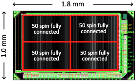
(a)

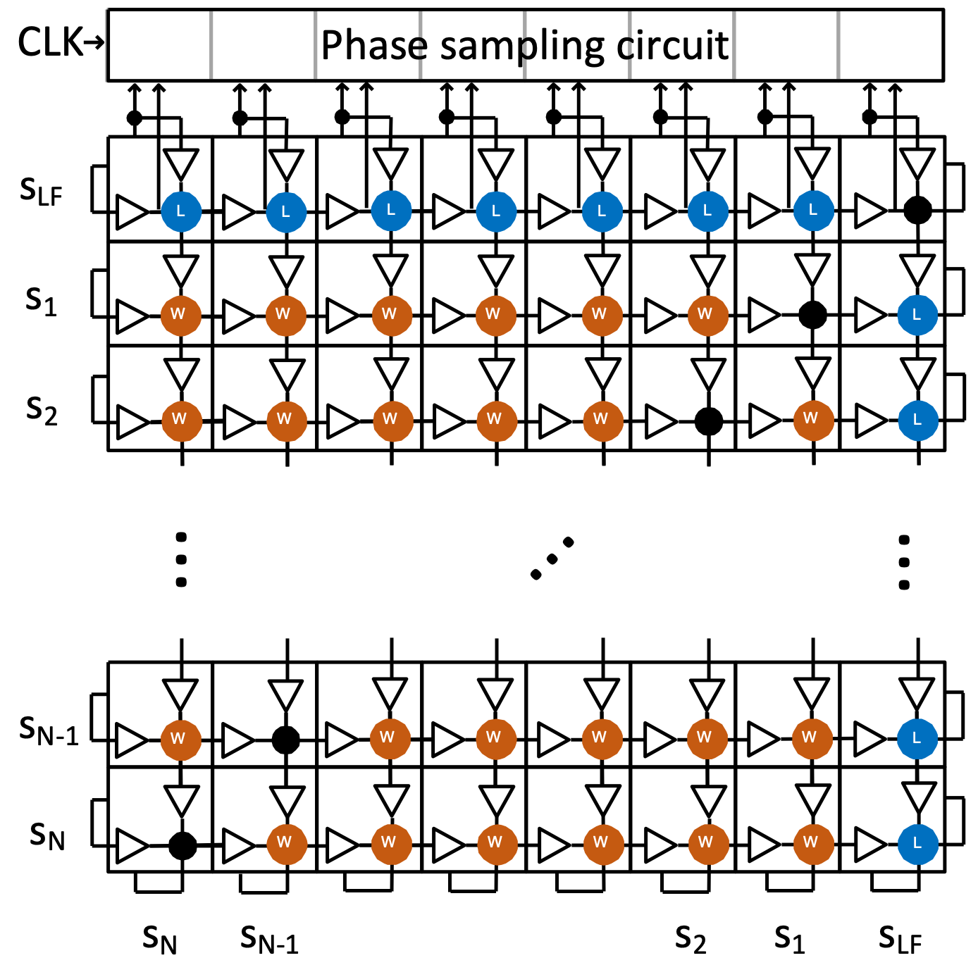
(b)

Figure 1: [6] (a) Chip layout and packaged chip soldered on a carrier board, attached to a Raspberry Pi. (b) All-to-all connected array of CMOS ROs.

III Degrees of Freedom in A2A Hardware Mapping

To solve a COP in Ising form on the A2A hardware of Section II-B, the process of mapping the Ising matrix and local field to the hardware must work within the hardware limitations. Since the coupling values $J_{ij}$ must be integers in the range $[-14,+14]$, smaller coupling weights of the problem may have to be upscaled while larger weights must be downscaled to lie in $[-14,14]$. This scaling step may result in non-integer values; these are rounded to an integer.

Conflicting considerations must be balanced during scaling: (1) The device accuracy is proportional to the coupling strength and therefore large scaling values are preferable. (2) If most of the weights are low in magnitude and only a few are high, it is possible that the lower weights will be zeroed out during downscaling. To avoid this, some coupling weights may be scaled beyond the dynamic range of the device and then clamped to the nearest extreme limit of the weight range. Excessive scaling/clamping may alter the coupling matrix so greatly that its solution departs from that of the original problem. Thus, scaling introduces trade-offs: we address them by dynamically reconfiguring the weight resolution of each spin.

A similar trade-off exists for the local field oscillators. The device allows an arbitrary number of spins to be configured as local field ROs (which implement $h_{i}$), while the remaining spins are configured to maintain pairwise coupling ($J_{ij}$ values). Increasing the number of Local Field Ring Oscillators (LFROs) can increase the dynamic range of the $h$ coefficients: for example, a single LFRO can allow a coupling weight in the range $[-14,+14]$; if we perform spin merging, where two LFROs are used (and coupled tightly) to represent a single spin, a weight range of $[-56,56]$ (as explained in the next paragraph) is allowable. In particular, if the effective dynamic range of the $h_{i}$s is larger than that of the $J_{ij}$s, then increasing the LFRO count can allow higher ranges for coupling values with less truncation, which is seen to result in improved accuracy. However, this also translates into fewer spin variables being available for problem mapping.

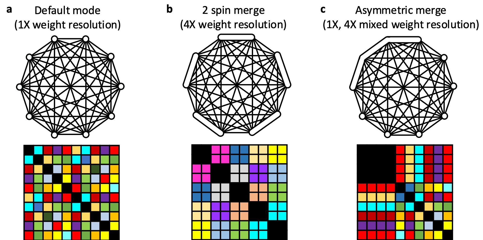
Figure 2: Illustrating spin-merging in the all-to-all array [6].

We illustrate spin merging in Fig. 2 [6] where a 10-spin hardware example is configured to a 10-spin default mode, a 5-spin 4× resolution mode, and a 6-spin asymmetric resolution mode, respectively. The graph (upper row) and the corresponding hardware mapping (lower row) are shown for each configuration. In the latter, the black weight cells connect the vertical and horizontal oscillators, and the coupling cells are color-coded according to coupling strength. When two spins are merged (middle figure), coupling sites (each with weights up to $\pm 7$) lie on two $2\times 2$ off-diagonal arrays. This allows coupling of $[-28,28]$ at each site and $J_{ij}\in[-56,+56]$. Thus, weight resolution can be traded off with the number of available spins.

IV Formulating 3SAT for an Ising solver

The Boolean satisfiability problem seeks to find an assignment of input variables for which a Boolean function evaluates to logic 1. The 3SAT problem was the “original” NP-complete problem, and 3SAT reduces to any other NP-complete problem through a polynomial-time transformation [9]. Therefore 3SAT is representative in the sense that its solutions can be used to obtain solutions to all NP-complete problems. Such problems span from practical challanges such as Traveling Salesman Problem [10] to numerous applications in electronic design automation [11].

A 3SAT instance in Conjuctive Normal Form (CNF) is a conjunction of clauses, i.e., $f(x_{1},\cdots,x_{n})=C_{1}\land C_{2}\land\cdots\land C_{m}$, where $X=\{x_{1},\cdots,x_{n}\}$ is a set of $N$ Boolean variables. Each clause $C_{i}=l_{1}\lor l_{2}\lor l_{3}$ is a disjunction of at most three literals $l_{1},l_{2},l_{3}\subset X\cup\neg X$. A SAT formula $f$ is satisfiable if there exists a set of Boolean assignments from $\{0,1\}$ on each variable in $X$ that can be substituted such that $f(x_{1},\cdots,x_{n})=1$; any combination of such variables, if it exists, is called a satisfying assignment.

Max-3SAT is a variant of the 3SAT problem that maximizes the number of clauses satisfied. If the solution of Max-3SAT says that all $N$ clauses are satisfiable, then the corresponding 3SAT problem is satisfiable [12]. The Max-3SAT problem can be formulated in QUBO/Ising Hamiltonians using multiple formulations, which we will describe next. We show these formulations in QUBO form; the spin formulation can be found as shown in Section II-A. The superscript against the name of each formulation provides the number of spins in the formulation as a function of $n$ and $m$.

IV-A The MIS^$3m$ Formulation

The maximal independent set (MIS) formulation [13] establishes a graph by assigning a QUBO variable (vertex) for each literal. For each clause, the three literals (vertices) are connected to each other, forming a “triangle” of edges. The literals of different clauses interact via conflict edges, which are formed if any two literals are negated versions of the same original Boolean variable. The triangle encourages the QUBO formulation to move to a new clause once a specific clause is satisfied, thus encouraging Max-3SAT, and penalizes conflicting assignments for the same variable. For a problem with $m$ clauses, this formulation requires $3m$ variables.

This formulation was translated into QUBO form in [14], using up to $3m$ QUBO variables, one for each vertex in the MIS formulation. Given an instance $C_{1}\lor C_{2}\lor\dots C_{m}=(l_{1}\lor l_{2}\lor l_{3})\land(l_{4}\lor l_{5}\lor l_{6})\land\dots\land(l_{3m-2}\lor l_{3m-1}\lor l_{3m})$, the QUBO Hamiltonian is:

$$\textstyle-\sum_{i=1}^{3m}l_{i}+2\left(\sum_{i=0}^{m-1}\sum_{j<k\in[1,3]}l_{3i+j}l_{3i+k}+\sum_{i,j|l_{i}=\neg l_{j}}l_{i}l_{j}\right)$$ (3)

where $\mathbf{l}$ is the vector of all literals in the expression. The minimized Hamiltonian represents the solution of the Max-3SAT problem.

The literals, $l_{i}$, have a many-to-one mapping to the original Boolean variables. If the literal values provide conflicting assignments to the Boolean variables, a majority vote is used to assign the value.

IV-B An ILP^$n{+}2m$ Formulation

Using the notation introduced above, we propose a new formulation representing the $i^{\rm th}$ clause by the Boolean inequality:

$$l_{3i+1}+l_{3i+2}+l_{3i+3}\geq 1$$

If the literal $l$ corresponds to variable $x$ in true form, then $l=x$; else $l=1-x$ if the literal is negated. The Max-3SAT problem can be represented as an integer linear program (ILP) that finds a feasible solution under these inequality constraints. Using a slack variable $s$, each inequality constraint is transformed to an equality constraint $l_{3i+1}+l_{3i+2}+l_{3i+3}-s-1=0$, where $s\in\{0,1,2\}$, depending on whether one, two, or all three literals are 1. Encoding $s=2s_{i,1}+s_{i,0}$, where $s_{i,1}$ and $s_{i,0}$ are binary variables, the equality constraint now contains all binary variables. To ensure this equality for each clause, the Hamiltonian minimizes the following sum of quadratics:

$$\textstyle\sum_{i=0}^{m-1}\left(l_{3i+1}+l_{3i+2}+l_{3i+3}-2s_{i,1}-s_{i,0}-1\right)^{2}$$

For example, clause $(x_{a}\lor x_{b}^{\prime}\lor x_{c})$ is encoded as $x_{a}+(1-x_{b})+x_{c}-2s_{1}-s_{0}-1=0$, and contribution to the Hamiltonian is the square of the left hand side. An instance with $n$ variables and $m$ clauses has $n+2m$ QUBO variables, including two ancillary slack variables for each of $m$ clauses. Typically, $n<m$, this has fewer Ising variables than MIS, but the range of weights is higher and the connectivity is denser. Unlike the MIS^3m formulation, where multiple variables represent the same literal and could potentially have contradictory assignments, there is a 1–1 correspondence between the first $n$ QUBO/Ising variables and the Boolean Max-3SAT variables.

IV-C The Chancellor^$n{+}m$ Formulation

The formulation in [15] maps an $n$-variable $m$-clause instance using $n+m$ QUBO/Ising variables. The formulation has a 1–1 correspondence between the $n$ SAT variables and the first $n$ QUBO/Ising variables, and adds one ancillary variable for each of the $m$ clauses. Denoting the SAT variables as $x_{1},\cdots,x_{n}$ and the ancillary variables as $x_{n+1},\cdots,x_{n+m}$, the overall Hamiltonian is:

$$\textstyle\sum_{i=0}^{m-1}\left(-(l_{n+i}+1)(l_{3i}+l_{3i+1}+l_{3i+2})+2l_{n+i}+\textstyle\sum_{j<k\in[0,2]}l_{3i+j}l_{3i+k}\right)$$ (4)

As in ILP^n+2m, for a literal $l$ in true form, $l=x$; else $l=1-x$.

IV-D The Nüßlein^$2n{+}m$ Formulation

The Nüßlein^$2n{+}m$ formulation [16] maximizes the number of satisfied clauses by making the Hamiltonian equal to the negative of the number of the satisfied clauses. For this purpose, a dual of each of the $n$ original variables is designated to obtain the variable pairs $x_{i},x_{i+1}$ that correspond to the $i^{\rm th}$ 3SAT variable. These are one-hot-encoded to 10 if the 3SAT variable is true, and 01 if it is false. Additionally, one ancillary variable is designated for each of $m$ clauses, leading to $2n+m$ variables. The QUBO weights are assigned according to the following Hamiltonian:

$$\textstyle{-}\sum_{i=1}^{2n}R(x_{i})x_{i}^{2}+2\sum_{i=2n+1}^{2n+m}x_{i}^{2}+\sum_{i=1|(i\mod 2)\not=0}^{2n-1}(m+1)x_{i}x_{i+1}$$

$$+\textstyle\sum_{i=1}^{2n}\sum_{j=1}^{2n}R(x_{i},x_{j})x_{i}x_{j}-\sum_{i=1}^{2n}\sum_{j=2n|x_{i}\in c_{j-2n}}^{2n+m}x_{i}x_{j}$$

where $R(x_{i})$ is the number of clauses that contain $x_{i}$, and $R(x_{i},x_{j})$ is similarly defined as the number of clauses such that contain both $x_{i}$ and $x_{j}$. This Hamiltonian aims to make the energy contribution of each satisfied clause $-1$ (and each unsatisfied clause $0$). The formulation then ensures that each variable is rewarded if it satisfies a clause (first term), and the local field coefficient of the ancillary variable of each clause is assigned to 2 (second term). Assignments of both a Boolean variable and its complement to 1 are penalized to ensure consistency (third term); the case where both are 0 effectively means that the variable is a don’t care.

IV-E The Nüßlein^$n{+}m$ Formulation

Although Chancellor^$n{+}m$ produces a relatively low number of QUBO variables than MIS^$3m$ and Nüßlein^$2n{+}m$, it uses relatively more coupling weights. The Nüßlein^$n{+}m$ formulation [16] has a lower number of nonzero couplings between QUBO/Ising variables.

Nüßlein^$n{+}m$ is based on four different clause literal negation patterns (provided in [16]) for Max-3SAT (where each pattern corresponds to the number of negated literals in the clauses). The formulation then consists of constructing (or updating) the Hamiltonian, clause by clause. Each pattern ensures that post(pre)-update Hamiltonian $H^{+}$($H^{*}$) satisfies $H^{+}=H^{*}$ if the immediate clause is satisfied, and $H^{+}=H^{*}+1$ otherwise. Based on this rule and the negation pattern of each clause, the Hamiltonian is updated iteratively for each clause. An advantage is the possibility of reusing clause variables; in the worst case, the number of clause variables is $m$, as in Chancellor^$n{+}m$.

V Workflow of our Hybrid Approach

V-A Overview of our Hybrid Solver Approach

Any hardware solver is limited in the number of spins that it can represent. Larger problems must be decomposed into smaller subproblems that can fit on the hardware and solved iteratively until the ground state is found. The qbsolv [17] engine performs a similar decomposition, purely in software, optimizing a large QUBO problem by solving a series of sub-QUBO problems using local Tabu search.

Our workflow for 3SAT solution and evaluation is illustrated in Fig. 3. We show a hybrid hardware-based flow and a purely software-based flow. The software flow is based on qbsolv, but augmented with new methods that we propose for problem decomposition.

The software approach effectively emulates the A2A hardware results, but is free of nonidealities and noise associated with a hardware implementation of an Ising solver, and should represent the best achievable results for the hardware-based flow. Therefore, we use the software flow to evaluate the effectiveness of various Ising formulations (Section IV) and decomposer schemes (Section V-B). We evaluate this pruned list of candidates on the Ising hardware. The advantage of this two-step approach is that the hardware, which is an experimental university project, currently focuses on optimizing the core A2A engine but has slow I/O. This makes hardware evaluation of all algorithms and decomposers time-intensive. This I/O bottleneck is a temporary artifact and is easily resolved: future versions of the chip, currently in the tapeout stage, are addressing this issue [18].

In the figure, the blue boxes represent segments common to both solutions, and are performed on a classical computer. We first transform the 3SAT problem, consisting of variables and clauses, into a global Hamiltonian (Ising) formulation, as described in Section II-A. The size of the Hamiltonian depends on the 3SAT problem and the specific formulation used to map 3SAT to QUBO, as described in Section IV. Typically, the Ising global Hamiltonian involves a large number of spins that cannot be directly mapped onto an on-chip RO array. To address this, we use a decomposer to generate an Ising sub-Hamiltonian that can fit the dimensions of the RO array: on the A2A hardware, this allows at most 49 spins, including the reference.

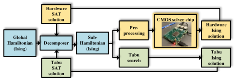
Figure 3: Workflow of our hybrid solver.

For hardware-based evaluation (yellow boxes in Fig. 3), this sub-Hamiltonian is taken through a preprocessing step (Section V-C), and the Ising weights are then programmed on to the RO-based Ising chip. The spin solution on the chip is sampled to determine the phase for each RO using majority voting. This represents the Ising solution for the sub-Hamiltonian, from which the SAT solution is inferred. To assess the accuracy of our RO solver, we also utilize a software-based Tabu search [19], as in qbsolv [17], to solve the same sub-Hamiltonian as a control group (green boxes in Fig. 3) to find a Tabu spin solution from which we infer the SAT solution.

For both hardware-based and software-based evaluation, after the solution of the current sub-Hamiltonian, the decomposer sends the next sub-Hamiltonian for processing. This terminates after checking whether all clauses are satisfied, i.e., “all-SAT” is achieved, or if a predefined iteration limit is reached. When a single SAT variable is determined by multiple spins (e.g., MIS^3m), it is crucial to identify and report contradictions when converting the Ising solution back to the SAT solution. Section VI will delve deeper into these issues.

V-B Decomposers

We study five decomposers: the last three are developed by us.

Energy impact decomposer. This decomposer, the qbsolv default, arranges all spins in ascending order based on their flip energy (i.e., the energy difference when spin $s_{i}$ is flipped to $-s_{i}$), and then selects spins with the highest flip energy to construct the sub-Hamiltonian. However, such a greedy algorithm has a higher probability of being trapped in a local minimum where all spins have positive flip energy.

Random decomposer. This decomposer randomly selects spins from the global Hamiltonian to form the sub-Hamiltonian. The randomness in the selection process helps the algorithm escape from local minima.

Pseudorandom decomposer. Our heuristic scheme continually reshuffles and shifts the variable order, selecting the first $S$ variables at each iteration for the sub-Hamiltonian solver, where $S$ represents the number of spins supported by the hardware. The pseudorandom decomposer offers a lower probability of selecting the same spins in subsequent iterations than the Random decomposer, resulting in greater diversity among the generated sub-Hamiltonians.

BFS decomposer. This scheme creates a cluster around a randomly-selected source vertex in the Ising graph. A breadth-first search (BFS) in the graph starts from the source, adding neighbors of vertices in randomized order until the sub-problem capacity is reached.

SAT decomposer. This clustering-based decomposer randomly selects one clause at each step and adds all spins related to the selected clause and its involved variables to the sub-Hamiltonian.

V-C Preprocessing for RO Array

The decomposed sub-Hamiltonians generated above must be further processed to work within the restrictions imposed by the Ising chip:

1. Coupling values must be integers in $[-14,+14]$; couplings for 3SAT formulations are integers, but may go out of this range.

2. Empirically, it is seen that the device accuracy is proportional to the coupling strength, and large coupling values are preferable.

3. Empirically, device accuracy decreases for lower graph density.

Therefore, we preprocess the Ising Hamiltonian, translating the original sub-Hamiltonian from the decomposer to a hardware-compatible sub-Hamiltonian coupling matrix, using the following methods (these are applied to the hardware flow, not the software flow):

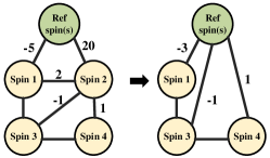
Figure 4: An example where spin 2 can be removed (set to the reference spin).

Mapping: As mentioned in Section III, increasing the number of LFROs and using spin merging to implement the local field can increase the dynamic range of the $h$ coefficients, to improve the solving accuracy. In Section VI, we sweep the number of LFROs to locate the optimal number of LFROs to obtain an empirical value for the number of LFROs to be merged.

Removing spin variables from the sub-Hamiltonian: When the local field on a spin variable is very large, it will force the variable to a fixed value. The contribution of a spin $s_{i}$ on the Ising Hamiltonian is $H(s_{i})=h_{i}s_{i}+\textstyle\sum_{j=1,j\not=i}^{n}J_{ij}s_{i}s_{j}$. Then the flip energy
$H_{flip}(s_{i})=H(s_{i}$$=$$+1)-H(s_{i}$$=$$-1)=2\left(h_{i}+\textstyle\sum_{j=1,j\neq i}^{n}J_{ij}s_{j}\right)$
A lower bound smallest value of the second term is $\textstyle-\sum_{j=1,\\ j\neq i}^{n}|J_{ij}|$. Thus, if $h_{i}>0$, then regardless of the choice of the other spins,

$$H_{flip}(s_{i})\geq 2\left(h_{i}-\textstyle\sum_{j=1,j\neq i}^{n}|J_{ij}|\right)$$ (5)

If $h_{i}>\sum_{j=1,j\neq i}^{n}|J_{ij}|$, then $H(s_{i}=+1)>H(s_{i}=-1)$, i.e., a minimum Hamiltonian will force $s_{i}=-1$. Similarly, if $H_{flip}(s_{i})\leq 2(h_{i}+\sum_{j=1,j\not=i}^{n}|J_{ij}|)<0$, i.e., $h_{i}<-\sum_{j=1,j\not=i}^{n}|J_{ij}|$, then it can be shown that $s_{i}=+1$ at a minimum Hamiltonian value.

Together, these cases show that if $h_{i}$ is very negative [very positive], $s_{i}$ must be $+1$ [$-1$] at the minimum, and the corresponding spin variable can be removed from the Hamiltonian. Since the weights in the hardware are limited to $[-14,+14]$, this serendipitously allows us to remove large/small weights, at no loss of accuracy.

In practice, we use the criterion $|h_{i}|>N\times\max_{j}|J_{ij}|$, for a tuned value of $N$, and find it to be effective in identifying spins that could be removed, empirically without loss of optimality. In Fig. 4, the coupling between spin 2 and reference spin (Ref) $h_{2}=20$ is much larger than $\max_{j}J_{2j}=2$. Therefore, spin 2 is removed from the Hamiltonian. All couplings, $J_{2j}$, are transferred into couplings with the reference spin ($h_{j}$), and spin 2 is set to $+1$.

Scaling: Since large coupling values are preferable for device accuracy, and minimizing $F(\mathbf{s})$ in (2) is identical to minimizing $kF(\mathbf{s})$ for any scalar $k$, we can scale the $h_{i}$ and $J_{ij}$ values up as long as the maximum value lies in the range $[-14,+14]$. If a few spins go slightly above $\pm 14$, these may be truncated, as described next.

Truncation: Coupling values beyond $\pm 14$ can be truncated by clamping them to $=14$ or $-14$, whichever is closer.

VI Experimental Setup and Metrics

We present three experiments in this section: (1) a software simulation, focusing on Hamiltonian formulations and choices for the decomposer; (2) a hardware sub-Hamiltonian test, focusing on preprocessing; (3) using the optimal configuration from the first two experiments to solve 3SAT benchmarks using our complete workflow.

We use 10 benchmarks from the SATLIB uf20-91 suite [20]. All benchmarks are satisfiable and each includes 20 variables/91 clauses. With a clauses-to-variables ratio, $(m/n)$ of 4.55, these problems lie close to the phase transition region [21], where about half of the SAT instances are satisfiable and the rest are unsatisfiable: the hardest SAT problems lie in this region. We use the following metrics:

Iterations: In each iteration in the inner loop of our workflow, the decomposer generates a sub-Hamiltonian, sent to the Ising solver. The 3SAT problem is solved over multiple sub-Hamiltonian solutions.

Repeats: 3SAT/Hamiltonian solving is repeated many times in the outer loop of our workflow, thus reducing the impact of the random initial state of the chip, which may trap solutions in local minima.

All-SAT rate: This quality metric is the number of repeats that find an all-SAT solution, divided by the total number of repeats.

Energy rate: This is the ratio of the sub-Hamiltonian energy of the current solution and the ground state (from the software workflow), and indicates the accuracy of the sub-Hamiltonian solution.

Next, we first sweep through different formulation and decomposer combinations using software-based solvers in Section VI-A. We adapt the D-Wave Hybrid solver and replace its internal decomposition algorithm with the candidate decomposers from Section V-B, and determine the best-performing formulation+decomposer in an “ideal” environment. In Section VI-B, we perform Ising accelerator hardware parameter sweeps to maximize the solution accuracy for sub-Hamiltonian Ising problem instances. Finally, we combine software and hardware optimizations in Section VI-C to solve 3SAT instances.

VI-A Decomposer and Formulation Results

In Fig. 5, we explore the different Ising formulations of the 3SAT problem alongside different decomposition strategies using software-only subsolvers (i.e., Tabu search). The figure shows the average All-SAT rate out of 100 repeats for the first 10 instances in the uf20-91 benchmarks, using multiple formulations and decomposers, over 500 iterations. The results show the All-SAT rate at the end of 50, 100, and 500 iterations, as denoted with darker-to-lighter tones from bottom to top in each bar. We conclude that the best performance comes from the Chancellor^$n{+}m$ formulation and the BFS decomposer.

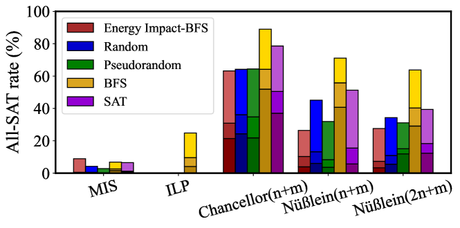
Figure 5: Evaluation of various formulations and decomposers (the pseudorandom, BFS, and SAT are developed in this work).

VI-B Hardware Optimization Results

In order to optimize the parameters that improve the subsolution accuracy on the hardware, we show the effects of scaling and mapping (i.e., number of LFROs) in Fig. 6. Individual software and chip energies for the subproblems that are constructed through decomposition for uf20-91/01 benchmark are provided in Fig. 6(a) for a scaling factor of 2 (i.e., all couplings are multiplied by 2) and in Fig. 6(b)–(d) for scaling by 12 with 2, 4, and 10 LFROs, respectively. Scaling is used together with truncation, clamping values beyond $\pm 14$. Note that Fig. 6(a) has a significant discrepancy between the ideal and hardware Hamiltonian energies, while in Fig. 6(c) with higher scaling and the same number of LFROs, the hardware follows the software much more closely due to the stronger coupling of spins, thus reinforcing the empirical observation that stronger coupling improves chip accuracy. At the higher scaling factor of 12, it is seen that 2 LFROs in Fig. 6(b) provide better accuracy than the Scale 2 case, but that 4 and 10 LFROs in Fig. 6(c) and (d), respectively, provide progressive improvements. This is because the larger number of LFROs have sufficient dynamic range to accommodate $h$ coefficients with fewer truncations. Therefore, appropriate selection of scaling factors and the LFROs can make hardware subproblem solutions more closely follow the software-based ground state solutions.

(a) Scale=2, LFROs=4

(b) Scale=12, LFROs=2

(c) Scale=12, LFROs=4

(d) Scale=12, LFROs=10

Figure 6: Software and chip Hamiltonian energy for uf20-91/01 instance, (a) for Scale 2 with 4 LFROs; for Scale 12 with (b) 2, (c) 4, and (d) 10 LFROs.

We sweep the scaling factor and the number of LFROs, and based on the statistics of subproblem accuracy, we choose an optimal point of peak accuracy at a scaling factor of 12, and a choice of 4 LFROs.

VI-C 3SAT Results with Ising Accelerator

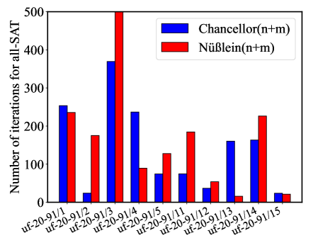
(a)

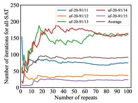
(b)

Figure 7: Number of iterations to find All-SAT for hardware test on the Ising chip for (a) Average number of iterations for uf20-91/(01-05, 11-15) for Chancellor^$n{+}m$ and Nüßlein^$n{+}m$ (b) Average number of iterations with repeats for uf20-91/(11–15) in the formulation of Chancellor^$n{+}m$.

Based on Fig. 5, we select the best two formulations (Chancellor^$n{+}m$ and Nüßlein^$n{+}m$) and use their best decomposer (BFS) to setup our Hybrid 3SAT solver. We use instances 01–05 of uf20-91, which were used in our previous optimization, and an orthogonal set, instances 11–15 of uf20-91, which were never used in any previous experiments to optimize our hybrid solver. Over 100 repeats for each benchmark, with a time-out at 500 iterations, we plot the average number of iterations to reach all-SAT in Fig. 7(a) for the Chancellor^${n{+}m}$ and Nüßlein^$n{+}m$ formulations, over all 10 instances. In general, the Chancellor formulation is better as it achieves all-SAT in fewer iterations than Nüßlein, with a few exceptions, e.g., uf20-91/13. However, in one case (uf20-91/03), the Nüßlein formulation is unable to achieve all-SAT over the 100 repeats, as shown by the average number of iterations being at the time-out limit of 500. Fig. 7(b) shows the evolution of the average number of iterations over 100 repeats for instances 11–15. After some repeats, the average settles to the steady-state value in Fig. 7(a).

Table I: Runtime estimation for our Hybrid solver.

	Runtime per	Multiplier for	Number of	Runtime
	unit operation	previous column	repeats	(ms)
Input	$1.25\times 10^{-3}\mu$s/bit	9604 bits	1	12.0$\mu$s
RO relaxation	(1/26MHz) s/cycle	40 cycles	100	153.8$\mu$s
Output	$1.25\times 10^{-3}\mu$s/bit	49 bits	100	6.1$\mu$s
Overall runtime				171.9$\mu$s

Runtime analysis. A runtime analysis of our Hybrid solver is illustrated in Table I, assuming 100 repeats and 100 iterations per repeat and finds the one with minimal Hamiltonian, which is consistent with Fig. 5. As an academic demonstrator, with a focus on optimizing the all-to-all array, the Ising chip has several limitations:
(1) It has low IO bandwidth – but this is not a fundamental bottleneck. The authors of [6] indicate that they can achieve 800Mbps in a future version of the chip [18] with 8-bit parallel IO at 100Mbps each.
(2) Majority voting (Section II-B) is performed externally on a CPU, but can easily be incorporated in a small on-chip circuit. With this on-chip voting engine, the output data can be reduced from 8 bits/spin to 1 bit/spin, so that 49 spins only generate 49 bits of output.
(3) The Hamiltonian computation to check for convergence is currently performed off-chip, using the Ising energy computation function in the dimod [22] package on an Intel Xeon 4114 CPU. This currently takes 3.6ms, and in a currently taped-out advanced version of the Ising chip, this computation is performed in hardware [18]. The on-chip Hamiltonian computation is overlapped with the next Ising solution, and therefore incurs no additional latency.
All of these are relatively simple extensions, and the only reason that they are not on the chip already is because it is an academic project, limited by the number of students who can work on tape-outs; nevertheless, these enhancements are already in the pipeline in chips that are taped out or will be taped out shortly [18]. To project the true power of this hardware computational model, we use the settling time of the current version of the Ising chip, and project the total runtime numbers under the assumption that the above three improvements are made. Under these assumptions, the overall runtime is 171.9$\mu$s. Given that the software Tabu search usually takes 10-100ms, and the default timeout value is 100ms in D-Wave Hybrid [23], our hybrid solver can solve 3SAT problems orders of magnitude faster than a software-based solver. A preliminary experiment on a small 3SAT instance, which can fit on the Ising chip without decomposition, shows a 10$\times$ runtime improvement over a classical SAT solver, MiniSAT [24].

References

- [1] A. Lucas, “Ising formulations of many NP problems,” Front. Phys., vol. 2, pp. 5:1–5:15, 2014.
- [2] K. Boothby et al., “Next-generation topology of D-Wave quantum processors,” arXiv:2003.00133, 2020.
- [3] M. Yamaoka et al., “A 20K-spin Ising chip to solve combinatorial optimization problems with CMOS annealing,” IEEE J. Solid-St. Circ., vol. 51, no. 1, pp. 303–309, Jan. 2016.
- [4] I. Ahmed et al., “A probabilistic compute fabric based on coupled ring oscillators for solving combinatorial optimization problems,” IEEE J. Solid-St. Circ., vol. 56, no. 9, pp. 2870–2880, Sep. 2021.
- [5] W. Moy et al., “A 1,968-node coupled ring oscillator circuit for combinatorial optimization problem solving,” Nature Electron., vol. 5, no. 5, pp. 310–317, 2022.
- [6] H. Lo et al., “A 48-node all-to-all connected coupled ring oscillator Ising solver chip,” 2023, doi.org/10.21203/rs.3.rs-2395566/v1.
- [7] “Programming the D-Wave QPU: Setting the chain strength,” 2020, dwavesys.com/media/vsufwv1d/14-1041a-a_setting_the_chain_strength.pdf.
- [8] Z. I. Tabi et al., “Evaluation of quantum annealer performance via the massive MIMO problem,” IEEE Access, vol. 9, pp. 131 658–131 671, 2021.
- [9] R. M. Karp, “Reducibility among combinatorial problems,” in Complexity of Computer Computations. New York, NY: Plenum Press, 1972.
- [10] S. N. Kabadi and A. P. Punnen, “The bottleneck TSP,” in The Traveling Salesman Problem and its Variations, G. Gutin and A. P. Punnen, Eds. Boston, MA: Springer, 2007, pp. 697–735.
- [11] L.-T. Wang et al., Electronic Design Automation: Synthesis, Verification, and Test. San Francisco, CA, USA: Morgan Kaufmann, 2009.
- [12] W. Zhang, “Phase transitions and backbones of 3-SAT and maximum 3-SAT,” in Principles and Practice of Constraint Programming, T. Walsh, Ed. Berlin, Germany: Springer, 2001, pp. 153–167.
- [13] S. Dasgupta et al., Algorithms. New York, NY: McGraw Hill, 2008.
- [14] V. Choi, “Adiabatic quantum algorithms for the NP-complete maximum-weight independent set, exact cover and 3SAT problems,” arXiv:004.2226, 2010.
- [15] N. Chancellor et al., “A direct mapping of max k-SAT and high order parity checks to a Chimera graph,” Sci. Rep., vol. 6, no. 1, pp. 37 107:1–37 107:9, 2016.
- [16] J. Nüßlein et al., “Solving (max) 3-SAT via quadratic unconstrained binary optimization,” arXiv:2302.03536, 2023.
- [17] “qbsolv,” 2018, github.com/dwavesystems/qbsolv.
- [18] C. H. Kim, “Private communication,” 2023.
- [19] F. Glover and M. Laguna, Tabu Search. Boston, MA: Springer US, 1998, pp. 2093–2229.
- [20] “uf20-91,” 2023, www.cs.ubc.ca/~hoos/SATLIB/benchm.html.
- [21] D. Mitchell et al., “Hard and easy distributions of SAT problems,” in Proc. AAAI Conf. Artif. Int., 1992, pp. 459–465.
- [22] “dimod,” 2018, github.com/dwavesystems/dimod.
- [23] “D-Wave Hybrid,” 2023, github.com/dwavesystems/dwave-hybrid.
- [24] “Minisat,” minisat.se.