COSE: A Consistency-Sensitivity Metric for Saliency on Image Classification

Abstract

We present a set of metrics that utilize vision priors to effectively assess the performance of saliency methods on image classification tasks. To understand behavior in deep learning models, many methods provide visual saliency maps emphasizing image regions that most contribute to a model prediction. However, there is limited work on analyzing the reliability of saliency methods in explaining model decisions. We propose the metric COnsistency-SEnsitivity (COSE) that quantifies the equivariant and invariant properties of visual model explanations using simple data augmentations. Through our metrics, we show that although saliency methods are thought to be architecture-independent, most methods could better explain transformer-based models over convolutional-based models. In addition, GradCAM was found to outperform other methods in terms of COSE but was shown to have limitations such as lack of variability for fine-grained datasets. The duality between consistency and sensitivity allow the analysis of saliency methods from different angles. Ultimately, we find that it is important to balance these two metrics for a saliency map to faithfully show model behavior.

1 Introduction

Given a function $f$ operating on images $x\in\mathbb{R}^{m\times n\times c}$, a saliency map $M\in\mathbb{R}^{m\times n}$ indicates the relative importance of each pixel in the image $x$ in making the prediction $f(x)$. Saliency maps have been widely used to understand (possibly black-box) function behavior, especially with deep networks. They are important for humans to establish trust in predictions through transparency, and have been applied in high-stakes decisions such as medical diagnoses [24] and bias identification [22]. Given saliency techniques are inextricably linked to human understanding, saliency maps should fulfill certain properties based on our understanding of the visual system in the world around us.

We propose consistency and sensitivity metrics that measure two complementary properties of saliency maps. Consistency refers to the property that saliency maps should remain unchanged when an input is transformed in a way that the model predictions don’t change. For example, when an input is reflected or translated by a small amount, the corresponding saliency maps should also undergo the same geometric transformation, as we do not expect the class predictions to change. Similarly, when the input undergoes a photometric transformation (e.g., change in pixel intensities or blurring), we expect saliency maps to remain identical. In short, consistency captures the degree to which saliency maps are equivariant and invariant to transformations that don’t affect model predictions. Sensitivity refers to the property that saliency maps should change when the model produces a different output. This difference in model output could be a result of changes in the model parameters (e.g., during the process of training the model) or sufficiently large changes in input. Thus, the model’s explanations must change for it to produce a different output. Prior knowledge was used to identify transformations that should result in equivariance and invariance for various computer vision tasks.

While prior work has focused on evaluating consistency of saliency maps [31, 26, 35, 12], we show that sensitivity is also a key consideration and often in conflict with consistency. We propose a combined metric called COSE defined as the harmonic mean of the consistency and sensitivity. Our work also considers natural changes to the input, and model perturbations that occur in realistic training settings.

We develop a benchmark where we evaluate several saliency methods [22, 4, 24, 29, 13, 23, 21], deep network architectures [9, 17, 7, 16], pre-training procedures [3, 5, 34, 25], and evaluate these metrics on five different datasets [14, 15, 28, 11, 20]. We find that saliency maps generally produce more coherent explanations on transformer-based models than convolutional-based models. GradCAM also demonstrates better performance across the different metrics and across the different evaluation settings when compared to other methods. Finally, we observe common limitations among saliency methods on balancing consistency and sensitivity, and we recommend future directions for the improvement of saliency methods. In summary, our contributions include the following:

• We propose the metrics consistency, sensitivity, and COSE to evaluate the robustness of saliency methods to input and model changes based on vision priors.

• We introduce an evaluation pipeline that incorporates natural image and model variations encountered by human end users which we open source for future research.

• We show the effectiveness of our proposed metrics to evaluate different model architectures (with supervised and unsupervised features) to analyze the behavior of saliency methods across different settings.

2 Related Work

2.1 Saliency Maps

Saliency explanations generally attribute importance to input features [1]. For images, explanations typically are represented as saliency heatmaps, in which “important” pixels are highlighted. Most explainability methods either involve gradient and activation summation [22, 4], input perturbations [21], or some combination of both [24, 29, 13, 23].

CAM methods One popular form of saliency maps is class activation mapping (CAM) [32], which sums activations within a layer of the network to produce heatmaps, weighted by a value related to the output classification. We consider two variants of CAM known as GradCAM and GradCAM++. GradCAM weights using the average gradient with respect to the desired output classification [22], and GradCAM++ builds on this idea but uses second-order gradients to produce explanations with improved object localization [4].

IG methods On the other hand, Integrated Gradients (IG) linearly interpolates between a baseline input (in our case, a black image) and the target input while summing the gradient of the output along the path [24]. In a variant called BlurIG, the path is not linear but generated by constantly blurring the original image using the Laplacian of Gaussian kernels [29]. Meanwhile, Guided IG follows an adaptive path along pixels with the smallest derivative with respect to the output [13].

Other methods We also looked at two methods unrelated to IG and CAM. SmoothGrad averages the gradient of the classification output with respect to noisy version of the input image [23]. This method can also be combined with other methods such as IG, but we used the method with vanilla gradients highlighted in the paper. Meanwhile, LIME approximates the model behavior in the neighborhood of a given input using a simple linear model to generate sparse explanations [21].

2.2 Saliency Metrics

Although defining which explanations are helpful or unhelpful can be a challenging task [1], several qualitative characteristics for good explanations have been proposed, including fidelity to model prediction and generalizability across explanations [24, 31, 8]. Various quantitative metrics have been developed to examine these properties, but we found these methods either required unnatural, out-of-distribution perturbations or have focused on examples that were not meaningful for explaining typical neural network use cases.

Model perturbation. Some methods randomize parts or all of the weights in a neural network and expect explanations to change [1, 2], but we question whether the effects of manual changing sections of a network on corresponding explanations can be reliably predicted. Instead, we do this in a less artificial way by saving checkpoints of the model as it is being trained, ensuring we are able to produce models in the same way as a typical user might in the process of training of fine-tuning models.

Input perturbation. Similarly, many metrics perturb inputs and observe how explanations change in order to measure the quality of an explanation [31, 26, 35, 12]. In all examples we investigated, these perturbed inputs are not in the training distribution, and we believe it is difficult to justify that explanations should change or stay the same. In contrast, we use augmentations which are in the training distribution to guarantee that the network should behave in the same way as in training and thus should explain predictions in the same way.

Generating ground truth explanations. Zhou et al. randomizes dataset labels to coincide solely with a single image augmentation, implying this augmentation is the ground-truth explanation for this dataset [35]. Similarly, the BAM dataset generates an artificial dataset by pasting images from one dataset to another and training models in such a way that the feature importance is known [30]. Fel et al. bootstraps networks with different test sets and anticipates the explanations to be the same between networks which trained on a given input and those which only encounter the input in the test set [8]. While these methods are informative, they fail to capture the full story of a typical usage of neural networks on a natural dataset.

Human studies. Zimmermann et al. tries to evaluate the usefulness of visual explanations by having users predict network activations with and without visual aids [36]. Using human studies is sensible given the explanations are meant to improve human understanding, but can be difficult to formulate and expensive to implement. Quantitative methods can help analyze other factors and narrow down methods to examine more closely [33].

Similarity between explanations. Methodology for determining similarity or distance scores between two explanations quantitatively is not evident a priori, and prior works are somewhat divided between various methods including Spearman rank correlation [26, 8], structural similarity index (SSIM) [2, 1], and Pearson correlation on the histogram of gradients for each explanation [1]. We chose in this work to use structural similarity index because of its applicability to images based on human perception. We explored using Pearson correlation instead of SSIM and found similar results presented in the supplementary material.

3 Method

3.1 Problem Formulation

We focus on evaluating the performance of saliency methods on supervised classification models trained on a set of data points $D=\{(x_{1},y_{1}),(x_{2},y_{2}),\ldots,(x_{n},y_{n})\}$ where $x\in X$ is an input image and $y\in Y$ is the class label of the image. A model learns a function $f:X\to Y$ that estimates $\hat{y}$ from the given $x$, where $\hat{y}$ is as close as possible to $y$. A saliency method $\Phi$ tries to estimate a map $M_{i}\in[0,1]^{m\times n}$ from a given input image $x_{i}\in\mathbb{R}^{m\times n\times c}$, its corresponding output $\hat{y_{i}}\in\mathbb{R}^{d}$, and the model $f$. More formally, saliency maps can be represented as:

$$\Phi(f,x_{i})=M_{i}$$ (1)

To evaluate saliency methods, we measure changes in $M_{i}$ by varying either $x_{i}$ or $f$. The next subsections discuss these modifications to the input and the model, and propose measurements on saliency maps that capture their performance and reliability.

3.1.1 Data Augmentations

The data augmentation module applies natural image transformations to represent image variation observed in the wild. To ensure these augmentations are simple, replicable, and reversible, we use a subset of transformations in TrivialWideAugment [19], which randomly applies a single augmentation with random magnitude. Each transformation is either a fixed magnitude (e.g. flipping the image) or uniformly sampled from a discrete, linearly spaced set of 61 magnitudes. We removed transformations we deemed to be not naturally occurring, such as shearing. We define photometric transformations as those which vary the perceived colors of the images (e.g. varying the contrast), whereas geometric transformations vary the orientation of the images (e.g. rotation, translation). We classify geometric transformations as the set $G$ and photometric transformations as the set $H$ and let $T=G\cup H$.

A model $f$ is invariant to the data transformation $t\in T$ if $f(x_{i})\equiv f(t(x_{i}))$. We define a saliency map $\Phi(f,x_{i})$ as being equivalent to $\Phi(f,t(x_{i}))$ if it is equivariant to geometric data transformations and invariant to photometric data transformations. In other words, for $h\in H$, we expect $\Phi(f,x_{i})=\Phi(f,h(x_{i}))$, while for $g\in G$, we reverse the operation on the saliency maps before evaluation, meaning we expect $\Phi(f,x_{i})=g^{-1}(\Phi(f,g(x_{i})))$.

On the other hand, data transformations that result to a different model output $f(x_{i})\not\equiv f(t(x_{i}))$ should also correspond to different saliency maps $\Phi(f,x_{i})\not\equiv\Phi(f,t(x_{i}))$. Figure 2 shows this on a sample image using GradCAM where consistent model behavior should result to equivalent saliency maps, and changing model behavior should result to different saliency maps.

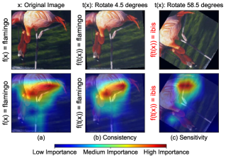
Figure 2: GradCAM consistency and sensitivity to data transformations on ResNet50/Caltech101: the top row shows the input images, and the bottom row shows the corresponding saliency maps. In the reference image (a), the model correctly classifies the original image as a flamingo. (b) displays GradCAM’s consistency as the model correctly classifies the transformed image ($f(x)\equiv f(t(x_{i}))$) with a similar saliency map as (a). (c) displays GradCAM’s sensitivity where the model incorrectly classified the transformed image as ibis $\left(f(x)\not\equiv f(t(x))\right)$ and the saliency map emphasizes differently from (a).

3.1.2 Model Augmentations

Prior to training, models have random weights and are unable to classify properly. As a model learns, the underlying weights change and adapt to the data presented. Given the main goal of saliency maps is to clarify the behavior of the underlying model, saliency maps should display the model changes as it undergoes training. When the model updates from $f^{\prime}\rightarrow f$, the corresponding saliency map should also evolve $\Phi(f^{\prime},x_{i})\rightarrow\Phi(f,x_{i})$.

To have realistic changes in model weights, we capture the changing model as it is trained from the first epoch until it reaches the final trained state. In the final state, the model should have learned where and how to look at the images and classify images correctly. We quantify this performance using the test set classification accuracy. In other words, we should see that as a model learns, the saliency maps should reflect the increasing accuracy of this changing model.

3.2 Proposed Metrics

Structural Similarity Index Measure (SSIM) [27] is used on the saliency maps to quantify the deviation of maps due to variations from data and model augmentations. Equation 2 defines the similarity of two maps $M_{x}$ and $M_{y}$ using $\operatorname{SSIM}$, which lies between 0 and 1. The variable $\mu_{M_{x}}$ is the pixel sample mean of $M_{x}$, $\sigma_{M_{x}}^{2}$ is the variance of $M_{x}$, and $C_{1}=0.01,C_{2}=0.03$ are variables to stabilize the division for small denominator values. Subsequent sections on the proposed metrics will use this similarity measure for comparing two output saliency maps.

$$\operatorname{SSIM}(M_{x},M_{y})=\frac{\left(2\mu_{M_{x}}\mu_{M_{y}}+C_{1}\right)\left(2\sigma_{M_{x},M_{y}}+C_{2}\right)}{\left(\mu_{M_{x}}^{2}+\mu_{M_{y}}^{2}+C_{1}\right)\left(\sigma_{M_{x}}^{2}+\sigma_{M_{y}}^{2}+C_{2}\right)}$$ (2)

3.2.1 Consistency

Based on the idea described in § 3.1.1, we propose the consistency metric. The metric measures the robustness of saliency maps to data augmentations. Given a model robust to a set of data augmentations, reliable saliency maps should show equivalent explanations for the input $x_{i}$ and its transformed counterpart $t(x_{i})$ (Equation 3).

$$f(x_{i})\equiv f(t(x_{i}))\implies\Phi(f,x_{i})\equiv\Phi(f,t(x_{i}))$$ (3)

Let $(X,H)^{*}$ be a set such that for $x\in X$ and $h\in H$, $(x,h)\in(X,H)^{*}$ if and only if $f(x)\equiv f(h(x))$ and similarly for $(X,G)^{*}$. We evaluate the robustness of a given method $\Phi$ based on the similarity of the two maps and propose the following consistency metric:

$$\operatorname{consistency}=\frac{1}{N}\sum_{(x,h)\in(X,H)^{*}}\operatorname{SSIM}(\Phi(f,x_{i}),\Phi(f,h(x_{i})))\\ +\frac{1}{N}\sum_{(x,g)\in(X,G)^{*}}\operatorname{SSIM}(\Phi(f,x_{i}),g^{-1}(\Phi(f,g(x_{i})))),$$ (4)

where $N=|(X,H)^{*}\cup(X,G)^{*}|$.

3.2.2 Sensitivity

Complementing the idea of consistency, if a model prediction changes due to either a change in input (§ 3.1.1) or a change in the model itself (§ 3.1.2), an optimal saliency method should also reflect these changes. We call this characteristic sensitivity. A saliency method should be sensitive to the underlying changes in the model itself (Equation 5) or to the response of a model to an input augmentation $t\in T$ (Equation 6).

$$f(x_{i})\not\equiv f^{\prime}(x_{i})\implies\Phi(f,x_{i})\not\equiv\Phi(f^{\prime},x_{i})$$ (5)

$$f(x_{i})\not\equiv f(t(x_{i}))\implies\Phi(f,x_{i})\not\equiv\Phi(f,t(x_{i}))$$ (6)

We reformulate minimizing $\operatorname{SSIM}$ to instead maximize $d(M_{1},M_{2})=1-\operatorname{SSIM}(M_{1},M_{2})$ to maintain a similar notation as the consistency metric. Let $(x,h)\in(X,H)^{\prime}$ for $x\in X$ and $h\in H$ if and only if $f(x)\not\equiv f(h(x))$ and similarly for $(X,G)^{\prime}$. Furthermore, let $(x,f^{\prime})\in(X,F)^{\prime}$ for $x\in X$ if and only if $f(x)\not\equiv f^{\prime}(x)$ for a naturally perturbed model $f^{\prime}$. We propose the following sensitivity metric:

$$\operatorname{sensitivity}=\frac{1}{M}\sum_{(x,h)\in(X,H)^{\prime}}\operatorname{d}(\Phi(f,x_{i}),\Phi(f,h(x_{i})))\\ +\frac{1}{M}\sum_{(x,g)\in(X,G)^{\prime}}\operatorname{d}(\Phi(f,x_{i}),g^{-1}(\Phi(f,g(x_{i}))))\\ +\frac{1}{M}\sum_{(x,f)\in(X,F)^{\prime}}\operatorname{d}(\Phi(f,x_{i}),\Phi(f^{\prime},x_{i})),$$ (7)

where $M=|(X,F)^{\prime}\cup(X,G)^{\prime}\cup(X,H)^{\prime}|.$

3.2.3 COSE

Saliency methods should satisfy both consistency and sensitivity. Consistency enforces saliency methods to be robust to input changes that don’t affect the model. Sensitivity imposes saliency methods to reflect changes that do affect the model. An optimal saliency map should balance between these two metrics. Thus, we combine these into a single metric COnsistency-SEnsitivity (COSE) using their harmonic mean. This allows evaluation by only looking at a single metric, enabling faster and easier estimation of saliency method performances. To achieve a high COSE, a method should have both high consistency and sensitivity.

$$\operatorname{COSE}=\frac{2\cdot\operatorname{sensitivity}\cdot\operatorname{consistency}}{\operatorname{sensitivity}+\operatorname{consistency}}\times 100\%$$ (8)

3.3 Evaluation Setup

Models. We trained eight types of models with five datasets. The models are variations of four base models: ResNet50 [9], ConvNext [17], ViT-B/16 [7], and Swin-T [16] to cover convolutional-based models and transformer-based models. Each model was trained to achieve at least 75% average accuracy on the test set across all datasets. The settings and performances of all models trained on each dataset are provided in the appendix. Supervised and unsupervised training for each model was also considered. Models were pre-trained on ImageNet [6] using self-supervised learning methods DINO [3], MoCov3 [5], iBOT [34], and SparK [25], respectively. The models were then fine-tuned on the downstream task of image classification.

Datasets. The datasets CIFAR-10 [14], Caltech 101 [15], Caltech-UCSD Birds (CUB200) [28], EuroSAT [11], and Oxford 102 flowers (Oxford102) [20] were used in the evaluation of saliency methods on classification tasks. These were chosen to look at the performance of saliency methods across a variety of data, ranging from fine-grained to coarse-grained datasets.

Saliency Methods. The methods GradCAM [22], GradCAM++ [4], IG [24], BlurIG [29], Guided IG [13], SmoothGrad [23], and LIME [21] were analyzed in this paper. Each of these saliency methods were evaluated for all types of models and for all datasets. The recommended parameters from the corresponding papers of the saliency methods were used and are provided in the appendix.

Data Transformations. We apply two sets of data transformations for images: photometric and geometric. Photometric transformations involve changes in blur, contrast, brightness, equalization, smoothness, sharpness, and color. Geometric transformations consider translation, rotation, and flipping. These were applied during training to make sure the model is invariant to both types of transformations.

4 Results and Analysis

We present findings from running evaluations on different saliency methods, and their performances based on our proposed metrics consistency, sensitivity, and COSE.

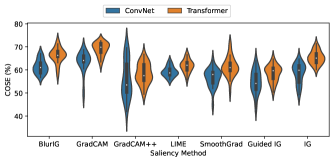
Figure 3: The distributions of COSE for ConvNets and Transformers compared for all saliency methods, shown as a violin plot. Within each violin, the thin line shows the 1.5x interquartile range, the thick line shows the interquartile range, and the white dot shows the median. The shape of the violin shows how data points are distributed. Transformers outperform ConvNets on average for all methods.

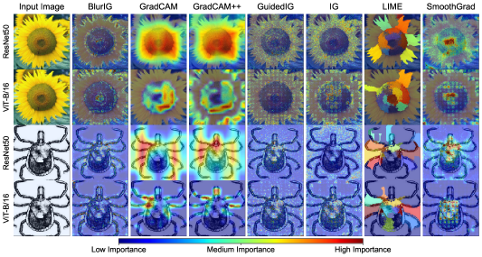
Figure 4: Results of saliency methods on ViT-B/16 (a transformer model), ResNet50 (a convolutional model), and Oxford102/Caltech101. We qualitatively observe the explanations for ViT-B/16 to be similar (Guided IG, SmoothGrad) or better (BlurIG, IG, LIME, GradCAM, GradCAM++). In general, we find transformer model explanations are more coherent than convolutional model explanations.

4.1 Transformers have better explanations

Transformer explanations had higher COSE and sensitivity for all methods. Figure 3 shows transformer model explanations consistently outperforming those of ConvNets. Table 1 supports this even further, with transformers obtaining a higher average COSE score than ConvNets for every dataset and saliency method. Transformers also displayed higher sensitivity than ConvNets for almost every dataset and saliency method. In terms of consistency, although we observed ConvNets outperformed transformers for CAM-based methods and CUB, the difference is negligible when looking at the overall performance. Figure 4 illustrates how explanations appear more coherent for ViT-B/16 than ResNet50.

Transformer vs ConvNet receptive fields could explain the difference in saliency maps. The self-attention mechanism of transformers doing patch-wise operations allow for better interpretability due to the availability of a global view of the image. ConvNets, on the other hand, use local operators that have limited receptive fields, restricting the amount of information that can be utilized by saliency methods [18, 10]. In addition, given unsupervised vision transformers have been found to outperform similarly-trained ConvNets in terms of various segmentation tasks [3], we speculate this better spatial understanding may extend to explanations of vision transformers as well. We explore this further by looking at supervised and unsupervised network comparisons in the appendix.

4.2 GradCAM is more reliable than other methods

GradCAM has the highest COSE for most of the experiments. Table 1 shows the performance of different saliency methods across all datasets and models. In 65% of the evaluation settings, GradCAM outperformed other saliency methods, with BlurIG having the highest COSE for 22.5% of the experiments, IG for 5%, GradCAM++ for 5%, and GuidedIG for 2.5% of the experiments. Although COSE is a descriptive single metric for overall performance, we also look at the performance of saliency methods on consistency and sensitivity individually to give further insight into what contributes to the performance of the saliency methods.

Dataset	Model	BlurIG	GradCAM	GradCAM++	GuidedIG	IG	LIME	SmoothGrad
		[29]	[22]	[4]	[13]	[24]	[21]	[23]
Caltech101	ConvNext	63.01%	63.50%	65.28%	54.25%	62.53%	61.51%	60.90%
	ResNet50	65.77%	61.86%	45.41%	52.41%	58.80%	56.69%	59.60%
	Swin-T	67.81%	67.15%	57.50%	52.54%	64.68%	63.17%	61.95%
	ViT-B/16	69.60%	68.66%	60.30%	57.48%	66.67%	61.12%	66.41%
CIFAR10	ConvNext	61.46%	66.74%	66.72%	53.02%	60.91%	62.06%	58.85%
	ResNet50	60.47%	62.29%	42.75%	48.27%	51.20%	59.86%	52.02%
	Swin-T	66.35%	69.66%	58.29%	50.11%	63.05%	65.76%	56.95%
	ViT-B/16	66.46%	71.54%	59.11%	55.72%	66.68%	63.85%	61.00%
CUB200	ConvNext	54.15%	60.61%	59.81%	59.59%	61.20%	56.90%	47.89%
	ResNet50	58.63%	44.01%	40.74%	56.50%	60.05%	55.50%	52.38%
	Swin-T	62.37%	62.51%	49.78%	60.14%	64.02%	59.06%	56.05%
	ViT-B/16	59.07%	64.80%	56.65%	61.26%	60.42%	58.31%	53.70%
EuroSAT	ConvNext	59.17%	65.47%	63.58%	52.83%	61.45%	60.23%	57.17%
	ResNet50	57.28%	62.27%	45.17%	40.87%	46.14%	59.47%	47.96%
	Swin-T	64.74%	66.49%	53.82%	47.51%	61.99%	59.60%	60.43%
	ViT-B/16	67.85%	70.31%	57.95%	57.90%	68.12%	60.63%	62.48%
Oxford102	ConvNext	58.60%	62.78%	61.74%	58.73%	60.71%	57.23%	57.77%
	ResNet50	61.13%	61.90%	40.30%	54.93%	55.07%	58.32%	56.60%
	Swin-T	66.57%	67.38%	56.87%	52.86%	63.42%	62.06%	59.41%
	ViT-B/16	66.90%	68.31%	59.14%	59.67%	65.92%	61.44%	62.95%
	Overall	63.23%	64.66%	54.59%	54.73%	61.33%	60.11%	57.94%

Table 1: COSE score of different saliency methods on various models and datasets. For each dataset and model combination, the best saliency method is bolded and the second-best is underlined. For most models and datasets, GradCAM has the highest COSE, followed by BlurIG and IG. It can also be seen that most methods (GradCAM, GradCAM++, BlurIG) apart from IG and GuidedIG struggle with CUB200.

GradCAM can reflect changing model behavior. Figure 5 shows the relationship between the model accuracy at a collection of intermediate model training epochs $e$ and the difference in saliency maps $M_{final}$ and $M_{e}$ ($\operatorname{SSIM}(M_{e},M_{final})$). $M_{final}$ is the saliency map for a fully trained model, and $M_{e}$ is the saliency map of an untrained or a partially trained model. Both LIME and GradCAM show a significant positive correlation between SSIM and accuracy, indicating that saliency maps from these methods can illustrate changes in model performance.

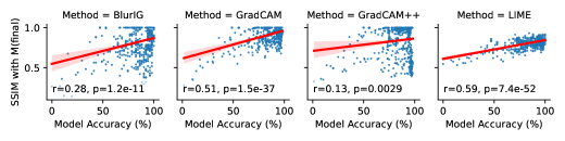
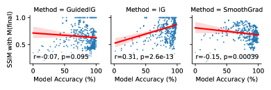
Figure 5: SSIM of the saliency map of the final trained model $M_{final}$ with respect to the saliency map of a partially trained model $M_{e}$. GradCAM and LIME generally has increasing SSIM with increasing model accuracy. The correlation (r) and the corresponding p-values (p) are also annotated in each plot. We use alpha=0.05 (correlation for GuidedIG is insignificant).

GradCAM is more robust to data transformations. Looking at the consistency metrics in Figure 6, GradCAM has the highest average consistency. The general distribution also shows GradCAM having more samples with high consistency values when compared to other methods. This indicates that GradCAM, followed by GradCAM++ and BlurIG, are robust to data transformations that do not affect model behavior.

Limitations of GradCAM. Although GradCAM is shown to do better than other methods for most of the models and datasets, it evidently struggles with CUB200. Table 1 shows the COSE for various saliency methods across datasets and metrics. It also shows GradCAM has low scores on CUB200. Figure 7 shows that across different saliency methods, CUB200 has the lowest average COSE. This could be contributed to the tendency of CAM methods to emphasize larger areas of importance. Unlike GradCAM and GradCAM++, IG and GuidedIG focus on specific details (also see Figure 1 for sample results), and are observed to perform better on CUB200 based on COSE. The ability to distinguish between small differences on fine-grained datasets like CUB200 can significantly affect the performance of a saliency method.

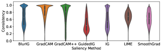
Figure 6: GradCAM has the highest average consistency. We can also observe the distribution of consistency across different samples, with GradCAM having more samples with high consistency.

4.3 How do we improve existing saliency methods?

Balancing consistency and sensitivity. GradCAM is shown to outperform other saliency methods on several angles. However, with a COSE of 64.66%, GradCAM still has areas for improvement. Figure 1 shows that GradCAM tends to predict general areas, which limits its sensitivity to model changes. Due to the large salient area presented, it’s more difficult to isolate differences due to model changes. SmoothGrad and BlurIG show more specific areas, but they tend to be unstable to input perturbations. Future work on saliency methods should aim to balance performance on both - being robust while maintaining good sensitivity.

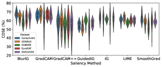
Figure 7: Most saliency methods struggle with CUB200. Looking at each saliency method group, CUB200 has the lowest average performance for all methods except GuidedIG and IG.

Methods should consider both geometric and photometric consistency. Figure 8 shows saliency methods generally have lower consistency and higher sensitivity as transformation magnitudes increase, but ultimately average to a stable COSE over all transformation magnitudes. Splitting into geometric and photometric transformations, we observe in the same figure that this trend is mostly for photometric transformations, as saliency methods perform about the same even when geometric transformations increase. This suggests that saliency methods struggle in different ways for photometric and geometric transformations. While COSE gives an overview of overall performance across all transform magnitudes, we recommend saliency method developers consider photometric changes and geometric changes as separate problems while trying to achieve consistency in both.

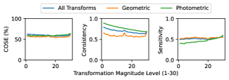
Figure 8: Average performance for all methods on all transformations and separately for geometric and photometric transformations. While photometric transformations have decreasing sensitivity and increasing fidelity as transformation magnitudes increase, geometric transformations seem to have approximately the same performance regardless of transformation magnitude.

5 Conclusion

We presented an evaluation pipeline measuring two crucial characteristics for saliency methods - consistency, which requires images with the same classification to have the same explanation, and sensitivity, which describes that images with different classifications to have different explanations. We combine these two measures into a single metric COSE which is only maximized by balancing the two properties. By applying natural augmentations to images in arbitrary datasets, we show our metrics can emphasize the advantages and the limitations of saliency methods when ground truth model explanations are not available.

Through our metrics, we analyzed the performance of seven commonly used saliency methods across five datasets and eight models. Fundamentally, our metric COSE is best-suited for saliency metrics whose explanations closely reflect the prediction of the network - giving similar explanations for the consistent model behavior and contrasting explanations for different model behavior. We see our work as a starting point for researchers to further explore and improve saliency methods for better model understanding.

Acknowledgements.

The project was funded in part by NSF grant #1749833 to Subhransu Maji. The experiments were performed on the University of Massachusetts GPU cluster funded by the Mass. Technology Collaborative.

References

- [1] Julius Adebayo, Justin Gilmer, Michael Muelly, Ian Goodfellow, Moritz Hardt, and Been Kim. Sanity checks for saliency maps. In Advances in neural information processing systems, volume 31, 2018.
- [2] Julius Adebayo, Michael Muelly, Ilaria Liccardi, and Been Kim. Debugging tests for model explanations. In Advances in Neural Information Processing Systems, volume 33, pages 700–712, 2020.
- [3] Mathilde Caron, Hugo Touvron, Ishan Misra, Hervé Jégou, Julien Mairal, Piotr Bojanowski, and Armand Joulin. Emerging properties in self-supervised vision transformers. In Proceedings of the IEEE/CVF international conference on computer vision, pages 9650–9660, 2021.
- [4] Aditya Chattopadhay, Anirban Sarkar, Prantik Howlader, and Vineeth N Balasubramanian. Grad-cam++: Generalized gradient-based visual explanations for deep convolutional networks. In 2018 IEEE winter conference on applications of computer vision (WACV), pages 839–847. IEEE, 2018.
- [5] Xinlei Chen, Saining Xie, and Kaiming He. An empirical study of training self-supervised vision transformers. In Proceedings of the IEEE/CVF International Conference on Computer Vision, pages 9640–9649, 2021.
- [6] Jia Deng, Wei Dong, Richard Socher, Li-Jia Li, Kai Li, and Li Fei-Fei. Imagenet: A large-scale hierarchical image database. In 2009 IEEE conference on computer vision and pattern recognition, pages 248–255. Ieee, 2009.
- [7] Alexey Dosovitskiy, Lucas Beyer, Alexander Kolesnikov, Dirk Weissenborn, Xiaohua Zhai, Thomas Unterthiner, Mostafa Dehghani, Matthias Minderer, Georg Heigold, Sylvain Gelly, Jakob Uszkoreit, and Neil Houlsby. An image is worth 16x16 words: Transformers for image recognition at scale. International Conference on Learning Representations (ICLR), 2021.
- [8] Thomas Fel, David Vigouroux, Rémi Cadène, and Thomas Serre. How good is your explanation? algorithmic stability measures to assess the quality of explanations for deep neural networks. In Proceedings of the IEEE/CVF Winter Conference on Applications of Computer Vision, pages 720–730, 2022.
- [9] Kaiming He, Xiangyu Zhang, Shaoqing Ren, and Jian Sun. Deep residual learning for image recognition. In Proceedings of the IEEE conference on computer vision and pattern recognition, pages 770–778, 2016.
- [10] Shuting He, Hao Luo, Pichao Wang, Fan Wang, Hao Li, and Wei Jiang. Transreid: Transformer-based object re-identification. In Proceedings of the IEEE/CVF international conference on computer vision, pages 15013–15022, 2021.
- [11] Patrick Helber, Benjamin Bischke, Andreas Dengel, and Damian Borth. Eurosat: A novel dataset and deep learning benchmark for land use and land cover classification. In IEEE Journal of Selected Topics in Applied Earth Observations and Remote Sensing, volume 12, pages 2217–2226. IEEE, 2019.
- [12] Andrei Kapishnikov, Tolga Bolukbasi, Fernanda Viégas, and Michael Terry. Xrai: Better attributions through regions. In Proceedings of the IEEE/CVF International Conference on Computer Vision, pages 4948–4957, 2019.
- [13] Andrei Kapishnikov, Subhashini Venugopalan, Besim Avci, Ben Wedin, Michael Terry, and Tolga Bolukbasi. Guided integrated gradients: An adaptive path method for removing noise. In Proceedings of the IEEE/CVF conference on computer vision and pattern recognition, pages 5050–5058, 2021.
- [14] Alex Krizhevsky, Geoffrey Hinton, et al. Learning multiple layers of features from tiny images. 2009.
- [15] Fei-Fei Li, Marco Andreeto, Marc’Aurelio Ranzato, and Pietro Perona. Caltech 101, Apr 2022.
- [16] Ze Liu, Yutong Lin, Yue Cao, Han Hu, Yixuan Wei, Zheng Zhang, Stephen Lin, and Baining Guo. Swin transformer: Hierarchical vision transformer using shifted windows. In Proceedings of the IEEE/CVF international conference on computer vision, pages 10012–10022, 2021.
- [17] Zhuang Liu, Hanzi Mao, Chao-Yuan Wu, Christoph Feichtenhofer, Trevor Darrell, and Saining Xie. A convnet for the 2020s. In Proceedings of the IEEE/CVF Conference on Computer Vision and Pattern Recognition, pages 11976–11986, 2022.
- [18] Wenjie Luo, Yujia Li, Raquel Urtasun, and Richard Zemel. Understanding the effective receptive field in deep convolutional neural networks. Advances in neural information processing systems, 29, 2016.
- [19] Samuel G Müller and Frank Hutter. Trivialaugment: Tuning-free yet state-of-the-art data augmentation. In Proceedings of the IEEE/CVF international conference on computer vision, pages 774–782, 2021.
- [20] Maria-Elena Nilsback and Andrew Zisserman. Automated flower classification over a large number of classes. In 2008 Sixth Indian Conference on Computer Vision, Graphics & Image Processing, pages 722–729. IEEE, 2008.
- [21] Marco Tulio Ribeiro, Sameer Singh, and Carlos Guestrin. ” why should i trust you?” explaining the predictions of any classifier. In Proceedings of the 22nd ACM SIGKDD international conference on knowledge discovery and data mining, pages 1135–1144, 2016.
- [22] Ramprasaath R Selvaraju, Michael Cogswell, Abhishek Das, Ramakrishna Vedantam, Devi Parikh, and Dhruv Batra. Grad-cam: Visual explanations from deep networks via gradient-based localization. In Proceedings of the IEEE international conference on computer vision, pages 618–626, 2017.
- [23] Daniel Smilkov, Nikhil Thorat, Been Kim, Fernanda Viégas, and Martin Wattenberg. Smoothgrad: removing noise by adding noise. arXiv preprint arXiv:1706.03825, 2017.
- [24] Mukund Sundararajan, Ankur Taly, and Qiqi Yan. Axiomatic attribution for deep networks. In International conference on machine learning, pages 3319–3328. PMLR, 2017.
- [25] Keyu Tian, Yi Jiang, Qishuai Diao, Chen Lin, Liwei Wang, and Zehuan Yuan. Designing bert for convolutional networks: Sparse and hierarchical masked modeling. arXiv:2301.03580, 2023.
- [26] Richard Tomsett, Dan Harborne, Supriyo Chakraborty, Prudhvi Gurram, and Alun Preece. Sanity checks for saliency metrics. In Proceedings of the AAAI conference on artificial intelligence, volume 34, pages 6021–6029, 2020.
- [27] Zhou Wang, Alan C Bovik, Hamid R Sheikh, and Eero P Simoncelli. Image quality assessment: from error visibility to structural similarity. In IEEE transactions on image processing, volume 13, pages 600–612. IEEE, 2004.
- [28] Peter Welinder, Steve Branson, Takeshi Mita, Catherine Wah, Florian Schroff, Serge Belongie, and Pietro Perona. Caltech-ucsd birds 200. 2010.
- [29] Shawn Xu, Subhashini Venugopalan, and Mukund Sundararajan. Attribution in scale and space. In Proceedings of the IEEE/CVF Conference on Computer Vision and Pattern Recognition, pages 9680–9689, 2020.
- [30] Mengjiao Yang and Been Kim. Benchmarking attribution methods with relative feature importance. arXiv preprint arXiv:1907.09701, 2019.
- [31] Chih-Kuan Yeh, Cheng-Yu Hsieh, Arun Suggala, David I Inouye, and Pradeep K Ravikumar. On the (in) fidelity and sensitivity of explanations. In Advances in Neural Information Processing Systems, volume 32, 2019.
- [32] Bolei Zhou, Aditya Khosla, Agata Lapedriza, Aude Oliva, and Antonio Torralba. Learning deep features for discriminative localization. In Proceedings of the IEEE conference on computer vision and pattern recognition, pages 2921–2929, 2016.
- [33] Jianlong Zhou, Amir H Gandomi, Fang Chen, and Andreas Holzinger. Evaluating the quality of machine learning explanations: A survey on methods and metrics. In Electronics, volume 10, page 593. MDPI, 2021.
- [34] Jinghao Zhou, Chen Wei, Huiyu Wang, Wei Shen, Cihang Xie, Alan Yuille, and Tao Kong. ibot: Image bert pre-training with online tokenizer. International Conference on Learning Representations (ICLR), 2022.
- [35] Yilun Zhou, Serena Booth, Marco Tulio Ribeiro, and Julie Shah. Do feature attribution methods correctly attribute features? In Proceedings of the AAAI Conference on Artificial Intelligence, volume 36, pages 9623–9633, 2022.
- [36] Roland S Zimmermann, Judy Borowski, Robert Geirhos, Matthias Bethge, Thomas Wallis, and Wieland Brendel. How well do feature visualizations support causal understanding of cnn activations? In Advances in Neural Information Processing Systems, volume 34, pages 11730–11744, 2021.