SpikingNeRF: Making Bio-inspired Neural Networks See through the Real World

Abstract

Spiking neural networks (SNNs) have been thriving on numerous tasks to leverage their promising energy efficiency and exploit their potentialities as biologically plausible intelligence. Meanwhile, the Neural Radiance Fields (NeRF) render high-quality 3D scenes with massive energy consumption, but few works delve into the energy-saving solution with a bio-inspired approach. In this paper, we propose SpikingNeRF, which aligns the radiance ray with the temporal dimension of SNN, to naturally accommodate the SNN to the reconstruction of radiance fields. Thus, the computation turns into a spike-based, multiplication-free manner, reducing the energy consumption. In SpikingNeRF, each sampled point on the ray is matched to a particular time step, and represented in a hybrid manner where the voxel grids are maintained as well. Based on the voxel grids, sampled points are determined whether to be masked for better training and inference. However, this operation also incurs irregular temporal length. We propose the temporal padding strategy to tackle the masked samples to maintain regular temporal length, i.e., regular tensors, and the temporal condensing strategy to form a denser data structure for hardware-friendly computation. Extensive experiments on a variety of datasets demonstrate that our method reduces the 70.79% energy consumption on average and obtains comparable synthesis quality with the ANN baseline.

1 Introduction

Spiking neural network (SNN) is considered the third generation of the neural network, and its bionic modeling encourages much research attention to explore the prospective biological intelligence that features multi-task supporting as the human brain does[27, 35]. While, much dedication has been devoted to SNN research, the gap between the expectation of SNN boosting a wider range of intelligent tasks and the fact of artificial neural networks (ANN) dominating deep learning in the majority of tasks still exists.

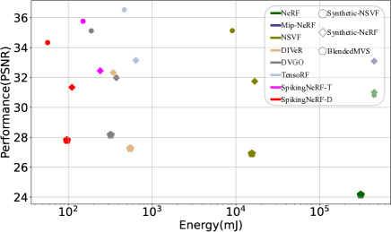
Figure 1: Comparisons of our SpikingNeRF with other NeRF-based works in synthesis quality and model rendering energy. Different colors represent different works, and our works with two different frameworks are denoted in red and violet, respectively. Detailed notation explanation is specified in Sec. 5. Different testing datasets are denoted in different shapes.

Recently, more research interests have been invested to shrink the gap and acquired notable achievements in various tasks, including image classification[49], object detection[46], graph prediction[52], natural language processing[51], etc. Despite multi-task supporting, SNN research is also thriving in performance lifting and energy efficiency exploration at the same time. However, we have not yet witnessed the establishment of SNN in the real 3D reconstruction task with an advanced performance. To this end, this naturally raises an issue: could bio-inspired spiking neural networks reconstruct the real 3D scene with an advanced quality at low energy consumption? In this paper, we investigate the rendering of neural radiance fields with a spiking approach to answer this question.

We propose SpikingNeRF to reconstruct a volumetric scene representation from a set of images. Learning from the huge success of NeRF[31] and its follow-ups[2, 3, 33, 34, 37], we utilize the voxel grids and the spiking multilayer perceptron (sMLP) to jointly model the volumetric representations. In such hybrid representations, voxel grids explicitly store the volumetric parameters, and the spiking multilayer perceptron (sMLP) implicitly transforms the parameters into volumetric information, i.e., the density and color information of the radiance fields. After the whole model is established, we follow the classic ray-sample accumulation method of radiance fields to render the colors of novel scenes[29]. To accelerate the training and inference, we use the voxel grids to predefine borders and free space, and mask those samples out of borders, in free space or with a low-density value as proposed in [37].

Inspired by the imaging process of the primate fovea in the retina that accumulates the intensity flow over time to stimulate the photoreceptor cell[28, 39], we associate the accumulation process of rendering with the temporal accumulation process of SNNs, which ultimately stimulates the spiking neurons to fire. Guided by the above insight, we align the ray with the temporal dimension of the sMLP, and match each sampled point on the ray to a time step one-to-one during rendering. Therefore, different from the original rendering process where all sampled points are queried separately to retrieve the corresponding volumetric information, sampled points are queried sequentially along each ray in SpikingNeRF, and the geometric consecutiveness of the ray is thus transformed into the temporal continuity of the SNN. As a result, SpikingNeRF seizes the nature of both worlds to make the NeRF rendering in a spiking manner.

However, the number of sampled points on different rays varies due to the aforementioned masking operation, which causes the temporal lengths of different rays to become irregular. Consequently, the querying for the color information can hardly be parallelized on graphics processing units (GPUs), severely hindering the rendering process. To solve this issue, we first investigate the temporal padding (TP) method to attain the regular temporal length in a querying batch, i.e., a regular-shaped tensor, thus ensuring parallelism. Furthermore, we propose the temporal condensing-and-padding (TCP), which totally removes the temporal effect of masked points, to fully constrain the tensor size and condense the data distribution, which is hardware-friendly to domain-specific accelerators. Our thorough experimentation proves that TCP can maintain the energy merits and good performance of SpikingNeRF as shown in Fig. 1.

To sum up, our main contributions are as follows:

• We propose SpikingNeRF that aligns the radiance rays in NeRF with the temporal dimension of SNNs. To the best of our knowledge, this is the first work to accommodate spiking neural networks to reconstructing real 3D scenes.

• We propose TP and TCP to solve the irregular temporal lengths, ensuring the training and inference parallelism on GPUs and keeping hardware-friendly.

• Our experiments demonstrate the effectiveness of SpikingNeRF on four mainstream inward-facing 3D reconstruction tasks, achieving advanced energy efficiency as shown in Fig. 1. For another specific example, SpikingNeRF-D can reduce 72.95% rendering energy consumption with 0.33 PSNR drop on Tanks&Temples.

2 Related work

NeRF-based 3D reconstruction.

Different from the traditional 3D reconstruction methods that mainly rely on the explicit and discrete volumetric representations, NeRF[31] utilizes a coordinate neural network to implicitly represent the 3D radiance field, and synthesizes novel views by accumulating the density and color information along the view-dependent rays with the ray tracing algorithm[17]. With this new paradigm of 3D reconstruction, NeRF achieves huge success in improving the quality of novel view synthesis. The followup works further enhance the rendering quality[6, 1, 38], and many others focus on accelerating the training[7, 12, 37] or rendering process[24, 34, 45, 37]. While, we concentrate on exploring the potential integration of the spike-based low-energy communication and NeRF-based high-quality 3D synthesis, seeking ways to the energy-efficient real 3D reconstruction.
Fast NeRF synthesis. The accumulation process of rendering in NeRF[31] requires a huge number of MLP querying, which incurs heavy flop-operation and memory-access burdens, delaying the synthesis speed. Recent studies further combine the traditional explicit volumetric representations, e.g., voxels[15, 26, 37] and MPIs[40], with MLP-dependent implicit representations to obtain more efficient volumetric representations. Thus, the redundant MLP queries for points in free space can be avoided. In SpikingNeRF, we adopt the voxel grids to mask the irrelevant points with low density, and discard unimportant points with low weights, thus reducing the synthesis overhead.
Spiking neural networks. With the high sparsity and multiplication-free operation, SNNs outstrip ANNs in the competition of energy efficiency[5, 23, 21], but fall behind in the performance lifting. Therefore, great efforts have been dedicated to making SNNs deeper[48, 10], converge faster[42, 8], and eventually high-performance[49]. With the merits of energy efficiency and advanced performance, recent SNN research sheds light on exploring versatile SNNs, e.g., Spikeformer[49], Spiking GCN[52], SpikeGPT[51]. In this paper, we seize the analogous nature of both NeRF and SNNs to make bio-inspired spiking neural networks reconstruct the real 3D scene with an advanced quality at low energy consumption.
SNNs in 3D reconstruction. Applying SNNs to 3D Reconstruction has been researched with very limited efforts. As far as we know, only two works exist in this scope. EVSNN [50] is the first attempt to develop a deep SNN for image reconstruction task, which achieves comparable performance to ANN. E2P [30] strives to solve the event-to-polarization problem and uses SNNs to achieve a better polarization reconstruction performance. Unfortunately, both of them focus solely on the reconstruction of event-based images with traditional methods, neglecting the rich RGB world. While, we are the first to explore the reconstruction of the real RGB world with SNNs.

3 Preliminaries

Neural radiance field. To reconstruct the scene for the given view, NeRF[31] first utilizes an MLP, which takes in the location coordinate $\mathbf{p}\in\mathbb{R}^{3}$ and the view direction $\mathbf{v}\in\mathbb{R}^{2}$ and yields the density $\sigma\in\mathbb{R}$ and the color $\mathbf{c}\in\mathbb{R}^{3}$, to implicitly maintain continuous volumetric representations:

$$\mathbf{e},\sigma =MLP_{\theta}(\mathbf{p}),$$ (1)

$$\mathbf{c} =MLP_{\gamma}(\mathbf{e},\mathbf{v}),$$ (2)

where $\theta$ and $\gamma$ denote the parameters of the separate two parts of the MLP, and $\mathbf{e}$ is the embedded features. Next, NeRF renders the pixel of the expected scene by casting a ray $\mathbf{r}$ from the camera origin point to the direction of the pixel, then sampling $K$ points along the ray. Through querying the MLP as in Eq. (1-2) $K$ times, $K$ color values and $K$ density values can be retrieved. Finally, following the principles of the discrete volume rendering proposed in [29], the expected pixel RGB $\hat{C}(\mathbf{r})$ can be rendered:

$$\alpha=1-\exp(-\sigma_{i} \delta_{i}),\quad T_{i}=\prod^{i-1}_{j=1}(1-\alpha_{i}),$$ (3)

$$\hat{C}(\mathbf{r}) \approx\sum^{K}_{i=1}T_{i}\alpha_{i}\mathbf{c}_{i},$$ (4)

where $\mathbf{c}_{i}$ and $\sigma_{i}$ denotes the color and the density values of the $i$-th point respectively, and $\delta_{i}$ is the distance between the adjacent point $i$ and $i+1$.

After rendering all the pixels, the expected scene is reconstructed. With the ground-truth pixel color $C(\mathbf{r})$, the parameters of the MLP can be trained end-to-end by minimizing the MSE loss:

$$\mathcal{L}=\frac{1}{|\mathcal{R}|}\sum_{r\in\mathcal{R}}\|\hat{C}(\mathbf{r})-C(\mathbf{r})\|^{2}_{2},$$ (5)

where $\mathcal{R}$ is the mini-batch containing the sampled rays.
Hybrid volumetric representation. The number of sampled points $K$ in Eq. 4 is usually big, leading to the heavy MLP querying burden as displayed in Eq. (1-2). To alleviate this problem, voxel grid representation is utilized to contain the volumetric parameters directly, e.g., the embedded feature $e$ and the density $\sigma$ in Eq. 1, as the values of the voxel grid. Thus, querying the MLP in Eq. 1 is substituted to querying the voxel grids and operating the interpolation, which is much easier:

$$\sigma=\mathrm{act}(\mathrm{interp}(\mathbf{p},\mathbf{V_{\sigma}})),$$ (6)

$$\mathbf{e}=\mathrm{interp}(\mathbf{p},\mathbf{V_{f}}),$$ (7)

where $\mathbf{V_{\sigma}}$ and $\mathbf{V_{f}}$ are the voxel grids related to the volumetric density and features, respectively. “interp” denotes the interpolation operation, and “act” refers to the activation function, e.g., ReLU or the shifted softplus[1].

Furthermore, those irrelevant points with low density or unimportant points with low weight can be masked through predefined thresholds $\lambda$, then Eq. 4 turns into:

$$A\triangleq\{i:T_{i}>\lambda_{1},\alpha_{i}>\lambda_{2}\},$$ (8)

$$\hat{C}(\mathbf{r})\approx\sum_{i\in A}T_{i}\alpha_{i}\mathbf{c}_{i}.$$ (9)

Thus, the queries of the MLP for sampled points in Eq. 2 are significantly reduced.
Spiking neuron. The spiking neuron is the most fundamental unit in spiking neural networks, which essentially differs SNNs from ANNs. The modeling of spiking neuron commonly adopts the leaky integrate-and-fire (LIF) model:

$$\mathbf{U}^{t} =\mathbf{V}^{t-1}+\frac{1}{\tau}(\mathbf{X}^{t}-\mathbf{V}^{t-1}+V_{reset}),$$ (10)

$$\mathbf{S}^{t} =\mathbb{H}(\mathbf{U}^{t}-V_{th}),$$ (11)

$$\mathbf{V}^{t} =\mathbf{U}^{t}\odot(1-\mathbf{S}^{t})+V_{reset}\mathbf{S}^{t}.$$ (12)

Here, $\odot$ denotes the Hadamard product. $\mathbf{U}^{t}$ is the intermediate membrane potential at time-step $t$ and can be updated through Eq. 10, where $\mathbf{V}^{t-1}$ is the actual membrane potential at time-step $t-1$ and $\mathbf{X}^{t}$ denotes the input vector at time-step $t$, e.g., the activation vector from the previous layer in MLPs. The output spike vector $\mathbf{S}^{t}$ is given by the Heaviside step function $\mathbb{H}(\cdot)$ in Eq. 11, indicating that a spike is fired when the membrane potential exceeds the potential threshold $V_{th}$. Dependent on whether the spike is fired at time-step $t$, the membrane potential $\mathbf{V}^{t}$ is set to $\mathbf{U}^{t}$ or the reset potential $V_{reset}$ through Eq. 12.

Since the Heaviside step function $\mathbb{H}(\cdot)$ is not differentiable, the surrogate gradient method is utilized to solve this issue, which is defined as :

$$\frac{d\mathbb{H}(x)}{dx}=\frac{1}{1+\exp(-\alpha x)},$$ (13)

where $\alpha$ is a predefined hyperparameter. Thus, spiking neural networks can be optimized end-to-end.

4 Methodology

4.1 Data encoding

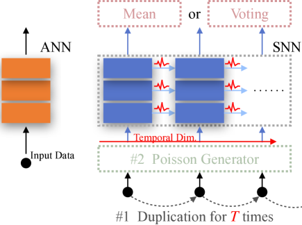
Figure 2: Conventional data encoding schemes. For direct-encoding, the operation #1 is necessary that the input data will be duplicated $T$ times to fit the length of the temporal dimension. For Poisson-encoding, both operation #1 and #2 are utilized to generate the input spike train. The “Mean” or “Voting” operation is able to decoding the SNN output.

In this subsection, we explore two naive data encoding approaches for converting the input data to SNN-tailored formats, i.e., direct-encoding and Poisson-encoding. Both of them are proven performing well in the direct learning of SNNs[11, 22, 14, 36, 4].

As described in Sec. 3, spiking neurons receive data with an additional dimension called the temporal dimension, which is indexed by the time-step $t$ in Eq. (10-12). Consequently, original ANN-formatted data need to be encoded to fill the temporal dimension as illustrated in Fig. 2. In the direct-encoding scheme, the original data is duplicated $T$ times to fill the temporal dimension, where $T$ represents the total length of the temporal dimension. As for the Poisson-encoding scheme, besides the duplication operation, it perceives the input value as the probability and generates a spike according to the probability at each time step. Additionally, a decoding method is entailed for the subsequent operations of rendering, and the mean [22] and the voting[11] decoding operations are commonly considered. We employ the former approach since the latter one is designed for classification tasks[9, 42].

Thus, with the above two encoding methods, we build two naive versions of SpikingNeRF, and conduct experiments on various datasets to verify the feasibility.

4.2 Time-ray alignment

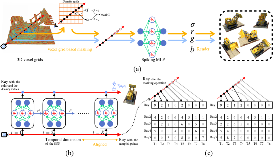
Figure 3: Overview of the proposed SpikingNeRF. (a) The rendering process of SpikingNeRF. The whole 3D volumetric parameters are stored in the voxel grids. The irrelevant or unimportant samples are masked before the sMLP querying. The expected scenes are rendered with the volumetric information yielded by the sMLP. (b) Alignment between the temporal dimension and the ray. The sMLP queries each sampled point step-by-step to yield the volumetric information. (c) Proposed temporal padding (left) and temporal condensing-and-padding (right) methods. For simplification, the channel length of the volumetric parameters is set to 1.

This subsection further explores the potential of accommodating the SNN to the NeRF rendering process in a more natural and novel way, where we attempt to remain the real-valued input data as direct-encoding does, but do not fill the temporal dimension with the duplication-based approach.

We first consider the MLP querying process in the ANN philosophy. For an expected scene to reconstruct, the volumetric parameters of sampled points, e.g., $e$ and $v$ in Eq. 2, are packed as the input data with the shape of $[batch,c_{e}]$ or $[batch,c_{v}]$, where $batch$ represents the sample index and $c$ is the channel index of the volumetric parameters. Thus, the MLP can query these data and output the corresponding color information in parallel. However, from the geometric view, the input data should be packed as $[ray,pts,c]$, where $ray$ is the ray index and the $pts$ is the index of the sampled points.

Obviously, the ANN-based MLP querying process can not reflect such geometric relations between the ray and the sampled points. Then, we consider the computation modality of SNNs. As illustrated in Eq. (10-12), SNNs naturally entail the temporal dimension to process the sequential signals. This means a spiking MLP naturally accepts the input data with the shape of $[batch,time,c]$, where $time$ is the temporal index. Therefore, we can reshape the volumetric parameters back to $[ray,pts,c]$, and intuitively match each sample along the ray to the corresponding time step:

$$\begin{split}\text{Input}_{MLP}&:=[batch,c]\\ &\Rightarrow[ray,pts,c]\\ &\Rightarrow[batch,time,c]:=\text{Input}_{sMLP},\end{split}$$ (14)

which is also illustrated in Fig. 3(b). Such an alignment does not require any input data pre-process such as duplication[49] or Poisson generation[13] as prior arts commonly do.

4.3 TCP

Yet the masking operation on sampled points, as illustrated in Sec. 3, makes the time-ray alignment intractable. Although such masking operation improves the rendering speed and quality by curtailing the computation cost of redundant samples, it also causes the number of queried samples on different rays to be irregular, which indicates the reshape operation of Eq. 14, i.e., shaping into a tensor, is unfeasible on GPUs after the masking operation.

To ensure computation parallelism on GPUs, we first propose to retain the indices of those masked samples but discard their values. As illustrated in Fig. 3(c) Left, we arrange both unmasked and masked samples sequentially to the corresponding $ray$-indexed vector, and pad zeros to the vacant tensor elements. Such that, a regular-shaped input tensor is built. We refer to this simple approach as the temporal padding (TP) method.

However, TP does not handle those masked samples effectively because those padded zeros will still get involved in the following computation and cause the membrane potential of sMLP to decay, implicitly affecting the outcomes of the unmasked samples in the posterior segment of the ray. Even for a sophisticated hardware accelerator that can skip those zeros, the sparse data structure still causes computation inefficiency such as imbalanced workload[47]. To solve this issue, we design the temporal condensing-and-padding (TCP) scheme, which is illustrated in Fig. 3(c) Right. Different from TP, TCP completely discards the parameters and indices of the masked samples, and adjacently rearranges the unmasked sampled points to the corresponding $ray$ vector. For the vacant tensor elements, zeros are filled as TP does. Consequently, valid data is condensed to the left side of the tensor. Notably, the $ray$ dimension can be sorted according to the valid data number to further increase the density. As a result, TCP has fully eliminated the impact of the masked samples and made SpikingNeRF more hardware-friendly. Therefore, we choose TCP as our mainly proposed method for the following study.

4.4 Temporal flip

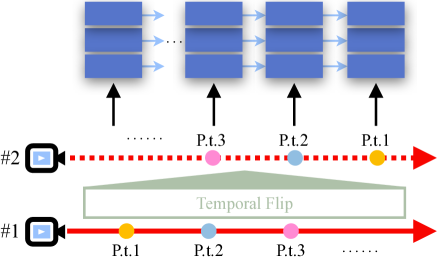
Figure 4: Temporal flip. The direction of the temporal dimension is consistent with the ray #1 but opposite to the ray #2. “P.t.” is the abbreviation of “point”.

Moreover, with the alignment between the temporal dimension and the camera ray, the samples on the same ray are queried by the sMLP sequentially rather than in parallel. This raises an issue: which querying direction is better for SpikingNeRF, the camera ray direction or the opposite one?

In this work, we propose to rely on empirical experiments to choose the querying direction. As illustrated in Fig. 4, the temporal flip operation is utilized to make the directions of the temporal dimension and the camera ray become opposite. The experimental results in Sec. 5.3 indicate the direction of the camera ray is better for SpikingNeRF. Therefore, we choose this direction as our main method.

4.5 Overall algorithm

This section summarizes the overall algorithm of SpikingNeRF based on the DVGO[37] framework. And, the pseudo code is given in Algorithm 1.

As illustrated in Fig. 3(a), SpikingNeRF first establishes the voxel grids filled with learnable volumetric parameters. In the case of the DVGO implementation, two groups of voxel grids are built as the input of Algorithm 1, which are the density and the feature voxel grids. Given an expected scene with $N$ pixels to render, Step 1 is to sample $M$ points along each ray shot from the camera origin to the direction of each pixel. With the $N\times M$ sampled points, Step 2 queries the density grids to compute the weight coefficients, and Step 3 uses these coefficients to mask those irrelevant points. Then, Step 4 queries the feature grids for the filtered points and returns each point’s volumetric parameters. Step 5 and 6 prepare the volumetric parameters into a receivable data format for $sMLP$ with TP or TCP. Step 7 and 8 compute the RGB values for the expected scene. If a backward process is required, Step 9 calculates the MSE loss between the expected and the ground-truth scenes.

Notably, the proposed methods can also be applied to other voxel-grid based NeRF frameworks, e.g., TensoRF[2], NSVF[25], since the core idea is to replace the MLP with the sMLP and exploit the proposed TCP approach. Therefore, we also implement SpikingNeRF on TensoRF for further verification, and defer the corresponding implementation details to the appendix.

Algorithm 1 Overall algorithm of the DVGO-based SpikingNeRF (SpikingNeRF-D) in the rendering process.

0:  The density and the feature voxel grids $V_{\sigma}$ and $V_{f}$, the spiking MLP $sMLP(\cdot)$, the view direction of the camera $v$, the rays from the camera origin to the directions of $N$ pixels of the expected scene $R_{\{N\}}=\{r_{1},r_{2},...,r_{N}\}$, the number of the sampled points per ray $M$, the ground-truth RGB $\mathbf{C}=\{C_{1},C_{2},...,C_{N}\}$ of the expected $N$ pixels .

0:  The expected RGB $\mathbf{\hat{C}}=\{\hat{C}_{1},\hat{C}_{2},...,\hat{C}_{N}\}$ of the expected $N$ pixels, the training loss $\mathcal{L}$.

1:  The location coordinates of the sampled points $P_{\{N\times M\}}=\{p_{1,1},p_{1,2},...,p_{N,M}\}\leftarrow Sample(R)$.

2:  $\alpha_{\{N\times M\}},T_{\{N\times M\}}\leftarrow Weigh(P,V_{\sigma})$ as in Eq. 6 and (3).

3:  Filtered coordinates $P^{\prime}\leftarrow Mask(P,\alpha,T)$ as in Eq. 8.

4:  Input_MLP $\leftarrow QueryFeatures(P^{\prime},V_{f},v)$ as described in Eq. 7 and (2).

5:  The temporal length $T\leftarrow$ The maximum point number among the batched rays.

6:  Input_sMLP $\leftarrow$ The TP or TCP transformation on Input_MLP as described in Sec. 4.3 and Eq. 14.

7:  The RGB values $c_{\{N,T\}}\leftarrow sMLP(\text{Input}_{sMLP})$

8:  $\mathbf{\hat{C}}\leftarrow Accumulate(P^{\prime},\alpha,T,c)$ as in Eq. 9.

9:  $\mathcal{L}\leftarrow MSE(\mathbf{C},\mathbf{\hat{C}})$ as in Eq. 5

Note: Dependent on the specific NeRF framework, the functions, e.g., $Sample(\cdot)$, $Mask(\cdot)$, may be different.

5 Experiments

In this section, we demonstrate the effectiveness of our proposed SpikingNeRF. We first build the codes on the voxel-grid based DVGO framework[37]. Secondly, we compare the proposed SpikingNeRF with the original DVGO method along with other NeRF-based works in both rendering quality and energy cost. Then, we conduct ablation studies to evaluate different aspects of our proposed methods. Finally, we extend SpikingNeRF to other 3D tasks, including unbounded inward-facing and forward-facing datasets, and to the TensoRF framework[2]. The extension results on other 3D tasks are deferred to the appendix. For clarity, we term the DVGO-based SpikingNeRF as SpikingNeRF-D and the TensoRF-based as SpikingNeRF-T.

Table 1: Comparisons with the ANN counterpart and other NeRF-based methods.

Dataset	Synthetic-NeRF			Synthetic-NSVF			BlendedMVS			Tanks&Temples
Metric	PSNR$\uparrow$	SSIM$\uparrow$	Energy$\downarrow$ (mJ)	PSNR$\uparrow$	SSIM$\uparrow$	Energy$\downarrow$ (mJ)	PSNR$\uparrow$	SSIM$\uparrow$	Energy$\downarrow$ (mJ)	PSNR$\uparrow$	SSIM$\uparrow$	Energy$\downarrow$ (mJ)
NeRF[31]	31.01	0.947	4.5e5	30.81	0.952	4.5e5	24.15	0.828	3.1e5	25.78	0.864	1.4e6
Mip-NeRF[1]	33.09	0.961	4.5e5	-	-	-	-	-	-	-	-	-
JaxNeRF[6]	31.65	0.952	4.5e5	-	-	-	-	-	-	27.94	0.904	1.4e6
NSVF[25]	31.74	0.953	16801	35.13	0.979	9066	26.90	0.898	15494	28.40	0.900	103753
DIVeR[41]	32.32	0.960	343.96	-	-	-	27.25	0.910	548.65	28.18	0.912	1930.67
DVGO*[37]	31.98	0.957	374.72	35.12	0.976	187.85	28.15	0.922	320.66	28.42	0.912	2147.86
TensoRF*[2]	33.14	0.963	641.17	36.74	0.982	465.09	-	-	-	28.50	0.920	2790.03
SpikingNeRF-D	31.34	0.949	110.80	34.33	0.970	56.69	27.80	0.912	96.37	28.09	0.896	581.04
SpikingNeRF-T	32.45	0.956	240.81	35.76	0.978	149.98	-	-	-	28.09	0.904	1165.90

• * denotes an ANN counterpart implemented by the official codes.

Table 2: Ablation study with the naive versions.

Dataset	Synthetic-NeRF			Synthetic-NSVF			BlendedMVS			Tanks&Temples
Metric	PSNR$\uparrow$	SSIM$\uparrow$	Energy$\downarrow$ (mJ)	PSNR$\uparrow$	SSIM$\uparrow$	Energy$\downarrow$ (mJ)	PSNR$\uparrow$	SSIM$\uparrow$	Energy$\downarrow$ (mJ)	PSNR$\uparrow$	SSIM$\uparrow$	Energy$\downarrow$ (mJ)
SpikingNeRF-D with time-step 1.
Direct	31.22	0.947	113.03	34.17	0.969	53.73	27.78	0.911	92.70	27.94	0.893	446.31
Poisson	22.03	0.854	49.61	24.83	0.893	29.64	20.74	0.759	58.04	21.53	0.810	377.92
TRA	31.34	0.949	110.80	34.33	0.970	56.69	27.80	0.912	96.37	28.09	0.896	581.04
SpikingNeRF-D with time-step 2.
Direct	31.51	0.951	212.20	34.49	0.971	104.05	27.90	0.915	172.26	28.21	0.900	1076.82
Poisson	21.98	0.855	91.97	24.83	0.893	55.58	20.74	0.759	107.77	21.57	0.814	712.24
TRA	31.34	0.949	110.80	34.33	0.970	56.69	27.80	0.912	96.37	28.09	0.896	581.04
SpikingNeRF-D with time-step 4.
Direct	31.55	0.951	436.32	34.56	0.971	217.86	27.98	0.917	358.82	28.23	0.901	2296.22
Poisson	21.90	0.856	147.49	24.83	0.893	94.36	20.74	0.759	184.82	21.60	0.818	1138.89
TRA	31.34	0.949	110.80	34.33	0.970	56.69	27.80	0.912	96.37	28.09	0.896	581.04

• TRA denotes the time-ray alignment with TCP.

Table 3: Comparisons between TCP and TP.

Dataset	Synthetic-NeRF		Synthetic-NSVF		BlendedMVS		Tanks&Temples
SpikingNeRF-D	w/ TCP	w/ TP	w/ TCP	w/ TP	w/ TCP	w/ TP	w/ TCP	w/ TP
PSNR$\uparrow$	31.34	31.34	34.34	34.33	27.80	27.80	28.09	28.01
Latency(s)	26.12	222.22	13.37	164.61	22.70	243.93	138.98	980.28
Energy+(mJ)	65.78	559.45	33.68	414.37	57.16	614.13	350.03	2468.16

• $+$ denotes the energy result particularly produced by SpikeSim.

Table 4: Comparisons with temporal flip.

Dataset	Synthetic-NeRF		Synthetic-NSVF		BlendedMVS		Tanks&Temples
SpikingNeRF-D	w/o TF	w/ TF	w/o TF	w/ TF	w/o TF	w/ TF	w/o TF	w/ TF
PSNR$\uparrow$	31.34	31.25	34.34	34.15	27.80	27.79	28.09	28.05
SSIM$\uparrow$	0.949	0.947	0.970	0.967	0.912	0.910	0.896	0.894
Energy (mJ)	110.80	116.91	56.69	61.08	96.37	104.75	581.04	612.66

• TF denotes temporal flip.

5.1 Experiments settings

We conduct experiments mainly on the four inward-facing datasets, including Synthetic-NeRF[31] that contains eight objects synthesized from realistic images, Synthetic-NSVF[25] that contains eight objects synthesized by NSVF, BlendedMVS[44] with authentic ambient lighting by blending real images, and Tanks&Temples datasets[18] which is a real world dataset. We refer to DVGO as the ANN counterpart to SpikingNeRF-D, and keep all the hyper-parameters consistent with the original DVGO implementation[37] except for the training iteration in the fine stage being set to 40000. The grid resolutions for all the above datasets are set to $160^{3}$. We also refer to TensoRF as the ANN counterpart to SpikingNeRF-T. In terms of the energy computation, we follow the prior arts[49, 43, 19, 20, 16] to estimate the theoretical rendering energy cost in the most of our experiments except for those in Tab. 3 whose results are produced by SpikeSim[32]. More details about SpikingNeRF-T and the SpikeSim evaluation are specified in the appendix.

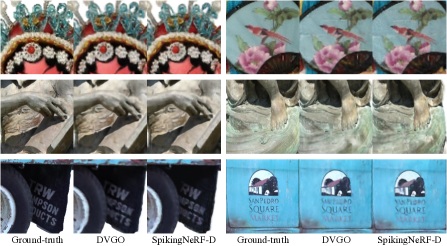
Figure 5: Qualitative comparisons on the different challenging parts. Top: On Character from BlendedMVS, where the color changes densely and intensely. Middle: On Ignatius from Tanks&Temples, where the textures are distinct and dense. Bottom: On Truck from Tanks&Temples, where detail information are explicitly displayed.

5.2 Comparisons

Quantitative evaluation on the synthesized novel view. As shown in Tab. 1, our SpikingNeRF-D can achieve 70.79$\pm$1.2% energy saving with 0.53$\pm$0.19 PSNR drop on average over the ANN counterpart. Such a trade-off between synthesis quality and energy cost is reasonable because a significant part of inference is conducted with the addition operations in the sMLP of SpikingNeRF-D rather than the float-point operations in the original DVGO. On the one hand, compared with those methods[31, 1, 6] that do not perform the masking operation, SpikingNeRF-D can reach orders of magnitude lower energy consumption. On the other hand, compared with those methods[25, 41, 37, 2] that significantly exploit the masking operation, SpikingNeRF-D can still obtain better energy efficiency and comparable synthesis quality. Moreover, SpikingNeRF-T also reduces 62.80$\pm$3.9% energy consumption with 0.69$\pm$0.23 PSNR drop on average. Notably, SpikingNeRF-T only uses two FC layers as TensoRF does. One layer is for encoding data with full precision, the other for spiking with binary computation, leading to only half of the computation burden is tackled with addition operation. This accounts for the reason why SpikingNeRF-T performs a little worse than SpikingNeRF-D on energy reduction ratio. In conclusion, these results demonstrate the effectiveness of our proposed SpikingNeRF in improving energy efficiency.
Qualitative comparisons. Fig. 5 compares SpikingNeRF-D with its ANN counterpart on three different scenes. Basically, SpikingNeRF-D shares the analogous issues with the ANN counterpart on texture distortion and blur.

5.3 Ablation study

Feasibility of the conventional data encodings. As described in Sec. 4.1, we propose two naive versions of SpikingNeRF-D that adopt two different data encoding schemes: direct-encoding and Poisson-encoding. Tab. 2 lists the experimental results. On the one hand, direct-encoding obtains good synthesis performance with only one time step, and can achieve higher PSNR as the time step increases. But, the energy cost also grows linearly with the time step. On the other hand, Poisson-encoding achieves lower energy cost, but the synthesis quality is far from acceptance. The results indicates the direct-encoding shows good feasibility in accommodating SNNs to the NeRF-based rendering.
Effectiveness of the time-ray alignment. To demonstrate the effectiveness of the proposed time-ray alignment, we further compare SpikingNeRF-D with the direct-encoding. In Tab. 2, SpikingNeRF-D can achieve the same-level energy cost as the direct-encoding with time-step 1, while the synthesis quality is consistently better across all the four datasets, which indicates SpikingNeRF is a better trade-off between energy consumption and synthesis performances.
Advantages of temporal condensing. To demonstrate the advantages of the proposed temporal condensing on hardware accelerators as described in Sec. 4.3, we evaluate TCP and TP on SpikeSim with the SpikeFlow architecture. As listed in Tab. 3, TCP consistently outperforms TP in both inference latency and energy overhead by a significant margin over the four datasets. Specifically, on Synthetic-NSVF and BlendedMVS, the gap between TCP and TP is at least an order of magnitude in both inference speed and energy cost. These results demonstrate the effectiveness of a denser data structure in improving computation efficiency on hardware accelerators.
Importance of the alignment direction. As described in Sec. 4.4, we propose temporal flip to empirically decide the alignment direction since the querying direction of sMLP along the camera ray will affect the inference outcome. Tab. 4 lists the experimental results of SpikingNeRF-D with and without temporal flip, i.e., with the consistent and the opposite directions. Distinctly, keeping the direction of the temporal dimension consistent with that of the camera ray outperforms the opposite case over all the four datasets in synthesis performance and energy efficiency. Similar conclusion can also be drawn from the experiments of the TP-based SpikingNeRF-D as shown in the appendix. Therefore, the consistent alignment direction is important in SpikingNeRF.

6 Conclusion

In this paper, we propose SpikingNeRF that accommodates the spiking neural network to reconstructing real 3D scenes for the first time to improve the energy efficiency. In SpikingNeRF, we adopt the direct-encoding that directly inputs the volumetric parameters into SNNs, and align the temporal dimension with the camera ray in the consistent direction, combining SNNs with NeRF-based rendering in a natural and effective way. Furthermore, we propose TP to solve the irregular tensor and TCP to condense the valid data. Finally, we validate our SpikingNeRF on various 3D datasets and the hardware benchmark, and also extend to a different NeRF-based framework, demonstrating the effectiveness of our proposed methods.

Despite the gain on energy efficiency, the spike-based computation still incur performance decrease. Moreover, we only show the usage of our methods in the voxel-grid based NeRF. It would also be interesting to extend SpikingNeRF to other 3D reconstruction, e.g., point-based reconstruction.

References

- Barron et al. [2021] Jonathan T Barron, Ben Mildenhall, Matthew Tancik, Peter Hedman, Ricardo Martin-Brualla, and Pratul P Srinivasan. Mip-nerf: A multiscale representation for anti-aliasing neural radiance fields. In Proceedings of the IEEE/CVF International Conference on Computer Vision, pages 5855–5864, 2021.
- Chen et al. [2022] Anpei Chen, Zexiang Xu, Andreas Geiger, Jingyi Yu, and Hao Su. Tensorf: Tensorial radiance fields. In European Conference on Computer Vision, pages 333–350. Springer, 2022.
- Chen et al. [2023] Zhiqin Chen, Thomas Funkhouser, Peter Hedman, and Andrea Tagliasacchi. Mobilenerf: Exploiting the polygon rasterization pipeline for efficient neural field rendering on mobile architectures. In Proceedings of the IEEE/CVF Conference on Computer Vision and Pattern Recognition, pages 16569–16578, 2023.
- Cheng et al. [2020] Xiang Cheng, Yunzhe Hao, Jiaming Xu, and Bo Xu. Lisnn: Improving spiking neural networks with lateral interactions for robust object recognition. In IJCAI, pages 1519–1525, 2020.
- Davies et al. [2018] Mike Davies, Narayan Srinivasa, Tsung-Han Lin, Gautham Chinya, Yongqiang Cao, Sri Harsha Choday, Georgios Dimou, Prasad Joshi, Nabil Imam, Shweta Jain, et al. Loihi: A neuromorphic manycore processor with on-chip learning. Ieee Micro, 38(1):82–99, 2018.
- [6] Boyang Deng, Jonathan T Barron, and Pratul P Srinivasan. Jaxnerf: an efficient jax implementation of nerf, 2020. URL https://github. com/google-research/google-research/tree/master/jaxnerf.
- Deng et al. [2022] Kangle Deng, Andrew Liu, Jun-Yan Zhu, and Deva Ramanan. Depth-supervised nerf: Fewer views and faster training for free. In Proceedings of the IEEE/CVF Conference on Computer Vision and Pattern Recognition, pages 12882–12891, 2022.
- Deng et al. [2021] Shikuang Deng, Yuhang Li, Shanghang Zhang, and Shi Gu. Temporal efficient training of spiking neural network via gradient re-weighting. In International Conference on Learning Representations, 2021.
- Diehl and Cook [2015] Peter U Diehl and Matthew Cook. Unsupervised learning of digit recognition using spike-timing-dependent plasticity. Frontiers in computational neuroscience, 9:99, 2015.
- Fang et al. [2021a] Wei Fang, Zhaofei Yu, Yanqi Chen, Tiejun Huang, Timothée Masquelier, and Yonghong Tian. Deep residual learning in spiking neural networks. Advances in Neural Information Processing Systems, 34, 2021a.
- Fang et al. [2021b] Wei Fang, Zhaofei Yu, Yanqi Chen, Timothée Masquelier, Tiejun Huang, and Yonghong Tian. Incorporating learnable membrane time constant to enhance learning of spiking neural networks. In Proceedings of the IEEE/CVF International Conference on Computer Vision, pages 2661–2671, 2021b.
- Fridovich-Keil et al. [2022] Sara Fridovich-Keil, Alex Yu, Matthew Tancik, Qinhong Chen, Benjamin Recht, and Angjoo Kanazawa. Plenoxels: Radiance fields without neural networks. In Proceedings of the IEEE/CVF Conference on Computer Vision and Pattern Recognition, pages 5501–5510, 2022.
- Garg et al. [2021] Isha Garg, Sayeed Shafayet Chowdhury, and Kaushik Roy. Dct-snn: Using dct to distribute spatial information over time for low-latency spiking neural networks. In Proceedings of the IEEE/CVF International Conference on Computer Vision, pages 4671–4680, 2021.
- Han et al. [2020] Bing Han, Gopalakrishnan Srinivasan, and Kaushik Roy. Rmp-snn: Residual membrane potential neuron for enabling deeper high-accuracy and low-latency spiking neural network. In Proceedings of the IEEE/CVF conference on computer vision and pattern recognition, pages 13558–13567, 2020.
- Hedman et al. [2021] Peter Hedman, Pratul P Srinivasan, Ben Mildenhall, Jonathan T Barron, and Paul Debevec. Baking neural radiance fields for real-time view synthesis. In Proceedings of the IEEE/CVF International Conference on Computer Vision, pages 5875–5884, 2021.
- Horowitz [2014] Mark Horowitz. 1.1 computing’s energy problem (and what we can do about it). In 2014 IEEE international solid-state circuits conference digest of technical papers (ISSCC), pages 10–14. IEEE, 2014.
- Kajiya and Von Herzen [1984] James T Kajiya and Brian P Von Herzen. Ray tracing volume densities. ACM SIGGRAPH computer graphics, 18(3):165–174, 1984.
- Knapitsch et al. [2017] Arno Knapitsch, Jaesik Park, Qian-Yi Zhou, and Vladlen Koltun. Tanks and temples: Benchmarking large-scale scene reconstruction. ACM Transactions on Graphics (ToG), 36(4):1–13, 2017.
- Kundu et al. [2021a] Souvik Kundu, Gourav Datta, Massoud Pedram, and Peter A Beerel. Spike-thrift: Towards energy-efficient deep spiking neural networks by limiting spiking activity via attention-guided compression. In Proceedings of the IEEE/CVF Winter Conference on Applications of Computer Vision, pages 3953–3962, 2021a.
- Kundu et al. [2021b] Souvik Kundu, Massoud Pedram, and Peter A Beerel. Hire-snn: Harnessing the inherent robustness of energy-efficient deep spiking neural networks by training with crafted input noise. In Proceedings of the IEEE/CVF International Conference on Computer Vision, pages 5209–5218, 2021b.
- Lee et al. [2022] Jeong-Jun Lee, Wenrui Zhang, and Peng Li. Parallel time batching: Systolic-array acceleration of sparse spiking neural computation. In 2022 IEEE International Symposium on High-Performance Computer Architecture (HPCA), pages 317–330. IEEE, 2022.
- Li et al. [2021] Yuhang Li, Yufei Guo, Shanghang Zhang, Shikuang Deng, Yongqing Hai, and Shi Gu. Differentiable spike: Rethinking gradient-descent for training spiking neural networks. Advances in Neural Information Processing Systems, 34, 2021.
- Li et al. [2020] Ziru Li, Bonan Yan, and Hai Li. Resipe: Reram-based single-spiking processing-in-memory engine. In 2020 57th ACM/IEEE Design Automation Conference (DAC), pages 1–6. IEEE, 2020.
- Lindell et al. [2021] David B Lindell, Julien NP Martel, and Gordon Wetzstein. Autoint: Automatic integration for fast neural volume rendering. In Proceedings of the IEEE/CVF Conference on Computer Vision and Pattern Recognition, pages 14556–14565, 2021.
- Liu et al. [2020] Lingjie Liu, Jiatao Gu, Kyaw Zaw Lin, Tat-Seng Chua, and Christian Theobalt. Neural sparse voxel fields. Advances in Neural Information Processing Systems, 33:15651–15663, 2020.
- Liu et al. [2022] Yuan Liu, Sida Peng, Lingjie Liu, Qianqian Wang, Peng Wang, Christian Theobalt, Xiaowei Zhou, and Wenping Wang. Neural rays for occlusion-aware image-based rendering. In Proceedings of the IEEE/CVF Conference on Computer Vision and Pattern Recognition, pages 7824–7833, 2022.
- Maass [1997] Wolfgang Maass. Networks of spiking neurons: the third generation of neural network models. Neural networks, 10(9):1659–1671, 1997.
- Masland [2012] Richard H Masland. The neuronal organization of the retina. Neuron, 76(2):266–280, 2012.
- Max [1995] Nelson Max. Optical models for direct volume rendering. IEEE Transactions on Visualization and Computer Graphics, 1(2):99–108, 1995.
- Mei et al. [2023] Haiyang Mei, Zuowen Wang, Xin Yang, Xiaopeng Wei, and Tobi Delbruck. Deep polarization reconstruction with pdavis events. In Proceedings of the IEEE/CVF Conference on Computer Vision and Pattern Recognition, pages 22149–22158, 2023.
- Mildenhall et al. [2021] Ben Mildenhall, Pratul P Srinivasan, Matthew Tancik, Jonathan T Barron, Ravi Ramamoorthi, and Ren Ng. Nerf: Representing scenes as neural radiance fields for view synthesis. Communications of the ACM, 65(1):99–106, 2021.
- Moitra et al. [2023] Abhishek Moitra, Abhiroop Bhattacharjee, Runcong Kuang, Gokul Krishnan, Yu Cao, and Priyadarshini Panda. Spikesim: An end-to-end compute-in-memory hardware evaluation tool for benchmarking spiking neural networks. IEEE Transactions on Computer-Aided Design of Integrated Circuits and Systems, pages 1–1, 2023.
- Müller et al. [2022] Thomas Müller, Alex Evans, Christoph Schied, and Alexander Keller. Instant neural graphics primitives with a multiresolution hash encoding. ACM Transactions on Graphics (ToG), 41(4):1–15, 2022.
- Reiser et al. [2021] Christian Reiser, Songyou Peng, Yiyi Liao, and Andreas Geiger. Kilonerf: Speeding up neural radiance fields with thousands of tiny mlps. In Proceedings of the IEEE/CVF International Conference on Computer Vision, pages 14335–14345, 2021.
- Roy et al. [2019] Kaushik Roy, Akhilesh Jaiswal, and Priyadarshini Panda. Towards spike-based machine intelligence with neuromorphic computing. Nature, 575(7784):607–617, 2019.
- Shrestha and Orchard [2018] Sumit B Shrestha and Garrick Orchard. Slayer: Spike layer error reassignment in time. Advances in neural information processing systems, 31, 2018.
- Sun et al. [2022] Cheng Sun, Min Sun, and Hwann-Tzong Chen. Direct voxel grid optimization: Super-fast convergence for radiance fields reconstruction. In Proceedings of the IEEE/CVF Conference on Computer Vision and Pattern Recognition, pages 5459–5469, 2022.
- Tancik et al. [2020] Matthew Tancik, Pratul Srinivasan, Ben Mildenhall, Sara Fridovich-Keil, Nithin Raghavan, Utkarsh Singhal, Ravi Ramamoorthi, Jonathan Barron, and Ren Ng. Fourier features let networks learn high frequency functions in low dimensional domains. Advances in Neural Information Processing Systems, 33:7537–7547, 2020.
- Wässle [2004] Heinz Wässle. Parallel processing in the mammalian retina. Nature Reviews Neuroscience, 5(10):747–757, 2004.
- Wizadwongsa et al. [2021] Suttisak Wizadwongsa, Pakkapon Phongthawee, Jiraphon Yenphraphai, and Supasorn Suwajanakorn. Nex: Real-time view synthesis with neural basis expansion. In Proceedings of the IEEE/CVF Conference on Computer Vision and Pattern Recognition, pages 8534–8543, 2021.
- Wu et al. [2022] Liwen Wu, Jae Yong Lee, Anand Bhattad, Yu-Xiong Wang, and David Forsyth. Diver: Real-time and accurate neural radiance fields with deterministic integration for volume rendering. In Proceedings of the IEEE/CVF Conference on Computer Vision and Pattern Recognition, pages 16200–16209, 2022.
- Wu et al. [2019] Yujie Wu, Lei Deng, Guoqi Li, Jun Zhu, Yuan Xie, and Luping Shi. Direct training for spiking neural networks: Faster, larger, better. In Proceedings of the AAAI Conference on Artificial Intelligence, pages 1311–1318, 2019.
- Yao et al. [2023] Man Yao, Guangshe Zhao, Hengyu Zhang, Yifan Hu, Lei Deng, Yonghong Tian, Bo Xu, and Guoqi Li. Attention spiking neural networks. IEEE transactions on pattern analysis and machine intelligence, 2023.
- Yao et al. [2020] Yao Yao, Zixin Luo, Shiwei Li, Jingyang Zhang, Yufan Ren, Lei Zhou, Tian Fang, and Long Quan. Blendedmvs: A large-scale dataset for generalized multi-view stereo networks. In Proceedings of the IEEE/CVF conference on computer vision and pattern recognition, pages 1790–1799, 2020.
- Yu et al. [2021] Alex Yu, Ruilong Li, Matthew Tancik, Hao Li, Ren Ng, and Angjoo Kanazawa. Plenoctrees for real-time rendering of neural radiance fields. In Proceedings of the IEEE/CVF International Conference on Computer Vision, pages 5752–5761, 2021.
- Zhang et al. [2022] Jiqing Zhang, Bo Dong, Haiwei Zhang, Jianchuan Ding, Felix Heide, Baocai Yin, and Xin Yang. Spiking transformers for event-based single object tracking. In Proceedings of the IEEE/CVF conference on Computer Vision and Pattern Recognition, pages 8801–8810, 2022.
- Zhang et al. [2020] Zhekai Zhang, Hanrui Wang, Song Han, and William J Dally. Sparch: Efficient architecture for sparse matrix multiplication. In 2020 IEEE International Symposium on High Performance Computer Architecture (HPCA), pages 261–274. IEEE, 2020.
- Zheng et al. [2021] Hanle Zheng, Yujie Wu, Lei Deng, Yifan Hu, and Guoqi Li. Going deeper with directly-trained larger spiking neural networks. In Proceedings of the AAAI Conference on Artificial Intelligence, pages 11062–11070, 2021.
- Zhou et al. [2022] Zhaokun Zhou, Yuesheng Zhu, Chao He, Yaowei Wang, Shuicheng Yan, Yonghong Tian, and Li Yuan. Spikformer: When spiking neural network meets transformer. arXiv preprint arXiv:2209.15425, 2022.
- Zhu et al. [2022a] Lin Zhu, Xiao Wang, Yi Chang, Jianing Li, Tiejun Huang, and Yonghong Tian. Event-based video reconstruction via potential-assisted spiking neural network. In Proceedings of the IEEE/CVF Conference on Computer Vision and Pattern Recognition, pages 3594–3604, 2022a.
- Zhu et al. [2023] Rui-Jie Zhu, Qihang Zhao, and Jason K Eshraghian. Spikegpt: Generative pre-trained language model with spiking neural networks. arXiv preprint arXiv:2302.13939, 2023.
- Zhu et al. [2022b] Zulun Zhu, Jiaying Peng, Jintang Li, Liang Chen, Qi Yu, and Siqiang Luo. Spiking graph convolutional networks. arXiv preprint arXiv:2205.02767, 2022b.