PAGER: A Framework for Failure Analysis of Deep Regression Models

Abstract

Safe deployment of AI models requires proactive detection of potential prediction failures to prevent costly errors. While failure detection in classification problems has received significant attention, characterizing failure modes in regression tasks is more complicated and less explored. Existing approaches rely on epistemic uncertainties or feature inconsistency with the training distribution to characterize model risk. However, we show that uncertainties are necessary but insufficient to accurately characterize failure, owing to the various sources of error. In this paper, we propose PAGER (Principled Analysis of Generalization Errors in Regressors), a framework to systematically detect and characterize failures in deep regression models. Built upon the recently proposed idea of anchoring in deep models, PAGER unifies both epistemic uncertainties and novel, complementary non-conformity scores to organize samples into different risk regimes, thereby providing a comprehensive analysis of model errors. Additionally, we introduce novel metrics for evaluating failure detectors in regression tasks. We demonstrate the effectiveness of PAGER on synthetic and real-world benchmarks. Our results highlight the capability of PAGER to identify regions of accurate generalization and detect failure cases in out-of-distribution and out-of-support scenarios.

1 Introduction

An important aspect of safe AI model deployment is to proactively detect potential failure modes to enable practitioners avoid costly errors. In classification tasks, this is often posed as generalization gap prediction, where the goal is to estimate the expected deviation in model accuracy between an unlabeled test set and a controlled validation set [1, 2, 3]. Instead, our focus in this paper is on failure detection with deep regression models, motivated by their prominence in several critical applications including healthcare [4, 5], autonomous driving [6], and physical sciences [7]. In general, characterizing failure modes in continuous-valued prediction tasks is more complex, since the notion of failure is subjective and error tolerances can vary across different use cases. Consequently, this problem has not been sufficiently explored until recently.

Most commonly, epistemic uncertainties [8, 9, 10, 11] have been considered to be a reasonable surrogate for expected risk [12]. In practice however, failure detection performance using uncertainty alone is poor as low uncertainty regimes can still correspond to a higher risk due to feature heterogeneity in the training data [13] or, data regimes outside the training support may correspond to low risk if the model extrapolates accurately. Figure 1 illustrates the lack of strong correlation between uncertainty and the true risk using a simple $1$D function (with two different experiment designs). On the other hand, DataSUITE [13] recently proposed to qualify failure modes solely based on feature inconsistency with respect to the training distribution (using an auto-encoding error). Since this approach is task-agnostic by design, its characterization can be limiting for arbitrary target functions.

In this paper, we introduce PAGER (Principled Analysis of Generalization Errors in Regressors), a new framework for failure characterization in deep regression models. Our approach proposes to move away from sample-level analysis to identifying groups of varying expected risks. More specifically, we organize samples from a test set into ID (i.e., in distribution, where we expect the model to generalize), Low Risk, Moderate Risk and High Risk regimes, thus enabling a comprehensive analysis of model errors. Given the inherent insufficiency of using only uncertainties, PAGER estimates both epistemic uncertainties and novel non-conformity scores that measure adherence to the training data manifold, using a unified anchoring-based approach [14, 15]. For the examples in Figure 1, we show the difference between the true risk and the predicted risk in each of the four regimes. When compared to state-of-the-art uncertainty-based and inconsistency-based detectors, we find that, the risk regimes identified by PAGER effectively align with the true risk. Finally, we advocate for a suite of metrics that can holistically assess failure detectors in regression tasks, and perform empirical studies with both tabular data and image regression benchmarks. Our results show that, PAGER enables highly accurate detection of failure cases in both out-of-distribution and out-of-support settings, while also identifying regions of accurate generalization.

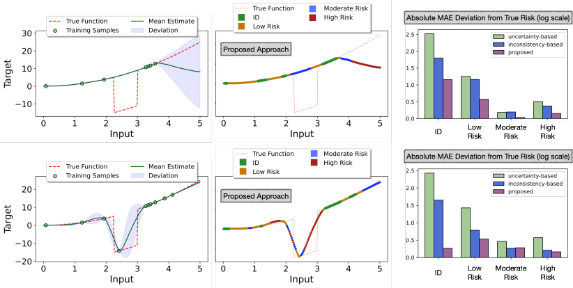
Figure 1: Epistemic uncertainty while necessary to estimate risk is not sufficient to completely characterize all risk regimes. Top: Out-of-support (OOS) samples in the range of $[2.2-2.7]$ exhibit low uncertainty but moderate model risk due to significant deviation from true function. Bottom: Even with better experiment designs, uncertainty alone in the extrapolating regime $[4.5-5]$ is unreliable due to potential drift from the truth. We propose PAGER, a framework that leverages anchoring [14] to unify prediction uncertainty and non-conformity to the training manifold. PAGER accurately flags those regimes as Moderate Risk (shown in blue) and outperforms existing baselines in accurately categorizing samples into appropriate data regimes consistent with the true risk (lower MAE).

2 Background and Related Work

Preliminaries. We consider a predictive model $F_{\theta}$, parameterized by $\theta$, trained on a labeled dataset $\mathcal{D}=\{(\mathrm{x}_{i},\mathrm{y}_{i})\}^{M}_{i=1}$ with $M$ samples. Note, each input $\mathrm{x}_{i}\in X$ and label $\mathrm{y}_{i}\in y$ belong to the spaces of inputs $X$ (in $d-$dimensions) and continuous-valued targets $y$ respectively. Given a non-negative loss function $\mathcal{L}$, e.g., absolute error $|\mathrm{y}-\mathrm{\hat{y}}|$, the sample-level risk of a predictor can be defined as $\mathrm{R}(\mathrm{x};F_{\theta})=\mathbb{E}_{y|\mathrm{x}}~{}{\mathcal{L}(\mathrm{y},F_{\theta}(\mathrm{x})})$. Basically, risk is defined as the cost incurred for incorrect predictions. While estimating true risk is challenging in practice due to the need for access to the unknown joint distribution $P(X,y)$, it becomes crucial to develop methods that can reliably flag and categorize different risk regimes to facilitate safe deployment of models. We now define the different regimes of generalization that we want to characterize: (i) In-distribution: This is the scenario where $P(\mathrm{x}_{t}\in X)>0$ and $P(\mathrm{x}_{t}\in\mathcal{D})>0$, i.e., there is likelihood for observing the test sample in the training dataset; (ii) Out-of-Support (OOS): The scenario where $P(\mathrm{x}_{t}\in X)>0$ but $P(\mathrm{x}_{t}\in\mathcal{D})=0$, i.e., the train and test sets have different supports, even though they are drawn from the same space; (iii) Out-of-Distribution (OOD): This is the scenario where $P(\mathrm{x}_{t}\in X)=0$, i.e., the input spaces for train and test data are disjoint. We illustrate the differences between OOS and OOD regimes in Figure 2 using 1D and 2D examples. In the 1D case, OOS corresponds to regimes where the likelihood of observing data in the training support is zero but is non-zero in the input-space. Data from regimes outside the input space are referred to as OOD. In the 2D case, OOS constitutes regimes with new combinations of features (light blue) which are not jointly but individually seen in the train data.

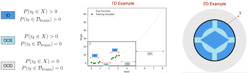
Figure 2: An illustration of different data regimes of generalization. Using examples in 1D and 2D, we show ID, OOS and OOD regimes.

Generalization Gap and Risk Prediction. Generalization error predictors estimate the difference in accuracy between an unlabeled, distribution shifted dataset with respect to a controlled validation data. Focused on classification, these methods estimate either sample level correctness scores (proxy for model risk) [16, 17] or distributional level metrics [1, 2, 18, 19, 20] to estimate the gap. Risk identification in regression problems is a relatively under-explored area of research. In that context, DEUP [12] has emerged as a leading approach that estimates predictive uncertainty as a surrogate for total loss using post-hoc error estimation. While DEUP has shown promising results, it is primarily centered around uncertainty; other methods such as DataSUITE [13] focus on identifying inconsistencies in the input space, while Data IQ [21] characterizes sub-groups in the data distribution using epoch-level statistics. These existing methods have limitations when it comes to accurately characterizing samples from all regimes on the test data. This motivates the need for the development of an effective risk identification method specifically designed for regression problems. A quick overview of the existing failure characterization methods in comparison to PAGER can be found in Appendix B.

Anchoring in Predictive Models. Anchoring is a principle employed in deep models which involves the reparameterization of an input sample $\mathrm{x}$ referred to as the query into a tuple comprising an anchor $\mathrm{r}$ drawn from the training distribution and the residual $\Delta\mathrm{x}$ denoted by $[\mathrm{r},\Delta\mathrm{x}]=[\mathrm{r},\mathrm{x}-\mathrm{r}]$ [14]. Anchoring thus induces a joint distribution that depends not only on $P(X)$, but also on the distribution of the residuals $P(\Delta)$. During training, anchoring ensures consistency in prediction for a query $\mathrm{x}$ by effectively modeling the combinatorial relationship between every sample in the dataset and infers the joint distribution $P(X,\Delta)$. During inference, we can obtain accurate predictions for a query $\mathrm{x}$ if $\mathrm{x}\in P(X)$ and $[\mathrm{x}-\mathrm{r}]\in P(\Delta)$. This idea has shown promising results in various tasks [14, 2, 22, 15] including uncertainty estimation, anomaly detection and extrapolation. Our framework PAGER makes an interesting finding that both uncertainty and non-conformity to the training manifold, two key components of failure characterization, can be estimated using the anchoring principle. We provide the detailed description of anchoring based methods in Appendix A of the supplementary material.

3 Characterizing and Detecting Failure in Deep Regressors

Generalization gap predictors in the classification setting aim to estimate the correctness of the predicted labels. However, defining failure becomes complex in regression tasks as the acceptable error tolerance can vary across different use cases. To address this, we first propose a novel framework for systematically characterizing failure in deep regression models. This framework organizes unlabeled samples from a test set into different regimes based on their levels of expected risk (low, moderate, high). By doing so, practitioners can gain a detailed understanding of a model’s generalization behavior. Next, we make a critical advancement to the challenging problem of estimating sample-level risk. Existing approaches utilize epistemic uncertainties or task-agnostic data inconsistency to define surrogate measures for expected risk. In contrast, our method leverages the principle of neural network anchoring [14, 15] to unify both prediction uncertainty and non-conformity to the training data manifold, which are subsequently used to derive the risk regimes. In addition to eliminating the need for separate estimators for uncertainties and the proposed scores, our approach does not require additional calibration data. Finally, we introduce a suite of evaluation metrics to quantitatively benchmark failure detectors in deep regression models.

3.1 A New Failure Characterization Framework

Since it is challenging to obtain accurate sample-level error estimates, particularly in regimes where models need to extrapolate – for e.g., in OOS or OOD cases – a more flexible solution is to analyze sample groups that correspond to varying levels of expected risk. Naturally, epistemic uncertainties provide a convenient way to identify sample deficiency. However, as illustrated in Figure 1, uncertainty estimates and true risk are not always correlated, thus making solely uncertainty-based failure detectors (e.g., DEUP [12]) to be ineffective in practice. This is partly because risk can arise from a variety of sources, only some of which are explained by epistemic uncertainty. While epistemic uncertainty can reflect failures corresponding to OOS or OOD test samples, larger errors can also arise when $(\mathrm{x}_{t},\mathrm{y}_{t})\notin P(X,y)$, i.e., regardless of the uncertainty on $\mathrm{x}_{t}$, the risk can be high when the test sample (and its unknown target) does not adhere to the data manifold. Consequently, it is essential to consider a complementary score that can quantify this discrepancy.

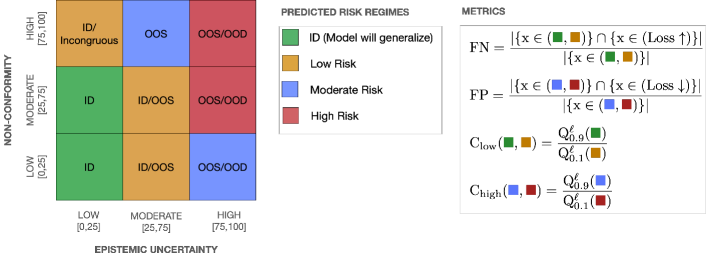
Figure 3: Overview of our proposed framework. PAGER organizes test examples into bins (low, moderate and high) using both predictive uncertainty and scores of non-conformity to the training manifold. With such a categorization, PAGER associates samples into $4$ levels of expected risk (ID, Low Risk, Moderate Risk and High Risk). We also develop a novel suite of metrics that enables a rigorous assessment of failure detectors and is more holistic than conventional metrics such as average error of top inconsistent samples.

We now describe our framework for deep regression models (Figure 3). At a high level, we organize the set of test samples based on both uncertainty and non-conformity. Both scores are then split into three bins using conditional quantile ranges (low:$[0,25]$, medium:$[25,75]$ and high:$[75,100]$), thereby creating a non-trivial partition of the test data into risk regimes. Without loss of generality, we assume that a typical test set contains samples close to the training distribution, as well as OOS and potential OOD samples. Note that even when this assumption does not hold and the test set does not contain distribution shifts, our proposed framework can still identify regimes with increasing levels of expected risk.

ID ($\blacksquare$): The model generalizes well in this regime and is expected to produce the lowest prediction error. In our framework, this corresponds to samples with low uncertainty and low/moderate non-conformity scores;

Low Risk ($\blacksquare$): Even when the uncertainty is low, the model can produce higher error than the ID samples, when there is incongruity (e.g., samples within a neighborhood having different target values). Similarly, for OOS samples with moderate uncertainties, the model can still extrapolate well and produce reduced risk. Hence, we define this regime as the collection of (low uncertainty, high non-conformity) and (moderate uncertainty, low/moderate non-conformity) samples;

Moderate Risk ($\blacksquare$): Since epistemic uncertainties can be inherently miscalibrated, OOS samples, which the model cannot extrapolate to, can be associated with moderate uncertainties. On the other hand, the model could reasonably generalize to OOD samples that are flagged with high uncertainties. Hence, we define this regime as the collection of (moderate uncertainty, high non-conformity) and (high uncertainty, low/moderate non-conformity) samples;

High Risk ($\blacksquare$): Finally, when both the uncertainty and non-conformity scores are high, there is no evidence that the model will behave predictably on those samples. In practice, this can correspond to both OOS and OOD samples.

3.2 Uncertainty and Non-conformity using Anchoring

The core element of our failure analysis framework revolves around the measurement of uncertainties, and non-conformity in situations where the ground truth label is unknown. While there are numerous options available for estimating epistemic uncertainty, measuring non-conformity has been recognized as a practical challenge. This is because most existing non-conformity scores require access to ground truth labels. In regression problems, existing methods for characterizing non-conformity include auto-encoding error-based scoring in DataSUITE [13] and feature conformal prediction [23]. The former employs an auto-encoder trained on a calibration dataset to measure the score, making it task-agnostic. However, the latter relies on ground truth labels from a calibration set and applies a conformal interval prediction approach to characterize test data, which is not applicable in our scenario. Notably, both approaches demonstrate compromised performance when the calibration dataset fails to adequately represent the expected shifts during testing. To overcome these challenges, we propose a unified approach based on anchored neural networks.

As introduced in Section 2, an anchored model is trained by transforming a training sample $\mathrm{x}$ into a tuple, $(\mathrm{r},\mathrm{x}-\mathrm{r})$ based on an anchor $\mathrm{r}$, which is also drawn randomly from the training dataset $\mathcal{D}$. Building upon the findings from [14], at test time, predictions from different anchor choices can be used to obtain the mean and uncertainty estimates as follows:

$$\mu(y_{t}|\mathrm{x}_{t})=\frac{1}{K}\sum_{k=1}^{K}F_{\theta^{*}}([\mathrm{r}_{k},\mathrm{x}_{t}-\mathrm{r}_{k}]);~{}~{}\sigma(y_{t}|\mathrm{x}_{t})=\sqrt{\frac{1}{K-1}\sum_{k=1}^{K}(F_{\theta^{*}}([\mathrm{r}_{k},\mathrm{x}_{t}-\mathrm{r}_{k}])-\mu)^{2}},$$ (1)

where $\mu$ and $\sigma$ are estimated by marginalizing across $K$ anchors $\{\mathrm{r}_{k}\}_{k=1}^{K}$ sampled from $\mathcal{D}$.

Non-conformity via reverse anchoring: Turning our attention to the assessment of non-conformity, we make a noteworthy observation regarding the flexibility of an anchored neural network. It is able to not only capture the relative representation of a query (i.e., test sample) in relation to an anchor (i.e., training sample), but also the reverse scenario. To elaborate, the prediction for an anchor sample $\mathrm{r}$ is given as $F([\mathrm{x}_{t},\mathrm{r}-\mathrm{x}_{t}])$, where $\mathrm{x}_{t}$ represents a test sample. Since the ground truth function value is known for the training samples, we can measure the non-conformity score for a query sample based on its ability to accurately recover the target of the anchor. Note, unlike existing approaches, this can be directly applied to unlabeled test samples and does not require explicit calibration.

Looking from another perspective, the original anchor-centric model ([14]) provides reliable predictions for an input $[\mathrm{r},\Delta]$ only when $\mathrm{r}\in\mathcal{D}$ and $\Delta\in P(\Delta)$. However, for OOD or OOS samples, if $\Delta\notin P(\Delta)$, the estimated uncertainty becomes large everywhere, and as a result becomes inherently unreliable in order to rank by levels of expected risk. In contrast, our proposed query-centric score overcomes this challenge by directly measuring the discrepancy with respect to the ground truth target. Specifically, we define our non-conformity score as follows:

$$\mathtt{Score_{1}}(\mathrm{x})=\max_{r\in\mathcal{D}}\bigg{\|}\mathrm{y}_{\mathrm{r}}-F([\mathrm{x},\mathrm{r}-\mathrm{x}])\bigg{\|}_{1}$$ (2)

It is important to note that we measure the largest discrepancy across the training dataset. In practice, this can be done for a small batch of randomly selected training samples (e.g., 100). As demonstrated in our results, our proposed non-conformity approach proves highly effective compared to state-of-the-art uncertainty-based and inconsistency-based failure detectors (refer to Figure 1).

Resolving medium and high risk regimes better:

A closer examination of Equation (2) reveals that for samples that are far away from the training manifold, the model prediction can be uniformly bad (i.e., extrapolation), as both $\mathrm{x}\notin\mathcal{D}$ and $\Delta\notin P(\Delta)$. This can make distinguishing between samples with moderate risk and those with high risk very challenging. To mitigate this situation, we propose an approach, which is similar in spirit to the bilinear transduction procedure in [15]. The key difference between the two approaches is that, since our formulation is query-centric, we need to make both the query $\mathrm{x}$ and $\Delta$ be in-distribution in order to enable the anchored model $F$ to reliably predict the target for the anchor. We achieve this using the following optimization problem:

$$\mathtt{Score_{2}}(\mathrm{x})=\max_{r\in\mathcal{D}}\bigg{\|}\mathrm{x}-\arg\min_{\bar{\mathrm{x}}}\bigg{(}\bigg{\|}\mathrm{y}_{\mathrm{r}}-F([\bar{\mathrm{x}},\mathrm{r}-\bar{\mathrm{x}}])\bigg{\|}_{1}+\lambda\mathcal{R}(\bar{\mathrm{x}})\bigg{)}\bigg{\|}_{2},$$

$$\text{where }\mathcal{R}(\bar{\mathrm{x}})=\bigg{\|}\bar{\mathrm{x}}-A([\mathrm{x},\bar{\mathrm{x}}-\mathrm{x}])\bigg{\|}_{2}+\bigg{\|}\mathrm{x}-A([\bar{\mathrm{x}},\mathrm{x}-\bar{\mathrm{x}}])\bigg{\|}_{2}.$$ (3)

In this approach, the score is measured as the discrepancy in the input space to a new fictitious sample that serves as an intermediate anchor, such that its prediction matches the known prediction on the training sample. In other words, we optimize the modification of the query sample $\mathrm{x}$ to $\bar{\mathrm{x}}$ in such a way that we accurately match the true target for the anchor $\mathrm{r}$. The non-conformity is then quantified as the amount of movement required in $\mathrm{x}$ to match the target. To ensure that the resulting $\bar{\mathrm{x}}$ remains within the input data manifold, we incorporate a regularizer $\mathcal{R}(\bar{\mathrm{x}})$. Specifically, we train an anchored auto-encoder $A$ on the training dataset $\mathcal{D}$ and enforce cyclical consistency, where $A$ is required to recover $\mathrm{x}$ using $\bar{\mathrm{x}}$ as the anchor and vice versa. While $\mathtt{Score_{1}}$ is extremely scalable, $\mathtt{Score_{2}}$ provides better resolution in the medium and high risk regimes at an increased compute cost. In general, the choice of the non-conformity score is determined by the constraints and risk tolerance in different applications. We provide the algorithm listings and details of all these models in Appendices C and D of the supplementary material respectively.

3.3 Evaluation Metrics

While the authors of [12] reported the Spearman correlation between the true risk and the predicted risk on a held-out test set, DataSUITE measured the average error in top inconsistent samples. Unfortunately, neither of these metrics comprehensively indicate the behavior of failure detectors in different risk regimes. Hence, we introduce a new suite of metrics (see Figure 3).

False Negatives (FN)($\downarrow$) This is the most important metric in applications, where the cost of missing to detect high risk failures is high. Hence, we measure the ratio of samples in the ID or Low Risk regimes that actually have high true risk (top $20^{\text{th}}$ percentile of all test samples).

False Negatives (FP)($\downarrow$) This reflects the penalty for scenarios where arbitrarily flagging harmless samples as failures. Here, we measure the ratio of samples in the Moderate or High Risk regimes that actually have low true risk (bottom $20^{\text{th}}$ percentile of all test samples).

Confusion in Low Risk Regimes (C${}_{\text{low}}$)($\downarrow$) A common challenge in fine-grained sample grouping (ID vs Low Risk) is that detection score can confuse samples between neighboring regimes. We define this metric to measure the ratio between the $90^{\text{th}}$ percentile of the ID regime and the $10^{\text{th}}$ percentile of the Low Risk regime.

Confusion in High Risk Regimes (C${}_{\text{high}}$)($\downarrow$) This is similar to the previous case and instead measures the confusion between the Moderate Risk and High Risk regimes.

4 Experiments

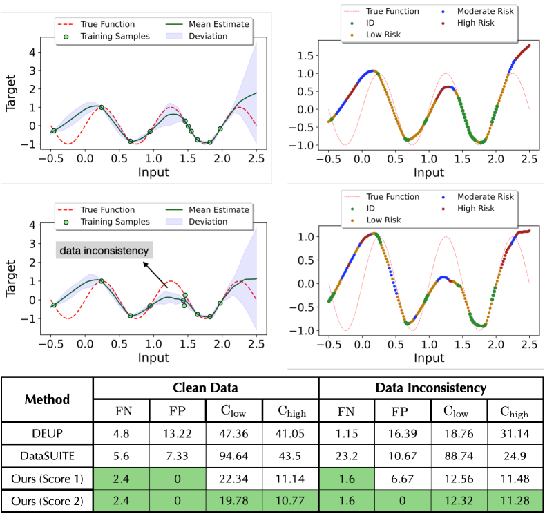
(a) Sinusoid

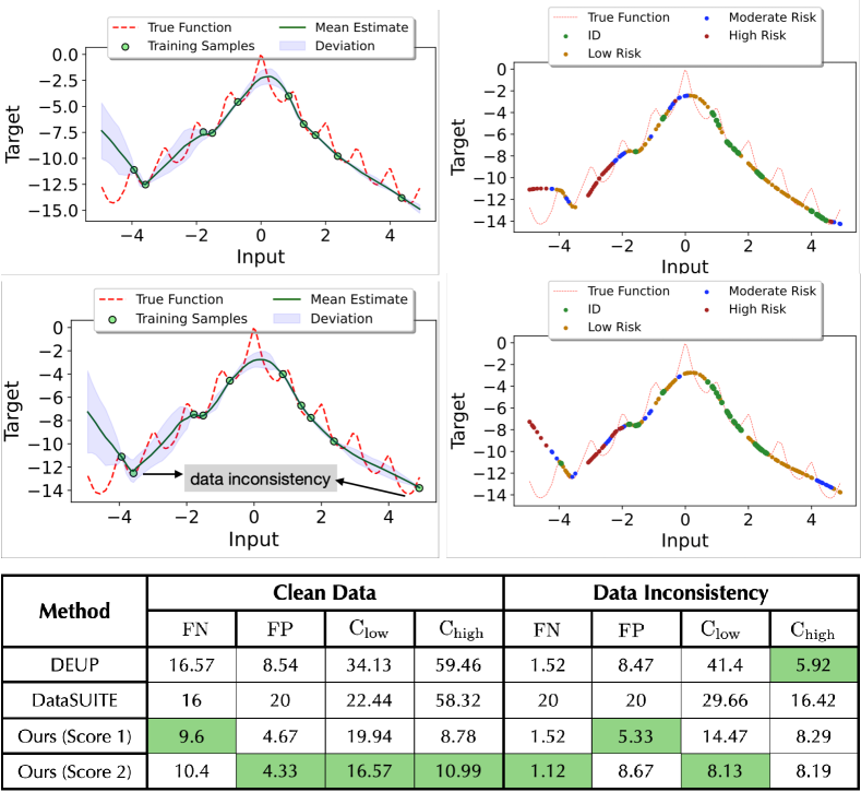
(b) Ackley1D

Figure 4: PAGER Effectively Characterizes Different Regimes of Model Failure. In both (a) and (b), we find that PAGER identifies the risk regimes reliably producing a well-calibrated transition as we traverse from the ID manifold to regimes of unobserved data. Importantly, PAGER produces significantly lower FN, FP and confusion metrics over the state-of-the-art baselines demonstrating its efficacy in deep regression.

Datasets. We evaluate our framework on various datasets to demonstrate its effectiveness in identifying risk regimes. The datasets used are as follows:

1. 1D Synthetic Functions: (a) Parabola: $Y=X^{2}$ with $X\in[0,5]$, introducing a constant shift in $Y$ between $[2.25,3]$; (b) Sinusoid: $Y=sin(X)$ with $X\in[-0.5,2.5]$; (c) Ackley function [24] with $X\in[-5,5]$. For each function, we create two variants of the training data: Clean (original samples) and Inconsistent (subset of samples are corrupted by additive noise $n\sim\mathcal{N}(0,0.05)$).

2. HD Regression Benchmarks: (a) Camel (2D), (b) Levy (2D) [24] characterized by multiple local and global minima, (c) Kinematics (8D), (d) Puma (8D) [25] which are simulated datasets of the forward dynamics of different robotic control arms, (e) Boston Housing (13D) [26] and (f) Ailerons (39D) [27] which is a dataset for predicting control action of the ailerons of an F16 aircraft. For each benchmark, we create two variants: Gaps (training exposed to data with targets between $(0-30^{th})$ and $(60-100^{th})$ percentiles) and Tails (training exposed to $(0-70^{th})$ percentiles of the targets) resulting in a total of 12 datasets.

3. Image Regression: (a) Chairs Tails, (b) Chairs Gaps, (c) Cell Count Tails and (d) Cell Count Gaps [28]. These datasets contain synthetic images of chairs and cells, with the task of predicting the number of cells and yaw angle, respectively. In case of the Tails benchmark, the training is exposed to images with number of cells $[50-150]$ and angles $[15-75]$ respectively and are evaluated on the entire target range and vice-versa for Gaps.

Baselines. (i) DEUP [12] is the state-of-the-art epistemic uncertainty estimator of deep models. It utilizes a post-hoc, auxiliary error predictor that learns to predict the risk of the underlying model which is considered as a surrogate for uncertainties; (ii) DataSUITE [13] is a task-agnostic approach that estimates the inconsistencies in the data regimes in order to assess data quality. Both the baselines however rely on the use of additional, curated calibration data to either train the error predictor in case of DEUP and to obtain non-conformity scores that assess the sample level quality in the latter.

Training Protocols. For all experiments reported in this paper, we adopt the open-source $\Delta-$UQ codebase (https://github.com/LLNL/DeltaUQ) [14]. With experiments on the tabular data, we use an MLP [29] with $4$ layers each with a hidden dimension of $128$. In case of image data, we employ a $40-2$ WideResNet architecture [30]. Without loss of generality, we utilize the $L_{1}$ objective for training the models. We provide the complete implementation details along with the hyper-parameters adopted in Appendix D of the supplement.

Ablations. We evaluated the failure detection performance using only (a) non-conformity score and (b) uncertainties arising from anchoring in order to understand the performance of using each of those components independently in lieu of jointly combining them as in PAGER. We report performance comparisons with PAGER on the tabular benchmarks in Appendix E (Table 1) of the supplement. We find that PAGER provides consistently superior results across all datasets.

Table 1: Assessing the identified risk regimes for HD Benchmarks (Gaps). We report the FN, FP, C${}_{\text{low}}$ and C${}_{\text{high}}$ metrics on evaluation data across the entire target regime (lower the better). Note that for every metric, we identify the first and second best approach across the different benchmarks.

Metrics	Method	Camel (2D)	Levy (2D)	Kinematics (8D)	Puma (8D)	Housing (13D)	Ailerons (39D)
	DEUP	15.79	9.25	17.6	13.2	11.46	14.4
	DataSUITE	21.74	19.69	18.4	16.8	17.71	11.2
	PAGER ($\mathtt{Score_{1}}$)	12.15	10.9	6.4	10.4	6.25	0.9
FN$\downarrow$	PAGER ($\mathtt{Score_{2}}$)	11.39	10.65	6.4	10.8	7.29	1.2
	DEUP	17.48	10.04	18.67	12.0	10.34	16.0
	DataSUITE	15.74	15.32	10.67	17.33	12.07	8.0
	PAGER ($\mathtt{Score_{1}}$)	3.36	5.04	12.0	9.67	8.62	4.0
FP$\downarrow$	PAGER ($\mathtt{Score_{2}}$)	7.56	4.2	10.67	8.83	9.07	1.33
	DEUP	50.59	34.67	10.71	14.82	13.86	15.55
	DataSUITE	42.92	71.06	21.96	15.26	14.8	30.78
	PAGER ($\mathtt{Score_{1}}$)	14.05	13.62	12.91	12.44	13.33	12.90
$\text{C}_{\text{low}}$$\downarrow$	PAGER ($\mathtt{Score_{2}}$)	10.13	10.41	10.93	8.71	10.42	11.18
	DEUP	15.47	12.42	11.28	6.18	3.36	23.94
	DataSUITE	37.51	36.5	5.97	10.57	22.56	4.2
	PAGER ($\mathtt{Score_{1}}$)	8.89	10.39	7.71	8.09	3.19	1.69
$\text{C}_{\text{high}}$$\downarrow$	PAGER ($\mathtt{Score_{2}}$)	11.03	9.37	7.01	7.30	2.95	1.65

Table 2: Assessing the identified risk regimes for HD Benchmarks (Tails). For every metric, we identify the first and second best approach across the different benchmarks.

Metrics	Method	Camel (2D)	Levy (2D)	Kinematics (8D)	Puma (8D)	Housing (13D)	Ailerons (39D)
	DEUP	10.53	7.34	14.4	16.8	2.11	18.4
	Data SUITE	3.84	9.21	17.6	22.4	17.89	17.6
	PAGER ($\mathtt{Score_{1}}$)	0.0	4.56	8	8.8	1.05	9.6
FN$\downarrow$	PAGER ($\mathtt{Score_{2}}$)	0.25	4.82	7.2	10.4	2.32	9.6
	DEUP	9.5	7.35	13.0	14.67	8.77	12.0
	Data SUITE	3.83	6.38	24.0	26.67	19.3	12.0
	PAGER ($\mathtt{Score_{1}}$)	0.42	1.68	6.33	13.33	3.51	0.8
FP$\downarrow$	PAGER ($\mathtt{Score_{2}}$)	1.68	2.52	6.18	12.2	4.26	0.4
	DEUP	34.04	52.74	6.36	5.37	13.0	11.07
	Data SUITE	42.08	81.06	7.34	5.67	17.73	16.52
	PAGER ($\mathtt{Score_{1}}$)	15.59	26.44	6.58	4.61	5.14	17.19
$\text{C}_{\text{low}}$$\downarrow$	PAGER ($\mathtt{Score_{2}}$)	14.37	14.04	5.73	5.5	6.67	11.38
	DEUP	23.69	20.75	6.83	2.63	5.69	7.25
	Data SUITE	17.49	27.32	10.08	6.41	5.15	4.97
	PAGER ($\mathtt{Score_{1}}$)	7.5	17.93	7.14	2.46	5.07	2.31
$\text{C}_{\text{high}}$$\downarrow$	PAGER ($\mathtt{Score_{2}}$)	6.7	15.18	7.09	2.81	4.05	2.43

5 Main Findings & Discussion

PAGER Systematically Identifies Failure Regimes in Deep Regression Models. To identify different risk regimes, it is crucial for a method to align well with the inferred data manifold (ID) and progressively flag regions of low, moderate and high risk as we move away from the training manifold. PAGER achieves this objective effectively, as illustrated in Figure 4. We observe that it accurately identifies the training data regimes (Green) as part of the ID. As we traverse further from the training manifold, PAGER  assigns low risk (Yellow) to unseen examples that are close to the training data. Notably, as we encounter samples that are significantly out-of-sample or out-of-distribution, we consistently identify them as Moderate or High risk. Importantly, PAGER ensures a well-calibrated transition between risk regimes across the entire input space. Our unified framework excels in characterizing regimes of moderate or low uncertainty, as demonstrated in Figure 4(a) where the regime $\mathtt{[-0.25,0]}$ appears to have moderate uncertainty but is correctly identified as moderate to high risk. Furthermore, PAGER provides reliable performance even in the presence of data inconsistencies. We include the detailed results for all the 1D benchmarks in Appendix F (Tables 2 and 3) of the supplement. Importantly, we also find PAGER to be significantly effective even on real-world tabular benchmarks characterized by complex distribution shifts, and include the comparison with baselines in Appendix F (Table 4) of the supplementary material.

Table 3: Comparison for runtime for different failure characterization approaches.

	Data Suite	DEUP	PAGER (Score 1)	PAGER (Score 2)
Runtime (sec) for 1000 samples with a single GPU	29.8	18.2	1.55	40.9

In addition to the fidelity metrics, computational efficiency is another important aspect of failure detectors in practice. Table 3 provides the inference run-times for the different methods measured using a test set of 1000 samples (1D benchmarks). DataSUITE involves training an autoencoder followed by conformalization, while DEUP requires an auxiliary risk estimator to evaluate risk. In comparison, computing $\mathtt{Score_{1}}$ with PAGER is very efficient as it basically involves only forward passes with the anchored model. $\mathtt{Score_{2}}$ on the other hand requires a test-time optimization guided by the manifold regularization objective. While $\mathtt{Score_{2}}$ comes with an increased computational cost, we find that it helps in resolving regimes of moderate and high risk better.

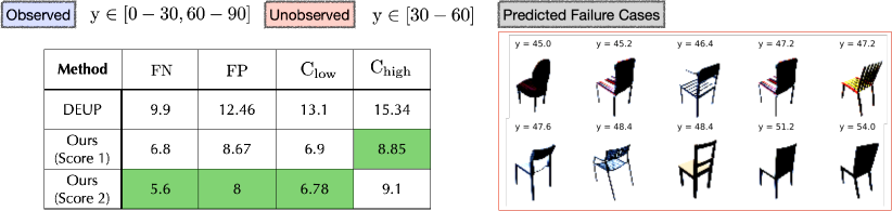
(a) Chair Angles (Gap)

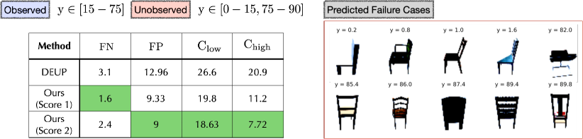
(b) Chair Angles (Tails)

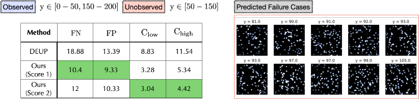
(c) Cells Count (Gap)

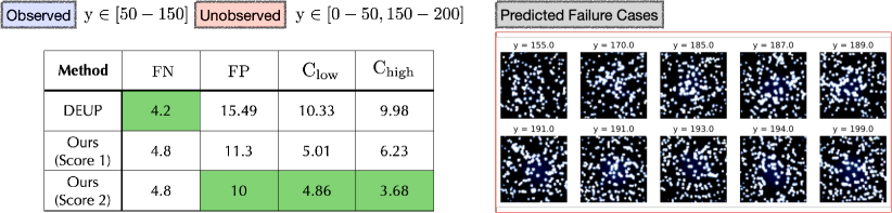
(d) Cells Count (Tails)

Figure 5: Efficacy of PAGER on Image Regression Benchmarks. We can observe that in comparison to the state-of-the art baseline DEUP, PAGER effectively minimizes the FN, FP and confusion metrics even under challenging extrapolation scenarios. We find that PAGER can consistently flag samples from the unobserved regimes which corresponds to highly erroneous predictions.

PAGER Produces Lower False Negatives and False Positives. As discussed in Section 3, it is vital to ensure that regimes that have been identified as ID or Low Risk do not correspond to large prediction errors and vice-versa thereby reducing FN and FP. It can be observed from Figure 4 that the use of PAGER to characterize failure significantly reduces the FN and FP in comparison to the state-of-the-art baselines. This highlights the limitations of relying solely on predictive uncertainties, such as DEUP, for failure characterization, as they can be insufficient in practical applications. Additionally, utilizing uncertainty methods such as DataSUITE that assess data quality without task-specific considerations may not accurately identify risk regimes. Remarkably, even in higher dimensions and more complex extrapolation scenarios (e.g., Gaps and Tails, as discussed in Section 4), PAGER consistently outperform the baselines. The results presented in Tables 1 and Table 2 demonstrate the effectiveness PAGER, showcasing an average reduction in FN and FP of $\approx 50\%$ and $\approx 56\%$, respectively on an average over the baselines.

PAGER Reduces Confusion Across the Failure Regimes. As described in Section 3, we can consider a score as completely reliable if it is able to effectively demarcate the risk regimes as per the true risk and reduce overlap as much as possible between them. It can be observed from Figure 4 and Tables 1 and Table 2 that our scores can significantly reduce the amount of overlap (C${}_{\text{low}}$ and C${}_{\text{high}}$) between the risk regimes making it reliable approach for identifying samples that can either generalize well or those that are completely OOD/OOS. The baselines on the other hand produce significantly higher confusion scores demonstrating their limitations in risk stratification.

$\mathtt{Score_{2}}~{}$Produces Non-Trivial Improvements Over $\mathtt{Score_{1}}$.  As described in Section 3, $\mathtt{Score_{2}}$ quantifies the non-conformities in the input space and requires a test-time optimization strategy to better enhance the identification of moderate and high risk regimes. Our findings across various benchmarks indicate that $\mathtt{Score_{2}}$ reduces FN and FP over $\mathtt{Score_{1}}$. Notably, $\mathtt{Score_{2}}$ exhibits a more conservative approach in characterizing risk regimes, resulting in comparatively lower confusion scores compared to $\mathtt{Score_{1}}$.

PAGER Reliably Characterizes Risk Even With Imaging Modalities. Our analysis in Figure 5 reveals that our framework achieves lower FN, FP, and confusion scores compared to the baseline methods, even when confronted with challenging extrapolation regimes in imaging datasets such as Chairs and Cells. This demonstrates the effectiveness of our approach in handling diverse modalities of data. Additionally, we provide sample images that were accurately identified as high risk by PAGER. Notably, these examples correspond to regimes that were not encountered during training. We further showcase the efficacy of PAGER on the task of CIFAR10 rotation angle prediction, where we considered a similar setting to Chair/Cells Gap in Appendix F (Table 5) of the supplement.

6 Broader Impact

In this paper, we propose PAGER, a framework for failure characterization in deep regression models. It leverages the principle of anchoring to integrate epistemic uncertainties and novel non-conformity scores, enabling the organization of samples into different risk regimes and facilitating a comprehensive analysis of model errors. We identify two key impacts. First, PAGER can enhance the safety of AI model deployment by proactively and preemptively detect failure cases in various high impact scenarios such as scientific simulations. This can prevent costly errors and mitigate risks associated with inaccurate predictions. Second, PAGER contributes to advancing research in failure characterization for deep regression. While we believe that it can improve reliability, its deployment and usage should be accompanied by ethical considerations and human oversight. Decisions and actions based on the detected failure cases should be made responsibly, taking into account potential biases, fairness, and broader societal impact.

APPENDIX

Appendix A Detailed Description of Anchoring in PAGER

PAGER expands on the recent successes in anchoring [14, 15] by building upon the $\Delta$-UQ methodology introduced in [14]. This methodology is used to estimate prediction uncertainties, which play a vital role in characterizing model risk regimes, as depicted in Figure 2 of the main paper. With that context, we now provide a concise overview of $\Delta-$UQ, its training and uncertainty estimation.

Overview: $\Delta-$UQ, short for $\Delta-$Uncertainty Quantification, is a highly efficient strategy for estimating predictive uncertainties that leverages anchoring. It belongs to the category of methods that estimate uncertainties using a single model [31, 32]. $\Delta-$UQ has been demonstrated to be an improved and scalable alternative to Deep Ensembles [8], eliminating the need to train multiple independent models for estimating uncertainties. The core idea behind $\Delta-$UQ is based on the observation that the injection of constant biases (anchors) to the input dataset produces different model predictions as a function of the bias. To that end, models trained using the same dataset but shifted by respective biases generates diverse predictions. This phenomenon arises from the fact that the neural tangent kernel (NTK)[33] induced in deep models lacks invariance to input data shifts [29]. Consequently, the variance among these models a.k.a anchored ensembles serves as a strong indicator of predictive uncertainty. Based on this observation, $\Delta-$UQ follows a simple strategy to consolidate the anchored ensembles into a single model training, where the input is reparameterized as an anchored tuple, as described in Section 2 of the main paper. It is important to note that $\Delta-$UQ performs anchoring in the input space for both vector-valued and image data.

Training: In this phase, for every training pair {$\mathrm{x},\mathrm{y}$} drawn from the dataset $\mathcal{D}$, a random anchor $\mathrm{r}_{k}$ is selected from the same training dataset. Both the input $\mathrm{x}$ and the anchor $\mathrm{r}_{k}$ are transformed into a tuple given as $[\mathrm{r}_{k},\mathrm{x}-\mathrm{r}_{k}]$. Importantly, this reparameterization does not alter the original predictive task, but instead of using only $\mathrm{x}$, the tuple $[\mathrm{r}_{k},\mathrm{x}-\mathrm{r}_{k}]$ is mapped to the target $\mathrm{y}$. For vector-valued data, $\Delta-$UQ constructs the tuples by concatenating the anchor $\mathrm{r}_{k}$ and the residual along the dimension axis. In the case of images, the tuples are created by appending along the channel axis, resulting in a $6-$channel tensor for each $3$-channel image. These tuples are organized into batches and used to train the models. Throughout the training process, in expectation, every sample $\mathrm{x}$ is anchored with every other sample in the dataset. The goal here is that the predictions for every $\mathrm{x}$ should remain consistent regardless of the chosen anchor. The training objective is given by:

$$\theta^{*}=\arg\underset{\theta}{\min}~{}~{}~{}\mathcal{L}(\mathrm{y},F_{\theta}([\mathrm{r}_{k},\mathrm{x}-\mathrm{r}_{k}]),$$ (4)

where $\mathcal{L}(.)$ is a loss function such as MAE or MSE. In effect, the $\Delta-$UQ training enforces that for every input sample $\mathrm{x}$, $F_{\theta}([\mathrm{r}_{1},\mathrm{x}-\mathrm{r}_{1}])=F_{\theta}([\mathrm{r}_{2},\mathrm{x}-\mathrm{r}_{2}])=\dots=F_{\theta}([\mathrm{r}_{k},\mathrm{x}-\mathrm{r}_{k}])$, where $F_{\theta}$ is the underlying model that operates on the tuple $([\mathrm{r}_{k},\mathrm{x}-\mathrm{r}_{k}])$ to predict $\mathrm{y}$.

Uncertainty Estimation: During the inference phase, using the trained model with weights $\theta^{*}$, we compute the prediction $\mathrm{y_{t}}$ for any test sample $\mathrm{x_{t}}$. This is performed by averaging the predictions across $K$ randomly selected anchors drawn from the training dataset. The standard deviation of these predictions is then used as the estimate for predictive uncertainty. The equations for calculating the mean prediction and uncertainty around a sample can be found in Equation 1 of the main paper.

Appendix B Comparison to Existing Failure Characterization Approaches

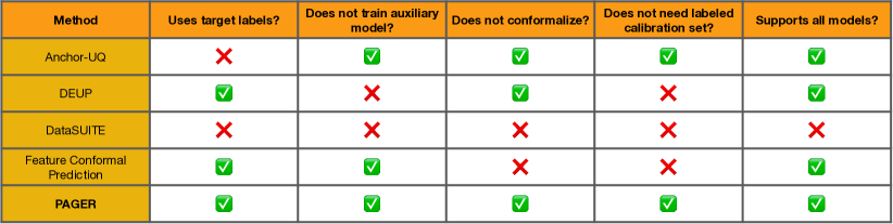
Figure 6: Comparison of PAGER to existing approaches for failure characterization in regression models.

To better clarify the differences between PAGER and existing approaches for failure characterization, we provide a high-level comparison in Figure 6. Notably, we conceptually study PAGER in comparison to existing epistemic uncertainty-based and conformal prediction-based alternatives. On one hand, as we argued in the main paper, epistemic uncertainties, despite their flexible, are insufficient to characterize all regimes of risk. On the other hand, the goal of conformal prediction (CP) approaches is to transform a non-conformity (NC) metric (e.g., absolute error) into prediction intervals with guaranteed coverage [34, 35]. While these intervals are well calibrated, it is not customary to assess their utility in ranking samples based on risk (low, moderate or high). Though it is possible to compute thresholds for different regimes with CP, they will be effective only when the ranking of samples is accurately preserved (much stronger guarantee than finite sample coverage). For e.g., DataSUITE relies on CP and our results show that it is effective only at detecting very high risk samples (OOD). Instead, for the first time, we find that a combination of epistemic uncertainty along with the proposed NC scores strongly correlate with risk in all regimes. Note, PAGER does not transform the non-conformity into intervals, and in fact, estimates the score even for test data unlike CP. Finally, PAGER provides a fundamentally new perspective into anchoring and shows how NC can be estimated with even unlabeled data (calibration or test).

Appendix C Algorithm Listings for PAGER

Algorithms 1,2 and 3 provide the details for estimating predictive uncertainty, non-conformity scores - $\mathtt{Score_{1}}$ and $\mathtt{Score_{2}}~{}$ respectively in PAGER.

Algorithm 1 PAGER: Predictive Uncertainty Estimation

1:  Input:  Input test samples $\{\mathrm{x}^{t}_{i}\}_{i=1}^{N}$, Pre-trained anchored model $F_{\theta^{*}}$,  Anchors $\{\mathrm{r}_{k}\}_{k=1}^{K}$ drawn from the training dataset $\mathcal{D}$

2:  Output:  Predictive Uncertainties ($\mathtt{Unc}$) for $\{\mathrm{x}^{t}_{i}\}_{i=1}^{N}$

3:  Initialize: $\mathtt{Unc}=\mathtt{list}()$

4:  for $i$ in $1$ to $N$ do

5:     $\mu(y^{t}_{i}|\mathrm{x}^{t}_{i})=\frac{1}{K}\sum_{k=1}^{K}F_{\theta^{*}}([\mathrm{r}_{k},\mathrm{x}^{t}_{i}-\mathrm{r}_{k}])$;

6:     $\sigma(y^{t}_{i}|\mathrm{x}^{t}_{i})=\sqrt{\frac{1}{K-1}\sum_{k=1}^{K}(F_{\theta^{*}}([\mathrm{r}_{k},\mathrm{x}^{t}_{i}-\mathrm{r}_{k}])-\mu(y^{t}_{i}|\mathrm{x}^{t}_{i}))^{2}}$;

7:     $\mathtt{Unc[i]}=\sigma(y^{t}_{i}|\mathrm{x}^{t}_{i})$

8:  end for

9:  return: $\mathtt{Unc}$

Algorithm 2 PAGER: $\mathtt{Score_{1}}$ Computation

1:  Input:  Input test samples $\{\mathrm{x}^{t}_{i}\}_{i=1}^{N}$, Pre-trained anchored model $F_{\theta^{*}}$,  Train data subset $\{\mathrm{r}_{k},\mathrm{y}_{k}\}_{k=1}^{K}$

2:  Output:  $\mathtt{Score_{1}}$ for $\{\mathrm{x}^{t}_{i}\}_{i=1}^{N}$

3:  Initialize: $\mathtt{Score_{1}}=\mathtt{list}()$

4:  for $i$ in $1$ to $N$ do

5:     $\mathtt{s}=\underset{k}{\max}\bigg{\|}\mathrm{y}_{k}-F_{\theta^{*}}([\mathrm{x}^{t}_{i},\mathrm{r}_{k}-\mathrm{x}^{t}_{i}])\bigg{\|}_{1}~{}~{}\forall k\in\{1\cdots K\}$;

6:     $\mathtt{Score_{1}[i]}=\mathtt{s}$

7:  end for

8:  return: $\mathtt{Score_{1}}$

Algorithm 3 PAGER: $\mathtt{Score_{2}}$ Computation

1:  Input:  Input test samples $\{\mathrm{x}^{t}_{i}\}_{i=1}^{N}$, Pre-trained anchored model $F_{\theta^{*}}$, Pre-trained anchored auto-encoder $A$,  Train data subset $\{\mathrm{r}_{k},\mathrm{y}_{k}\}_{k=1}^{K}$, Learning rate $\eta$, Weighing Factor $\lambda$, No. of iterations $T$

2:  Output:  $\mathtt{Score_{2}}$ for $\{\mathrm{x}^{t}_{i}\}_{i=1}^{N}$

3:  Initialize: $\mathtt{Score_{2}}=\mathtt{list()}$

4:  for $i$ in $1$ to $N$ do

5:     Initialize: $\bar{\mathrm{x}}\leftarrow\mathrm{x}^{t}_{i}$

6:     for $iter$ in $1$ to $T$ do

7:        Compute $\mathcal{R}(\bar{\mathrm{x}})=\bigg{\|}\bar{\mathrm{x}}-A([\mathrm{x}^{t}_{i},\bar{\mathrm{x}}-\mathrm{x}^{t}_{i}])\bigg{\|}_{2}+\bigg{\|}\mathrm{x}^{t}_{i}-A([\bar{\mathrm{x}},\mathrm{x}^{t}_{i}-\bar{\mathrm{x}}])\bigg{\|}_{2}.$

8:        Compute $L=\frac{1}{K}\underset{k}{\sum}\|\mathrm{y}_{k}-F_{\theta^{*}}([\bar{\mathrm{x}},\mathrm{r}_{k}-\bar{\mathrm{x}}])\|_{1}+\lambda\mathcal{R}(\bar{\mathrm{x}})$

9:        Update $\bar{\mathrm{x}}\leftarrow\bar{\mathrm{x}}-\eta\nabla_{\bar{\mathrm{x}}}L$

10:     end for

11:     $\mathtt{Score_{2}[i]}=\|\mathrm{x}-\bar{\mathrm{x}}\|_{2}$

12:  end for

13:  return: $\mathtt{Score_{2}}$

Appendix D Description of our Training Protocols

D.1 Datasets

(a) 1D regression benchmarks. For evaluating the behavior of PAGER in 1D benchmarks, we used the following standard black-box functions:

1. $f_{1}(\mathrm{x})$ = $\begin{cases*}\phantom{-}\mathrm{x}^{2}&if $\mathrm{x}<2.25\phantom{x}\text{or}\phantom{x}\mathrm{x}>3.01$\\ \phantom{-}\mathrm{x}^{2}-20&otherwise\end{cases*}$ (Figure 1 in the main paper)

2. $f_{2}(\mathrm{x})=\sin(2\pi\mathrm{x})$, $\mathrm{x}\in[-0.5,2.5]$ (Figure 3a in the main paper)

3. $f_{3}(\mathrm{x})=a\exp(-b\mathrm{x})+\exp(\cos(c\mathrm{x}))-a-\exp(1)$, $\mathrm{x}\in[-5,5]$, $a=20,b=0.2,c=2\pi$ (Figure 3b in the main paper)

4. $f_{4}(\mathrm{x})=\sin(\mathrm{x})\cos(5\mathrm{x})\cos(22\mathrm{x})$, $\mathrm{x}\in[-1,2]$

In each of these functions, we used $200$ test samples drawn from an uniform grid and computed the evaluation metrics.

(b) HD regression benchmarks. For this experiment, we used standard regression functions in varying dimensions ($2$D to $39$D) and different sample sizes (Camel, Levy: $100$ samples for training and $400$ samples for testing; for the HD benchmarks we used $2500$ samples for training and $400$ samples for testing).

Table 4: Ablation. We present comparisons to two baselines that independently consider the non-conformity and anchoring-based uncertainty scores for failure characterization. Our results clear evidence the importance of considering both scores jointly.

Metrics	Method	$f_{1}(\mathrm{x})$	$f_{2}(\mathrm{x})$	$f_{3}(\mathrm{x})$	$f_{4}(\mathrm{x})$
	NC-only	6.19	2.2	13.7	8.8
	Anchor-UQ	5.95	5.37	14.5	11.8
	DEUP	6.19	6.56	16.57	27.13
FP$\downarrow$	PAGER ($\mathtt{Score_{1}}$)	5.6	0	11.6	2.4
	NC-only	9.93	10.42	8.81	12.18
	Anchor-UQ	5.05	4.9	6.54	6.01
	DEUP	8.91	3.41	8.54	9.09
FN$\downarrow$	PAGER ($\mathtt{Score_{1}}$)	1.33	2.67	4.33	4
	NC-only	57.54	40.1	31.66	52.24
	Anchor-UQ	40.7	19.88	25.59	98.92
	DEUP	65.9	57.86	34.13	169.54
$\text{C}_{\text{low}}\downarrow$	PAGER ($\mathtt{Score_{1}}$)	28.08	7.19	19.94	12.05
	NC-only	33.09	18.85	29.98	20.31
	Anchor-UQ	36.05	7.75	17.9	11.56
	DEUP	91.64	4.47	59.46	16.56
$\text{C}_{\text{high}}\downarrow$	PAGER ($\mathtt{Score_{1}}$)	3.09	3.43	8.78	6.9

(c) Image regression benchmarks. Chair Angles (Gap/Tail) and Cells Count (Gap/Tail) [28] datasets contain RGB images each of dimensions $3\times 64\times 64$. For our experiments, we selected a subset of $5000$ examples from each dataset to train the anchored models, which were then used by PAGER for uncertainty estimation and score computation. For evaluation, we used a random subset of $400$ examples from both seen and unseen data regimes encountered while training.

D.2 Hyper-parameters

In the case of image regression benchmarks, we train an anchored $40-2$ WideResnet model. The training is performed with a batch size of $128$ for $100$ epochs. We utilize the ADAM optimizer with momentum parameters of $(0.9,0.999)$ and a fixed learning rate of $1e-4$. To train the anchored auto-encoder for computing $\mathtt{Score_{2}}$, we employ a convolutional architecture with an encoder-decoder structure. The encoder consists of two convolutional layers with kernel sizes of $(3,3)$ and appropriate padding, as well as MaxPooling operations. The decoder comprises two transposed convolutional layers with stride $2$ to reconstruct the input images. We train the anchored auto-encoder using a batch size of $128$ for $100$ epochs. The ADAM optimizer with momentum parameters $(0.9,0.999)$, and a fixed learning rate of $1e-3$, is used for training. For the other regression benchmarks, we used a standard MLP with $5$ hidden layers, ReLU activation and batchnorm. They were all trained for $5000$ epochs with learning rate $5e-5$ and ADAM optimizer.

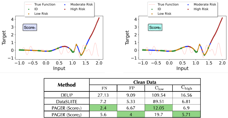
Figure 7: PAGER results for the 1D benchmark function $f_{4}(\mathrm{x})$. Similar to the previous examples showed in the main paper, PAGER is consistently superior to DEUP and DataSUITE baselines.

Appendix E Ablations

While PAGER jointly considers both anchoring-based uncertainties and non-conformity scores to identify different risk regimes, it is important understand the performance of using each of those components independently. To this end, we create the two following baselines and report performance comparisons on the tabular benchmarks.

NC-only. Our NC scores (Scores 1 and 2) measure either the relative change in the target value or distances in the input space. Since those scores are unnormalized, they behave differently across different data regimes. For e.g., NC scores can be high for scenarios where epistemic uncertainties are high or low (Fig. 1 in the main paper). Hence, they are insufficient to accurately rank samples on their own. However, designing a normalization strategy that works even for unseen test data is non-trivial, and hence PAGER works with unnormalized scores only. Table 4 shows results for the 1D benchmarks used in our study. While NC-only baseline can reasonably control FP, it is not able to reduce the FN.

Anchor-UQ. In this baseline, we directly utilized the uncertainties from $\Delta$-UQ to detect risk regimes. Table 4 includes the performance assessment for this baseline as well. We observe that uncertainties from the anchored model are a much more effective baseline, even outperforming DEUP in all cases.

In comparison to both these baselines, PAGER leads to significant improvements in all metrics, emphasizing the importance of considering both uncertainty and non-conformity together.

Table 5: Metrics for 1D Benchmarks. We report the FN, FP, C${}_{\text{low}}$ and C${}_{\text{high}}$ metrics on evaluation data across the entire target regime (lower the better). Note that for every metric, we identify the first and second best approach across the different benchmarks.

Metrics	Method	$f_{1}(\mathrm{x})$	$f_{2}(\mathrm{x})$	$f_{3}(\mathrm{x})$	$f_{4}(\mathrm{x})$
	DEUP	6.19	6.56	16.57	27.13
	DataSUITE	14	8.8	16	7.2
	PAGER ($\mathtt{Score_{1}}$)	5.6	0	11.6	2.4
FN$\downarrow$	PAGER ($\mathtt{Score_{2}}$)	4.8	5.6	8.4	5.6
	DEUP	8.91	3.41	8.54	9.09
	DataSUITE	18.67	16	20	5.33
	PAGER ($\mathtt{Score_{1}}$)	2.67	0	4.67	6.67
FP$\downarrow$	PAGER ($\mathtt{Score_{2}}$)	1.33	2.67	4.33	4
	DEUP	65.9	57.86	34.13	169.54
	DataSUITE	59.42	24.61	22.44	89.51
	PAGER ($\mathtt{Score_{1}}$)	28.08	7.19	19.94	12.05
$\text{C}_{\text{low}}$$\downarrow$	PAGER ($\mathtt{Score_{2}}$)	20.61	17.8	16.57	19.7
	DEUP	91.64	4.47	59.46	16.56
	DataSUITE	3.66	46.02	58.32	6.81
	PAGER ($\mathtt{Score_{1}}$)	3.09	3.43	8.78	6.9
$\text{C}_{\text{high}}$$\downarrow$	PAGER ($\mathtt{Score_{2}}$)	3.09	4.67	10.99	5.71

Table 6: Metrics for 1D benchmark functions, when input data inconsistencies are synthetically introduced. We report the FN, FP, C${}_{\text{low}}$ and C${}_{\text{high}}$ metrics on evaluation data across the entire target regime (lower the better). Note that for every metric, we identify the first and second best approach across the different benchmarks.

Metrics	Method	$f_{1}(\mathrm{x})$	$f_{2}(\mathrm{x})$	$f_{3}(\mathrm{x})$	$f_{4}(\mathrm{x})$
	DEUP	9.3	9.97	1.15	1.52
	DataSUITE	21.6	2.8	23.2	20
	PAGER ($\mathtt{Score_{1}}$)	4.8	4.8	1.6	1.52
FN$\downarrow$	PAGER ($\mathtt{Score_{2}}$)	4.8	8	1.6	1.12
	DEUP	6.12	10.83	16.39	8.47
	DataSUITE	16	4.33	10.67	20
	PAGER ($\mathtt{Score_{1}}$)	5.33	2.67	6.67	5.33
FP$\downarrow$	PAGER ($\mathtt{Score_{2}}$)	5.33	2.67	3.93	8.67
	DEUP	17.63	61.86	18.76	41.4
	DataSUITE	37.14	24.24	88.74	29.66
	PAGER ($\mathtt{Score_{1}}$)	13.49	11.7	12.56	14.47
$\text{C}_{\text{low}}$$\downarrow$	PAGER ($\mathtt{Score_{2}}$)	15.24	16.77	12.32	8.13
	DEUP	14.4	14.22	31.14	5.92
	DataSUITE	10.56	11.42	24.9	16.42
	PAGER ($\mathtt{Score_{1}}$)	11.47	12.35	11.48	8.29
$\text{C}_{\text{high}}$$\downarrow$	PAGER ($\mathtt{Score_{2}}$)	6.89	8.45	11.28	8.19

Appendix F Additional Results

Table 7: Additional results with synthetic and real-world distribution shifts. While we used synthetic shifts (Gaps) for Airfoil and NO2, real-world shifts were used in the cases of SkillCraft and DTI. For every metric, we identify the first and second best approach across the different benchmarks. Corroborating with our findings in the paper, PAGER consistently outperforms existing baselines across all four metrics.

Metrics	Method	Airfoil	NO2	SkillCraft	DTI
	DEUP	8.81	2.27	7.83	16.51
	Data SUITE	5.95	6.58	13.45	29.18
	PAGER ($\mathtt{Score_{1}}$)	0.75	0	4.43	9.26
FN$\downarrow$	PAGER ($\mathtt{Score_{2}}$)	1.04	0.9	6.6	10.11
	DEUP	6.24	11.79	14.33	19.7
	Data SUITE	6.35	18.33	17.03	30.93
	PAGER ($\mathtt{Score_{1}}$)	3.56	4.18	8.91	9.94
FP$\downarrow$	PAGER ($\mathtt{Score_{2}}$)	3.82	3.05	10.5	10.29
	DEUP	28.23	19.32	5.47	5.5
	Data SUITE	37.11	47.6	6.92	12.8
	PAGER ($\mathtt{Score_{1}}$)	11.8	7.01	4.72	2.56
$\text{C}_{\text{low}}$$\downarrow$	PAGER ($\mathtt{Score_{2}}$)	9.93	6.15	5.8	2.83
	DEUP	17.99	7.71	6.69	10.05
	Data SUITE	14.85	6.82	7.01	18.93
	PAGER ($\mathtt{Score_{1}}$)	4.72	4.12	2.94	5.22
$\text{C}_{\text{high}}$$\downarrow$	PAGER ($\mathtt{Score_{2}}$)	3.9	2.83	2.05	4.19

Table 8: Additional results CIFAR-10 rotation angle prediction. With a ResNet-34 backbone, we consider the task of predicting the rotation angle of an image from the CIFAR-10 dataset. For every metric, we identify the first and second best approach across the different benchmarks.

Metrics	Method	CIFAR-10
	DEUP	14.9
	Anchor-UQ	11.7
FP$\downarrow$	PAGER ($\mathtt{Score_{1}}$)	3.3
	DEUP	15.2
	Anchor-UQ	13.7
FN$\downarrow$	PAGER ($\mathtt{Score_{1}}$)	7.8
	DEUP	18.8
	Anchor-UQ	19.6
$\text{C}_{\text{low}}$$\downarrow$	PAGER ($\mathtt{Score_{1}}$)	11.1
	DEUP	27.5
	Anchor-UQ	25.8
$\text{C}_{\text{high}}$$\downarrow$	PAGER ($\mathtt{Score_{1}}$)	11.3

1D Benchmarks: In addition to the $1$D regression results shown in the main paper, we now provide additional results for the benchmark function $f_{4}(\mathrm{x})$ in Figure 7. Furthermore, we provide comparisons of the four proposed metrics (FP, FN, $\text{C}_{\text{low}}$, $\text{C}_{\text{high}}$) in Table 5. We note that, PAGER consistently produces improvements to all metrics, when compared to existing uncertainty-based and inconsistency-based failure detectors.

In addition to the vanilla setting, we also emulated the scenario of data inconsistency (where $25\%$ randomly chosen training sample inputs were perturbed with additive Gaussian noise) and evaluated the performance metrics for all benchmark functions. Table 6 illustrates the performance of baselines and the two variants of PAGER. While PAGER performs the best among the compared methods, in this case, the regularized variant $\mathtt{Score_{2}}$ behaves more reliably.

Real-world Regression Datasets: In addition to the tabular datasets presented in the main paper, we also evaluate PAGER on $4$ more regression benchmarks, namely Airfoil, NO2, Skillcraft and Drug-Target Interactions (DTI). The details on these datasets can be found in [36]. While we used synthetic shifts (Gaps) for Airfoil and NO2 datasets, similar to the experiments in the main paper, real-world shifts were used in the cases of SkillCraft and DTI. More specifically, different league indices were used to emulate source and target distributions for Skillcraft, where different periods of observation were used for failure characterization in the DTI benchmark. Table 7 illustrates the results for these datasets and we find that PAGER significantly outperforms the baselines on all the four metrics even in this expanded evaluation.

CIFAR-10 Rotation Angle Prediction: For this task, we randomly applied a rotation transformation [0 - 90 degrees] to each 32x32x3 image and trained a ResNet-34 model to predict the angle of rotation. Following our other imaging experiments, we used the GAPS setting – rotation angles [0 - 45 degrees] and [70 - 90 degrees] were used to train, while the test data can have images that are rotated by any angle from [0 - 90 degrees]. Note, our evaluation is carried out using the 10K held-out test set (randomly rotated). Here, we report the failure detection performance (same evaluation protocol as the ones reported in the main paper). We show the results for the DEUP baseline, Anchor-UQ (a new baseline based on only uncertainties from anchoring) and PAGER ($\mathtt{Score_{1}}$). This strongly corroborates with our findings in the other experiments, and  ($\mathtt{Score_{1}}$) consistently outperforms the baselines.

References

- Guillory et al. [2021] Devin Guillory, Vaishaal Shankar, Sayna Ebrahimi, Trevor Darrell, and Ludwig Schmidt. Predicting with confidence on unseen distributions. In Proceedings of the IEEE/CVF International Conference on Computer Vision, pages 1134–1144, 2021.
- Narayanaswamy et al. [2022] Vivek Narayanaswamy, Rushil Anirudh, Irene Kim, Yamen Mubarka, Andreas Spanias, and Jayaraman J Thiagarajan. Predicting the generalization gap in deep models using anchoring. In ICASSP 2022-2022 IEEE International Conference on Acoustics, Speech and Signal Processing (ICASSP), pages 4393–4397. IEEE, 2022.
- Baek et al. [2022] Christina Baek, Yiding Jiang, Aditi Raghunathan, and J Zico Kolter. Agreement-on-the-line: Predicting the performance of neural networks under distribution shift. Advances in Neural Information Processing Systems, 35:19274–19289, 2022.
- Luo et al. [2022] Renqian Luo, Liai Sun, Yingce Xia, Tao Qin, Sheng Zhang, Hoifung Poon, and Tie-Yan Liu. Biogpt: generative pre-trained transformer for biomedical text generation and mining. Briefings in Bioinformatics, 23(6), 2022.
- Young et al. [2020] Albert T Young, Mulin Xiong, Jacob Pfau, Michael J Keiser, and Maria L Wei. Artificial intelligence in dermatology: a primer. Journal of Investigative Dermatology, 140(8):1504–1512, 2020.
- Huang and Chen [2020] Yu Huang and Yue Chen. Autonomous driving with deep learning: A survey of state-of-art technologies. arXiv preprint arXiv:2006.06091, 2020.
- Raissi et al. [2019] Maziar Raissi, Paris Perdikaris, and George E Karniadakis. Physics-informed neural networks: A deep learning framework for solving forward and inverse problems involving nonlinear partial differential equations. Journal of Computational physics, 378:686–707, 2019.
- Lakshminarayanan et al. [2017] Balaji Lakshminarayanan, Alexander Pritzel, and Charles Blundell. Simple and scalable predictive uncertainty estimation using deep ensembles. Advances in neural information processing systems, 30, 2017.
- Gal and Ghahramani [2016] Yarin Gal and Zoubin Ghahramani. Dropout as a bayesian approximation: Representing model uncertainty in deep learning. In international conference on machine learning, pages 1050–1059. PMLR, 2016.
- He et al. [2020] Bobby He, Balaji Lakshminarayanan, and Yee Whye Teh. Bayesian deep ensembles via the neural tangent kernel. Advances in Neural Information Processing Systems, 33:1010–1022, 2020.
- Amini et al. [2020] Alexander Amini, Wilko Schwarting, Ava Soleimany, and Daniela Rus. Deep evidential regression. Advances in Neural Information Processing Systems, 33:14927–14937, 2020.
- Lahlou et al. [2023] Salem Lahlou, Moksh Jain, Hadi Nekoei, Victor I Butoi, Paul Bertin, Jarrid Rector-Brooks, Maksym Korablyov, and Yoshua Bengio. DEUP: Direct epistemic uncertainty prediction. Transactions on Machine Learning Research, 2023. ISSN 2835-8856. URL https://openreview.net/forum?id=eGLdVRvvfQ.
- Seedat et al. [2022a] Nabeel Seedat, Jonathan Crabbé, and Mihaela van der Schaar. Data-SUITE: Data-centric identification of in-distribution incongruous examples. In Proceedings of the 39th International Conference on Machine Learning, volume 162, pages 19467–19496, 17–23 Jul 2022a. URL https://proceedings.mlr.press/v162/seedat22a.html.
- Thiagarajan et al. [2022] Jayaraman J. Thiagarajan, Rushil Anirudh, Vivek Narayanaswamy, and Peer timo Bremer. Single model uncertainty estimation via stochastic data centering. In Alice H. Oh, Alekh Agarwal, Danielle Belgrave, and Kyunghyun Cho, editors, Advances in Neural Information Processing Systems, 2022. URL https://openreview.net/forum?id=j0J9upqN5va.
- Netanyahu et al. [2023] Aviv Netanyahu, Abhishek Gupta, Max Simchowitz, Kaiqing Zhang, and Pulkit Agrawal. Learning to extrapolate: A transductive approach. In The Eleventh International Conference on Learning Representations, 2023. URL https://openreview.net/forum?id=lid14UkLPd4.
- Ng et al. [2022] Nathan Ng, Kyunghyun Cho, Neha Hulkund, and Marzyeh Ghassemi. Predicting out-of-domain generalization with local manifold smoothness. arXiv preprint arXiv:2207.02093, 2022.
- Jiang et al. [2022] Yiding Jiang, Vaishnavh Nagarajan, Christina Baek, and J Zico Kolter. Assessing generalization of SGD via disagreement. In International Conference on Learning Representations, 2022. URL https://openreview.net/forum?id=WvOGCEAQhxl.
- Chen et al. [2021] Mayee Chen, Karan Goel, Nimit S Sohoni, Fait Poms, Kayvon Fatahalian, and Christopher Ré. Mandoline: Model evaluation under distribution shift. In International Conference on Machine Learning, pages 1617–1629. PMLR, 2021.
- Jiang et al. [2019] Yiding Jiang, Dilip Krishnan, Hossein Mobahi, and Samy Bengio. Predicting the generalization gap in deep networks with margin distributions. In International Conference on Learning Representations, 2019. URL https://openreview.net/forum?id=HJlQfnCqKX.
- Deng and Zheng [2021] Weijian Deng and Liang Zheng. Are labels always necessary for classifier accuracy evaluation? In Proceedings of the IEEE/CVF Conference on Computer Vision and Pattern Recognition, pages 15069–15078, 2021.
- Seedat et al. [2022b] Nabeel Seedat, Jonathan Crabbé, Ioana Bica, and Mihaela van der Schaar. Data-IQ: Characterizing subgroups with heterogeneous outcomes in tabular data. In Alice H. Oh, Alekh Agarwal, Danielle Belgrave, and Kyunghyun Cho, editors, Advances in Neural Information Processing Systems, 2022b. URL https://openreview.net/forum?id=qC2BwvfaNdd.
- Trivedi et al. [2023] Puja Trivedi, Mark Heimann, Rushil Anirudh, Danai Koutra, and Jayaraman J. Thiagarajan. Estimating epistemic uncertainty of graph neural networks. In Data Centric Machine Learning Workshop @ ICML, 2023.
- Teng et al. [2023] Jiaye Teng, Chuan Wen, Dinghuai Zhang, Yoshua Bengio, Yang Gao, and Yang Yuan. Predictive inference with feature conformal prediction. In The Eleventh International Conference on Learning Representations, 2023. URL https://openreview.net/forum?id=0uRm1YmFTu.
- [24] Virtual library of simulation experiments. https://www.sfu.ca/~ssurjano/index.html. Accessed: 2023-05-01.
- [25] Delve datasets. https://www.cs.toronto.edu/~delve/data/datasets.html. Accessed: 2023-05-11.
- [26] Boston housing. https://scikit-learn.org/1.0/modules/generated/sklearn.datasets.load_boston.html. Accessed: 2023-05-11.
- [27] Ailerons datsets. https://www.dcc.fc.up.pt/~ltorgo/Regression/DataSets.html. Accessed: 2023-05-11.
- Gustafsson et al. [2023] Fredrik K Gustafsson, Martin Danelljan, and Thomas B Schön. How reliable is your regression model’s uncertainty under real-world distribution shifts? arXiv preprint arXiv:2302.03679, 2023.
- Bishop and Nasrabadi [2007] Christopher M. Bishop and Nasser M. Nasrabadi. Pattern Recognition and Machine Learning. J. Electronic Imaging, 16(4):049901, 2007.
- Zagoruyko and Komodakis [2016] Sergey Zagoruyko and Nikos Komodakis. Wide residual networks. In British Machine Vision Conference 2016. British Machine Vision Association, 2016.
- Van Amersfoort et al. [2020] Joost Van Amersfoort, Lewis Smith, Yee Whye Teh, and Yarin Gal. Uncertainty estimation using a single deep deterministic neural network. In International Conference on Machine Learning, pages 9690–9700. PMLR, 2020.
- Liu et al. [2020] Jeremiah Zhe Liu, Zi Lin, Shreyas Padhy, Dustin Tran, Tania Bedrax-Weiss, and Balaji Lakshminarayanan. Simple and principled uncertainty estimation with deterministic deep learning via distance awareness. arXiv preprint arXiv:2006.10108, 2020.
- Jacot et al. [2018] Arthur Jacot, Franck Gabriel, and Clément Hongler. Neural tangent kernel: Convergence and generalization in neural networks. Advances in neural information processing systems, 31, 2018.
- Vovk et al. [2005] Vladimir Vovk, Alexander Gammerman, and Glenn Shafer. Algorithmic learning in a random world, volume 29. Springer, 2005.
- Lei et al. [2018] Jing Lei, Max G’Sell, Alessandro Rinaldo, Ryan J Tibshirani, and Larry Wasserman. Distribution-free predictive inference for regression. Journal of the American Statistical Association, 113(523):1094–1111, 2018.
- Yao et al. [2022] Huaxiu Yao, Yiping Wang, Linjun Zhang, James Y Zou, and Chelsea Finn. C-mixup: Improving generalization in regression. Advances in Neural Information Processing Systems, 35:3361–3376, 2022.