Deep Reinforcement Learning for Infinite Horizon Mean Field Problems in Continuous Spaces

Abstract

We present the development and analysis of a reinforcement learning (RL) algorithm designed to solve continuous-space mean field game (MFG) and mean field control (MFC) problems in a unified manner. The proposed approach pairs the actor-critic (AC) paradigm with a representation of the mean field distribution via a parameterized score function, which can be efficiently updated in an online fashion, and uses Langevin dynamics to obtain samples from the resulting distribution. The AC agent and the score function are updated iteratively to converge, either to the MFG equilibrium or the MFC optimum for a given mean field problem, depending on the choice of learning rates. A straightforward modification of the algorithm allows us to solve mixed mean field control games (MFCGs). The performance of our algorithm is evaluated using linear-quadratic benchmarks in the asymptotic infinite horizon framework.

Keywords: Actor-critic, Linear-quadratic control, Mean field game, Mean field control, Mixed mean field control game, Score matching, Reinforcement learning, Timescales.

1 Introduction

Mean field games (MFG) and mean field control (MFC)—collectively dubbed mean field problems—are mathematical frameworks used to model and analyze the behavior and optimization of large-scale, interacting agents in settings with varying degrees of cooperation. Since the early 2000s, with the seminal works [Lasry and Lions, 2007, Huang et al., 2006], MFGs have been used to study the equilibrium strategies of competitive agents in a large population, accounting for the aggregate behavior of the other agents. Alternately, MFC, which is equivalent to optimal control of McKean-Vlasov SDEs [McKean, 1966, McKean, 1967], focuses on optimizing the behavior of a central decision-maker controlling the population in a cooperative fashion. Cast in the language of stochastic optimal control, both frameworks center on finding an optimal control $\alpha_{t}$ which minimizes a cost functional objective $J(\alpha)$ subject to given state dynamics in the form of a stochastic differential equation. What distinguishes mean field problems from classical optimal control is the presence of the mean field distribution $\mu_{t}$, which may influence both the cost functional and the state dynamics. The mean field is characterized by a flow of probability measures that emulates the effect of a large number of participants whose individual states are negligible but whose influence appears in the aggregate. In this setting, the state process $X_{t}$ models a representative player from the crowd in the sense that the mean field should ultimately be the law of the state process: $\mu_{t}=\mathcal{L}(X_{t})$. The distinction between MFG and MFC, a competitive game versus a cooperative governance, is made rigorous by precisely how we enforce the relationship between $\mu_{t}$ and $X_{t}$. We will address the details of the MFG/MFC dichotomy in greater depth in Section 2.

MFG and MFC theories have been instrumental in understanding and solving problems in a wide range of disciplines, such as economics, social sciences, biology, and engineering. In finance, mean field problems have been applied to model and analyze the behavior of investors and markets. For instance, MFG can be used to model the trading strategies of individual investors in a financial market, taking into account the impact of the overall market dynamics. Similarly, MFC can help optimize the management of large portfolios, where the central decision-maker seeks to maximize returns while considering the average behavior of other investors. For in-depth examples of mean field problems in finance, we refer the reader to [Carmona et al., 2015, Carmona and Delarue, 2018, Carmona, 2020].

Although traditional numerical methods for solving MFG and MFC problems have proceeded along two avenues, solving a pair of coupled partial differential equations (PDE) [Carmona and Laurière, 2021] or a forward-backward system of stochastic differential equations (FBSDE) [Angiuli et al., 2019], there has been growing interest in solving mean field problems in a model-free way [Angiuli et al., 2022b, Angiuli et al., 2023c, Guo et al., 2019, Perrin et al., 2021, Laurière et al., 2022, Carmona et al., 2021]. With this in mind, we turn to reinforcement learning (RL), an area of machine learning that trains an agent to make optimal decisions through interactions with a “black box” environment. RL can be employed to solve complex problems, such as those found in finance, traffic control, and energy management, in a model-free manner. A key feature of RL is its ability to learn from trial-and-error experiences, refining decision-making policies to maximize cumulative rewards. Temporal difference (TD) methods [Sutton, 1988] are a class of RL algorithms that are particularly well-suited for this purpose. They estimate value functions by updating estimates based on differences between successive time steps, combining the benefits of both dynamic programming and Monte Carlo approaches for efficient learning without requiring a complete model of the environment. For a comprehensive overview of the foundations and numerous families of RL strategies, consult [Sutton and Barto, 2018]. Actor-critic (AC) algorithms—the modern incarnations of which were introduced in [Degris et al., 2012]—are a popular subclass of TD methods where separate components, the actor and the critic, are used to update estimates of both a policy and a value function. The actor is responsible for selecting actions based on the current policy, while the critic evaluates the chosen actions and provides feedback to update the policy. By combining the strengths of both policy- and value-based approaches, AC algorithms achieve more stable and efficient learning.

The mean field term itself poses an interesting problem regarding how to numerically store and update a probability measure on a continuous space in an efficient manner. Some authors have chosen to discretize the continuous space, which leads to a vectorized representation as in [Angiuli et al., 2022b, Angiuli et al., 2023c], while others have looked towards deep learning and deep generative models [Perrin et al., 2021]. We extend the latter avenue by considering a method of distributional learning known as score-matching [Hyvärinen, 2005] in which a probability distribution is represented by the gradient of its log density, i.e., its score function. A parametric representation of the score function is updated using samples from the underlying distribution and allows us to compute new samples from the distribution using a discrete version of Langevin dynamics. We explain how to modify the score-matching procedure for our online regime in Section 4.1.

Building off of the work of [Angiuli et al., 2022b, Angiuli et al., 2023c], in which the authors adapt tabular Q-learning [Watkins, 1989] to solve discrete-space MFG and MFC problems, this paper introduces an AC algorithm in the style of advantage actor-critic [Mnih et al., 2016] for solving continuous-space mean field problems in a unified manner. That is to say, for a given mean field problem, we use the same algorithm to solve for both the MFG and MFC solutions simply by adjusting the relative learning rates of the parametric representations of the actor, critic, and mean field distribution. Our method combines the mean field with the actor-critic paradigm by concurrently learning the score function of the mean field distribution along with the optimal control, which we derive from the policy learned by the actor.

The rest of the paper is organized as follows. In Sections 2 and 3, we review the infinite horizon formulation for asymptotic mean field problems and recall the relevant background from RL, respectively. In Section 4 we modify the Markov decision process setting of RL to apply to mean field problems and present our central algorithm. Numerical results and comparisons with benchmark solutions are presented in Section 5. As a concluding application, we alter the algorithm in Section 6 to apply to mean field control games (MFCG), an extension of mean field problems combining both MFG and MFC to model multiple large homogeneous populations where interactions occur not only within each group, but also between groups.

2 Infinite Horizon Mean Field Problems

In this section, we introduce the framework of mean field games and mean field control in the continuous-time infinite horizon setting. We further emphasize the mathematical distinction between the two classes of mean field problems, highlighting that they yield distinct solutions despite the apparent similarities in their formulation.

In both cases, the mathematical setting is a filtered probability space $(\Omega,\mathcal{F},\mathbb{F}=(\mathcal{F}_{t})_{t\geq 0},\mathbb{P})$ satisfying the usual conditions which supports an $m$-dimensional Brownian motion $(W_{t})_{t\geq 0}$. The measurable function $f:\mathbb{R}^{d}\times\mathcal{P}_{2}(\mathbb{R}^{d})\times\mathbb{R}^{k}\to\mathbb{R}$ is known as the running cost, and $\beta>0$ is a discount factor. For the state dynamics we have drift $b:\mathbb{R}^{d}\times\mathcal{P}_{2}(\mathbb{R}^{d})\times\mathbb{R}^{k}\to\mathbb{R}^{d}$ and volatility $\sigma:\mathbb{R}^{d}\times\mathcal{P}_{2}(\mathbb{R}^{d})\times\mathbb{R}^{k}\to\mathbb{R}^{d\times m}$.

We will focus on the asymptotic formulation of the infinite horizon mean field problem. In this formulation, we seek a control in the feedback form that depends solely on the state process of the representative player $X:[0,\infty)\times\Omega\to\mathbb{R}^{d}$, with no explicit time dependency. In other words, the control function is of the form $\alpha:\mathbb{R}^{d}\to\mathbb{R}^{k}$, and the trajectory of the control will be given by $\alpha_{t}=\alpha(X_{t})$. This choice allows us to frame the problem more naturally in terms of the Markov decision process setting of reinforcement learning (see Section 3), which is naturally formulated with time-independent policies.

2.1 Mean Field Games

The solution of a mean field game, known as a mean field game equilibrium, is a control-mean field pair

$$(\hat{\alpha},\hat{\mu})\in\mathbb{A}\times\mathcal{P}(\mathbb{R}^{d}),$$

where $\mathbb{A}$ is the set of measurable functions $\alpha:\mathbb{R}^{d}\to\mathbb{R}^{k}$, satisfying the following conditions:

1. $\hat{\alpha}$ solves the stochastic optimal control problem

   $$\inf_{\alpha\in\mathbb{A}}J_{\hat{\mu}}(\alpha)=\inf_{\alpha\in\mathbb{A}}\mathbb{E}\left[\int_{0}^{\infty}e^{-\beta t}f\left(X_{t}^{\alpha,\hat{\mu}},\hat{\mu},\alpha(X_{t}^{\alpha,\hat{\mu}})\right)\,\mathrm{d}t\right],\quad\beta>0,$$ (2.1)

   subject to

   $$\mathrm{d}X_{t}^{\alpha,\hat{\mu}}=b\left(X_{t}^{\alpha,\hat{\mu}},\hat{\mu},\alpha(X_{t}^{\alpha,\hat{\mu}})\right)\,\mathrm{d}t+\sigma\left(X_{t}^{\alpha,\hat{\mu}},\hat{\mu},\alpha(X_{t}^{\alpha,\hat{\mu}})\right)\,\mathrm{d}W_{t},\quad X_{0}^{\alpha,\hat{\mu}}=\xi;$$ (2.2)

2. $\hat{\mu}=\lim_{t\to\infty}\mathcal{L}(X_{t}^{\hat{\alpha},\hat{\mu}})$,

where $\mathcal{L}(X^{\hat{\alpha},\hat{\mu}}_{t})$ refers to the law of $X^{\hat{\alpha},\hat{\mu}}_{t}$.

This problem models a scenario in which an infinitesimal player seeks to integrate into a crowd of players already in the asymptotic regime as time tends toward infinity. The resulting stationary distribution represents a Nash equilibrium under the premise that any new player entering the crowd sees no benefit in diverging from this established asymptotic behavior.

2.2 Mean Field Control

A mean field control problem solution is a control $\alpha^{*}\in\mathbb{A}$ which satisfies an optimal control problem with McKean-Vlasov dynamics:

$$\inf_{\alpha\in\mathbb{A}}J(\alpha)=\inf_{\alpha\in\mathbb{A}}\mathbb{E}\left[\int_{0}^{\infty}e^{-\beta t}f\left(X_{t}^{\alpha},\mu^{\alpha},\alpha(X_{t}^{\alpha})\right)\,\mathrm{d}t\right],$$ (2.3)

subject to

$$\mathrm{d}X_{t}^{\alpha}=b\left(X_{t}^{\alpha},\mu^{\alpha},\alpha(X_{t}^{\alpha})\right)\,\mathrm{d}t+\sigma\left(X_{t}^{\alpha},\mu^{\alpha},\alpha(X_{t}^{\alpha})\right)\,\mathrm{d}W_{t},\quad X_{0}^{\alpha}=\xi,$$ (2.4)

using the notation $\mu^{\alpha}=\lim_{t\to\infty}\mathcal{L}(X_{t}^{\alpha})$. We will also adopt the notation $\mu^{*}$ to refer to $\mu^{\alpha^{*}}$—the limiting distribution for the mean field distribution under the optimal control. In this alternate scenario, we are considering the perspective of a central organizer. Their objective is to identify the control which yields the best possible stationary distribution, ensuring that the societal costs incurred are the lowest possible when a new individual integrates into the group.

Although the initial distribution $\xi$ is specified in both cases, under suitable ergodicity assumptions, the optimal controls $\hat{\alpha}$ and $\alpha^{*}$ are independent of this initial distribution. For an in-depth treatment of infinite horizon mean field problems, with explicit solutions for the case of linear dynamics and quadratic cost, refer to [Malhamé and Graves, 2020].

2.3 Mean Field Game/Control Distinction

We summarize the crucial mathematical distinction between MFG and MFC. In the former, one must solve an optimal control problem depending on an arbitrary distribution $\mu$ and then recover the mean field $\hat{\mu}$, which yields the law of the optimal limiting state trajectory. If we consider the map

$$\Phi(\mu)=\lim_{t\to\infty}\mathcal{L}(X^{\tilde{\alpha},\mu}_{t}),$$

where $\tilde{\alpha}=\arg\min J_{\mu}(\alpha)$, then the MFG equilibrium arises as a fixed point of $\Phi$ in the sense that

$$\hat{\mu}=\Phi(\hat{\mu}).$$

In the latter case, the mean field is explicitly the law of the state process throughout the optimization and should be thought of as a pure control problem in which the law of the state process influences the state dynamics. Note that in the MFC case, the distribution $\mu^{\alpha}$ “moves” with the choice of control $\alpha$, while in the MFG case, it is “frozen” during the optimization step and then a fixed point problem is solved. These interpretations play a key role in guiding the development of this paper’s central algorithm, detailed in Section 4.

Crucially, we conclude this section by noting that, in general,

$$(\hat{\alpha},\hat{\mu})\neq(\alpha^{*},\mu^{*}),$$ (2.5)

for the same choice of running cost, discount factor, and state dynamics. Indeed, we will encounter examples of mean field problems with differing solutions when we test our algorithm against benchmark problems in Section 5.

3 Reinforcement Learning and Actor-Critic Algorithms

Reinforcement learning is a family of machine learning strategies aimed at choosing the sequence of actions which maximizes the long-term aggregate reward from an environment in a model-free way, i.e., assuming no explicit knowledge of the state dynamics or the reward function. Intuitively, one should imagine a black box environment in which an autonomous agent makes decisions in discrete time and receives immediate feedback in the form of a scalar reward signal.

At stage $n$, the agent is in a state $X_{t_{n}}$ from a given set of states $\mathcal{X}$ and selects an action $A_{t_{n}}$ from a set of actions $\mathcal{A}$. The environment responds by placing the agent in a new state $X_{t_{n+1}}$ and bestowing it with an immediate reward $r_{t_{n+1}}\in\mathbb{R}$. The agent continues choosing actions, encountering new states, and obtaining rewards in an attempt to maximize the total expected discounted return

$$\mathbb{E}\left[\sum_{n=0}^{\infty}\gamma^{n}r_{t_{n+1}}\right],$$ (3.1)

where $\gamma\in(0,1)$ is a discount factor specifying the degree to which the agent prioritizes immediate reward over long-term returns. The case in which we seek to minimize cost instead of maximize reward as in most financial applications, can be recast in the above setting by taking $r_{t_{n+1}}=-c_{t_{n+1}}$ where $c_{t_{n+1}}$ is the immediate cost incurred at the $n^{th}$ time-step. The expectation in eq. 3.1 refers to the stochastic transition from $X_{t_{n}}$ to $X_{t_{n+1}}$ and, eventually, to the randomness in the choice of $A_{t_{n}}$. When the new state $X_{t_{n+1}}$ and immediate reward $r_{t_{n+1}}$ only depend on the preceding state $X_{t_{n}}$ and action $A_{t_{n}}$, the above formulation is known as a Markov decision process (MDP).

The agent chooses its actions according to a policy $\pi:\mathcal{X}\to\mathcal{P}(\mathcal{A})$, which defines the probability that a certain action should be taken in a given state. The goal of the agent is then to find an optimal policy $\pi^{*}$ satisfying

$$\pi^{*}\in\operatorname*{arg\,max}_{\pi}\mathbb{E}_{\pi}\left[\sum_{n=0}^{\infty}\gamma^{n}r_{t_{n+1}}\right].$$

As the reward $r_{t_{n+1}}=r(X_{t_{n}},A_{t_{n}})$ is a function of the current state and current action, the value to be maximized does indeed depend on the policy $\pi$.

For a given policy $\pi$, two quantities of interest in RL are the so-called state-value function $v_{\pi}:\mathcal{X}\to\mathbb{R}$ and the action-value function $q_{\pi}:\mathcal{X}\times\mathcal{A}\to\mathbb{R}$ given by

$$v_{\pi}(x) =\mathbb{E}_{\pi}\left[\sum_{n=0}^{\infty}\gamma^{n}r(X_{t_{n}},A_{t_{n}})\mid X_{t_{0}}=x\right],$$ (3.2)

$$q_{\pi}(x,a) =\mathbb{E}_{\pi}\left[\sum_{n=0}^{\infty}\gamma^{n}r(X_{t_{n}},A_{t_{n}})\mid X_{t_{0}}=x,A_{t_{0}}=a\right].$$ (3.3)

The state-value function defines the expected return obtained from beginning in an initial state $x$ and following the policy $\pi$ from the get-go, whereas the action-value function defines the expected return starting from $x$, taking an initial action $a$, and then proceeding according to $\pi$ after the first step. Moreover, $v_{\pi}$ and $q_{\pi}$ are related to each other via the following:

$$v_{\pi}(x)=\sum_{a\in\mathcal{A}}\pi(a\mid x)q_{\pi}(x,a).$$

The action-value function is integral to many RL algorithms since, assuming that the action-value function $q_{*}$ corresponding to an optimal policy is known, one can derive an optimal policy by taking the uniform distribution over the actions that maximize $q_{*}$:

$$\pi^{*}(\cdot\mid x)=\operatorname{unif}\left(\operatorname*{arg\,max}_{a\in\mathcal{A}}q_{*}(x,a)\right).$$

However, since this paper makes far more use of $v_{\pi}$ than $q_{\pi}$, we will henceforth refer to the former simply as the “value function" and the latter as the “Q-function" as is common in the literature. When referring to both $v_{\pi}$ and $q_{\pi}$, we may refer to them jointly as the value functions associated with $\pi$.

3.1 Temporal Difference Methods

In the search for an optimal policy, one often begins with an arbitrary policy, which is improved as the RL agent gains experience in the environment. A key factor in improving a policy is an accurate estimate of the associated value function since this allows us to quantify precisely how much better one policy is over another. The value function satisfies the celebrated Bellman equation, which relates the value of the current state to that of the successor state:

$$v_{\pi}(x)=\mathbb{E}_{\pi}[r_{t_{n+1}}+\gamma v_{\pi}(X_{t_{n+1}})\mid X_{t_{n}}=x].$$ (3.4)

Since the transition from $X_{t_{n}}$ to $X_{t_{n+1}}$ is Markovian, eq. 3.4 holds for all $n\geq 0$, not just the initial state. Importantly, the Bellman equation uniquely defines the value function for a given $\pi$, a fact which underlies all algorithms under the umbrella of dynamic programming. Solving the Bellman equation for $v_{\pi}$ is impossible without knowing the reward function and state transition dynamics, so an alternative strategy is needed for our model-free scenario.

Temporal difference methods center around iteratively updating an approximation $V$ to $v_{\pi}$ in order to sufficiently minimizes the TD error $\delta_{n}$,

$$\delta_{n}\coloneqq r_{t_{n+1}}+\gamma V(X_{t_{n+1}})-V(X_{t_{n}})$$ (3.5)

at each timestep. TD methods use estimates of the value at future times to update the value at the current time, a strategy known as “bootstrapping”. More importantly, the TD methods we reference here require only the immediate transition sequence $\{X_{t_{n}},r_{t_{n+1}},X_{t_{n+1}}\}$ and no information regarding the MDP model.

3.2 Actor-Critic Algorithms

Actor-critic algorithms form a subset of TD methods in which explicit representations of the policy (the actor) and the value function (the critic) are stored. Often, the representation of the policy is a parametric family of density functions in which the parameters are the outputs of another parametric family of functions, e.g., linear functions, polynomials, and neural networks. In the implementation discussed in Section 4, our actor is represented by a feedforward neural network which outputs the mean and standard deviation of a normal distribution. The action $A$ is then sampled according to this density. The benefit of a stochastic policy such as this is that it allows for more exploration of the environment so that the agent does not myopically converge to a suboptimal policy.

Since the value function simply outputs a scalar, it may be represented by any sufficiently rich family of real-valued functions. Let

$$\Pi_{\psi}\approx\pi\qquad\text{and}\qquad V_{\theta}\approx v$$

be the parametric approximations of $\pi$ and $v$, both differentiable in their respective parameters $\psi$ and $\theta$. The goal for AC algorithms is to converge to an optimal policy by iteratively updating the actor to maximize the value function and updating the critic to satisfy the Bellman equation. For the critic, this suggests minimizing the following loss function at the $n^{th}$ step:

$$L_{V}(\theta)\coloneqq\left(r_{n+1}+\gamma V_{\theta}(X_{t_{n+1}})-V_{\theta}(X_{t_{n}})\right)^{2}\eqqcolon\delta_{n}^{2}.$$ (3.6)

Note that the terms inside the square are precisely the TD error $\delta_{n}$ from eq. 3.5.

The traditional gradient TD update treats the term $y_{t_{n+1}}=r_{n+1}+\gamma V_{\theta}(X_{t_{n+1}})$—known as the TD target—as a constant and only considers the term $-V_{\theta}(X_{t_{n}})$ as a function of $\theta$. This yields faster convergence from gradient descent as opposed to treating both terms as variables in $\theta$ [van Hasselt, 2012]. With this in mind, the gradient of $L_{V}$ is then

$$\nabla_{\theta}L_{V}(\theta)=-2\delta_{n}\nabla_{\theta}V_{\theta}(X_{t_{n}}),$$ (3.7)

meaning that, with some learning rate $\rho_{V}>0$, we can update the parameters of the critic iteratively using gradient descent:

$$\theta^{\prime}=\theta+2\rho_{V}\delta_{n}\nabla_{\theta}V_{\theta}(X_{t_{n}}).$$ (3.8)

Updating the actor, on the other hand, is not so obvious since updating $\psi$ to maximize $V_{\theta}$ requires somehow computing $\nabla_{\psi}V_{\theta}$. Since the connection between $\Pi_{\psi}$ and $V_{\theta}$ is not explicit, it is not clear how to compute this gradient a priori. Thankfully, the desired relation comes in the form of the policy gradient theorem [Sutton et al., 1999], which relates a parameterized policy and its value function via the following:

$$\nabla_{\psi}v_{\Pi_{\psi}}(x)\propto\mathbb{E}_{\Pi_{\psi}}\left[q_{\Pi_{\psi}}(X_{t_{n}},A_{t_{n}})\nabla_{\psi}\log\Pi_{\psi}(A_{t_{n}}\mid X_{t_{n}})\right]$$ (3.9)

for any initial state $x\in\mathcal{X}$, where $v_{\Pi_{\psi}}$ and $q_{\Pi_{\psi}}$ are the true value functions associated with the parameterized policy $\Pi_{\psi}$.

As a result of the Bellman equation, we have the identity $q_{\pi}(x,a)=\mathbb{E}_{\pi}[r_{t_{n+1}}+\gamma v_{\pi}(X_{t_{n+1}})]$ given that $r_{t_{n+1}}$ was the reward obtained by taking the action $a$ in the state $x$. Moreover, adding an arbitrary "baseline" value $\lambda$ to $q_{\Pi_{\psi}}(X_{t_{n}},A_{t_{n}})$ does not alter the gradient in eq. 3.9 as long as $\lambda$ does not depend on the action $A_{t_{n}}$. A common baseline value demonstrated to reduce variance and speed up convergence is $\lambda=-v_{\Pi_{\psi}}(X_{t_{n}})$ [van Hasselt, 2012]. With this in mind, we can replace $q_{\Pi_{\psi}}(X_{t_{n}},A_{t_{n}})$ in eq. 3.9 with the TD error $\delta_{n}=r_{n+1}+\gamma v_{\Pi_{\psi}}(X_{t_{n+1}})-v_{\Pi_{\psi}}(X_{t_{n}})$ which allows us to reuse $\delta_{n}$ from its role in updating the critic. As a whole, this suggests the following loss function for the actor:

$$L_{\Pi}(\psi)\coloneqq-\delta_{n}\log\Pi_{\psi}(A_{t_{n}}\mid X_{t_{n}})$$ (3.10)

For a learning rate $\rho_{\Pi}>0$, the gradient descent step would then be

$$\psi^{\prime}=\psi+\rho_{\Pi}\delta_{n}\nabla_{\psi}\log\Pi_{\psi}(A_{t_{n}}\mid X_{t_{n}}).$$ (3.11)

In practical applications, updating the actor and critic in the above fashion at each step generally yields convergence to an optimal policy and value function, respectively. While convergence has been proven in the case of linearly parameterized actor and critic [Konda and Tsitsiklis, 2003], convergence in the general case is still an open problem.

3.2.1 Relative Learning Rates for Actor and Critic

Since the gradient descent learning rates play a crucial role in the development of our fundamental algorithm presented in Section 4, we briefly comment on the choice of learning rates in AC algorithms.

The AC framework alternates between two key steps: refining the critic to accurately approximate the value function associated with the actor’s policy—known as policy evaluation—and updating the actor to maximize the value returned by the critic—known as policy improvement. As the policy improvement step relies on the policy gradient theorem (eq. 3.9), a sufficiently precise critic is required for its success. Hence, the learning rates for the actor and critic are traditionally chosen such that

$$\rho_{\Pi}<\rho_{V}.$$

This constraint prompts the critic to learn at a quicker pace compared to the actor, thereby ensuring that the value function from the policy evaluation phase closely aligns with the policy’s true value function.

4 Unified Mean Field Actor-Critic Algorithm for Infinite Horizon

In this section, we introduce a novel infinite horizon mean field actor-critic (IH-MF-AC) algorithm for solving both MFG and MFC problems in continuous time and continuous space. Although there have been significant strides in recasting the MDP framework for continuous-time using the Hamiltonian of the associated continuous-time control problem as an analog of the Q-function [Jia and Zhou, 2022a, Jia and Zhou, 2022b, Jia and Zhou, 2023, Wang et al., 2020], we instead take the classical approach of first discretizing the continuous-time problem and then applying the MDP strategies discussed in Section 3. As our focus is aimed at identifying the stationary solution of the infinite horizon mean field problems, discretizing time does not meaningfully depart from the original continuous-time problem presented in Section 2; While in our ongoing work [Angiuli et al., 2023b] where we tackle the finite horizon regime, the time-discretization must be treated with more care since the mean field becomes a flow of probability distributions parameterized by time, and the optimal control also becomes time-dependent in this context. In the sequel, we will first recast the mean field setting from Section 2 as a discrete MDP parameterized by the distribution $\mu$ and then lay out the general procedure of the algorithm before addressing the continuous-space representation of $\mu$ via score functions in Section 4.1. Section 4.2 addresses the justification for alternating between the MFG and MFC solutions using the actor, critic, and mean field learning rates.

To begin, we fix a small step size $\Delta t>0$ and consider the resulting time discretization $(t_{0},t_{1},t_{2},\dots)$ where $t_{n}=n\Delta t$. We then rewrite the cost objectives in eqs. 2.1 and 2.3 as the Riemann sum

$$\mathbb{E}\left[\sum_{n=0}^{\infty}e^{-\beta t_{n}}f(X_{t_{n}},\mu,A_{t_{n}})\Delta t\right]$$ (4.1)

and the state dynamics in eqs. 2.2 and 2.4 as

$$X_{t_{n+1}}=X_{t_{n}}+b(X_{t_{n}},\mu,A_{t_{n}})\Delta t+\sigma(X_{t_{n}},\mu,A_{t_{n}})\Delta W_{n},\qquad\Delta W_{n}\sim\mathcal{N}(0,\Delta t).$$ (4.2)

This reformulation is directly in correspondence with the MDP setting presented in Section 3—albeit, parameterized by $\mu$. Observe that $r_{t_{n+1}}=-f(X_{t_{n}},\mu,A_{t_{n}})\Delta t$, $\gamma=e^{-\beta\Delta t}$, and the state transition dynamics are given by eq. 4.2.

In the style of the AC method described in Section 3.2, our algorithm maintains and updates a policy $\Pi_{\psi}$ and a value function $V_{\theta}$ which are meant as stand-ins for the control $\hat{\alpha}$ (resp. $\alpha^{*}$) of the MFG (resp. MFC) and the cost functional $J$, respectively. Both are taken to be feedforward neural networks. The third component is the mean field distribution $\mu$, which is updated simultaneously with the actor and critic at each timestep to approximate the law of $X_{t}$. The procedure at the $n^{th}$ step is as follows: the agent is in the state $X_{t_{n}}$ as a result of the dynamics in eq. 4.2 where $\mu$ is replaced with the current estimate of the mean field $\mu_{n-1}$. The value of $X_{t_{n}}$ is then used to update the mean field, yielding a new estimate $\mu_{n}$ (see section Section 4.1 for details). Using the actor’s policy, the agent samples an action $A_{t_{n}}\sim\Pi_{\psi_{n}}(\cdot\mid X_{t_{n}})$ and executes it in the environment. It receives a reward which, unbeknownst to the agent, is given by $r_{t_{n+1}}=-f(X_{t_{n}},\mu_{n},A_{t_{n}})\Delta t$. The environment places the agent in a new state $X_{t_{n+1}}$ according to eq. 4.2 using the distribution $\mu_{n}$ and the action $A_{t_{n}}$ while $\Pi_{\psi_{n}}$ and $V_{\theta_{n}}$ are updated according to the update rules from Section 3.2. To mimic the infinite horizon regime, we iterate this procedure for a large number of steps until we achieve convergence to the limiting distribution $\hat{\mu}$ (resp. $\mu^{*}$) and the equilibrium (resp. optimal) control $\hat{\alpha}$ (resp. $\alpha^{*}$). The complete pseudocode is presented in Algorithm 1.

Algorithm 1 IH-MF-AC: Infinite Horizon Mean Field Actor-Critic

0:  Initial distribution $\xi$; number of time steps $N\gg 0$; discrete time step size $\Delta t$; neural network learning rates for actor $\rho_{\Pi}$, critic $\rho_{V}$, and score $\rho_{\Sigma}$; Langevin dynamics step size $\epsilon$.

1:  Initialize neural networks:Actor $\Pi_{\psi_{0}}:\mathbb{R}^{d}\to\mathcal{P}(\mathbb{R}^{k})$Critic $V_{\theta_{0}}:\mathbb{R}^{d}\to\mathbb{R}$Score $\Sigma_{\varphi_{0}}:\mathbb{R}^{d}\to\mathbb{R}^{d}$

2:  Sample $X_{t_{0}}\sim\xi$

3:  for $n=0,\dots,N-1$ do

4:     Compute score loss: $\quad L_{\Sigma}(\varphi_{n})=\operatorname{tr}\left(\nabla_{x}\Sigma_{\varphi_{n}}(X_{t_{n}})\right)+\frac{1}{2}\left\lVert\Sigma_{\varphi_{n}}(X_{t_{n}})\right\rVert_{2}^{2}$

5:     Update score with SGD: $\quad\varphi_{n+1}=\varphi_{n}-\rho_{\Sigma}\nabla_{\varphi}L_{\Sigma}(\varphi_{n})$

6:     Generate mean field samples $S_{t_{n}}=\left(S_{t_{n}}^{(1)},S_{t_{n}}^{(2)},\dots,S_{t_{n}}^{(k)}\right)$ from $\Sigma_{\varphi_{n+1}}$ using Langevin dynamics (eq. 4.3) with step size $\epsilon$ and compute $\overline{\mu}_{S_{t_{n}}}\coloneqq\frac{1}{k}\sum_{i=1}^{k}\delta_{S_{t_{n}}^{(i)}}$.

7:     Sample action: $\quad A_{t_{n}}\sim\Pi_{\psi_{n}}(\cdot\mid X_{t_{n}})$

8:     Observe reward from the environment: $\quad r_{n+1}=-f(X_{t_{n}},\overline{\mu}_{S_{t_{n}}},A_{t_{n}})\Delta t$

9:     Observe the next state from the environment:$\quad X_{t_{n+1}}=b(X_{t_{n}},\overline{\mu}_{S_{t_{n}}},A_{t_{n}})\Delta t+\sigma(X_{t_{n}},\overline{\mu}_{S_{t_{n}}},A_{t_{n}})\sqrt{\Delta t}\,z_{n},\qquad z_{n}\sim\mathcal{N}(0,1)$

10:     Compute TD target: $\quad y_{n+1}=r_{n+1}+e^{-\beta\Delta t}V_{\theta_{n}}(X_{t_{n+1}})$

11:     Compute TD error: $\quad\delta_{\theta_{n}}=y_{n+1}-V_{\theta_{n}}(X_{t_{n}})$

12:     Compute critic loss: $\quad L_{V}(\theta_{n})=\delta_{\theta_{n}}^{2}$

13:     Update critic with SGD: $\quad\theta_{n+1}=\theta_{n}-\rho_{V}\nabla_{\theta}L_{V}(\theta_{n})$

14:     Compute actor loss: $\quad L_{\Pi}(\psi_{n})=-\delta_{\theta_{n}}\log\Pi_{\psi_{n}}(A_{t_{n}}\mid X_{t_{n}})$

15:     Update actor with SGD: $\quad\psi_{n+1}=\psi_{n}-\rho_{\Pi}\nabla_{\psi}L_{\Pi}(\psi_{n})$

16:  end for

17:  return  $(\Pi_{\psi_{N}},\Sigma_{\varphi_{N}})$

4.1 Representation of $\mu$ via Score-matching

The question of how to represent and update $\mu$ in the continuous-space setting deserves special consideration in this work. In [Angiuli et al., 2023c, Angiuli et al., 2022b], the authors deal with the discrete-space mean field distribution in a natural way, using a normalized vector containing the probabilities of each state. Each individual state is modeled as a one-hot vector (a Dirac delta measure), and the approximation $\mu_{n}$ is updated at each step using an exponentially weighted update of the form $\mu_{n+1}=\mu_{n}+\rho_{\mu}(\delta_{X_{t_{n}}}-\mu_{n})$ with the mean field learning rate $\rho_{\mu}>0$. [Frikha et al., 2023] uses a similar update in the context of an AC algorithm for solving only MFC problems, while focusing on a more in-depth treatment of the continuous-time aspect. The authors in [Perrin et al., 2021] tackle continuous state spaces for the MFG problem using the method of normalizing flows, which pushes forward a fixed latent distribution, such as a Gaussian, using a series of parameterized invertible maps [Rezende and Mohamed, 2015]. There is reason to believe that other deep generative models, such as generative adversarial networks (GANs) or variational auto-encoders (VAEs), may yield successful representations of the population distribution with their own drawbacks and advantages.

In our case, partly due to its simplicity of implementation, we opt for the method known as score-matching [Hyvärinen, 2005], which has been successfully applied to generative modeling [Song and Ermon, 2019]. If $\mu$ has a density function $p_{\mu}:\mathbb{R}^{d}\to\mathbb{R}$, then its score function is defined as

$$s_{\mu}(x)=\nabla\log p_{\mu}(x).$$

The score function is a useful proxy for $\mu$ in the sense that we can use $s_{\mu}$ to generate samples from $\mu$ using a Langevin Monte Carlo approach. Given an initial sample $x_{0}$ from an arbitrary distribution and a small step size $\epsilon>0$, the sequence defined by

$$x_{m+1}=x_{m}+\frac{\epsilon}{2}s_{\mu}(x_{m})+\sqrt{\epsilon}\,z_{m},\qquad z_{m}\sim\mathcal{N}(0,1)$$ (4.3)

converges to a sample from $\mu$ as $m\to\infty$.

From the standpoint of parametric approximation, if $(\Sigma_{\varphi})_{\varphi\in\Phi}$ is a sufficiently rich family of functions from $\mathbb{R}^{d}\to\mathbb{R}^{d}$, the natural goal is to find the parameters $\varphi$ which minimize the residual $\mathbb{E}_{x\sim\mu}[\left\lVert\Sigma_{\varphi}(x)-s_{\mu}(x)\right\rVert_{2}^{2}]$. Although we do not know the true score function, a suitable application of integration by parts yields an expression that is proportional to the previous residual but independent of $s_{\mu}$:

$$\mathbb{E}_{x\sim\mu}\left[\operatorname{tr}(\nabla_{x}\Sigma_{\varphi}(x))+\frac{1}{2}\left\lVert\Sigma_{\varphi}(x)\right\rVert^{2}_{2}\right].$$ (4.4)

We adapt the above expression for our online setting in the following way. At the $n^{th}$ step, we have a sample $X_{t_{n}}$ of the state process and a score representation $\Sigma_{\varphi_{n}}$. We take the loss function for $\Sigma$ to be

$$L_{\Sigma}(\varphi_{n})\coloneqq\operatorname{tr}\left(\nabla_{x}\Sigma_{\varphi_{n}}(X_{t_{n}})\right)+\frac{1}{2}\left\lVert\Sigma_{\varphi_{n}}(X_{t_{n}})\right\rVert_{2}^{2}.$$ (4.5)

Assuming $\Sigma$ is differentiable with respect to $\varphi$, we then update the parameters using the gradient descent step

$$\varphi_{n+1}=\varphi_{n}-\rho_{\Sigma}\nabla_{\varphi}L_{\Sigma}(\varphi_{n})$$ (4.6)

where $\rho_{\Sigma}>0$ is the mean field learning rate. Now we can generate samples from $\Sigma_{\varphi_{n+1}}$ and take $\mu_{n}$ to be the empirical distribution of these samples. More concretely, let $S_{t_{n}}=\left(S_{t_{n}}^{(1)},S_{t_{n}}^{(2)},\dots,S_{t_{n}}^{(k)}\right)$ be the $k$ samples generated from $\Sigma_{\varphi_{n+1}}$ using the Langevin Monte Carlo algorithm in eq. 4.3, and let

$$\mu_{n}=\overline{\mu}_{S_{t_{n}}},$$

where the notation $\overline{\mu}_{S}\coloneqq\frac{1}{k}\sum_{i=1}^{k}\delta_{S^{(i)}}$ denotes the empirical distribution of the points $S=(S^{(1)},S^{(2)},\dots,S^{(k)})$. By the law of large numbers, $\overline{\mu}_{S_{t_{n}}}$ converges to the true distribution corresponding to $\Sigma_{\varphi_{n+1}}$ as $k\to\infty$.

In the context of generative modeling, the gradient descent update in eq. 4.6 is usually evaluated with several mini-batches of independent samples all from a single distribution. This contrasts with our online approach in which each update is done with the current state $X_{t_{n}}$, which is generated from a different distribution than the previous state. We justify this as a form of bootstrapping in which we attempt to learn a target distribution that is continuously moving, but ultimately converging to the limiting distribution of the MFG or MFC. Since our updates depend on individual samples, we expect the loss $L_{\Sigma}$ to be a noisy estimate of the expectation in eq. 4.4, which may slow down convergence. Rather than updating at every timestep, another option would be to perform a batch update after every $m>1$ timesteps using all samples $(X_{t_{n}},X_{t_{n+1}},\dots,X_{t_{n+(m-1)}})$ generated along the state trajectory, which may accelerate convergence by reducing variance. It is important to acknowledge that the $m$ samples will come from different distributions, so the batch update will also introduce bias into the gradient estimate. This may be mitigated by instead running multiple trajectories in parallel and updating the score function at each step using the samples $(X^{(1)}_{t_{n}},X^{(2)}_{t_{n}},\dots,X^{(m)}_{t_{n}})$ from the same timestep.

4.2 Unifying Mean Field Game and Mean Field Control Problems

Having laid out the general algorithm, we now address the issue of unifying the MFG and MFC formulations in the style of [Angiuli et al., 2022b, Angiuli et al., 2023c].

The intuitions presented in Section 2 regarding the difference between MFG and MFC suggest that the interplay between the learning rates $\rho_{\Pi}$, $\rho_{V}$, and $\rho_{\Sigma}$ may be used to differentiate between the two solutions of the mean field problem. Taking $\rho_{\Sigma}<\min\{\rho_{\Pi},\rho_{V}\}$ emulates the notion of solving the classical control problem corresponding to a fixed (frozen) $\mu$—or, in this case, a slowly moving $\mu$—and then updating the distribution to match the law of the sate process in an iterative manner. This matches the strategy discussed in Section 2.1 for finding an MFG equilibrium. Conversely, taking $\rho_{\Sigma}>\max\{\rho_{\Pi},\rho_{V}\}$ is more in keeping with simultaneous optimization of the mean field and the policy, which should yield the MFC solution as discussed in Section 2.2.

For a more rigorous justification of the correspondence between the learning rates and mean field problem solutions in the vein of Borkar’s two timescale approach [Borkar, 1997, Borkar, 2008], consult [Angiuli et al., 2022b, Angiuli et al., 2023c, Angiuli et al., 2023d].

5 Numerical Results

5.1 A Linear-Quadratic Benchmark

We test our algorithm on a 1-dimensional linear-quadratic (LQ) mean field problem where we wish to optimize

$$\mathbb{E}\left[\int_{0}^{\infty}e^{-\beta t}\left(\frac{1}{2}\alpha_{t}^{2}+c_{1}\left(X_{t}-c_{2}m\right)^{2}+c_{3}\left(X_{t}-c_{4}\right)^{2}+c_{5}m^{2}\right)\,\mathrm{d}t\right]$$ (5.1)

with state dynamics

$$\mathrm{d}X_{t}=\alpha_{t}\,\mathrm{d}t+\sigma\,\mathrm{d}W_{t},\qquad t\in[0,\infty)$$ (5.2)

where $m=\int x\,\mu(\mathrm{d}x)$ so that the mean field dependence is only through the first moment of the asymptotic distribution $\mu$. Note that the state dynamics depend only linearly on the control $\alpha$, and the running cost function depends on $\alpha$, $X$, and $m$ quadratically, hence the name linear-quadratic.

The various terms in eq. 5.1 have the following interpretations: the first and last terms penalize $\alpha$ and $m$ from being too large, the second term addresses the relationship between the state process and the mean field distribution, which penalizes $X$ from deviating too far from $c_{2}m$, and the third term penalizes $X$ for being far from $c_{4}$. The coefficients $c_{1}$, $c_{3}$, and $c_{5}$ determine the relative influence of each term on the total cost.

Both the MFG and MFC problems corresponding to eqs. 5.1 and 5.2 have explicit analytic solutions, which we state now using the notation consistent with the full derivations in [Angiuli et al., 2022b].

5.2 Solution for Asymptotic Mean Field Game

Define the constants

$$\hat{\Gamma}_{2}=\frac{-\beta+\sqrt{\beta^{2}+8\left(c_{1}+c_{3}\right)}}{4}\qquad\text{and}\qquad\hat{\Gamma}_{1}=-\frac{2\hat{\Gamma}_{2}c_{3}c_{4}}{\hat{\Gamma}_{2}(\beta+2\hat{\Gamma}_{2})-c_{1}c_{2}}.$$

Then the optimal control for the MFG is

$$\hat{\alpha}(x)=-\left(2\hat{\Gamma}_{2}x+\hat{\Gamma}_{1}\right).$$ (5.3)

Substituting eq. 5.3 into eq. 5.2 yields the Ornstein-Uhlenbeck process

$$\mathrm{d}\hat{X}_{t}=-\left(2\hat{\Gamma}_{2}\hat{X}_{t}+\hat{\Gamma}_{1}\right)\,\mathrm{d}t+\sigma\,\mathrm{d}W_{t},$$

whose limiting distribution $\hat{\mu}=\lim_{t\to\infty}\mathcal{L}(\hat{X}_{t})$ is

$$\hat{\mu}=\mathcal{N}\left(-\frac{\hat{\Gamma}_{1}}{2\hat{\Gamma}_{2}},\frac{\sigma^{2}}{4\hat{\Gamma}_{2}}\right).$$ (5.4)

Since the mean field interaction for the LQ problem is only through the mean $\hat{m}=\int x\,\hat{\mu}(\mathrm{d}x)$, we note that a simplified form of $\hat{m}$ is

$$\hat{m}=-\frac{\hat{\Gamma}_{1}}{2\hat{\Gamma}_{2}}=\frac{c_{3}c_{4}}{c_{1}+c_{3}-c_{1}c_{2}}.$$ (5.5)

5.3 Solution for Asymptotic Mean Field Control

Proceeding as above, we define the constants

$$\Gamma^{*}_{2}=\frac{-\beta+\sqrt{\beta^{2}+8\left(c_{1}+c_{3}\right)}}{4}\qquad\text{and}\qquad\Gamma^{*}_{1}=-\frac{2\Gamma_{2}^{*}c_{3}c_{4}}{\Gamma^{*}_{2}(\beta+2\Gamma^{*}_{2})+c_{5}-c_{1}c_{2}(2-c_{2})}.$$

Then the optimal control for the MFC is

$$\alpha^{*}(x)=-\left(2\Gamma_{2}^{*}x+\Gamma^{*}_{1}\right).$$ (5.6)

Substituting eq. 5.6 into eq. 5.2 yields the Ornstein-Uhlenbeck process

$$\mathrm{d}X^{*}_{t}=-\left(2\Gamma_{2}^{*}X^{*}_{t}+\Gamma^{*}_{1}\right)\,\mathrm{d}t+\sigma\,\mathrm{d}W_{t},$$

whose limiting distribution $\mu^{*}=\lim_{t\to\infty}\mathcal{L}(X^{*}_{t})$ is

$$\mu^{*}=\mathcal{N}\left(-\frac{\Gamma^{*}_{1}}{2\Gamma^{*}_{2}},\frac{\sigma^{2}}{4\Gamma^{*}_{2}}\right).$$ (5.7)

Since the mean field interaction is only through the mean $m^{*}=\int x\,\mu^{*}(\mathrm{d}x)$, we note that an equation for $m^{*}$ which only depends explicitly on the running cost coefficients is

$$m^{*}=-\frac{\Gamma^{*}_{1}}{2\Gamma^{*}_{2}}=\frac{c_{3}c_{4}}{c_{1}+c_{3}+c_{5}-c_{1}c_{2}(2-c_{2})}.$$ (5.8)

5.4 Hyperparameters and Numerical Specifics

For our numerical experiment, we test our algorithm on two different sets of values for the running cost coefficients $c_{1}$ to $c_{5}$ and volatility $\sigma$ as listed in Tables 3 and 4. The discount factor is fixed in both cases to $\beta=1$, and the continuous time is discretized using step size $\Delta t=0.01$. The critic and score functions are both feedforward neural networks with one hidden layer of 128 neurons and a tanh activation function. The actor is also a feedforward neural network that outputs the mean and standard deviation of a normal distribution from which an action is sampled. Its architecture consists of a shared hidden layer of size 64 neurons and a tanh activation followed by two separate layers of size 64 neurons for the mean and standard deviation. The standard deviation layer is bookended by a softmax activation function to ensure its output is positive. The actor is meant to converge to a deterministic policy—also known as a pure control—over time, so in order to ensure a minimal level of exploration, we add a baseline value of $10^{-5}$ to the output layer. This straightforwardly mimics the notion of entropy regularization detailed in [Wang et al., 2020]. Refer to Table 1 for the learning rates used by the actor, critic, and score networks. Table 2 summarizes the total parameter count for each neural network.

For the Langevin Monte Carlo iterations, we pick a step size $\epsilon=5\times 10^{-2}$ as shown in Table 1. Rather than beginning the iterations at the $n^{th}$ step with samples $x_{0}=(x_{0}^{(1)},x_{0}^{(2)},\dots,x_{0}^{(k)})$ from an arbitrary distribution, we take $x_{0}=S_{t_{n-1}}$, the samples generated from the Langevin dynamics in the previous step, to accelerate convergence. We run 200 iterations at each step using $k=1000$ samples.

The results of the algorithm applied to the LQ benchmark problem after $N=10^{6}$ iterations are displayed in figs. 2 and 4 with different sets of parameters along with the corresponding analytic solutions. We observe many of the same insights alluded to by [Angiuli et al., 2023c, Angiuli et al., 2022b] regarding the differences in recovering the MFG versus the MFC solution. Specifically, convergence to the MFG solution is more stable and faster than convergence to the MFC solution, as evidenced by the convergence plots in figs. 2 and 4. Further, in both cases, there were certain runs in which instability was amplified by the AC algorithm, in which case we saw the weights of the neural networks diverge to numerical overflow. In order to combat this, we imposed a bound on the state space during the first 200,000 iterations, truncating all states to the interval $[-5,5]$. We removed the artificial truncation following the initial iterations and were able to mitigate the instability issues leading to overflow.

Observe that the optimal control is particularly well-learned within the support of the learned distribution. We postulate that a more intricate exploration scheme, perhaps along the lines of entropy regularization [Wang et al., 2020], may aid in learning the control in a larger domain. We conclude by noting that for all the numerical results in this paper, the gradient descent updates of Algorithm 1 (steps 5, 13, and 15) were computed using the Adam optimization update [Kingma and Ba, 2015] rather than the stochastic gradient descent update suggested in the pseudocode.

Table 1: Choice of learning rates used to obtain results in all figures seen in this work—$\rho_{\Pi}$ for the actor, $\rho_{V}$ for the critic, $\rho_{\Sigma}$ for the score function, and $\epsilon$ for the Langevin dynamics. Boldface values indicate a difference in the learning rate between the MFG and MFC regimes.

	MFG	MFC
$\rho_{\Pi}$	$5\times 10^{-6}$	$5\times 10^{-6}$
$\rho_{V}$	$10^{-5}$	$10^{-5}$
$\rho_{\Sigma}$	$\mathbf{10^{-6}}$	$\mathbf{5\times 10^{-4}}$
$\epsilon$	$5\times 10^{-2}$	$5\times 10^{-2}$

Table 2: Parameter counts and activation functions for the actor $\Pi_{\psi}$, critic $V_{\theta}$, and score $\Sigma_{\varphi}$ neural networks used to obtain results in all of the figures seen in this work.

	Actor	Critic	Score
# parameters	258	385	385
activation	tanh	ELU	tanh

Table 3: Running cost coefficients and volatility for eqs. 5.1 and 5.2. The results for this parameter set are displayed in figs. 2 and 2.

$c_{1}$	$c_{2}$	$c_{3}$	$c_{4}$	$c_{5}$	$\sigma$
0.25	1.5	0.5	0.6	1.0	0.3

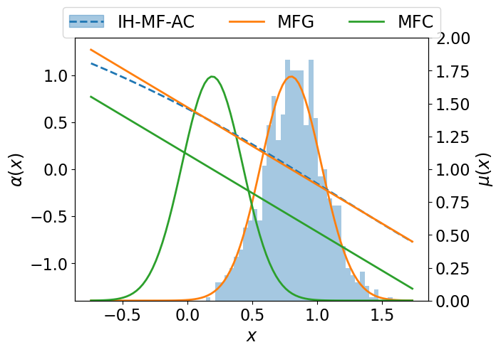
(a) Result for $\rho_{\Sigma}=10^{-6}$

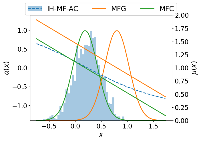
(b) Result for $\rho_{\Sigma}=5\times 10^{-4}$

Figure 1: The histogram (grey) is the learned asymptotic distribution using samples generated from the parameterized score function $\Sigma_{\varphi_{N}}$ and the dashed line (blue) is the learned feedback control after $N=10^{6}$ iterations. The green curves correspond to the optimal control and mean field distribution for MFC, while the orange curves are the equivalent for MFG. The $x$-axis shows the state variable $x$, the left $y$-axis refers to the value of the control $\alpha(x)$, and the right axis represents the probability density of $\mu(x)$.

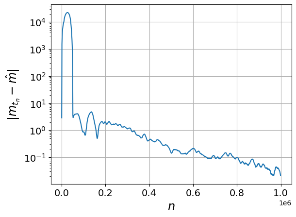
(c) Results for $\rho_{\Sigma}=10^{-6}$

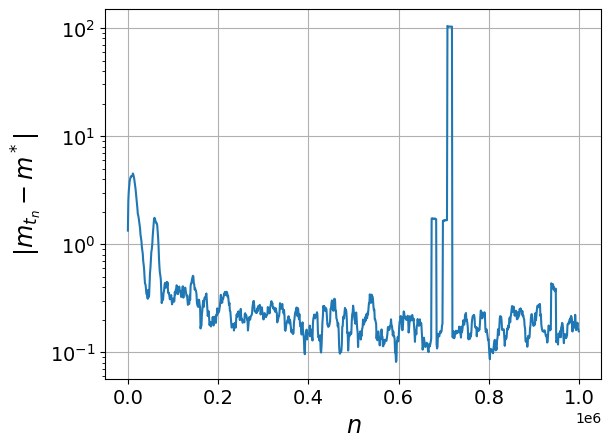
(d) Results for $\rho_{\Sigma}=5\times 10^{-4}$

Figure 2: The blue curve is a rolling average of the absolute error between the mean of samples produced from the parameterized score function $\Sigma_{\varphi_{n}}$ and the optimal mean $\hat{m}$ from eq. 5.5 in the case of MFG (left) and $m^{*}$ from eq. 5.8 in the case of MFC (right). Large jumps are due to random outliers which result from the stochasticity of our algorithm.

Table 4: Running cost coefficients and volatility for eqs. 5.1 and 5.2. The results for this parameter set are displayed in figs. 4 and 4.

$c_{1}$	$c_{2}$	$c_{3}$	$c_{4}$	$c_{5}$	$\sigma$
0.15	1.0	0.25	1.0	2.0	0.5

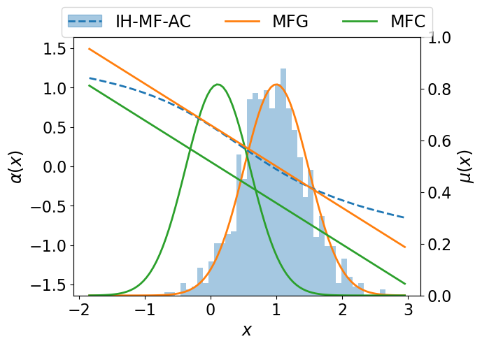
(a) MFG results for $\rho_{\Sigma}=10^{-6}$

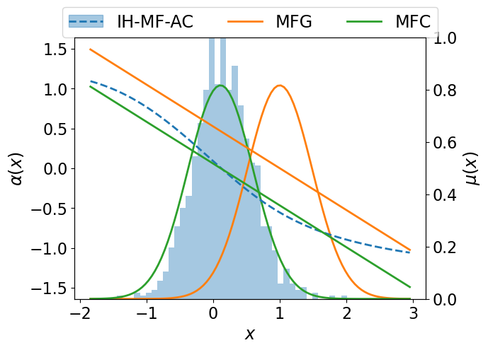
(b) MFC results for $\rho_{\Sigma}=5\times 10^{-4}$

Figure 3: The histogram (grey) is the learned asymptotic distribution using samples generated from $\Sigma_{\varphi_{n}}$ and the dashed line (blue) is the learned feedback control after $N=10^{6}$ iterations. The green curves correspond to the optimal control and mean field distribution for MFC, while the orange curves are the equivalent for MFG. The $x$-axis shows the state variable $x$, the left $y$-axis refers to the value of the control $\alpha(x)$, and the right axis represents the probability density of $\mu(x)$.

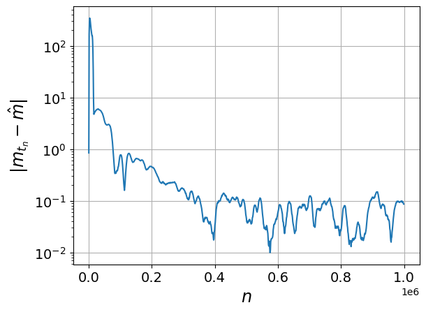
(c) Results for $\rho_{\Sigma}=10^{-6}$

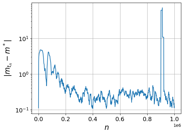
(d) Results for $\rho_{\Sigma}=5\times 10^{-4}$

Figure 4: The blue curve is a rolling average of the absolute error between the mean of samples produced from the parameterized score function $\Sigma_{\varphi_{n}}$ and the optimal mean $\hat{m}$ from eq. 5.5 in the case of MFG (left) and $m^{*}$ from eq. 5.8 in the case of MFC (right). Large jumps are due to random outliers which result from the stochasticity of our algorithm.

6 Actor-Critic Algorithm for Mean Field Control Games (MFCG)

As observed in [Angiuli et al., 2023a] in the case of tabular Q-learning, our IH-MF-AC algorithm (Algorithm 1) can easily be extended to the case of mixed mean field control game problems that involve two population distributions, a local one and a global one. This type of game corresponds to competitive games between a large number of large collaborative groups of agents. The local distribution is the “representative" agent’s group distribution, while the global distribution is the distribution of the entire population. We refer to [Angiuli et al., 2023a, Angiuli et al., 2022a] for further details on MFCG, including the limit from finite player games to infinite player games. Note that the solution gives an approximation of the Nash equilibrium between the competitive groups.

The solution of an infinite horizon mean field control game is a control-mean field pair $(\hat{\alpha},\hat{\mu})\in\mathbb{A}\times\mathcal{P}(\mathbb{R}^{d})$ satisfying the following:

1. $\hat{\alpha}$ solves the McKean-Vlasov stochastic optimal control problem

   $$\inf_{\alpha\in\mathbb{A}}J_{\hat{\mu}}(\alpha)=\inf_{\alpha\in\mathbb{A}}\mathbb{E}\left[\int_{0}^{\infty}e^{-\beta t}f\left(X_{t}^{\alpha,\hat{\mu}},\hat{\mu},\mu^{\alpha,\hat{\mu}},\alpha(X_{t}^{\alpha,\hat{\mu}})\right)\,\mathrm{d}t\right],\quad\beta>0,$$ (6.1)

   subject to

   $$\mathrm{d}X_{t}^{\alpha,\hat{\mu}}=b\left(X_{t}^{\alpha,\hat{\mu}},\hat{\mu},\mu^{\alpha,\hat{\mu}},\alpha(X_{t}^{\alpha,\hat{\mu}})\right)\,\mathrm{d}t+\sigma\left(X_{t}^{\alpha,\hat{\mu}},\hat{\mu},\mu^{\alpha,\hat{\mu}},\alpha(X_{t}^{\alpha,\hat{\mu}})\right)\,\mathrm{d}W_{t},\quad X_{0}^{\alpha,\hat{\mu}}=\xi,$$ (6.2)

   where $\mu^{\alpha,\hat{\mu}}=\lim_{t\rightarrow\infty}\mathcal{L}(\mathrm{X}_{t}^{\alpha,\hat{\mu}})$;

2. fixed point condition: $\hat{\mu}=\lim_{t\to\infty}\mathcal{L}(X_{t}^{\hat{\alpha},\hat{\mu}})$.

Note that conditions 1 and 2 above imply that $\hat{\mu}=\mu^{\hat{\alpha},\hat{\mu}}$.

We modify Algorithm 1 into our infinite horizon mean field control game actor-critic (IH-MFCG-AC) algorithm such that the global score function $\Sigma_{\varphi}$ represents the global distribution $\hat{\mu}$ and the local score function $\widetilde{\Sigma}_{\xi}$ represents the local distribution $\mu^{\alpha,\hat{\mu}}$. This is meant to mimic the parallel between the mean field game solution with the global distribution, and the mean field control solution with the local distribution. Following our intuition from Section 4.2, our choice of the now four learning rates will be chosen according to

$$\rho_{\Sigma}<\min\{\rho_{\Pi},\rho_{V}\}<\max\{\rho_{\Pi},\rho_{V}\}<\rho_{\widetilde{\Sigma}}.$$ (6.3)

Refer to Algorithm 2 for the complete pseudocode.

Algorithm 2 IH-MFCG-AC: Infinite Horizon Mean Field Control Game Actor-Critic
Differences from Algorithm 1 are highlighted in blue.

0:  Initial distribution $\xi$; number of time steps $N\gg 0$; discrete time step size $\Delta t$; neural network learning rates for actor $\rho_{\Pi}$, critic $\rho_{V}$, global score $\rho_{\Sigma}$, and local score $\rho_{\widetilde{\Sigma}}$; Langevin dynamics step size $\epsilon$.

1:  Initialize neural networks:Actor $\Pi_{\psi_{0}}:\mathbb{R}^{d}\to\mathcal{P}(\mathbb{R}^{k})$Critic $V_{\theta_{0}}:\mathbb{R}^{d}\to\mathbb{R}$Global Score $\Sigma_{\varphi_{0}}:\mathbb{R}^{d}\to\mathbb{R}^{d}$Local Score $\widetilde{\Sigma}_{\xi_{0}}:\mathbb{R}^{d}\to\mathbb{R}^{d}$

2:  Sample $X_{t_{0}}\sim\xi$

3:  for $n=0,\dots,N-1$ do

4:     Compute score loss for $\Sigma$: $\quad L_{\Sigma}(\varphi_{n})=\operatorname{tr}\left(\nabla_{x}\Sigma_{\varphi_{n}}(X_{t_{n}})\right)+\frac{1}{2}\left\lVert\Sigma_{\varphi_{n}}(X_{t_{n}})\right\rVert_{2}^{2}$

5:     Update $\Sigma$ with SGD: $\quad\varphi_{n+1}=\varphi_{n}-\rho_{\Sigma}\nabla_{\varphi}L_{\Sigma}(\varphi_{n})$

6:     Compute score loss for $\widetilde{\Sigma}$: $\quad L_{\widetilde{\Sigma}}(\xi_{n})=\operatorname{tr}\left(\nabla_{x}\widetilde{\Sigma}_{\xi_{n}}(X_{t_{n}})\right)+\frac{1}{2}\left\lVert\widetilde{\Sigma}_{\xi_{n}}(X_{t_{n}})\right\rVert_{2}^{2}$

7:     Update $\widetilde{\Sigma}$ with SGD: $\quad\xi_{n+1}=\xi_{n}-\rho_{\widetilde{\Sigma}}\nabla_{\xi}L_{\widetilde{\Sigma}}(\xi_{n})$

8:     Generate mean field samples $S_{t_{n}}=\left(S_{t_{n}}^{(1)},S_{t_{n}}^{(2)},\dots,S_{t_{n}}^{(k)}\right)$ from $\Sigma_{\varphi_{n+1}}$ and $\widetilde{S}_{t_{n}}=\left(\widetilde{S}_{t_{n}}^{(1)},\widetilde{S}_{t_{n}}^{(2)},\dots,\widetilde{S}_{t_{n}}^{(k)}\right)$ from $\widetilde{\Sigma}_{\xi_{n+1}}$ using Langevin dynamics (eq. 4.3) with step size $\epsilon$ and compute $\overline{\mu}_{S_{t_{n}}}\coloneqq\frac{1}{k}\sum_{i=1}^{k}\delta_{S_{t_{n}}^{(i)}}$ and $\overline{\mu}_{\widetilde{S}_{t_{n}}}\coloneqq\frac{1}{k}\sum_{i=1}^{k}\delta_{\widetilde{S}_{t_{n}}^{(i)}}$.

9:     Sample action: $\quad A_{t_{n}}\sim\Pi_{\psi_{n}}(\cdot\mid X_{t_{n}})$

10:     Observe reward from the environment: $\quad r_{n+1}=-f(X_{t_{n}},\overline{\mu}_{S_{t_{n}}},\overline{\mu}_{\widetilde{S}_{t_{n}}}A_{t_{n}})\Delta t$

11:     Observe next state from environment:$\quad X_{t_{n+1}}=b(X_{t_{n}},\overline{\mu}_{S_{t_{n}}},A_{t_{n}})\Delta t+\sigma(X_{t_{n}},\overline{\mu}_{S_{t_{n}}},A_{t_{n}})\sqrt{\Delta t}\,z_{n},\qquad z_{n}\sim\mathcal{N}(0,1)$

12:     Compute TD target: $\quad y_{n+1}=r_{n+1}+e^{-\beta\Delta t}V_{\theta_{n}}(X_{t_{n+1}})$

13:     Compute TD error: $\quad\delta_{\theta_{n}}=y_{n+1}-V_{\theta_{n}}(X_{t_{n}})$

14:     Compute critic loss: $\quad L_{V}(\theta_{n})=\delta_{\theta_{n}}^{2}$

15:     Update critic with SGD: $\quad\theta_{n+1}=\theta_{n}-\rho_{V}\nabla_{\theta}L_{V}(\theta_{n})$

16:     Compute actor loss: $\quad L_{\Pi}(\psi_{n})=-\delta_{\theta_{n}}\log\Pi_{\psi_{n}}(A_{t_{n}}\mid X_{t_{n}})$

17:     Update actor with SGD: $\quad\psi_{n+1}=\psi_{n}-\rho_{\Pi}\nabla_{\psi}L_{\Pi}(\psi_{n})$

18:  end for

19:  return  $(\Pi_{\psi_{N}},\Sigma_{\varphi_{N}},\widetilde{\Sigma}_{\xi_{N}})$

6.1 A Linear-Quadratic Benchmark

We test Algorithm 2 on the following linear-quadratic MFCG. We wish to minimize

$$\begin{split}\mathbb{E}\Biggl{[}\int_{0}^{\infty}e^{-\beta t}\biggl{(}\frac{1}{2}\alpha_{t}^{2}+c_{1}\left(\mathrm{X}_{t}^{\alpha,\mu}-c_{2}m\right)^{2}+c_{3}\left(\mathrm{X}_{t}^{\alpha,\mu}-c_{4}\right)^{2}\\ \quad{}+\tilde{c}_{1}\left(\mathrm{X}_{t}^{\alpha,\mu}-\tilde{c}_{2}m^{\alpha,\mu}\right)^{2}+\tilde{c}_{5}\left(m^{\alpha,\mu}\right)^{2}\biggr{)}\mathrm{d}t\Biggr{]}\end{split}$$ (6.4)

subject to the dynamics

$$\mathrm{d}X_{t}^{\alpha,\mu}=\alpha_{t}\,\mathrm{d}t+\sigma\,\mathrm{d}W_{t},\qquad t\in[0,\infty)$$ (6.5)

where $m=\int x\,\mathrm{d}\mu(x)$ and $m^{\alpha,\mu}=\int x\,\mathrm{d}\mu^{\alpha,\mu}(x)$ and the fixed point condition $m=\lim_{t\rightarrow\infty}\mathbb{E}(X_{t}^{\hat{\alpha},\mu})=m^{\hat{\alpha},\mu}$ where $\hat{\alpha}$ is the optimal action.

We present the analytic solution to the MFCG problem using notation consistent with the derivation in [Angiuli et al., 2023a]. Define

$$\Gamma_{2}=\frac{-\beta+\sqrt{\beta^{2}+8\left(c_{1}+c_{3}+\tilde{c}_{1}\right)}}{4}\qquad\text{and}\qquad\Gamma_{1}=-\frac{2\Gamma_{2}c_{3}c_{4}}{c_{1}\left(1-c_{2}\right)+\tilde{c}_{1}\left(1-\tilde{c}_{2}\right)^{2}+c_{3}+\tilde{c}_{5}}.$$

Then the optimal control for the MFCG is

$$\hat{\alpha}(x)=-(2\Gamma_{2}x+\Gamma_{1}).$$ (6.6)

Substituting eq. 6.6 into eq. 6.5 yields the Ornstein-Uhlenbeck process

$$\mathrm{d}X_{t}=-\left(2\Gamma_{2}X_{t}+\Gamma_{1}\right)\,\mathrm{d}t+\sigma\,\mathrm{d}W_{t}$$

whose limiting distribution is

$$\hat{\mu}=\mu^{\hat{\alpha},\hat{\mu}}=\mathcal{N}\left(-\frac{\Gamma_{1}}{2\Gamma_{2}},\frac{\sigma^{2}}{4\Gamma_{2}}\right).$$ (6.7)

We note that an equation for $\hat{m}$ and $m^{\hat{\alpha},\hat{\mu}}$ that only depends on the running cost coefficients is

$$m\coloneqq\hat{m}=m^{\hat{\alpha},\hat{\mu}}=\frac{c_{3}c_{4}}{c_{1}\left(1-c_{2}\right)+\tilde{c}_{1}\left(1-\tilde{c}_{2}\right)^{2}+c_{3}+\tilde{c}_{5}}.$$ (6.8)

6.2 Hyperparameters and Numerical Specifics

For the LQ benchmark problem, we consider the following choice of parameters: $c_{1}=0.5$, $c_{2}=1.5$, $c_{3}=0.5$, $c_{4}=0.25$, $\tilde{c}_{1}=0.3$, $\tilde{c}_{2}=1.25$, $\tilde{c}_{5}=0.25$, discount factor $\beta=1$, and volatility $\sigma=0.5$. The time discretization is again $\Delta t=0.01$. Our intention was to modify as few of the numerical hyperparameters from Section 5 as possible, including the neural network architectures for the actor and critic. The global and local score networks both inherit the architecture from the score network described in Section 5.4 and Table 2. The learning rates for the networks are taken directly from Table 1 with the global and score network learning rates assuming the values used to obtain the MFG and MFC results, respectively, from Section 5.4. This is to say, $(\rho_{\Pi},\rho_{V},\rho_{\Sigma},\rho_{\widetilde{\Sigma}})=(5\times 10^{-6},10^{-5},10^{-6},5\times 10^{-4}$), which satisfy $\rho_{\Sigma}<\rho_{\Pi}<\rho_{V}<\rho_{\widetilde{\Sigma}}$, the learning rate inequality proposed in eq. 6.3. The global and local distribution samples are computed at each time step using Langevin dynamics with $\epsilon=5\times 10^{-2}$ for 200 iterations using $k=1000$ samples.

The results of the IH-MFCG-AC algorithm (Algorithm 2) are presented in figs. 6 and 6. As expected, the learning of the global and local distributions reflects that of the optimal MFG distribution and the optimal MFC distribution, respectively. We observe that the global score is learned faster and with more accuracy than the local score, which is prone to outliers and instability. The optimal control is learned well within the support of the optimal distribution, but could possibly be expanded with a more advanced exploration strategy.

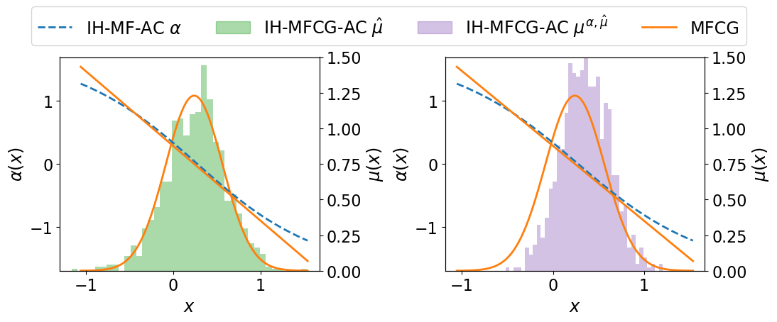
Figure 5: The histograms are the learned distributions generated using samples from the global score $\Sigma_{\varphi_{n}}$ (green) representing the global distribution $\hat{\mu}$ and the local score $\widetilde{\Sigma}_{\xi_{n}}$ (purple) representing the local score $\mu^{\alpha,\hat{\mu}}$ after $N=2\times 10^{6}$ iterations. The dashed line (blue) is the learned feedback control. The benchmark solution to the MFCG is provided in orange. The $x$-axis shows the state variable $x$, the left $y$-axis refers to the value of the control $\alpha(x)$, and the right axis represents the probability density of $\mu(x)$.

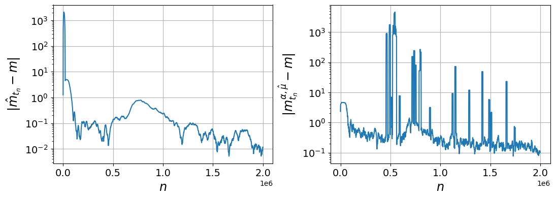
Figure 6: The blue curve is a rolling average of the absolute error of the mean of samples produced from the global score function $\Sigma_{\varphi_{n}}$ (left)—denoted $\hat{m}_{t_{n}}$—and the local score function $\widetilde{\Sigma}_{\xi_{n}}$—denoted $m^{\alpha,\hat{\mu}}_{t_{n}}$—compared to the optimal mean $m$ from eq. 6.8. Large jumps are due to random outliers which result from the stochasticity of our algorithm.

7 Conclusion

We have introduced a novel AC algorithm for solving infinite horizon mean field games and mean field control problems in continuous spaces. This algorithm, called IH-MF-AC, uses neural networks to parameterize a policy and value function, from which an optimal control is derived, as well as a score function, which represents the optimal mean field distribution on a continuous space. The MFG or MFC solution is arrived at depending on the choice of learning rates for the actor, critic, and score networks. We test our algorithm against a linear-quadratic benchmark problem and are able to recover the analytic solutions with a high degree of accuracy. Finally, we propose and test a modification of the algorithm, called IH-MFCG-AC, to solve the recently developed mixed mean field control game problems.

References

- [Angiuli et al., 2022a] Angiuli, A., Detering, N., Fouque, J.-P., Laurière, M., and Lin, J. (2022a). Reinforcement learning for intra-and-inter-bank borrowing and lending mean field control game. In Proceedings of the Third ACM International Conference on AI in Finance, ICAIF ’22, page 369–376, New York, NY, USA. Association for Computing Machinery.
- [Angiuli et al., 2023a] Angiuli, A., Detering, N., Fouque, J.-P., Laurière, M., and Lin, J. (2023a). Reinforcement learning algorithm for mixed mean field control games. Journal of Machine Learning, 2(2):108–137.
- [Angiuli et al., 2023b] Angiuli, A., Fouque, J.-P., Hu, R., and Raydan, A. (2023b). Finite horizon deep reinforcement learning for mean field problems in continuous spaces. In preparation.
- [Angiuli et al., 2022b] Angiuli, A., Fouque, J.-P., and Laurière, M. (2022b). Unified reinforcement Q-learning for mean field game and control problems. Mathematics of Control, Signals, and Systems, 34(2):217–271.
- [Angiuli et al., 2023c] Angiuli, A., Fouque, J.-P., and Laurière, M. (2023c). Reinforcement Learning for Mean Field Games, with Applications to Economics, page 393–425. Cambridge University Press.
- [Angiuli et al., 2023d] Angiuli, A., Fouque, J.-P., Laurière, M., and Zhang, M. (2023d). Accuracy of multi-scale reinforcement Q-learning algorithms for mean field game and control problems. In preparation.
- [Angiuli et al., 2019] Angiuli, A., Graves, C., Li, H., Chassagneux, J.-F., Delarue, F., and Carmona, R. (2019). CEMRACS 2017: Numerical probabilistic approach to MFG. ESAIM: ProcS, 65:84–113.
- [Borkar, 1997] Borkar, V. S. (1997). Stochastic approximation with two time scales. Systems & Control Letters, 29(5):291–294.
- [Borkar, 2008] Borkar, V. S. (2008). Stochastic Approximation: A Dynamical Systems Viewpoint. Cambridge University Press.
- [Carmona, 2020] Carmona, R. (2020). Applications of mean field games in financial engineering and economic theory. In Delarue, F., editor, Mean Field Games, volume 78 of Proceedings of Symposia in Applied Mathematics. American Mathematical Society.
- [Carmona and Delarue, 2018] Carmona, R. and Delarue, F. (2018). Probabilistic Theory of Mean Field Games with Applications I-II. Springer, United States.
- [Carmona et al., 2015] Carmona, R., Fouque, J., and Sun, L. (2015). Mean field games and systemic risk. Communications in Mathematical Sciences, 13(4):911–933. Publisher Copyright: © 2015 International Press.
- [Carmona and Laurière, 2021] Carmona, R. and Laurière, M. (2021). Deep Learning for Mean Field Games and Mean Field Control with Applications to Finance. arXiv preprint arXiv:2107.04568.
- [Carmona et al., 2021] Carmona, R., Laurière, M., and Tan, Z. (2021). Model-free mean-field reinforcement learning: Mean-field MDP and mean-field Q-learning.
- [Degris et al., 2012] Degris, T., White, M., and Sutton, R. S. (2012). Off-policy actor-critic. Proceedings of the 29th International Conference on Machine Learning.
- [Frikha et al., 2023] Frikha, N., Germain, M., Laurière, M., Pham, H., and Song, X. (2023). Actor-critic learning for mean-field control in continuous time.
- [Guo et al., 2019] Guo, X., Hu, A., Xu, R., and Zhang, J. (2019). Learning mean-field games. In Wallach, H., Larochelle, H., Beygelzimer, A., d'Alché-Buc, F., Fox, E., and Garnett, R., editors, Advances in Neural Information Processing Systems, volume 32. Curran Associates, Inc.
- [Huang et al., 2006] Huang, M., Malhamé, R. P., and Caines, P. E. (2006). Large population stochastic dynamic games: closed-loop McKean-Vlasov systems and the Nash certainty equivalence principle. Communications in Information & Systems, 6(3):221 – 252.
- [Hyvärinen, 2005] Hyvärinen, A. (2005). Estimation of non-normalized statistical models by score matching. Journal of Machine Learning Research, 6(24):695–709.
- [Jia and Zhou, 2022a] Jia, Y. and Zhou, X. Y. (2022a). Policy evaluation and temporal-difference learning in continuous time and space: A martingale approach. Journal of Machine Learning Research, 23(154):1–55.
- [Jia and Zhou, 2022b] Jia, Y. and Zhou, X. Y. (2022b). Policy gradient and actor-critic learning in continuous time and space: Theory and algorithms. Journal of Machine Learning Research, 23(275):1–50.
- [Jia and Zhou, 2023] Jia, Y. and Zhou, X. Y. (2023). Q-learning in continuous time.
- [Kingma and Ba, 2015] Kingma, D. P. and Ba, J. (2015). Adam: A method for stochastic optimization. In Bengio, Y. and LeCun, Y., editors, 3rd International Conference on Learning Representations, ICLR 2015, San Diego, CA, USA, May 7-9, 2015, Conference Track Proceedings.
- [Konda and Tsitsiklis, 2003] Konda, V. R. and Tsitsiklis, J. N. (2003). On actor-critic algorithms. SIAM Journal on Control and Optimization, 42(4):1143–1166.
- [Lasry and Lions, 2007] Lasry, J.-M. and Lions, P.-L. (2007). Mean field games. Japanese Journal of Mathematics, 2(1):229–260.
- [Laurière et al., 2022] Laurière, M., Perrin, S., Girgin, S., Muller, P., Jain, A., Cabannes, T., Piliouras, G., Perolat, J., Elie, R., Pietquin, O., and Geist, M. (2022). Scalable deep reinforcement learning algorithms for mean field games. In Chaudhuri, K., Jegelka, S., Song, L., Szepesvari, C., Niu, G., and Sabato, S., editors, Proceedings of the 39th International Conference on Machine Learning, volume 162 of Proceedings of Machine Learning Research, pages 12078–12095. PMLR.
- [Malhamé and Graves, 2020] Malhamé, R. P. and Graves, C. (2020). Mean field games: A paradigm for individual-mass interactions. In Delarue, F., editor, Mean Field Games, volume 78 of Proceedings of Symposia in Applied Mathematics. American Mathematical Society.
- [McKean, 1966] McKean, H. P. (1966). A class of markov processes associated with nonlinear parabolic equations. Proceedings of the National Academy of Science, 56:1907–1911.
- [McKean, 1967] McKean, H. P. (1967). Propagation of chaos for a class of nonlinear parabolic equations. Lecture Series in Differential Equations, 7:41–57.
- [Mnih et al., 2016] Mnih, V., Badia, A. P., Mirza, M., Graves, A., Lillicrap, T., Harley, T., Silver, D., and Kavukcuoglu, K. (2016). Asynchronous methods for deep reinforcement learning. In Balcan, M. F. and Weinberger, K. Q., editors, Proceedings of The 33rd International Conference on Machine Learning, volume 48 of Proceedings of Machine Learning Research, pages 1928–1937, New York, New York, USA. PMLR.
- [Perrin et al., 2021] Perrin, S., Laurière, M., Pérolat, J., Geist, M., Élie, R., and Pietquin, O. (2021). Mean field games flock! the reinforcement learning way. In Zhou, Z.-H., editor, Proceedings of the Thirtieth International Joint Conference on Artificial Intelligence, IJCAI-21, pages 356–362. International Joint Conferences on Artificial Intelligence Organization.
- [Rezende and Mohamed, 2015] Rezende, D. J. and Mohamed, S. (2015). Variational inference with normalizing flows. In Proceedings of the 32nd International Conference on International Conference on Machine Learning - Volume 37, ICML’15, page 1530–1538. JMLR.org.
- [Song and Ermon, 2019] Song, Y. and Ermon, S. (2019). Generative modeling by estimating gradients of the data distribution. In Wallach, H., Larochelle, H., Beygelzimer, A., d'Alché-Buc, F., Fox, E., and Garnett, R., editors, Advances in Neural Information Processing Systems, volume 32. Curran Associates, Inc.
- [Sutton, 1988] Sutton, R. S. (1988). Learning to predict by the methods of temporal differences. Machine Learning, 3(1):9–44.
- [Sutton and Barto, 2018] Sutton, R. S. and Barto, A. G. (2018). Reinforcement Learning: An Introduction. The MIT Press, second edition.
- [Sutton et al., 1999] Sutton, R. S., McAllester, D., Singh, S., and Mansour, Y. (1999). Policy gradient methods for reinforcement learning with function approximation. In Solla, S., Leen, T., and Müller, K., editors, Advances in Neural Information Processing Systems, volume 12. MIT Press.
- [van Hasselt, 2012] van Hasselt, H. (2012). Reinforcement Learning in Continuous State and Action Spaces, pages 207–251. Springer Berlin Heidelberg, Berlin, Heidelberg.
- [Wang et al., 2020] Wang, H., Zariphopoulou, T., and Zhou, X. Y. (2020). Reinforcement learning in continuous time and space: A stochastic control approach. Journal of Machine Learning Research, 21(198):1–34.
- [Watkins, 1989] Watkins, C. (1989). Learning From Delayed Rewards. PhD thesis, King’s College.