UMN-TH-4224/23

FTPI-MINN-23-16

Cosmological Collider Signatures
of Higgs-$R^{2}$ Inflation

Yohei Ema,^a,b Sarunas Verner^c

a	William I. Fine Theoretical Physics Institute, School of Physics and Astronomy,
	University of Minnesota, Minneapolis, MN 55455, USA
b	School of Physics and Astronomy, University of Minnesota, Minneapolis, MN 55455, USA
c	Institute for Fundamental Theory, Physics Department,
	University of Florida, Gainesville, FL 32611, USA

We study the cosmological collider signatures in the Higgs-$R^{2}$ inflation model. We consider two distinct types of signals: one originating from the inflaton coupling to Standard Model fermions and gauge bosons, and another arising from the isocurvature mode interaction with the inflaton. In the former case, we determine that the signal magnitude is likely too small for detection by upcoming probes, primarily due to suppression by both the Planck scale and slow-roll parameters. However, we provide a detailed computation of the signal which could be potentially applicable to various Higgs inflation variants. For the isocurvature mode signals, we observe that the associated couplings remain unsuppressed when the isocurvature mode is relatively light or comparable to the inflationary scale. In this case, we study the Higgs-$R^{2}$ inflation parameter space that corresponds to the quasi-single-field inflation regime and find that the signal strength could be as large as $|f_{\rm NL}|>1$, making Higgs-$R^{2}$ inflation a viable candidate for observation by future 21-cm surveys.

1 Introduction

Cosmic inflation plays a central role in modern cosmology [1, 2, 3, 4]. In its simplest form, inflation is driven by the potential energy of a slowly rolling scalar field, called the inflaton. Despite its success in explaining the cosmic microwave background (CMB) anisotropy and the seeds of the large-scale structure (LSS), the particle physics origin of the inflaton remains unknown, and unraveling its nature is one of the most important goals in modern cosmology.

Since the Higgs boson is the only elementary scalar field within the Standard Model (SM), it naturally invites speculation about its relationship to inflaton, another scalar field. The original Higgs model of inflation [9, 10, 11, 12], where the SM Higgs is associated with the inflaton, introduces a large non-minimal coupling of order $\xi\sim\mathcal{O}(10^{4})$ between the Higgs boson and the Ricci curvature scalar. As a result, the cut-off scale is lowered to $M_{P}/\xi$, where $M_{P}$ is the reduced Planck scale  [15, 16, 17, 18]. This scale is lower than the inflationary energy scale and hence it casts doubts on the validity of the model. In particular, while unitarity may be preserved during inflation due to the large Higgs field value [19, 20], it is violated by the production of longitudinal gauge bosons right after inflation during preheating [21]. This violation occurs due to the mass term arising from the target space curvature in the Einstein frame [22, 23]. Therefore, a UV-completion of Higgs inflation is necessary for understanding the inflationary dynamics until the end of preheating and reheating. Inflationary observables, such as the spectral index and the tensor-to-scalar ratio, depend on the reheating temperature via the number of e-folds of inflation, and this presents a critical issue in Higgs inflation.

Higgs-$R^{2}$ inflation introduces a squared Ricci scalar term, $R^{2}$, in the action. With an additional scalar degree of freedom—the scalaron—arising from the $R^{2}$ contribution [25, 26, 27, 28], the model remains perturbative up to $M_{P}$, as long as $\xi^{2}/\alpha\lesssim 1$, where $\alpha$ is the coefficient of $R^{2}$. This ensures that Higgs-$R^{2}$ inflation is a UV completion of Higgs inflation [29, 30]. A large value of $\alpha$ naturally arises from the renormalization group (RG) running [31, 32, 33, 34] when a non-minimal coupling $\xi$ is large. This UV-completion is best understood through the nonlinear sigma model [35, 36, 37]. In this framework, the target space encompasses the conformal mode of the metric and remains invariant under the Weyl transformation, with the scalaron identified with the sigma meson that flattens the target space of Higgs inflation.

In Higgs-$R^{2}$ inflation, the inflaton is a mixture of the Higgs and the scalaron. Consequently, the inflaton naturally couples to SM particles through both its Higgs component and the conformal factor, $\Omega$. A distinguishing feature of Higgs-$R^{2}$ inflation is that these couplings are all explicitly given, allowing for unambiguous study of their effects. Specifically, the preheating and reheating after inflation, associated with these couplings, have been thoroughly investigated in [38, 39, 40, 41, 42, 43].

In this paper, we study the cosmological signatures arising from the couplings between the inflationary sector and the SM particles during inflation. It is well known that a particle with a mass comparable to the Hubble parameter leaves a unique imprint in the squeezed limit of the non-gaussianity of the curvature perturbation when it couples to the inflatonary sector. These signals are referred to as cosmological collider signatures [44, 45, 46, 47, 48, 49, 50, 51].

In this context, SM particles are particularly interesting. In Higgs-$R^{2}$ inflation, even though the Higgs field value is typically much larger than the Hubble parameter during inflation, there still exist particles with masses as light as the Hubble parameter due to the large hierarchy of the Yukawa couplings [52, 53, 54]. Furthermore, the inflaton sector now contains multiple scalar fields, namely the Higgs and the scalaron, and the isocurvature mode could potentially give rise to additional cosmological collider signatures. Therefore, the main aim of this paper is to investigate these cosmological collider signatures arising from the SM particles. While we show that these signatures from the SM fermions and gauge bosons are too small to be observable in the near future, the isocurvature mode may produce a substantial effect, detectable by future 21 cm observations [55, 56].

The remainder of this paper is organized as follows: In Section 2, we review Higgs-$R^{2}$ inflation, with a focus on the coupling between the SM particles and the inflaton sector, as well as the isocurvature mode. We then compute the cosmological collider signatures of the SM fermions and gauge bosons in Section 3, and those of the isocurvature mode in Section 4. Finally, we summarize our findings in Section 5. We aim to keep our discussion free of technical details, focusing solely on key results, as the computations are quite involved and may obscure the main findings. Instead, all technical details are provided in the appendices. In Appendix A, we summarize the conventions and notation used throughout this paper. Subsequently, we review the covariant formalism of multi-field inflation in Appendix B. The results of this appendix are extensively used in the computation of the cosmological collider signatures of the isocurvature mode. Finally, we derive the propagators for scalars, fermions, and gauge bosons in de Sitter spacetime in Appendix C.

2 Preliminaries

In this section, we briefly review the inflationary dynamics of the Higgs-$R^{2}$ model [29, 57, 58, 59, 60]. We pay particular attention to the couplings between the inflaton field and other SM particles, as these are essential for understanding cosmological collider signatures.

2.1 Higgs-$R^{2}$ model and Weyl transformation

The action of Higgs-$R^{2}$ inflation in the Jordan frame is given by

$$S\;=\;\int d^{4}x\sqrt{-g}\left[\frac{M_{P}^{2}}{2}R\left(1+\frac{2\xi|\Phi|^{2}}{M_{P}^{2}}\right)+\alpha R^{2}+g^{\mu\nu}(D_{\mu}\Phi)^{\dagger}(D_{\nu}\Phi)-\lambda|\Phi|^{4}\right]+S_{\psi A}\,,$$ (2.1)

where $g_{\mu\nu}$ is the spacetime metric and $g$ is its determinant, $R$ is the Ricci curvature scalar, $\Phi$ represents the Higgs doublet, and $\lambda$ is the Higgs quartic coupling. The covariant derivative is defined as

$$D_{\mu}\Phi\;=\;\left(\partial_{\mu}-i\frac{g}{2}\tau^{a}W^{a}_{\mu}+i\frac{g^{\prime}}{2}B_{\mu}\right)\Phi\,,$$ (2.2)

where $W^{a}_{\mu}$ and $B_{\mu}$ are the SU(2) and U(1) gauge bosons, with $g$ and $g^{\prime}$ their gauge couplings, respectively, and $\tau^{a}$ is the Pauli matrix. Although the $R^{2}$ term induces the Higgs mass term and the cosmological constant due to the RG running, its effect is suppressed compared to the terms given above during inflation [34]. Therefore, we omit these terms in the following discussion. The matter action is given by

$$S_{\psi A}=\int d^{4}x\sqrt{-g} \left[i\bar{\psi}_{i}\not{\nabla}\psi_{i}-Y_{l}^{ij}\bar{L}_{i}\Phi l_{Rj}-Y_{d}^{ij}\bar{Q}_{i}\Phi d_{Rj}-Y_{u}^{ij}\bar{Q}_{i}\tilde{\Phi}u_{Rj}-\frac{1}{4}W_{\mu\nu}^{a}W^{a\mu\nu}-\frac{1}{4}B_{\mu\nu}B^{\mu\nu}\right]+\cdots,$$ (2.3)

where $\psi_{i}$ includes all the SM fermions, $Q_{i}$ is the left-handed quark doublet, $L_{i}$ is the left-handed lepton doublet, $u_{Ri}$ and $d_{Ri}$ are the right-handed up-type and down-type quarks, $l_{Ri}$ are the right-handed leptons, and $\tilde{\Phi}\equiv i\tau^{2}\Phi^{*}$. The Yukawa coupling matrices are given by $Y_{l}^{ij}$, $Y_{d}^{ij}$, and $Y_{u}^{ij}$, with the flavor indices $i$ and $j$. We omit the hermitian conjugate of the Yukawa interaction, as well as the gluon kinetic term and the interaction between the fermions and gauge bosons that are irrelevant to our study. The covariant derivative for fermions is given by

$$\not{\nabla}\psi=e^{\mu}_{a}\gamma^{a}\left(\partial_{\mu}+\frac{1}{4}\omega_{\mu}^{bc}\gamma_{bc}\right)\psi,$$ (2.4)

where $e_{\mu}^{a}$ is the tetrad defined by $g_{\mu\nu}=\eta_{ab}e_{\mu}^{a}e_{\nu}^{b}$, $\omega_{\mu}^{ab}$ is the spin connection, and $\gamma^{ab}\equiv\frac{1}{2}\left[\gamma^{a},\gamma^{b}\right]$ (see App. A for more details). We use the Latin characters for both the gauge indices and local Lorentz indices; however, their distinction is clear from the context.

The action (2.1) is defined in the Jordan frame. We now transform to the Einstein frame by performing a Weyl transformation, as it is more convenient for the analysis of inflation. We first introduce an auxiliary field $\tilde{\sigma}$ to extract the scalar degree of freedom from the $R^{2}$ term. In this case, the action becomes [27, 61]

$$S\;=\;\int d^{4}x\sqrt{-g}\left[\frac{M_{P}^{2}}{2}R\left(1+\frac{2\xi|\Phi|^{2}+4\tilde{\sigma}}{M_{P}^{2}}\right)-\frac{\tilde{\sigma}^{2}}{\alpha}+g^{\mu\nu}(D_{\mu}\Phi)^{\dagger}(D_{\nu}\Phi)-\lambda|\Phi|^{4}\right]+S_{\psi A}\,.$$ (2.5)

We perform the Weyl transformation by redefining the metric as

$$g_{\mu\nu}\to\Omega^{-2}g_{\mu\nu},\quad~{}\mathrm{where}~{}\quad\Omega^{2}\;=\;1+\frac{2\xi|\Phi|^{2}+4\tilde{\sigma}}{M_{P}^{2}}\,.$$ (2.6)

The Ricci scalar transforms under the Weyl transformation according to Eq. (A.4), and the action in the Einstein frame becomes

$$S\;=\;\int d^{4}x\sqrt{-g}\left[\frac{M_{P}^{2}}{2}R+\frac{1}{2}g^{\mu\nu}\partial_{\mu}\sigma\partial_{\nu}\sigma+e^{-\sqrt{\frac{2}{3}}\frac{\sigma}{M_{P}}}g^{\mu\nu}(D_{\mu}\Phi)^{\dagger}(D_{\nu}\Phi)-V(\sigma,\Phi)\right]+S_{\psi A}\,,$$ (2.7)

where the scalaron field $\sigma$ is defined as

$$\frac{\sigma}{M_{P}}\;\equiv\;\sqrt{6}\ln{\Omega}(\tilde{\sigma},\Phi)\,,$$ (2.8)

and the scalar potential is given by

$$V(\sigma,\Phi)\;=\;e^{-\sqrt{\frac{8}{3}}\frac{\sigma}{M_{P}}}\left[\lambda|\Phi|^{4}+\frac{M_{P}^{4}}{16\alpha}\left(e^{\sqrt{\frac{2}{3}}\frac{\sigma}{M_{P}}}-1-\frac{2\xi|\Phi|^{2}}{M_{P}^{2}}\right)^{2}\right]\,.$$ (2.9)

By redefining the fermions as $\psi_{i}\to\Omega^{3/2}\psi_{i}$, the matter sector action (2.3) in the Einstein frame becomes

$$S_{\psi A}\;=\;\int d^{4}x\sqrt{-g} \left[i\bar{\psi}_{i}\not{\nabla}\psi_{i}-\frac{1}{\Omega}\left(Y_{l}^{ij}\bar{L}_{i}\Phi l_{Rj}+Y_{d}^{ij}\bar{Q}_{i}\Phi d_{Rj}+Y_{u}^{ij}\bar{Q}_{i}\tilde{\Phi}u_{Rj}\right)-\frac{1}{4}W_{\mu\nu}^{a}W^{a\mu\nu}-\frac{1}{4}B_{\mu\nu}B^{\mu\nu}\right]\,,$$ (2.10)

where we only keep the terms that are relevant to our study. We work in the unitary gauge and take the Higgs doublet as $\Phi=(0,h/\sqrt{2})^{T}$. The electroweak (EW) gauge bosons are defined as

$$W_{\mu}^{\pm}=\frac{1}{\sqrt{2}}(W_{\mu}^{1}\mp iW_{\mu}^{2}),\quad Z_{\mu}=\cos\theta_{W}W_{\mu}^{3}+\sin\theta_{W}B_{\mu},\quad\sin\theta_{W}=\frac{g^{\prime}}{\sqrt{g^{2}+g^{\prime 2}}}.$$ (2.11)

The final action in the Einstein frame that we use for our analysis is given by

$$S\;=\;\int d^{4}x\sqrt{-g} \left[\frac{M_{P}^{2}}{2}R+\frac{1}{2}(\partial\sigma)^{2}+\frac{1}{2\Omega^{2}}(\partial h)^{2}-V(\sigma,h)+\bar{l}_{i}\left(i\not{\nabla}-m_{l_{i}}\right)l_{i}+\bar{u}_{i}\left(i\not{\nabla}-m_{u_{i}}\right)u_{i}\right.$$

$$\left.+\bar{d}_{i}\left(i\not{\nabla}-m_{d_{i}}\right)d_{i}-\frac{1}{2}W^{+}_{\mu\nu}W^{-\mu\nu}+{m_{W}^{2}}W^{+}_{\mu}W^{-\mu}-\frac{1}{4}Z_{\mu\nu}Z^{\mu\nu}+\frac{m_{Z}^{2}}{2}Z_{\mu}Z^{\mu}\right]\,.$$ (2.12)

Here the mass terms are the functions of $\sigma$ and $h$, and can be expressed as

$$m_{l_{i}}\;=\;\frac{y_{l_{i}}h}{\sqrt{2}\Omega}\,,\quad m_{u_{i}}\;=\;\frac{y_{u_{i}}h}{\sqrt{2}\Omega}\,,\quad m_{d_{i}}\;=\;\frac{y_{d_{i}}h}{\sqrt{2}\Omega}\,,\quad m_{W}^{2}\;=\;\frac{g^{2}h^{2}}{4\Omega^{2}}\,,\quad m_{Z}^{2}\;=\;\frac{m_{W}^{2}}{\cos^{2}\theta_{W}}\,,$$ (2.13)

and the scalar potential is given by

$$V(\sigma,h)\;=\;e^{-\sqrt{\frac{8}{3}}\frac{\sigma}{M_{P}}}\left[\frac{\lambda}{4}h^{4}+\frac{M_{P}^{4}}{16\alpha}\left(e^{\sqrt{\frac{2}{3}}\frac{\sigma}{M_{P}}}-1-\frac{\xi h^{2}}{M_{P}^{2}}\right)^{2}\right]\,.$$ (2.14)

Here, we rotate the fermions to the mass eigenbasis, making their mass matrices diagonal with eigenvalues $m_{\psi_{i}}$. As before, we keep only the terms relevant to our study. The Einstein frame action (2.1) is our starting point of the analysis. Note that the inflaton sector couples to the SM fermions and gauge bosons solely through the mass terms, that appear in the combination of $h/\Omega$ terms.

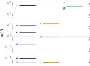
Figure 1: An example of the SM mass spectrum during inflation.

In Fig. 1, we illustrate the SM mass spectrum during inflation by solving the RG equations with SARAH [62], where the coupling values at the electroweak (EW) scale are taken from Ref. [63] (see Sec. 2.2 for the discussion of the size of the Higgs field value and the Hubble parameter during inflation). As an example, we choose the parameter $\alpha=3\times 10^{8}$ and set the RG scale to $\mu=H\simeq 1.4\times 10^{13}\,\rm{GeV}$ for this plot. We ignore the scalaron’s contribution to the runnings, as it becomes important only above the scalaron mass scale. The figure shows that even though the Higgs field value is large compared to the Hubble parameter during inflation, with $h/\Omega H\sim 2\times 10^{3}$ for our chosen parameters, the SM fermions can be as light as the Hubble parameter due to the large hierarchy between the Yukawa couplings. Consequently, these particles could produce significant cosmological collider signatures.

2.2 Inflationary predictions

Here, we review the inflationary dynamics of the Higgs-$R^{2}$ model [29, 57, 58, 59, 60]. In this model, the inflaton is a combination of the Higgs field and the scalaron, with inflation occurring in the region where $\sigma\gg M_{P}$. We use the approximation that in the Einstein frame, the inflationary potential takes a valley-like form, allowing us to use a single-field slow-roll approximation, given by [57, 58]

$$\frac{\partial V}{\partial h}\;=\;0~{}~{}\Longrightarrow~{}~{}h_{0}^{2}\;=\;\frac{\xi M_{P}^{2}}{\xi^{2}+4\lambda\alpha}\left(e^{\sqrt{\frac{2}{3}}\frac{\sigma_{0}}{M_{P}}}-1\right)\,,$$ (2.15)

where the subscript “$0$” denotes background values. Ignoring the effects of the isocurvature mode, the background action is given by

$$S_{0}\;=\;\int d^{4}x\sqrt{-g}\left[\frac{M_{P}^{2}}{2}R+\frac{1}{2}\left(1+c^{2}\right)\dot{\sigma}_{0}^{2}-\frac{\lambda M_{P}^{4}}{4(\xi^{2}+4\lambda\alpha)}\left(1-e^{-\sqrt{\frac{2}{3}}\frac{\sigma_{0}}{M_{P}}}\right)^{2}\right],\quad c^{2}\;=\;\frac{\xi}{6(\xi^{2}+4\lambda\alpha)}\,,$$ (2.16)

where terms suppressed by $e^{-\sqrt{\frac{2}{3}}\frac{\sigma_{0}}{M_{P}}}$ in the kinetic term were neglected. We focus on the parameter region where $c\lesssim 1$, necessary for a single-field slow-roll approximation as we see later. Using the principal CMB observables from the Planck analysis [65], we find that the CMB normalization fixes the parameters according to

$$\left(4\alpha+\frac{\xi^{2}}{\lambda}\right)\left(1+c^{2}\right)\;\simeq\;2.4\times 10^{9}\times\left(\frac{N_{e}}{60}\right)^{2}\,,$$ (2.17)

where $N_{e}$ represents the number of e-folds of inflation, given by

$$N_{e}\;=\;\frac{3(1+c^{2})}{4}e^{\sqrt{\frac{2}{3}}\frac{\sigma_{0}}{M_{P}}}\,,$$ (2.18)

and the spectral index and tensor-to-scalar ratio are given by

$$n_{s}\;\simeq\;1-\frac{2}{N_{e}},\qquad r\;\simeq\;\frac{12}{N_{e}^{2}}(1+c^{2})\,.$$ (2.19)

The spectral index is consistent with Planck observations [65], and the tensor-to-scalar ratio is approximately $\mathcal{O}(10^{-3})$, and within reach of future experiments like CMB-S4 [66] and LiteBIRD [67]. Furthermore, the inflationary dynamics is stable against possible Planck suppressed operators [68].

The CMB normalization (2.17) requires a large value of $\alpha$ and/or $\xi^{2}/\lambda$. If $\alpha\gg\xi^{2}/\lambda$, the inflaton is predominantly driven by the scalaron, whereas in the other case, it is primarily driven by the SM Higgs field. In the remainder of this paper, we focus on scenarios where there is no large hierarchy between $\alpha$ and $\xi^{2}/\lambda$, allowing both the Higgs and the scalaron to contribute to the inflationary sector. This requires a large value of $\xi\sim 10^{4}$, provided that the coupling $\lambda$ is not too small. While this represents the “standard” parameter region of the Higgs-$R^{2}$ model most often discussed in the literature, we also explore cases where $\xi\gg 1$ and $\xi\lesssim\mathcal{O}(0.1)$, with a small value of $\lambda$ at the inflationary scale. The latter scenario is especially important when we examine the cosmological collider signatures of the isocurvature mode.

2.3 Covariant formalism and isocurvature mode

Higgs-$R^{2}$ inflation has two scalar degrees of freedom, adiabatic and isocurvature modes. To study the mode dynamics, we use the covariant formalism of multi-field inflation [69, 70, 71, 72, 73, 74, 75]. We write down the action in the Einstein frame as

$$S\;=\;\int d^{4}x\sqrt{-g}\left[\frac{M_{P}^{2}}{2}R+\frac{1}{2}h_{ab}\partial_{\mu}\phi^{a}\partial^{\mu}\phi^{b}-V\right]\,,$$ (2.20)

where $\phi^{1}=\sigma$ and $\phi^{2}=h$. The target space metric in our case is given by

$$h_{ab}\;=\;\mathrm{diag}\left(1,e^{-\sqrt{\frac{2}{3}}\frac{\sigma}{M_{P}}}\right)\,.$$ (2.21)

The quadratic action of the curvature mode $\zeta$ and the isocurvature mode $\chi$, both of which are mixtures of the Higgs field and the scalaron, is given by

$$S_{\mathrm{quad}}\;=\;\int d^{4}xa^{3}\left[\frac{1}{2}\frac{\dot{\phi}_{0}^{2}}{H^{2}}\left(\dot{\zeta}^{2}-\frac{1}{a^{2}}\left(\partial_{i}\zeta\right)^{2}\right)+\frac{1}{2}\left(\dot{\chi}^{2}-\frac{1}{a^{2}}\left(\partial_{i}\chi\right)^{2}-m_{\chi}^{2}\chi^{2}\right)-\frac{2\dot{\theta}\dot{\phi}_{0}}{H}\dot{\zeta}\chi\right]\,.$$ (2.22)

Here, the velocity of the background field is defined as $\dot{\phi}_{0}=\sqrt{h_{ab}\dot{\phi}_{0}^{a}\dot{\phi}_{0}^{b}}$, and $\dot{\theta}$ is the turning rate that parametrizes the curvature of the inflationary trajectory, or the mixing between adiabatic and isocurvature modes. The mass of the isocurvature mode is defined as

$$m_{\chi}^{2}\;=\;N^{a}N^{b}\nabla_{b}V_{a}+\frac{\dot{\phi}_{0}^{2}}{2}\mathcal{R}-\dot{\theta}^{2},\qquad\mathcal{R}\;=\;\mathcal{R}_{ab}h^{ab}\;=\;\mathcal{R}_{acbd}h^{ab}h^{cd}\,,$$ (2.23)

with $\nabla_{a}$ and $\mathcal{R}_{acbd}$ constructed from the target space metric $h_{ab}$. Further details of the derivation are provided in Appendix B. We assume that the inflaton field value and its velocity vary along the inflationary valley, while during inflation the Higgs field evolves according to (2.15). In this case, the adiabatic and isocurvature directions are defined as

$$T^{a}\;=\;\frac{1}{\sqrt{1+c^{2}}}\begin{pmatrix}1\\ c\,e^{\sigma_{0}/\sqrt{6}M_{P}}\end{pmatrix},\quad N^{a}=\frac{1}{\sqrt{1+c^{2}}}\begin{pmatrix}-c\\ e^{\sigma_{0}/\sqrt{6}M_{P}}\end{pmatrix}\,.$$ (2.24)

We ignore terms suppressed by $1/N_{e}$ here and in subsequent discussion. By substituting the explicit forms of the target space metric and potential, we find

$$N^{a}N^{b}\nabla_{b}V_{a}\;\simeq\;\frac{\xi(24\lambda\alpha+\xi(1+6\xi))}{\lambda\alpha}H^{2},\quad\mathcal{R}=-\frac{1}{3M_{P}^{2}}\,,\quad\frac{\dot{\theta}}{H}\;\simeq\;3c\;=\;\sqrt{\frac{3\xi}{2(4\lambda\alpha+\xi^{2})}}\,.$$ (2.25)

In the standard parameter region of the Higgs-$R^{2}$ model, $\xi\gg 1$ and $\lambda\sim\mathcal{O}(0.1)$, the isocurvature mode is heavy and the turning rate is small. Consequently, the isocurvature mode can be ignored for both cosmological perturbation and cosmological collider signature studies. On the other hand, if we take the parameters as

$$\xi\sim\lambda\alpha\lesssim\mathcal{O}(0.1),$$ (2.26)

we have $m_{\chi}^{2}/H^{2}\sim\mathcal{O}(1)$ and $c\sim\mathcal{O}(0.1)$ making the isocurvature mode light and the turning rate significant. This corresponds to the so-called quasi-single field inflation regime [44, 45]. The observational effects of this regime are the main focus of Sec. 4.

2.4 Order of magnitude estimation

Before proceeding to the actual computation, we estimate the order of magnitude of cosmological collider signals arising from the SM particles. Future experiments on large-scale structure [76] and 21 cm surveys [56, 77] are expected to constrain the primordial bispectrum down to values of $f_{NL}\sim 1$, potentially probing non-Gaussianities even below this value. As previously demonstrated, the inflaton couples to SM fermions and gauge bosons via a coupling of the form $h/\Omega$. By expanding this function, we see that the coupling of the inflaton to the SM fermions and gauge bosons is of the form

$${S}_{\mathrm{int}}\;=\;\int d^{d}x\sqrt{-g}\,\mathcal{O}_{\mathrm{SM}}\left(1+c_{1}\frac{\varphi}{N_{e}M_{P}}+c_{2}\frac{\varphi^{2}}{2M_{P}^{2}}+\cdots\right)\,,$$ (2.27)

where

$$\mathcal{O}_{\mathrm{SM}}\;=\;\begin{cases}-m\bar{\psi}\psi\,,&\textrm{Fermions}\,,\\ \displaystyle\frac{m^{2}}{2}g^{\mu\nu}A_{\mu}A_{\nu}\,,&\textrm{Gauge bosons}\,,\end{cases}$$ (2.28)

and $c_{1},c_{2}$ are constants of order unity. To estimate the size of non-Gaussianity and, consequently, the signal, we first combine the linear and quadratic couplings to form the three-point function, which leads to an overall factor of $1/N_{e}M_{P}^{3}$. The non-Gaussianity scales as $f_{NL}\propto P_{\zeta}^{-2}\times H^{3}/\dot{\phi}_{0}^{3}$, where $P_{\zeta}=H^{4}/4\pi^{2}\dot{\phi}_{0}^{2}\simeq 2.1\times 10^{-9}$ is the amplitude of the power spectrum fixed by the CMB normalization. Lastly, since the coupling depends on the mass, and the cosmological collider signatures are maximized when the mass is comparable to the Hubble parameter, with $m\sim H$, we obtain a simple estimate for non-Gaussianity using dimensional analysis

$$|f_{\mathrm{NL}}|\;\lesssim\;\frac{\dot{\phi}_{0}H}{N_{e}M_{P}^{3}}\;\sim\;3.5\times 10^{3}\frac{H^{3}}{N_{e}M_{P}^{3}}\,.$$ (2.29)

Due to the suppression by the Planck scale, this value is too small to be observed by upcoming observations. Nevertheless, we rigorously compute this signal in Sec. 3 to verify the accuracy of our estimation.

As discussed in Sec. 2.3, the isocurvature mode is too heavy to leave a signal when $\xi\gg 1$. Therefore, when computing the cosmological signatures, we focus on the case $\xi\sim\lambda\alpha\lesssim 1$, which corresponds to a light isocurvature mode and the quasi-single field regime. The isocurvature mode mixes with the inflaton through the turning rate $\dot{\theta}$ and also couples to the inflaton via the potential. In particular, the derivative with respect to the isocurvature direction $N^{a}$ is not necessarily suppressed by the slow-roll parameters, and we find that the potential induces couplings of the form

$$S_{\mathrm{cubic}}\;=\;\int d\tau d^{3}x\,a^{4}\left[-\frac{1}{6}V_{N^{3}}\chi^{3}-\frac{1}{2}V_{T^{2}N}\varphi^{2}\chi\right]\,,$$ (2.30)

where $d\tau=dt/a$ is the conformal time, and

$$\frac{V_{N^{3}}}{H}\;\sim\;\frac{V_{T^{2}N}}{H}\;\sim\;\alpha^{-1/2}\,,$$ (2.31)

where we assumed $\xi\sim\lambda\alpha\sim 1$ (see Sec. 4 for the precise forms of the couplings). Since Higgs-$R^{2}$ inflation requires $\alpha\sim 10^{9}$, the couplings are relatively suppressed compared to the Hubble parameter. However, this suppression is compensated by the smallness of the power spectrum. The non-Gaussianity resulting from these couplings can be estimated as

$$f_{\mathrm{NL}}\;\sim\;\begin{cases}\displaystyle P_{\zeta}^{-1/2}\frac{V_{N^{3}}}{H}\left(\frac{\dot{\theta}}{H}\right)^{3}\,,&\textrm{for}~{}\chi^{3}\,,\vspace{1.5mm}\\ \displaystyle P_{\zeta}^{-1/2}\frac{V_{T^{2}N}}{H}\frac{\dot{\theta}}{H}\,,&\textrm{for}~{}\varphi^{2}\chi\,,\end{cases}$$ (2.32)

where the factor $P_{\zeta}^{-1/2}$ arises from the definition of the non-Gaussianity. Since $P_{\zeta}\times\alpha\sim\mathcal{O}(1)$ and the turning rate $\dot{\theta}$ can be of the order of the Hubble parameter, we expect that non-Gaussianity could potentially be as large as order unity, thus yielding an observable signature. In Sec. 4, we compute the cosmological collider signatures of the isocurvature mode in detail to confirm this expectation.

3 Cosmological collider signatures of fermions and gauge bosons

In Higgs-$R^{2}$ inflation, the inflaton naturally couples to the SM fermions and gauge bosons, potentially giving rise to cosmological collider signatures. The inflaton couples to the fermions and gauge bosons through the coupling of the form $h/\Omega$, as demonstrated in Sec. 2.1, and this coupling is expanded as

$$\frac{h}{\Omega}\;=\;\frac{h_{0}}{\Omega_{0}}+\varphi^{a}\nabla_{a}\left(\frac{h}{\Omega}\right)_{0}+\frac{1}{2}\varphi^{a}\varphi^{b}\nabla_{b}\nabla_{a}\left(\frac{h}{\Omega}\right)_{0}+\cdots\,,$$ (3.1)

where the subscript “0” indicates that the quantities are evaluated using background field values and $\varphi^{a}=\phi^{a}-\phi^{a}_{0}$. We provide technical details related to this expansion in target space in App. B. Focusing on the adiabatic direction $T^{a}$, from Eqs. (2.8) and (2.24), we obtain

$$\frac{h}{\Omega}\;\simeq\;\frac{h_{0}}{\Omega_{0}}\left(1+\sqrt{\frac{4\alpha\lambda+\xi^{2}}{24\alpha\lambda+\xi(1+6\xi)}}e^{-\sqrt{\frac{2}{3}}\frac{\sigma_{0}}{M_{P}}}\frac{\varphi}{2M_{P}}+\frac{\varphi^{2}}{12M_{P}^{2}}\right)\,,$$ (3.2)

where we only kept the leading order terms in the slow-roll expansion. In this section, we focus on the “standard” parameter region of the Higgs-$R^{2}$ model, with $\lambda\alpha\sim\xi^{2}\gg\xi$. In this limit, the above expression simplifies to

$$\frac{h}{\Omega}\;\simeq\;\frac{h_{0}}{\Omega_{0}}\left(1+\frac{\sqrt{6}}{16N_{e}}\frac{\varphi}{M_{P}}+\frac{\varphi^{2}}{12M_{P}^{2}}\right)\,,$$ (3.3)

where we used the number of e-folds $(\ref{eq:numofefolds})$. We note that the linear term is suppressed by the slow-roll parameter, or equivalently $1/N_{e}$, while the quadratic term is not suppressed. The coupling between the inflaton and SM fermions/gauge bosons is represented by the action (2.27), with $(c_{1},c_{2})=(\sqrt{6}/16,1/6)$ in the case of fermion and $(\sqrt{6}/8,1/3)$ for the gauge bosons, respectively. Here the mass $m$ is evaluated using the background field values of $\sigma$ and $h$.

In the following analysis, we evaluate the contributions of SM fermion and gauge bosons to the three-point functions. The computation is analogous to Ref. [54]. We have two contributions: one with two $\mathcal{O}_{\mathrm{SM}}$ insertions and another one with three $\mathcal{O}_{\mathrm{SM}}$ insertions. Given that the linear coupling is suppressed by an additional factor of $1/N_{e}$, our focus is on the former case. We are primarily interested in the squeezed limit of the bispectrum, with $k_{3}\ll k_{1},k_{2}$, and thus only consider the diagram containing $\hat{\varphi}_{\vec{k}_{3}}$ on the linear side and $\hat{\varphi}_{\vec{k}_{1}}\hat{\varphi}_{\vec{k}_{2}}$ on the quadratic side of the vertices. Lastly, since the cosmological collider signatures are free of UV divergences, there is no need for a regularization scheme to evaluate the diagrams. Bearing these points in mind, the diagram of interest can be expressed as follows:

$$\langle\hat{\varphi}_{\vec{k}_{1}}\hat{\varphi}_{\vec{k}_{2}}\hat{\varphi}_{\vec{k}_{3}}\rangle =\leavevmode\hbox to7.47pt{\vbox to7.47pt{\text{[drawing]}}} {\scriptstyle k_{1}~{}} {~{}~{}\scriptstyle k_{2}} {~{}~{}~{}\,\scriptstyle k_{3}} {\scriptstyle k_{1}~{}} {~{}~{}\scriptstyle k_{2}} {~{}~{}~{}\,\scriptstyle k_{3}}$$

$$=-\frac{c_{1}c_{2}}{N_{e}M_{P}^{3}}\sum_{\lambda_{1},\lambda_{2}=\pm}\lambda_{1}\lambda_{2}\int_{-\infty}^{0}\frac{d\tau_{1}d\tau_{2}}{(H^{2}\tau_{1}\tau_{2})^{4}}\Delta_{+\lambda_{1}}(k_{1};0,\tau_{1})\Delta_{+\lambda_{1}}(k_{2};0,\tau_{1})\Delta_{+\lambda_{2}}(k_{3};0,\tau_{2})$$

$$\times\int d^{3}x_{1}\,e^{-i(\vec{k}_{1}+\vec{k}_{2})\cdot\vec{x}_{1}}\int d^{3}x_{2}\,e^{-i\vec{k}_{3}\cdot\vec{x}_{2}}\langle\mathcal{O}_{SM}(\tau_{1},\vec{x}_{1})\mathcal{O}_{SM}(\tau_{2},\vec{x}_{2})\rangle_{\lambda_{1}\lambda_{2}}\,,$$ (3.4)

where the thick line indicates the asymptotic future time slice, the gray blob indicates a vertex from either the time-ordered or anti-time-ordered contours in the Schwinger-Keldysh formalism, with $\lambda_{1}$ and $\lambda_{2}$ as their corresponding labels, and the dashed lines denote the SM fermions or gauge bosons. The Schwinger-Keldysh formalism is reviewed in App. C. As the correlator depends only on $\vec{x}_{12}=\vec{x}_{1}-\vec{x}_{2}$, we can factor out the overall space integral as the delta function corresponding to momentum conservation. We define the dimensionless non-Gaussianity function $S_{\mathrm{NG}}$ as

$$\langle\zeta_{\vec{k}_{1}}\zeta_{\vec{k}_{2}}\zeta_{\vec{k}_{3}}\rangle^{\prime}\;=\;(2\pi)^{4}S_{\mathrm{NG}}(\vec{k}_{1},\vec{k}_{2},\vec{k}_{3})\frac{P_{\zeta}^{2}}{k_{1}^{2}k_{2}^{2}k_{3}^{2}}\,,$$ (3.5)

where $\zeta_{\vec{k}}=-(H/\dot{\phi}_{0})\hat{\varphi}_{\vec{k}}$ and the prime indicates that we have removed the factor $(2\pi)^{3}\delta^{(3)}(\vec{k}_{1}+\vec{k}_{2}+\vec{k}_{3})$. The SM fermion and gauge boson contribution to $S_{\mathrm{NG}}$ is expressed as

$$S_{\mathrm{NG}} =\frac{c_{1}c_{2}H\dot{\phi}_{0}}{8N_{e}M_{P}^{3}}\frac{1}{k_{1}k_{2}k_{3}}\sum_{\lambda_{1},\lambda_{2}=\pm}\lambda_{1}\lambda_{2}\int_{-\infty}^{0}\frac{d\tau_{1}d\tau_{2}}{(H^{2}\tau_{1}\tau_{2})^{4}}e^{i\lambda_{1}(k_{1}+k_{2})\tau_{1}+i\lambda_{2}k_{3}\tau_{2}}$$

$$\times\left(1-i\lambda_{1}k_{1}\tau_{1}\right)(1-i\lambda_{1}k_{2}\tau_{1})(1-i\lambda_{2}k_{3}\tau_{2})\int d^{3}x_{12}\,e^{i\vec{k}_{3}\cdot\vec{x}_{12}}\langle\mathcal{O}_{\mathrm{SM}}(\tau_{1},\vec{x}_{1})\mathcal{O}_{\mathrm{SM}}(\tau_{2},\vec{x}_{2})\rangle_{\lambda_{1}\lambda_{2}}\,,$$ (3.6)

where we used the explicit form of the massless scalar propagator $\Delta$ derived in App. C.2.

The remaining task is to evaluate the two-point function of $\mathcal{O}_{\mathrm{SM}}$. For this, we use the late-time expansion, as described in Ref. [54], to estimate the order of magnitude of the signal. In the late-time expansion, we fix $\vec{x}_{12}$ and take the limit $\tau_{1},\tau_{2}\to 0$, and different propagators become equivalent (see App. C). Therefore, we can omit the subscripts $\lambda_{1}$ and $\lambda_{2}$ from the two-point function of $\mathcal{O}_{\mathrm{SM}}$.

3.1 Fermion contribution

We first discuss the fermion contribution. As we noted above, we can drop the contour subscripts as long as we focus on the late-time behavior. Therefore, we may evaluate the two-point function as

$$\langle\mathcal{O}_{\mathrm{SM}}(\tau_{1},\vec{x}_{1})\mathcal{O}_{\mathrm{SM}}(\tau_{2},\vec{x}_{2})\rangle\;=\;-m^{2}\mathrm{Tr}\left[S(\vec{x}_{12};\tau_{1},\tau_{2})S(\vec{x}_{21};\tau_{2},\tau_{1})\right]\,,$$ (3.7)

where $\vec{x}_{21}=\vec{x}_{2}-\vec{x}_{1}$. The fermion propagator in de Sitter spacetime is given by

$$S(\vec{x}_{12};\tau_{1},\tau_{2})\;=\;\frac{H^{2}}{(4\pi)^{2}}\left[a\left(i\not{\nabla}+m\right)\right]_{1}\frac{1}{\sqrt{a_{1}a_{2}}}\left[P_{+}I_{\nu_{-}}(Z_{12})+P_{-}I_{\nu_{+}}(Z_{12})\right]\,,$$ (3.8)

where $m$ represents the fermion mass, $P_{\pm}=(1\pm\gamma^{0})/2$ is the projection operator, $a_{i}\equiv a(\tau_{i})$, $\nu_{\pm}=1/2\mp im/H$, $Z_{12}$ is the embedding distance, and the definition of $I_{\nu}(Z_{12})$ and its derivation is given in App. C.3. To take the trace, it is convenient to keep track of the projection operators $P_{\pm}$ and to write the propagators as

$$S(\vec{x}_{12};\tau_{1},\tau_{2})=\frac{H^{2}}{(4\pi)^{2}}\frac{1}{\sqrt{a_{1}a_{2}}} \left\{P_{+}\left[i\left(\partial_{\tau_{1}}+\frac{\nu_{-}-3/2}{\tau_{1}}\right)I_{\nu_{-}}(Z_{12})+i\gamma^{i}\partial_{1i}I_{\nu_{+}}(Z_{12})\right]\right.$$

$$\left.+P_{-}\left[-i\left(\partial_{\tau_{1}}+\frac{\nu_{+}-3/2}{\tau_{1}}\right)I_{\nu_{+}}(Z_{12})+i\gamma^{i}\partial_{1i}I_{\nu_{-}}(Z_{12})\right]\right\},$$ (3.9)

and

$$S(\vec{x}_{21};\tau_{2},\tau_{1})=\frac{H^{2}}{(4\pi)^{2}}\frac{1}{\sqrt{a_{1}a_{2}}} \left\{\left[i\left(\partial_{\tau_{2}}+\frac{\nu_{-}-3/2}{\tau_{2}}\right)I_{\nu_{-}}(Z_{21})+i\gamma^{i}\partial_{2i}I_{\nu_{-}}(Z_{21})\right]P_{+}\right.$$

$$\left.+\left[-i\left(\partial_{\tau_{2}}+\frac{\nu_{+}-3/2}{\tau_{2}}\right)I_{\nu_{+}}(Z_{21})+i\gamma^{i}\partial_{2i}I_{\nu_{+}}(Z_{21})\right]P_{-}\right\}.$$ (3.10)

Using these definitions, we obtain

$$\mathrm{Tr}\left[S(\vec{x}_{12};\tau_{1},\tau_{2})S(\vec{x}_{21};\tau_{2},\tau_{1})\right]$$

$$=\frac{2H^{4}}{(4\pi)^{4}}\frac{1}{a_{1}a_{2}}\left[-\left(\partial_{\tau_{1}}+\frac{\nu_{-}-3/2}{\tau_{1}}\right)I_{\nu_{-}}\left(\partial_{\tau_{2}}+\frac{\nu_{-}-3/2}{\tau_{2}}\right)I_{\nu_{-}}+(\partial_{1i}I_{\nu_{+}})(\partial_{2i}I_{\nu_{-}})+(\nu_{-}\leftrightarrow\nu_{+})\right],$$ (3.11)

where we do not distinguish between the arguments $Z_{12}$ and $Z_{21}$ as it is irrelevant for the late-time expansion. We note that the time derivative, together with the factor $\nu_{\pm}-3/2$, eliminates the leading order term in the late-time expansion of $I_{\nu_{\pm}}$. Using Eqs. (C.14) and (C.15), we evaluate the late-time expansion $Z\to\infty$ as

$$\mathrm{Tr}\left[S(\vec{x}_{12};\tau_{1},\tau_{2})S(\vec{x}_{21};\tau_{2},\tau_{1})\right]$$

$$=-\frac{H^{6}}{\pi^{4}}\frac{\frac{2\pi m}{H}(1+\frac{m^{2}}{H^{2}})}{\sinh(2\pi m/H)}(-2Z_{12})^{-3}-\frac{3H^{6}}{2\pi^{5}}\left[\Gamma\left(\nu_{-}\right)\Gamma\left(\nu_{-}-1\right)\Gamma^{2}\left(\frac{5}{2}-\nu_{-}\right)(-2Z_{12})^{-5+2\nu_{-}}+(\nu_{-}\to\nu_{+})\right],$$ (3.12)

where we ignore the terms of $\mathcal{O}(Z_{12}^{-5})$ and keep both the local and non-local contributions. We note that this result diverges from the result in [54], but we verify the consistency of our findings by considering the massless limit. If we take the limit $m\rightarrow 0$, our result simplifies to

$$\mathrm{Tr}\left[S(\vec{x}_{12};\tau_{1},\tau_{2})S(\vec{x}_{21};\tau_{2},\tau_{1})\right] \simeq-\frac{1}{\pi^{4}a_{1}^{3}a_{2}^{3}}\left[\frac{1}{x_{12}^{6}}+\frac{3(\tau_{1}-\tau_{2})^{2}}{x_{12}^{8}}+\cdots\right]\,,$$ (3.13)

where we expanded the $Z_{12}$ term. On the other hand, if $m=0$, the fermion field becomes conformal, allowing the scale factor to be factored out by redefining $\psi=a^{-3/2}\psi_{\mathrm{flat}}$. The massless fermion propagator in flat spacetime is well-known and given in coordinate space by (see e.g. [79])

$$S_{\mathrm{flat}}(x)\;=\;\frac{i\not{x}}{2\pi^{2}x^{4}}\,,$$ (3.14)

where $x$ here refers to a four-dimensional space-time coordinate. Therefore, if $m=0$, we find

$$\mathrm{Tr}\left[S(\vec{x}_{12};\tau_{1},\tau_{2})S(\vec{x}_{21};\tau_{2},\tau_{1})\right] =\frac{1}{a_{1}^{3}a_{2}^{3}}\times\mathrm{Tr}\left[S_{\mathrm{flat}}(x_{12})S_{\mathrm{flat}}(x_{21})\right]=-\frac{1}{\pi^{4}a_{1}^{3}a_{2}^{3}}\left[\frac{1}{x_{12}^{6}}+\frac{3(\tau_{1}-\tau_{2})^{2}}{x_{12}^{8}}+\cdots\right],$$ (3.15)

which coincides with our result. Focusing on the non-local part and keeping only the leading-order term, we obtain

$$\langle\mathcal{O}_{SM}(\tau_{1},\vec{x}_{1})\mathcal{O}_{SM}(\tau_{2},\vec{x}_{2})\rangle \simeq\frac{3H^{6}m^{2}}{2\pi^{5}}\left[\Gamma\left(\nu_{-}\right)\Gamma\left(\nu_{-}-1\right)\Gamma^{2}\left(\frac{5}{2}-\nu_{-}\right)\left(\frac{\tau_{1}\tau_{2}}{x_{12}^{2}}\right)^{5-2\nu_{-}}+(\nu_{-}\to\nu_{+})\right]\,.$$ (3.16)

After performing the Fourier transformation and conformal time integrals, the non-Gaussianity function in the squeezed limit $k_{3}\ll k_{1},k_{2}$ can be expressed as

$$S_{\mathrm{NG}}\;=\;-\frac{3c_{1}c_{2}H\dot{\phi}_{0}}{8\pi^{4}N_{e}M_{P}^{3}}\frac{m^{2}}{H^{2}}C_{1/2}(\nu_{-})\left(\frac{k_{3}}{k_{1}}\right)^{4-2\nu_{-}}+(\nu_{-}\to\nu_{+})\,,$$ (3.17)

where

$$C_{1/2}(\nu)\;=\;2^{2\nu}(3-\nu)(3-2\nu)^{2}\sin^{2}(\nu\pi)\sin(2\nu\pi)\Gamma(\nu)\Gamma(\nu-1)\Gamma(-8+4\nu_{-})\Gamma^{2}\left(\frac{5}{2}-\nu\right)\Gamma^{2}(2-2\nu)\,.$$ (3.18)

The coefficient $(m^{2}/H^{2})C_{1/2}(\nu_{\pm})$ peaks at $m\sim 0.1H$ and is generally of order unity. This expression aligns with our earlier estimation (2.29), albeit with an additional suppression factor $\sim(2\pi)^{-4}$ arising from the loops. Unfortunately, mainly due to Planck scale suppression, the signal is too small to be observable in the foreseeable future.

3.2 Gauge boson contribution

We next compute the contribution from the gauge bosons. The two-point function of $\mathcal{O}_{\mathrm{SM}}$ is given by

$$\langle\mathcal{O}_{\mathrm{SM}}(\tau_{1},\vec{x}_{1})\mathcal{O}_{\mathrm{SM}}(\tau_{2},\vec{x}_{2})\rangle\;=\;\frac{m^{4}}{2a_{1}^{2}a_{2}^{2}}\eta^{\alpha\beta}\eta^{\gamma\delta}G_{\alpha\gamma}(\vec{x}_{12};\tau_{1},\tau_{2})G_{\beta\delta}(\vec{x}_{12};\tau_{1},\tau_{2})\,,$$ (3.19)

where $m$ represents the gauge boson mass, and we again drop the contour indices. The gauge boson propagator in de Sitter spacetime is given by

$$G_{\alpha\beta}(\vec{x}_{1}-\vec{x}_{2};\tau_{1},\tau_{2}) =\frac{H^{2}}{m^{2}(4\pi)^{2}}K_{\alpha\beta}(Z_{12}),$$ (3.20)

where $Z_{12}$ is the embedding distance and

$$K_{\alpha\beta}(Z_{12}) =\left[Z_{12}I_{\nu}^{\prime\prime}+3I_{\nu}^{\prime}\right](\partial_{1\alpha}Z_{12})(\partial_{2\beta}Z_{12})+\left[(1-Z_{12}^{2})I_{\nu}^{\prime\prime}-3Z_{12}I_{\nu}^{\prime}\right]\partial_{1\alpha}\partial_{2\beta}Z_{12}\,,$$ (3.21)

with $\nu=\sqrt{1/4-m^{2}/H^{2}}$ and the primes denoting the derivatives with respect to $Z_{12}$. The full details of the derivation are given in App. C.4. The late-time behavior of the two-point function then becomes

$$\langle\mathcal{O}_{SM}(\tau_{1},\vec{x}_{1})\mathcal{O}_{SM}(\tau_{2},\vec{x}_{2})\rangle\;=\;\frac{3H^{8}}{128\pi^{5}}(1+2\nu)^{2}\Gamma^{2}\left(\frac{5}{2}-\nu\right)\Gamma^{2}(\nu)\left(\frac{\tau_{1}\tau_{2}}{x_{12}^{2}}\right)^{3-2\nu}+(\nu\to-\nu)\,,$$ (3.22)

where we focus on the non-local contribution. After performing the Fourier transformation and computing the conformal time integrals, the non-Gaussianity function $S_{\mathrm{NG}}$ becomes

$$S_{\mathrm{NG}} =-\frac{3c_{1}c_{2}}{8\pi^{4}}\frac{H\dot{\phi}_{0}}{N_{e}M_{P}^{3}}\frac{m^{4}}{H^{4}}C_{1}(\nu)\left(\frac{k_{3}}{k_{1}}\right)^{2-2\nu}+(\nu\to-\nu),$$ (3.23)

where

$$C_{1}(\nu)=2^{2\nu}(2-\nu)\sin^{2}(\nu\pi)\sin(2\nu\pi)\Gamma(-4+4\nu)\Gamma^{2}\left(\frac{5}{2}-\nu\right)\Gamma^{2}(\nu)\Gamma^{2}(-2\nu).$$ (3.24)

This expression correctly reproduces our estimation (2.29), with an additional suppression factor $\sim(2\pi)^{-4}$ arising from the loops. Similar to the fermion case, the signal is too small for near-future observation due to suppression by the Planck scale, $M_{P}$. Moreover, the gauge boson contribution is likely further suppressed exponentially by $m_{W}/H$ or $m_{Z}/H$ (see Fig. 1). Therefore, we turn our attention to the isocurvature mode signatures.

4 Cosmological collider signatures of isocurvature mode

As discussed in the previous section, the inflationary sector in Higgs-$R^{2}$ inflation naturally couples to SM fermions and gauge bosons, but the resulting cosmological collider signatures are too small for near-future detection. Therefore, in this section, we focus on the isocurvature mode. In the “standard” parameter region of Higgs-$R^{2}$ inflation, $\xi^{2}\gg 1$, the isocurvature mode is too heavy to be excited during inflation, leaving no observable signal. However, if $\lambda\ll 1$ such that $\xi\sim\lambda\alpha\lesssim\mathcal{O}(0.1)$, the isocurvature mode can be as light as the Hubble parameter to be excited during inflation. In this case, the isocurvature mode can produce a substantial cosmological collider signature, potentially detectable by future 21 cm observations [55, 56]. This serves as a concrete example of the clock signals discussed in Refs. [44, 45, 80], originating from a UV-complete model (up to the Planck scale) motivated by particle physics.

4.1 Mixed propagator

We first define a mixed propagator of the adiabatic and isocurvature modes, following Ref. [81]. The relevant part of the quadratic action is given by Eq. (2.22), where all details of the derivation can be found in App. B.3. Since the curvature mode $\zeta$ is related to $\varphi$ as $\zeta=-H\varphi/\dot{\phi}_{0}$, within the leading order of the slow-roll approximation, the action is equivalently expressed as

$$S_{\mathrm{quad}}\;\simeq\;\int d\tau d^{3}x\left[\frac{a^{2}}{2}\left({\varphi^{\prime}}^{2}-\left(\partial_{i}\varphi\right)^{2}\right)+\frac{a^{2}}{2}\left({\chi^{\prime}}^{2}-\left(\partial_{i}\chi\right)^{2}-a^{2}m_{\chi}^{2}\chi^{2}\right)+2\dot{\theta}a^{3}\varphi^{\prime}\chi\right]\,.$$ (4.1)

Ultimately, we evaluate the three-point function of the curvature perturbation at the asymptotic future where $\tau=0$. Therefore, we define the mixed propagator as

$$\left\langle{\hat{\varphi}(0,\vec{x}_{1})\hat{\chi}_{\pm}(\tau,\vec{x}_{2})}\right\rangle =\int\frac{d^{3}k}{(2\pi)^{3}}e^{i\vec{k}\cdot(\vec{x}_{1}-\vec{x}_{2})}\mathcal{G}_{\pm}(k;\tau)\,,$$ (4.2)

where the subscript $\pm$ denotes the contour on which $\chi$ resides. Using the Feynman rules of the Schwinger-Keldysh formalism, it is computed as (see App. C.2 for the discussion of scalar propagators)

$$\mathcal{G}_{\pm}(k;\tau) \equiv\leavevmode\hbox to0pt{\vbox to0pt{\text{[drawing]}}}=\leavevmode\hbox to7.47pt{\vbox to7.47pt{\text{[drawing]}}}+\leavevmode\hbox to7.47pt{\vbox to7.47pt{\text{[drawing]}}}$$

$$=2i\dot{\theta}\int_{-\infty}^{0}\frac{d\tau^{\prime}}{(-H\tau^{\prime})^{3}}\left[\partial_{\tau^{\prime}}\Delta(k;0,\tau^{\prime})\times G_{\pm+}(k;\tau,\tau^{\prime})-\partial_{\tau^{\prime}}\Delta(k;\tau^{\prime},0)\times G_{\pm-}(k;\tau,\tau^{\prime})\right]\,.$$ (4.3)

Here, the black (white) circle represents the vertex from the time-ordered (anti-time-ordered) contour, the solid line represents $\varphi$, and the dashed line indicates $\chi$. Additionally, we assume that the turning rate $\dot{\theta}$ is constant. We find that

$$\mathcal{G}_{\pm}(k;\tau) =\frac{\pi\dot{\theta}H}{4k^{3}}\mathcal{I}_{\pm}(-k\tau;\nu)\,,$$ (4.4)

where

$$\nu\;=\;\sqrt{\frac{9}{4}-\frac{m_{\chi}^{2}}{H^{2}}}\,,$$ (4.5)

and

$$\mathcal{I}_{\pm}(z;\nu)=z^{3/2} \left[-iH_{\nu}^{(1)}(z)\int_{0}^{\infty(1-i0)}\frac{dz^{\prime}}{\sqrt{z^{\prime}}}H_{\nu}^{(2)}(z^{\prime})e^{-iz^{\prime}}+iH_{\nu}^{(2)}(z)\int_{0}^{\infty(1+i0)}\frac{dz^{\prime}}{\sqrt{z^{\prime}}}H_{\nu}^{(1)}(z^{\prime})e^{iz^{\prime}}\right.$$

$$~{}\left.+iH_{\nu}^{(1)}(z)\int_{0}^{z(1\mp i0)}\frac{dz^{\prime}}{\sqrt{z^{\prime}}}{H_{\nu}^{(2)}}(z^{\prime})e^{\mp iz^{\prime}}-i{H_{\nu}^{(2)}}(z)\int_{0}^{z(1\mp i0)}\frac{dz^{\prime}}{\sqrt{z^{\prime}}}{H_{\nu}^{(1)}}(z^{\prime})e^{\mp iz^{\prime}}\right]\,,$$ (4.6)

where we explicitly show the $i\epsilon$ prescription. We note that we correctly reproduce the result from [81] by setting their $\lambda_{2}$ equal to our $2\dot{\theta}$. The integral can be evaluated analytically and is expressed in terms of the generalized hypergeometric functions ${}_{2}F_{2}$. We refer interested readers to Ref. [81] for its explicit form. We may focus on the parameter region $m_{\chi}/H>1$ hereafter since otherwise the isocurvature mode would not be sufficiently heavy, and the model is eventually turning into a multi-field inflation regime. Finally, we introduce the following asymptotic limit which is useful when considering the squeezed limit:

$$\mathcal{I}_{\pm}(z;\nu)\xrightarrow[z\to 0]{}-\frac{2}{\sqrt{\pi}}\left[\frac{2^{\nu}z^{3/2-\nu}\Gamma(\nu)}{\cos(\pi\nu/2)+\sin(\pi\nu/2)}+(\nu\to-\nu)\right]\,,$$ (4.7)

which does not depend on the choice of $\mathcal{I}_{+}$ or $\mathcal{I}_{-}$, and here we kept only the non-local contribution.

4.2 Bispectrum

Equipped with the mixed propagator, we now proceed to calculate the bispectrum arising from the isocurvature mode. The full cubic action for both the adiabatic and isocurvature modes is derived in App. B.4, but most terms are suppressed by slow-roll parameters. Therefore, we focus on the dominant cubic interactions, given by Eq. (2.30), where

$$V_{N^{3}} =N^{a}N^{b}N^{c}\nabla_{c}\nabla_{b}V_{a}\simeq\frac{(12\lambda\alpha+\xi(1+3\xi))\sqrt{\xi(24\lambda\alpha+\xi(1+6\xi)}}{\alpha\sqrt{2\lambda(4\alpha\lambda+\xi^{2})}}H\,,$$ (4.8)

$$V_{T^{2}N} =\frac{1}{3}\left(T^{a}T^{b}N^{c}+T^{a}N^{b}T^{c}+N^{a}T^{b}T^{c}\right)\nabla_{c}\nabla_{b}V_{a}\simeq\frac{\xi\sqrt{\xi(24\lambda\alpha+\xi(1+6\xi))}}{6\alpha\sqrt{2\lambda(4\alpha\lambda+\xi^{2})}}H\,.$$ (4.9)

In this expression, we only keep the terms of the leading order in $1/N_{e}$. Using the first coupling $V_{N^{3}}$, we obtain the expression

$$\left.\left\langle{\hat{\varphi}_{\vec{k}_{1}}\hat{\varphi}_{\vec{k}_{2}}\hat{\varphi}_{\vec{k}_{3}}}\right\rangle^{\prime}\right|_{N^{3}} =\leavevmode\hbox to7.47pt{\vbox to7.47pt{\text{[drawing]}}}+\leavevmode\hbox to7.47pt{\vbox to7.47pt{\text{[drawing]}}}$$

$$=-\frac{i\pi^{3}H^{3}}{64k_{2}^{3}k_{3}^{3}}\frac{V_{N^{3}}}{H}\left(\frac{\dot{\theta}}{H}\right)^{3}\int_{0}^{\infty}\frac{dz}{z^{4}}\left[\mathcal{I}_{+}(z;\nu)\mathcal{I}_{+}\left(\frac{k_{2}}{k_{1}}z;\nu\right)\mathcal{I}_{+}\left(\frac{k_{3}}{k_{1}}z;\nu\right)-\left(\mathcal{I}_{+}\to\mathcal{I}_{-}\right)\right]\,,$$ (4.10)

where the prime indicates that we have removed the factor of $(2\pi)^{3}\delta^{(3)}(\vec{k}_{1}+\vec{k}_{2}+\vec{k}_{3})$. From the second coupling, we find

$$\left.\left\langle{\hat{\varphi}_{\vec{k}_{1}}\hat{\varphi}_{\vec{k}_{2}}\hat{\varphi}_{\vec{k}_{3}}}\right\rangle^{\prime}\right|_{T^{2}N} =\leavevmode\hbox to7.47pt{\vbox to7.47pt{\text{[drawing]}}}+\leavevmode\hbox to7.47pt{\vbox to7.47pt{\text{[drawing]}}}+\mathrm{perm.}$$

$$=-\frac{i\pi H^{3}}{16k_{2}^{3}k_{3}^{3}}\frac{V_{T^{2}N}}{H}\frac{\dot{\theta}}{H}\int_{0}^{\infty}\frac{dz}{z^{4}}\,\left[(1+iz)\left(1+i\frac{k_{2}}{k_{1}}z\right)\mathcal{I}_{+}\left(\frac{k_{3}}{k_{1}}z;\nu\right)e^{-i\left(1+\frac{k_{2}}{k_{1}}\right)z}\right.$$

$$\left.~{}~{}~{}~{}~{}~{}~{}~{}~{}~{}~{}~{}~{}~{}~{}~{}~{}~{}~{}~{}~{}~{}~{}~{}~{}~{}~{}~{}~{}~{}~{}~{}~{}~{}~{}~{}~{}~{}-(1-iz)\left(1-i\frac{k_{2}}{k_{1}}z\right)\mathcal{I}_{-}\left(\frac{k_{3}}{k_{1}}z;\nu\right)e^{i\left(1+\frac{k_{2}}{k_{1}}\right)z}+\mathrm{perm.}\right],$$ (4.11)

where “perm.” indicates the permutations $k_{3}\leftrightarrow k_{1}$ and $k_{3}\leftrightarrow k_{2}$, which become negligible in the squeezed limit $k_{3}\to 0$. The first expression serves as an explicit example of contributions discussed in [44, 45], while the second corresponds to those discussed in [80]. In the squeezed limit, $k_{3}\ll k_{1},k_{2}$, these bispectra simplify to

$$\left.\left\langle{\hat{\varphi}_{\vec{k}_{1}}\hat{\varphi}_{\vec{k}_{2}}\hat{\varphi}_{\vec{k}_{3}}}\right\rangle^{\prime}\right|_{N^{3}} =\frac{2\pi H^{3}}{k_{1}^{3}k_{3}^{3}}\frac{V_{N^{3}}}{H}\left(\frac{\dot{\theta}}{H}\right)^{3}C_{N^{3}}(\nu)\left(\frac{k_{3}}{k_{1}}\right)^{3/2-\nu}+(\nu\to-\nu)\,,$$ (4.12)

where

$$C_{N^{3}}(\nu)\;=\;\frac{i\pi^{3/2}2^{\nu-6}\Gamma(\nu)}{\cos(\pi\nu/2)+\sin(\pi\nu/2)}\int_{0}^{\infty}dz\,z^{-(5/2+\nu)}\left[\mathcal{I}_{+}^{2}(z;\nu)-\mathcal{I}_{-}^{2}(z;\nu)\right]\,,$$ (4.13)

for the former coupling, and

$$\left.\left\langle{\hat{\varphi}_{\vec{k}_{1}}\hat{\varphi}_{\vec{k}_{2}}\hat{\varphi}_{\vec{k}_{3}}}\right\rangle^{\prime}\right|_{T^{2}N} =\frac{2\pi H^{3}}{k_{1}^{3}k_{3}^{3}}\frac{V_{T^{2}N}}{H}\frac{\dot{\theta}}{H}C_{T^{2}N}(\nu)\left(\frac{k_{3}}{k_{1}}\right)^{3/2-\nu}+(\nu\to-\nu)\,,$$ (4.14)

where

$$C_{T^{2}N}(\nu) =\frac{2^{\nu-4}(5-2\nu)}{\sqrt{\pi}(3+2\nu)}\Gamma(\nu)\Gamma\left(\frac{1}{2}-\nu\right)\tan\left(\frac{\pi(1-2\nu)}{4}\right)\,,$$ (4.15)

for the latter coupling. In particular, the conformal time integral can be analytically computed in the latter case. The corresponding non-Gaussianity function is given by

$$S_{\mathrm{NG}} =P_{\zeta}^{-1/2}\left[\frac{V_{N^{3}}}{H}\left(\frac{\dot{\theta}}{H}\right)^{3}C_{N^{3}}(\nu)+\frac{V_{T^{2}N}}{H}\frac{\dot{\theta}}{H}C_{T^{2}N}(\nu)\right]\left(\frac{k_{3}}{k_{1}}\right)^{1/2-\nu}+(\nu\to-\nu)\,,$$ (4.16)

where we assumed $\dot{\phi}_{0}<0$ so that $P_{\zeta}^{-1/2}=-2\pi\dot{\phi}_{0}/H^{2}$. This accurately reproduces our estimate, given by Eq. (2.32), up to the numerical coefficients $C_{N^{3}}$ and $C_{T^{2}N}$. We represent the coefficient of the non-Gaussianity function as

$$f_{\mathrm{NL}}\;=\;\frac{10}{9}P_{\zeta}^{-1/2}\left[\frac{V_{N^{3}}}{H}\left(\frac{\dot{\theta}}{H}\right)^{3}C_{N^{3}}(\nu)+\frac{V_{T^{2}N}}{H}\frac{\dot{\theta}}{H}C_{T^{2}N}(\nu)\right]\,,$$ (4.17)

which characterizes the size of the non-Gaussianity. However, when $m/H>3/2$, the coefficient $\nu$ becomes imaginary, and this quantity cannot be evaluated at the equilateral configuration.

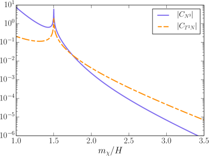
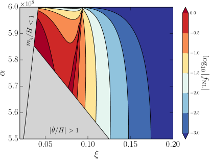
Figure 2: Left panel: $C_{N^{3}}(\nu)$ and $C_{T^{2}N}(\nu)$ as functions of $m_{\chi}/H$. Note that $\nu$ is real for $m_{\chi}/H<3/2$ and it is purely imaginary for $m_{\chi}/H>3/2$. We show only the cases where $\nu>0$ for $m_{\chi}/H<3/2$ because this contribution is less suppressed by $k_{3}/k_{1}$ in the squeezed limit. On the other hand, for $m_{\chi}/H>3/2$, the coefficients $C_{N^{3}}(-\nu)$ and $C_{T^{2}N}(-\nu)$ can be related to the complex conjugated functions $C_{N^{3}}^{*}(\nu)$ and $C_{T^{2}N}^{*}(\nu)$. Right panel: The coefficients of the non-Gaussianity function for different values of $\xi$ and $\alpha$, with $\lambda$ fixed using the CMB normalization (2.17) with $N_{e}=60$ e-folds (ignoring the $c^{2}$ contribution). The small region, where $|f_{\mathrm{NL}}|>1$ with $\xi\sim 0.08$, corresponds to $m_{\chi}/H\simeq 3/2$, and for larger $\xi$, $m_{\chi}/H>3/2$, and the signal exhibits oscillatory behavior with respect to $k_{3}/k_{1}$. We focus on the region $m_{\chi}/H>1$ and $|\dot{\theta}/H|<1$ so that the model is in the quasi-single field regime. Notably, these two conditions imply that $|\dot{\theta}/m_{\chi}|<1$.

In the left panel of Fig. 2, we display the coefficients $C_{N^{3}}(\nu)$ and $C_{T^{2}N}(\nu)$ as functions of $m_{\chi}/H$. We note that the parameter $\nu$ is real for $m_{\chi}/H<3/2$ and purely imaginary for $m_{\chi}/H>3/2$. These function are exponentially suppressed for large values of $m_{\chi}/H$, aligning with the expectation that cosmological collider signatures arise from the non-local propagation of particles. In the large mass limit $m_{\chi}\gg H$, correlation functions usually include two contributions: one power-suppressed and the other exponentially suppressed by the mass term. The former corresponds to higher-dimensional operators and gives rise only to local effects (see, for example, Refs. [82, 83]), while the latter is associated with particle production and, consequently, cosmological collider signatures.

In the right panel of Fig. 2, we show the non-Gaussianity coefficient $|f_{\mathrm{NL}}|$ as a function of $\xi$ and $\alpha$. In this figure, we set $\lambda$ according to the CMB normalization (2.17) (with $c^{2}$ ignored). As is evident from the figure, the coefficient can attain values as large as order unity while satisfying the conditions $m_{\chi}/H>1$ and $|\dot{\theta}/H|<1$, so that the model is in the quasi-single field inflation regime. Therefore, this signal is potentially detectable by future 21 cm observations [55, 56] within this specific parameter space region.

In Fig. 3, we plot the full non-Gaussianity function in the squeezed limit (4.16) for different values of $m_{\chi}/H$. Here we consider a choice of Higgs-$R^{2}$ inflation parameters in the range $0.04\lesssim\xi\lesssim 0.4$, $4\times 10^{8}\lesssim\alpha\lesssim 6\times 10^{8}$, and using the CMB normalization (2.17) (where we ignore the $c^{2}$ contribution) with $N_{e}=60$ e-folds, we determine the value of $\lambda$ and the mass of the isocurvature mode (2.23). The left panel of Fig. 2 illustrates that the signal peaks when $|C_{N^{3}}|\sim\mathcal{O}(1)$, with $m_{\chi}/H\sim 1$. However, we show in Fig. 3, that when $m_{\chi}/H>3/2$, the parameter $\nu$ becomes imaginary and the squeezed limit displays an oscillatory feature, leading to a distinct clock signal. However, this signal has a reduced non-Gaussianity amplitude compared to the $m_{\chi}\simeq H$ case. We highlight these important oscillatory features in non-Gaussianities across three panels, where $\nu$ is imaginary for the values $m_{\chi}/H=2,3,$ and $4$. For a more detailed discussion of clock signals, see Ref. [80].

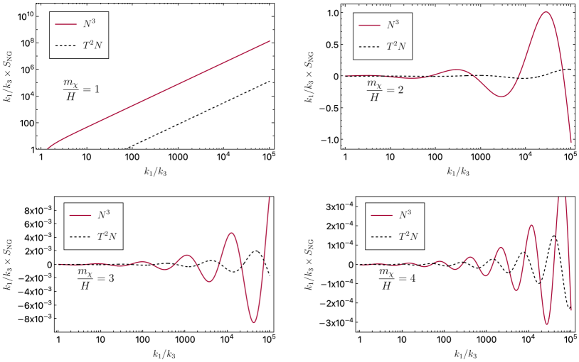
Figure 3: The non-Gaussianity function in the squeezed limit (4.16) as a function of $k_{1}/k_{3}$ for the mass range $m_{\chi}/H=1,2,3,$ and $4$ . To enhance the oscillatory components of the clock signals, we scale $S_{\rm NG}$ by a factor of $k_{1}/k_{3}$. We consider a nominal choice of the Higgs-$R^{2}$ inflation parameters in the range $0.04\lesssim\xi\lesssim 0.4$, $4\times 10^{8}\lesssim\alpha\lesssim 6\times 10^{8}$, where $\lambda$ is fixed by the CMB normalization (2.17) (where we ignore the $c^{2}$ contribution) with $N_{e}=60$ e-folds, and the mass of the isocurvature mode is determined from Eq. (2.23). Although the signal strength peaks when $m_{\chi}\sim H$ and $\nu$ is real, which maximizes the value of the coupling $|C_{N^{3}}(\nu)|$, the oscillatory behavior is only evident for the imaginary values of $\nu$, with $m_{\chi}/H=2,3,$ and $4$. The panels also illustrate that the $N^{3}$ coupling is always more significant than the $T^{2}N$ coupling.

Finally, we comment on the trispectrum. In Higgs-$R^{2}$ inflation, we find that the quartic couplings of the adiabatic and isocurvature modes are given by

$$S_{\mathrm{quartic}}\;=\;\int d\tau d^{3}x\,a^{4}\left[\frac{1}{24}V_{N^{4}}\chi^{4}+\frac{1}{4}V_{T^{2}N^{2}}\chi^{2}\varphi^{2}\right]\,,$$ (4.18)

where

$$V_{N^{4}} \simeq\frac{7+3\xi(14+9\xi)}{18\alpha}+\lambda\left(6-\frac{14}{9(\xi^{2}+4\lambda\alpha)}\right),\quad V_{T^{2}N^{2}}\simeq\frac{\xi(132\lambda\alpha+\xi(7+33\xi)}{108\alpha(\xi^{2}+4\lambda\alpha))},$$ (4.19)

with the other combinations suppressed by the slow-roll parameters. These couplings both scale as $V_{N^{4}}\sim V_{T^{2}N^{2}}\sim 1/\alpha$ for $\xi\sim\lambda\alpha\sim\mathcal{O}(1)$. Therefore, an estimation similar to Sec. 2.4 provides us with

$$g_{\mathrm{NL}},~{}\tau_{\mathrm{NL}}\sim P_{\zeta}^{-1}\frac{V_{N^{4}}}{H}\left(\frac{\dot{\theta}}{H}\right)^{4},~{}~{}P_{\zeta}^{-1}\frac{V_{T^{2}N^{2}}}{H}\left(\frac{\dot{\theta}}{H}\right)^{2}.$$ (4.20)

We expect a similar size of the signal from the combination of the cubic interactions. Since $P_{\zeta}\times\alpha\sim 1$, this can be of order unity for $\xi\sim\lambda\alpha\sim 1$, and hence we expect a sizable trispectrum in the parameter region of our interest in this section. We leave a detailed study on the trispectrum, including its precise size and spectral feature in the squeezed limit, as a possible future work.

5 Conclusions and Discussion

In this work, we examined and computed the cosmological collider signals for Higgs-$R^{2}$ inflation. We considered two distinct types of potential signals. The first originates from the inflaton coupling to the SM fermions and gauge bosons through the coupling $h/\Omega$. The second is an isocurvature mode coupling that couples to the inflaton through the turning rate $\dot{\theta}$.

We found that the cosmological collider signatures from the SM fermions and gauge bosons are relatively weak due to their Planck suppression and further suppression by slow-roll parameters, or the number of e-folds $N_{e}$. Consequently, they are unlikely to be detected even by forthcoming 21 cm probes. However, a considerably stronger signal might emerge from the isocurvature mode and inflaton couplings. In the parameter space, where $\xi\sim\lambda\alpha\sim\mathcal{O}(0.1)$, the isocurvature mode remains light, and the turning rate $\dot{\theta}$, and subsequently coupling to the inflaton, is large. This parameter region aligns with the quasi-single inflation regime of Higgs-$R^{2}$ inflation, with parameters spanning from $0.5\lesssim\xi\lesssim 2$ and $4\times 10^{8}\lesssim\alpha\lesssim 6\times 10^{8}$. Importantly, in this scenario, the non-Gaussianity could be significant, with $|f_{\rm NL}|\sim\mathcal{O}(1)$, peaking when $m_{\chi}/H\simeq 3/2$. Although the isocurvature mode contribution to $f_{\rm NL}$ is large in this parameter space, it might be difficult for future 21 cm observations to isolate it from the background. However, when $m_{\chi}/H\gtrsim 3/2$, the cubic interaction of the isocurvature mode, and consequently $f_{\rm NL}$, still remain nearly of order unity. This oscillatory clock signal might be distinguishable from the 21 cm background, offering hope for detection by future experiments.

We note that detecting a signal originating from the isocurvature mode couplings could provide strong evidence for multi-field models of inflation. The Higgs-$R^{2}$ model remains a highly appealing scenario due to several of its features, including a UV-completion. It would be interesting to explore the full features and the parameter space of a multi-field Higgs-$R^{2}$ model and its associated cosmological collider signatures. However, such a study is quite involved, and we hope to investigate it in future work.

In this paper, we only focused on the SM particles. However, once we introduce new particles, the inflaton typically couples to them through the conformal factor, $\Omega$, unless these new particles are conformal. For example, the inflaton can couple to right-handed neutrinos via the Yukawa interaction and Majorana mass terms. Our estimates from Sec. 2.4 likely remain valid in this scenario, with $c_{1},c_{2}\sim\mathcal{O}(1)$. Therefore, we do not expect that these new particles would significantly enhance the cosmological collider signatures in Higgs-$R^{2}$ inflation. The situation might change if a stronger coupling between the inflaton and the new particles is introduced, although this might spoil the UV-completeness of the model by introducing an additional scale.

Another intriguing question is if there are variants of Higgs inflation where the SM fermions and gauge bosons leave observable cosmological collider signatures. One such variant of Higgs inflation scenario, known as Palatini Higgs inflation [87, 88, 89], has recently attracted attention. This model has the same action as the original Higgs inflation model but relies on the Palatini formalism of gravity, where the spin connection and vierbein are treated independently. This model avoids the unitarity issues both during [88] and after inflation [90, 23, 91], in contrast to the metric formalism. In general, using the same arguments as in Sec. 2.4, we expect that the non-Gaussianity arising from the SM particles takes the form

$$f_{\mathrm{NL}}\;\sim\;\frac{\dot{\phi}_{0}H}{\Lambda^{3}}\sim 3.5\times 10^{3}\frac{H^{3}}{\Lambda^{3}}\,,$$ (5.1)

where $\Lambda$ is the scale of the inflaton coupling to the SM particles. In Palatini Higgs inflation, the cut-off scale is given by $\Lambda\sim M_{P}/\sqrt{\xi}$, which is significantly smaller than the Planck scale since from the CMB normalization, we find $\xi\sim 5\times 10^{10}\lambda$. However, in this model the Hubble parameter is also relatively small, with $H\sim\sqrt{\lambda}M_{P}/\xi$. Therefore, the size of non-Gaussianity can be estimated as

$$f_{\mathrm{NL}}\;\sim\;3.5\times 10^{3}\times\left(\frac{\lambda}{\xi}\right)^{3/2}\sim 10^{-13}\,,$$ (5.2)

which is too small to be observed in the near future. Nonetheless, it is still interesting to explore if there are other variants that predict a larger cosmological collider signal.

Acknowledgements —

The work of Y.E. and S.V. was performed in part at the Aspen Center for Physics, which is supported by National Science Foundation grant PHY-2210452. We would also like to thank Soubhik Kumar and Yiming Zhong for useful discussions. Y.E. is supported in part by DOE grant DE-SC0011842. The work of S.V. was supported in part by DOE grant DE-SC0022148. The Feynman diagrams in this paper are drawn with TikZ-Feynman [92].

Appendix A Conventions and notation

A.1 Conventions

Here we summarize the conventions used in this paper.

Metric sector

We take almost the plus convention,

$$\eta_{\mu\nu}\;=\;\mathrm{diag}(+1,-1,-1,-1)\,.$$ (A.1)

The geometrical quantities are defined as

$$\Gamma^{\mu}_{\nu\rho} =\frac{1}{2}g^{\mu\alpha}\left(\partial_{\nu}g_{\rho\alpha}+\partial_{\rho}g_{\nu\alpha}-\partial_{\alpha}g_{\nu\rho}\right),\quad{R_{\mu\nu\rho}}^{\sigma}=\partial_{\mu}\Gamma^{\sigma}_{\nu\rho}-\partial_{\nu}\Gamma^{\sigma}_{\mu\rho}+\Gamma^{\alpha}_{\nu\rho}\Gamma^{\sigma}_{\alpha\mu}-\Gamma^{\alpha}_{\mu\rho}\Gamma^{\sigma}_{\alpha\nu},$$ (A.2)

$$R_{\mu\nu} ={R_{\mu\alpha\nu}}^{\alpha}=\partial_{\mu}\Gamma^{\alpha}_{\alpha\nu}-\partial_{\alpha}\Gamma^{\alpha}_{\mu\nu}+\Gamma^{\alpha}_{\beta\nu}\Gamma^{\beta}_{\alpha\mu}-\Gamma^{\alpha}_{\mu\nu}\Gamma^{\beta}_{\alpha\beta},\quad R=g^{\mu\nu}R_{\mu\nu}\,.$$ (A.3)

With this definition, the sign in front of the Einstein-Hilbert action is positive, and the conformal coupling corresponds to $\xi=-1/6$. The Ricci scalar transforms under the Weyl transformation as

$${g}_{\mu\nu}\to\Omega^{-2}g_{\mu\nu},\quad{R}\to\Omega^{2}\left[R+\frac{3}{2}(\partial_{\mu}\ln\Omega^{2})(\partial^{\mu}\ln\Omega^{2})-3\Box\ln\Omega^{2}\right]\,.$$ (A.4)

Finally the commutator acting on a vector field $V^{\alpha}$ satisfies

$$[\nabla_{\mu},\nabla_{\nu}]V^{\alpha}={R_{\mu\nu\beta}}^{\alpha}V^{\beta}.$$ (A.5)

Target space sector

Since the target space metric is positive definite, we may change the sign convention from the metric sector. The Christoffel symbol is defined as

$$\Gamma^{a}_{bc}\;=\;\frac{1}{2}h^{ad}\left(h_{db,c}+h_{dc,b}-h_{bc,d}\right)\,,$$ (A.6)

and the Riemann tensor is defined as

$${\mathcal{R}^{a}}_{bcd}\;=\;\partial_{c}\Gamma^{a}_{db}-\partial_{d}\Gamma^{a}_{cb}+\Gamma^{a}_{ce}\Gamma^{e}_{db}-\Gamma^{a}_{de}\Gamma^{e}_{cb}\,,$$ (A.7)

which has the opposite sign convention from the metric sector. The Ricci tensor and Ricci scalar are defined as

$$\mathcal{R}_{ab}\;=\;h^{cd}\mathcal{R}_{acbd}\,,\quad\mathcal{R}\;=\;h^{ab}\mathcal{R}_{ab}\,.$$ (A.8)

Fermion sector

The covariant derivative in the fermion sector is given by

$$\nabla_{\mu}\psi =\left(\partial_{\mu}+\frac{1}{4}\omega_{\mu}^{ab}\gamma_{ab}\right)\psi.$$ (A.9)

We define the gamma matrices as

$$\left\{\gamma^{a},\gamma^{b}\right\} =2\eta^{ab},\quad\gamma_{ab}=\frac{1}{2}\left(\gamma_{a}\gamma_{b}-\gamma_{b}\gamma_{a}\right),\quad\gamma_{5}=i\gamma^{0}\gamma^{1}\gamma^{2}\gamma^{3}=-\frac{i}{4!}\epsilon^{abcd}\gamma_{a}\gamma_{b}\gamma_{c}\gamma_{d},$$ (A.10)

with $\epsilon^{0123}=+1$. We use $a,b,\cdots$ for the local Lorentz indices and $\mu,\nu,\cdots$ for the spacetime indices. The spin connection and the vierbein are defined as

$$\omega_{\mu}^{ab} =e^{a}_{\nu}\left[\partial_{\mu}e^{\nu b}+{\Gamma^{\nu}}_{\sigma\mu}e^{\sigma b}\right],\quad g_{\mu\nu}=e_{\mu}^{a}\eta_{ab}e_{\nu}^{b}.$$ (A.11)

Under the Weyl transformation, the fermion kinetic term transforms as

$${\not{\nabla}}{\psi}\to\Omega^{5/2}\not{\nabla}\left(\Omega^{-3/2}\psi\right)\,,$$ (A.12)

in four spacetime dimensions.

A.2 ADM decomposition

Here we may explain the $3+1$ decomposition of the Ricci scalar that we use in the computation of the perturbation. We may use the ADM decomposition [93]

$$ds^{2}\;=\;N^{2}dt^{2}-\gamma^{ij}(dx^{i}+\beta^{i}dt)(dx^{j}+\beta^{j}dt)\,,$$ (A.13)

or equivalently

$$g_{\mu\nu}\;=\;\begin{pmatrix}N^{2}-\beta^{i}\beta_{i}&-\beta_{i}\\ -\beta_{j}&-\gamma_{ij}\end{pmatrix}\,,\quad g^{\mu\nu}\;=\;\begin{pmatrix}N^{-2}&-N^{-2}\beta^{i}\\ -N^{-2}\beta^{j}&-\gamma^{ij}+N^{-2}\beta^{i}\beta^{j}\end{pmatrix}\,,$$ (A.14)

where the spatial indices $i,j$ are raised and lowered by $\gamma_{ij}$. We may define the temporal part of the vierbein $n_{\mu}$ and the extrinsic curvature $K_{\mu\nu}$ as

$$n_{\mu}\;\equiv\;(N,\vec{0}),\quad K_{\mu\nu}\;=\;\nabla_{\nu}n_{\mu}\,.$$ (A.15)

Our goal is to express the Ricci scalar in terms of $K_{\mu\nu}$ and the three-dimensional curvature tensors. For this purpose, we first take the Gauss normal coordinate, $N=1$ and $\beta^{i}=0$, and compute everything in these coordinates. We then express the result by the covariant quantities so that we can go back to the general coordinate. In the Gauss normal coordinates, we can easily show that

$$\Gamma^{0}_{00}\;=\;\Gamma^{0}_{0i}=\Gamma^{i}_{00}=0\,,\quad\Gamma^{0}_{ij}\;=\;\frac{1}{2}\dot{\gamma}_{ij}=-K_{ij}\,,\quad\Gamma^{i}_{0j}\;=\;\frac{1}{2}\gamma^{ik}\dot{\gamma}_{jk}\;=\;-{K^{i}}_{j}\,.$$ (A.16)

The Ricci scalar is decomposed as

$$R\;=\;2{R_{0\alpha 0}}^{\alpha}-\gamma^{ij}{R_{ikj}}^{k}\,.$$ (A.17)

The first term is equally expressed as

$${R_{0\alpha 0}}^{\alpha}\;=\;n^{\mu}n^{\nu}{R_{\mu\alpha\nu}}^{\alpha}=n^{\mu}[\nabla_{\mu},\nabla_{\nu}]n^{\nu}\,,$$ (A.18)

which is now in covariant form. The second term is also easily computed as

$$-\gamma^{ij}{R_{ikj}}^{k}=R^{(3)}-K_{ij}K^{ij}+K^{2},$$ (A.19)

where $K=\gamma^{ij}K_{ij}$. We further note that

$$n^{\mu}K_{\mu\rho}\;=\;n^{\mu}\nabla_{\rho}n_{\mu}=0\,.$$ (A.20)

Therefore we obtain after integration by parts

$$R\;=\;R^{(3)}+K_{ij}K^{ij}-K^{2}+(\mathrm{total}~{}\mathrm{deriv})\,,$$ (A.21)

which is the desired $3+1$ decomposition of the Ricci scalar. Following [78], we define

$$K_{ij}\;=\;-\frac{1}{N}E_{ij}\,.$$ (A.22)

In the general ADM coordinate, it is given by

$$K_{ij}\;=\;-\frac{1}{2N}\left(\dot{\gamma}_{ij}-\nabla_{j}^{(3)}\beta_{i}-\nabla_{i}^{(3)}\beta_{j}\right)\,.$$ (A.23)

Appendix B Covariant formalism of multi-field inflation

In this appendix, we review the covariant formalism of multi-field inflation [69, 70, 71, 72, 73, 74, 75].

B.1 Background dynamics

We first consider the background dynamics. We take

$$ds^{2}\;=\;N^{2}(t)dt^{2}-a^{2}(t)dx^{i}dx^{i}\,,\quad\phi^{a}\;=\;\phi^{a}_{0}(t)\,.$$ (B.1)

The Ricci scalar is given by

$$R\;=\;-\frac{6H^{2}}{N^{2}}+(\mathrm{total}~{}\mathrm{deriv}),\quad H=\frac{\dot{a}}{a}\,.$$ (B.2)

By taking the derivative of the action with respect to $\phi^{a}$, $N$, and $a$, and then setting $N=1$, we obtain

$$\mathcal{D}_{t}\dot{\phi}^{a}_{0}+3H\dot{\phi}_{0}^{a}+\partial^{a}V\;=\;0\,,\quad H^{2}\;=\;\frac{1}{3M_{P}^{2}}\left(\frac{1}{2}h_{ab}\dot{\phi}^{a}_{0}\dot{\phi}^{b}_{0}+V\right)\,,\quad\dot{H}\;=\;-\frac{1}{2M_{P}^{2}}h_{ab}\dot{\phi}_{0}^{a}\dot{\phi}_{0}^{b}\,,$$ (B.3)

where the covariant derivative is defined as

$$\mathcal{D}_{t}X^{a}\;=\;\dot{X}^{a}+\Gamma^{a}_{bc}\dot{\phi}_{0}^{b}X^{c}\,,$$ (B.4)

with $\Gamma^{a}_{bc}$ being the Christoffel symbol constructed from $h_{ab}$. We define

$$T^{a}\;\equiv\;\frac{\dot{\phi}_{0}^{a}}{\dot{\phi}_{0}}\,,\quad\mathcal{D}_{t}T^{a}\;\equiv\;-\dot{\theta}N^{a}\,,\quad\dot{\phi}_{0}\;=\;\sqrt{h_{ab}\dot{\phi}_{0}^{a}\dot{\phi}_{0}^{b}}\,,$$ (B.5)

where $T^{a}$ indicates the direction of the inflationary trajectory while $N^{a}$ the orthogonal direction with the normalization $N^{a}N_{a}=1$. The turning rate $\dot{\theta}$ parametrizes the curvature of the inflationary trajectory, or the mixing between the adiabatic and isocurvature modes as we will see. By using the equation of motion of $\phi_{0}^{a}$, we see that

$$\mathcal{D}_{t}T^{a}\;=\;-\frac{T^{a}}{\dot{\phi}_{0}}\left(\ddot{\phi}_{0}+3H\dot{\phi}_{0}+V_{\phi}\right)-\frac{1}{\dot{\phi}_{0}}\left(V^{a}-T^{a}V_{\phi}\right)\,,\quad V_{\phi}\;=\;T^{a}V_{a}\,,$$ (B.6)

where $V^{a}=\partial^{a}V$ and so on. Since $T^{a}$ is normalized, we have $T_{a}(DT^{a}/dt)=0$, from which we obtain

$$\ddot{\phi}_{0}+3H\dot{\phi}_{0}+V_{\phi} =0,\quad\dot{\theta}N^{a}=\frac{1}{\dot{\phi}_{0}}\left(V^{a}-T^{a}V_{\phi}\right)\,.$$ (B.7)

The latter tells us that

$$V_{a}\;=\;N_{a}V_{N}+T_{a}V_{\phi}\,,\quad V_{N}\;=\;N^{a}V_{a}\,,\quad\dot{\theta}\;=\;\frac{V_{N}}{\dot{\phi}_{0}}\,,\quad N^{a}\;=\;\frac{V^{a}-T^{a}V_{\phi}}{\sqrt{h_{ab}(V^{a}-T^{a}V_{\phi})(V^{b}-T^{b}V_{\phi})}}\,.$$ (B.8)

Note that $\dot{\theta}$ depends on the derivative of the potential in the $N$-direction, not in the $T$-direction, and thus this can be large during slow-roll inflation. We define the slow-roll parameters as

$$\epsilon\;=\;-\frac{\dot{H}}{H^{2}}\;=\;\frac{\dot{\phi}_{0}^{2}}{2M_{P}^{2}H^{2}}\,,\quad\eta^{a}\;=\;-\frac{1}{H\dot{\phi}_{0}}\mathcal{D}_{t}\dot{\phi}_{0}^{a}\,.$$ (B.9)

By using the equation of motion of $\phi_{0}^{a}$, we can show that

$$\eta^{a}\;=\;\eta_{\parallel}T^{a}+\eta_{\perp}N^{a},\quad\eta_{\parallel}\;=\;-\frac{\ddot{\phi}_{0}}{H\dot{\phi}_{0}}\,,\quad\eta_{\perp}\;=\;\frac{\dot{\theta}}{H}\;=\;\frac{V_{N}}{H\dot{\phi}_{0}}\,.$$ (B.10)

The slow-roll condition requires $\epsilon,\eta_{\parallel}\ll 1$, but not that $\eta_{\perp}$ is small. Finally, we derive the time evolution of $N^{a}$. We note that

$$\frac{d}{dt}\left(T_{a}N^{a}\right)\;=\;0\;=\;-\dot{\theta}+T_{a}\mathcal{D}_{t}N^{a},\quad N_{a}\mathcal{D}_{t}N^{a}\;=\;0\,,$$ (B.11)

and thus we can write down

$$\mathcal{D}_{t}N^{a}\;=\;\dot{\theta}T^{a}+\xi^{a}\,,$$ (B.12)

where $\xi^{a}$ satisfies

$$P^{ab}\xi_{b}\;=\;\xi^{a}\,,\quad P_{ab}\;=\;h_{ab}-T_{a}T_{b}-N_{a}N_{b}\,.$$ (B.13)

It is then straightforward to show that

$$P_{ab}\mathcal{D}_{t}^{2}T^{b}\;=\;-P_{ab}\nabla_{\phi}V^{b}\,,\quad\nabla_{\phi}\;=\;T^{c}\nabla_{c}\,,$$ (B.14)

and thus we obtain

$$\xi^{a}\;=\;\frac{1}{H\eta_{\perp}}P^{ab}\nabla_{\phi}V_{b}\,.$$ (B.15)

In summary, the background equations of motion are governed by

$$\ddot{\phi}_{0}+3H\dot{\phi}_{0}+V_{\phi}\;=\;0\,,\quad H^{2}\;=\;\frac{1}{3M_{P}^{2}}\left(\frac{1}{2}\dot{\phi}_{0}^{2}+V\right)\,,\quad\dot{H}\;=\;-\frac{\dot{\phi}_{0}^{2}}{2M_{P}^{2}}\,,$$ (B.16)

$$T^{a}\equiv\frac{\dot{\phi}_{0}^{a}}{\dot{\phi}_{0}}\,,\quad\mathcal{D}_{t}T^{a}\;=\;-\dot{\theta}N^{a}\;=\;-H\eta_{\perp}N^{a}\,,\quad\mathcal{D}_{t}N^{a}\;=\;H\eta_{\perp}T^{a}+\frac{1}{H\eta_{\perp}}P^{ab}\nabla_{\phi}V_{b}\,,$$ (B.17)

$$\epsilon\;=\;-\frac{\dot{H}}{H^{2}}\,,\quad\eta^{a}\;=\;-\frac{1}{H\dot{\phi}_{0}}\mathcal{D}_{t}\dot{\phi}_{0}^{a}\;=\;\eta_{\parallel}T^{a}+\eta_{\perp}N^{a}\,,\quad\eta_{\parallel}\;=\;-\frac{\ddot{\phi}_{0}}{H\dot{\phi}_{0}}\,,\quad\eta_{\perp}\;=\;\frac{V_{N}}{H\dot{\phi}_{0}}\,.$$ (B.18)

The equations are not closed if we have more than two-fields, as the equation of motion of $N^{a}$ includes the vector not spanned by $T^{a}$ nor $N^{a}$. However, Higgs-$R^{2}$ inflation has only two fields, the scalaron and the radial mode of the Higgs (Goldstone modes, or equivalently, the longitudinal gauge bosons, are treated separately). In this case, $P_{ab}=0$, and the above equations are closed.

B.2 Perturbation: general discussion

Next we discuss the perturbation around the above background in the covariant formalism. We may use the 3+1 decomposition in the ADM formalism discussed in App. A.2. By using the decomposition of the Ricci scalar, the action is given by

$$S\;=\;\int d^{4}x\sqrt{\gamma} \left[\frac{M_{P}^{2}}{2}NR^{(3)}+\frac{M_{P}^{2}}{2N}\left(E_{ij}E^{ij}-E^{2}\right)+\frac{N}{2}h_{ab}g^{\mu\nu}\partial_{\mu}\phi^{a}\partial_{\nu}\phi^{b}-NV\right]\,,$$ (B.19)

where the extrinsic curvature is given by

$$E_{ij}\;=\;\frac{1}{2}\left(\dot{\gamma}_{ij}-\nabla_{i}^{(3)}\beta_{j}-\nabla_{j}^{(3)}\beta_{i}\right)\,,$$ (B.20)

and the quantities with the superscript “$(3)$” are constructed from the spatial metric $\gamma_{ij}$. We take the flat gauge and expand the metric as

$$N\;=\;1+\alpha\,,\quad\beta_{i}\;=\;a^{2}\partial_{i}\beta\,,\quad\gamma_{ij}\;=\;a^{2}\delta_{ij}\,,$$ (B.21)

where we ignore the vector and tensor parts.

Since we expand the fields up to the third order, extra care is required when expanding the scalar fields. Our goal is to express everything in terms of geometrical quantities up to the third order, as discussed in [74, 94]. We may think of $\phi^{a}$ as connected from $\phi^{a}_{0}$ by the geodesics with an appropriate initial velocity $\varphi^{a}$. Thus, we expand the fields as

$$\phi^{a}\;=\;\left[\phi^{a}_{0}+\frac{d\phi^{a}}{d\lambda}+\frac{1}{2}\frac{d^{2}\phi^{a}}{d\lambda^{2}}+\frac{1}{6}\frac{d^{3}\phi^{a}}{d\lambda^{3}}+\cdots\right]_{\lambda=0}\,,$$ (B.22)

where $\lambda$ is the affine parameter and the geodesic satisfies

$$\mathcal{D}_{\lambda}\frac{d\phi^{a}}{d\lambda}\;\equiv\;\frac{d^{2}\phi^{a}}{d\lambda^{2}}+\Gamma^{a}_{bc}\frac{d\phi^{b}}{d\lambda}\frac{d\phi^{c}}{d\lambda}=0\,.$$ (B.23)

We take $\varphi^{a}$ as the initial velocity, which means

$$\left.\frac{d\phi^{a}}{d\lambda}\right|_{\lambda=0}\;=\;\varphi^{a}\,.$$ (B.24)

Then, by using the geodesic equation repeatedly, we obtain

$$\phi^{a}=\phi^{a}_{0}+\varphi^{a}-\frac{1}{2}\Gamma^{a}_{bc}\varphi^{b}\varphi^{c}+\frac{1}{6}\left(2\Gamma^{a}_{de}\Gamma^{e}_{bc}-\partial_{d}\Gamma^{a}_{bc}\right)\varphi^{b}\varphi^{c}\varphi^{d}+\cdots\,.$$ (B.25)

With this definition, $\varphi^{a}$ lives in the tangent space, allowing everything to be expressed in terms of geometrical quantities. The potential is expanded as

$$V(\phi^{a})=\left[V+\frac{dV}{d\lambda}+\frac{1}{2}\frac{d^{2}V}{d\lambda^{2}}+\frac{1}{6}\frac{d^{3}V}{d\lambda^{3}}+\cdots\right]_{\lambda=0}.$$ (B.26)

For instance, the second derivative is computed as

$$\frac{d^{2}V}{d\lambda^{2}}=\frac{d}{d\lambda}\left(\frac{d\phi^{a}}{d\lambda}V_{a}\right)=\left(\frac{d^{2}\phi^{a}}{d\lambda^{2}}V_{a}+\frac{d\phi^{a}}{d\lambda}\frac{d\phi^{b}}{d\lambda}\partial_{b}V_{a}\right)=\frac{d\phi^{a}}{d\lambda}\frac{d\phi^{b}}{d\lambda}\left(\partial_{b}V_{a}-\Gamma^{c}_{ab}V_{c}\right)=\frac{d\phi^{a}}{d\lambda}\frac{d\phi^{b}}{d\lambda}\nabla_{b}V_{a},$$ (B.27)

where we used the geodesic equation in the intermediate step. By repeating a similar computation for the third order term, we can expand the potential as

$$V(\phi)=V+\varphi^{a}V_{a}+\frac{1}{2}\varphi^{a}\varphi^{b}\nabla_{b}V_{a}+\frac{1}{6}\varphi^{a}\varphi^{b}\varphi^{c}\nabla_{c}\nabla_{b}V_{a}+\cdots,$$ (B.28)

where the quantities without the arguments are evaluated by $\phi_{0}^{a}$. The expansion of the kinetic term is more non-trivial. The first order term is given by

$$\frac{d}{d\lambda}\left[\frac{1}{2}h_{ab}\partial_{\mu}\phi^{a}\partial^{\mu}\phi^{b}\right]\;=\;h_{ab}\partial_{\mu}\left(\frac{d\phi^{a}}{d\lambda}\right)\partial^{\mu}\phi^{b}+\frac{1}{2}h_{ab,c}\frac{d\phi^{c}}{d\lambda}\partial_{\mu}\phi^{a}\partial^{\mu}\phi^{b}\,.$$ (B.29)

We may use that

$$h_{ab,c}\;=\;h_{ad}\Gamma^{d}_{bc}+h_{bd}\Gamma^{d}_{ac}\,.$$ (B.30)

The above is then simplified as

$$\frac{d}{d\lambda}\left[\frac{1}{2}h_{ab}\partial_{\mu}\phi^{a}\partial^{\mu}\phi^{b}\right]\;=\;h_{ab}\left[\partial_{\mu}\left(\frac{d\phi^{a}}{d\lambda}\right)+\Gamma^{a}_{cd}(\partial_{\mu}\phi^{c})\frac{d\phi^{d}}{d\lambda}\right]\partial^{\mu}\phi^{b}\;\equiv\;h_{ab}\mathcal{D}_{\mu}\left(\frac{d\phi^{a}}{d\lambda}\right)\partial^{\mu}\phi^{b}\,.$$ (B.31)

To compute the second and third order terms, it is convenient to note that

$$\left[\mathcal{D}_{\lambda},\mathcal{D}_{\mu}\right]V^{a} ={\mathcal{R}^{a}}_{bcd}V^{b}\frac{d\phi^{c}}{d\lambda}\partial_{\mu}\phi^{d}\,,$$ (B.32)

for an arbitrary vector $V^{a}$. Notice that here $\lambda$ in $\mathcal{D}_{\lambda}$ is the affine parameter and not the spacetime coordinate index. The second order term is then easily obtained as

$$\frac{d^{2}}{d\lambda^{2}}\left[\frac{1}{2}h_{ab}\partial_{\mu}\phi^{a}\partial^{\mu}\phi^{b}\right] =h_{ab}\left[\mathcal{D}^{\mu}\left(\frac{d\phi^{a}}{d\lambda}\right)\mathcal{D}_{\mu}\left(\frac{d\phi^{b}}{d\lambda}\right)+\partial^{\mu}\phi^{b}\mathcal{D}_{\lambda}\mathcal{D}_{\mu}\left(\frac{d\phi^{a}}{d\lambda}\right)\right]$$

$$=h_{ab}\mathcal{D}^{\mu}\left(\frac{d\phi^{a}}{d\lambda}\right)\mathcal{D}_{\mu}\left(\frac{d\phi^{b}}{d\lambda}\right)+\mathcal{R}_{abcd}\partial^{\mu}\phi^{a}\partial_{\mu}\phi^{d}\frac{d\phi^{b}}{d\lambda}\frac{d\phi^{c}}{d\lambda}\,,$$ (B.33)

where we used the geodesic equation $\mathcal{D}_{\lambda}(d\phi^{a}/d\lambda)=0$ and the commutator in the last line. The third order term is also easy to obtain:

$$\frac{d^{3}}{d\lambda^{3}}\left[\frac{1}{2}h_{ab}\partial_{\mu}\phi^{a}\partial^{\mu}\phi^{b}\right] =(\nabla_{e}\mathcal{R}_{abcd})\partial^{\mu}\phi^{a}\partial_{\mu}\phi^{d}\frac{d\phi^{b}}{d\lambda}\frac{d\phi^{c}}{d\lambda}\frac{d\phi^{e}}{d\lambda}+4\mathcal{R}_{abcd}D^{\mu}\left(\frac{d\phi^{a}}{d\lambda}\right)\partial_{\mu}\phi^{d}\frac{d\phi^{b}}{d\lambda}\frac{d\phi^{c}}{d\lambda}\,.$$ (B.34)

In summary, the kinetic term and the potential are expanded as

$$\frac{1}{2}h_{ab}(\phi)\partial_{\mu}\phi^{a}\partial^{\mu}\phi^{b}=\frac{1}{2}g^{00}\dot{\phi}_{0}^{2}+\dot{\phi}_{0}^{a}g^{0\mu}\mathcal{D}_{\mu}\varphi_{a}+\frac{1}{2}\left[h_{ab}g^{\mu\nu}\mathcal{D}_{\mu}\varphi^{a}\mathcal{D}_{\nu}\varphi^{b}+g^{00}\dot{\phi}_{0}^{c}\dot{\phi}_{0}^{d}\mathcal{R}_{acdb}\varphi^{a}\varphi^{b}\right]$$

$$~{}~{}~{}~{}~{}~{}~{}~{}~{}~{}~{}~{}~{}~{}~{}~{}~{}~{}~{}~{}~{}~{}~{}~{}~{}~{}~{}~{}~{}~{}~{}+\frac{1}{6}\left[(\nabla_{c}\mathcal{R}_{adeb})g^{00}\dot{\phi}_{0}^{d}\dot{\phi}_{0}^{e}\varphi^{a}\varphi^{b}\varphi^{c}+4\mathcal{R}_{abcd}\dot{\phi}_{0}^{d}g^{0\mu}(\mathcal{D}_{\mu}\varphi^{a})\varphi^{b}\varphi^{c}\right]+\cdots,$$ (B.35)

$$V(\phi)=V+V_{a}\varphi^{a}+\frac{1}{2}(\nabla_{b}V_{a})\varphi^{a}\varphi^{b}+\frac{1}{6}(\nabla_{c}\nabla_{b}V_{a})\varphi^{a}\varphi^{b}\varphi^{c}+\cdots,$$ (B.36)

where we take $\partial_{\mu}\phi_{0}^{a}=\delta_{\mu}^{0}\dot{\phi}_{0}^{a}$. Note that we have not expanded the metric in the kinetic term yet.

Next, we discuss the constraint equations. The lapse function $N$ and the shift vector $\beta^{i}$ do not have the time derivatives, and thus they are constrained quantities. To compute the action up to third order, we need to solve the constraints only up to first order [78]. With this in mind, the quadratic action is given by

$$S_{\mathrm{quad}}\;=\;\int d^{4}xa^{3} \left[\frac{1}{2}h_{ab}\mathcal{D}_{t}\varphi^{a}\mathcal{D}_{t}\varphi^{b}-\frac{1}{2a^{2}}h_{ab}\partial_{i}\varphi^{a}\partial_{i}\varphi^{b}-\frac{1}{2}\left(\nabla_{b}V_{a}-\dot{\phi}_{0}^{c}\dot{\phi}_{0}^{d}\mathcal{R}_{acdb}\right)\varphi^{a}\varphi^{b}\right.$$

$$\left.-2M_{P}^{2}H\left(\alpha-\frac{\dot{\phi}_{0}}{2M_{P}^{2}H}\varphi\right)\partial_{i}^{2}\beta-\left(3M_{P}^{2}H^{2}-\frac{\dot{\phi}_{0}^{2}}{2}\right)\alpha^{2}-\left(\dot{\phi}_{0}^{a}\mathcal{D}_{t}\varphi_{a}+V_{a}\varphi^{a}\right)\alpha\right]\,,$$ (B.37)

where $\varphi=T^{a}\varphi_{a}$, and we used

$$NR^{(3)}+\frac{1}{N}(E_{ij}E^{ij}-E^{2})=\frac{1}{N}\left(-6H^{2}+4H\partial_{i}^{2}\beta+(\partial_{i}\partial_{j}\beta)^{2}-(\partial_{i}^{2}\beta)^{2}\right)\,.$$ (B.38)

The constraint equation is solved as

$$\alpha\;=\;\frac{H}{\dot{\phi}_{0}}\epsilon\varphi,\quad\partial_{i}^{2}\beta\;=\;-\frac{1}{2HM_{P}^{2}}\left[\left(6M_{P}^{2}H^{2}-\dot{\phi}_{0}^{2}\right)\alpha+\dot{\phi}_{0}T_{a}\mathcal{D}_{t}\varphi^{a}+V_{a}\varphi^{a}\right]\,.$$ (B.39)

The latter is equivalent to

$$\partial_{i}^{2}\beta\;=\;-\frac{1}{2HM_{P}^{2}}\left[\left(6M_{P}^{2}H^{2}-\dot{\phi}_{0}^{2}\right)\alpha+\dot{\phi}_{0}\dot{\varphi}+V_{\phi}\varphi+2\dot{\phi}_{0}H\eta_{\perp}\chi\right]\,.$$ (B.40)

B.3 Quadratic action

After substituting the solution of the constraint equations to the action and performing integration by parts, we arrive at the quadratic action

$$S_{\mathrm{quad}} =\int dtd^{3}xa^{3}\left[\frac{1}{2}h_{ab}\mathcal{D}_{t}\varphi^{a}\mathcal{D}_{t}\varphi^{b}-\frac{1}{2a^{2}}h_{ab}\partial_{i}\varphi^{a}\partial_{i}\varphi^{b}-\frac{1}{2}M_{ab}^{2}\varphi^{a}\varphi^{b}\right]\,,$$ (B.41)

where the mass term is given by

$$M_{ab}^{2} =\nabla_{b}V_{a}-\dot{\phi}_{0}^{2}T^{c}T^{d}\mathcal{R}_{acdb}+\frac{2H}{\dot{\phi}_{0}}\epsilon(V_{a}T_{b}+V_{b}T_{a})+2(3-\epsilon)\epsilon H^{2}T_{a}T_{b}\,.$$ (B.42)

Note that we have not used the slow-roll approximation to derive it. In the two-field case, we parametrize the fields as

$$\varphi^{a}\;=\;T^{a}\varphi+N^{a}\chi=-T^{a}\frac{\dot{\phi}_{0}}{H}\zeta+N^{a}\chi\,,$$ (B.43)

where $\varphi=-\dot{\phi}_{0}\zeta/H$ is the adiabatic mode and $\chi$ is the isocurvature mode. We note that

$$\dot{\varphi}\;=\;-\frac{\dot{\phi}_{0}}{H}\left[\dot{\zeta}-\left((3-\epsilon)H+\frac{V_{\phi}}{\dot{\phi}_{0}}\right)\zeta\right]\,,$$ (B.44)

$$\frac{1}{\dot{\phi}_{0}}\frac{dV_{\phi}}{dt}\;=\;-\dot{\theta}^{2}+T^{a}T^{b}\nabla_{b}V_{a},\quad\frac{1}{\dot{\phi}_{0}}\frac{dV_{N}}{dt}\;=\;\dot{\theta}\frac{V_{\phi}}{\dot{\phi}_{0}}+T^{a}N^{b}\nabla_{b}V_{a}\,.$$ (B.45)

After some computation, the action is simplified as

$$S_{\mathrm{quad}}\;=\;\int d^{4}xa^{3}\left[\frac{1}{2}\frac{\dot{\phi}_{0}^{2}}{H^{2}}\left(\dot{\zeta}^{2}-\frac{1}{a^{2}}\left(\partial_{i}\zeta\right)^{2}\right)+\frac{1}{2}\left(\dot{\chi}^{2}-\frac{1}{a^{2}}\left(\partial_{i}\chi\right)^{2}-m_{\chi}^{2}\chi^{2}\right)-\frac{2\dot{\theta}\dot{\phi}_{0}}{H}\dot{\zeta}\chi\right],$$ (B.46)

where

$$m_{\chi}^{2}\;=\;N^{a}N^{b}\nabla_{b}V_{a}+\frac{\dot{\phi}_{0}^{2}}{2}\mathcal{R}-\dot{\theta}^{2},\quad\mathcal{R}=\mathcal{R}_{ab}h^{ab}\;=\;\mathcal{R}_{acbd}h^{ab}h^{cd}\,.$$ (B.47)

It is now clear that the turning rate $\dot{\theta}$ controls the mixing between the adiabatic and isocurvature modes.

B.4 Cubic action

Using the results from App. B.2, the cubic action is straightforward to derive. The pure gravity part is given by

$$S_{\mathrm{cubic}}^{(\mathrm{grav})} =\int d^{4}xa^{3}\left[\left(3M_{P}^{2}H^{2}-\frac{\dot{\phi}_{0}^{2}}{2}\right)\alpha^{3}+2M_{P}^{2}H\alpha^{2}\partial_{i}^{2}\beta-\frac{M_{P}^{2}}{2}\alpha\left((\partial_{i}\partial_{j}\beta)^{2}-(\partial_{i}^{2}\beta)^{2}\right)\right]\,.$$ (B.48)

The gravity-matter mixing part is given by

$$S_{\mathrm{cubic}}^{(\mathrm{mix})}=\int d^{4}xa^{3} \left[(\partial_{i}\beta)\left(\dot{\phi}_{0}\alpha\partial_{i}\varphi-\partial_{i}\varphi_{a}\mathcal{D}_{t}\varphi^{a}\right)+\alpha^{2}\dot{\phi}_{0}^{a}\mathcal{D}_{t}\varphi_{a}\right.$$

$$\left.-\frac{\alpha}{2}\left(\mathcal{D}_{t}\varphi^{a}\mathcal{D}_{t}\varphi_{a}+\frac{1}{a^{2}}h_{ab}\partial_{i}\varphi^{a}\partial_{i}\varphi^{b}+\left(\nabla_{b}V_{a}+\dot{\phi}_{0}^{2}T^{c}T^{d}\mathcal{R}_{acdb}\right)\varphi^{a}\varphi^{b}\right)\right]\,.$$ (B.49)

Finally, the pure matter sector is given by

$$S_{\mathrm{cubic}}^{(\mathrm{matter})}=\int d^{4}xa^{3}\left[\frac{1}{6}(\nabla_{c}\mathcal{R}_{adeb})\dot{\phi}_{0}^{d}\dot{\phi}_{0}^{e}\varphi^{a}\varphi^{b}\varphi^{c}+\frac{2}{3}\mathcal{R}_{abcd}\dot{\phi}_{0}^{d}(\mathcal{D}_{t}\varphi^{a})\varphi^{b}\varphi^{c}-\frac{1}{6}(\nabla_{c}\nabla_{b}V_{a})\varphi^{a}\varphi^{b}\varphi^{c}\right]\,.$$ (B.50)

They correctly reproduce the results from Refs. [74, 94].

Appendix C Schwinger-Keldysh propagators in de Sitter spacetime

In this appendix, we review the Schwinger-Keldysh propagators of the scalar, fermion, and massive gauge boson during inflation. We ignore the slow-roll parameters and take the background spacetime as the pure de Sitter one. The spacetime dimension is taken to be $d$ in this appendix. See e.g. [81] and references therein for more details on the Schwinger-Keldysh formalism in the context of cosmological collider physics.

C.1 Preliminary

First, we summarize several equations that are repeatedly used in the derivation of the propagators. We will encounter the mode equation of the form

$$0\;=\;\left[\frac{d^{2}}{d\tau^{2}}+k^{2}-\frac{\nu^{2}-1/4}{\tau^{2}}\right]v_{k}\,,$$ (C.1)

where $\tau$ is the conformal time and $v_{k}$ is the mode function with $k$ the size of its momentum. By defining $z=-k\tau$ and $\tilde{v}_{k}=v_{k}/\sqrt{z}$, this is recast as Bessel’s differential equation

$$z^{2}\frac{d^{2}\tilde{v}_{k}}{dz^{2}}+z\frac{d\tilde{v}_{k}}{dz}+\left(z^{2}-\nu^{2}\right)\tilde{v}_{k}\;=\;0.$$ (C.2)

A general solution is given by a linear combination of the Hankel functions as

$$v_{k}\;=\;z^{1/2}\left(c_{1}H_{\nu}^{(1)}(z)+c_{2}H_{\nu}^{(2)}(z)\right)\,.$$ (C.3)

The Hankel function of the first (second) kind corresponds to the positive (negative) frequency mode in the asymptotic past $z\to\infty$. Consequently, the Bunch-Davies vacuum condition eliminates the latter mode.

The Hankel function satisfies several relations useful for our purpose. First, the Hankel functions of the first and second kind are related to each other by the complex conjugates as

$$\left(H_{\nu}^{(1)}(z)\right)^{*}\;=\;H_{\nu^{*}}^{(2)}(z)\,,$$ (C.4)

where we assume that the argument $z$ is real. They also satisfy

$$\left(\frac{d}{dz}+\frac{\nu}{z}\right)H_{\nu}^{(i)}(z)\;=\;H_{\nu-1}^{(i)}(z)\,,\quad H_{-\nu}^{(1)}\;=\;e^{i\pi\nu}H_{\nu}^{(1)}\,,\quad H_{-\nu}^{(2)}\;=\;e^{-i\pi\nu}H_{\nu}^{(2)}\,,$$ (C.5)

and the latter two equations indicate that

$$\left(e^{i\pi\nu/2}H_{\nu}^{(1)}(z)\right)^{*}\;=\;e^{-i\pi\nu/2}H_{\nu}^{(2)}(z)\,,$$ (C.6)

if $\nu$ is either real or pure imaginary. The Wronskian of the Hankel functions is given by

$$H_{\nu+1}^{(1)}(z)H_{\nu}^{(2)}(z)-H_{\nu}^{(1)}(z)H_{\nu+1}^{(2)}(z)\;=\;-\frac{4i}{\pi z}.$$ (C.7)

When we compute the propagators in the coordinate space, we need to integrate the product of the Hankel functions. The result is the hypergeometric function

$$\frac{\pi}{4}\int\frac{d^{d-1}k}{(2\pi)^{d-1}}e^{i\vec{k}\cdot(\vec{x}_{1}-\vec{x}_{2})}H_{\nu}^{(1)}(z_{1})H_{\nu}^{(2)}(z_{2})\;=\;\frac{I_{\nu}(Z_{12})}{(4\pi)^{d/2}(\tau_{1}\tau_{2})^{\frac{d-1}{2}}}\,,$$ (C.8)

where $z_{1}=-k\tau_{1}$, $z_{2}=-k\tau_{2}$,

$${I}_{\nu}(Z) \equiv\frac{\Gamma\left(\frac{d-1}{2}+\nu\right)\Gamma\left(\frac{d-1}{2}-\nu\right)}{\Gamma(d/2)}{}_{2}F_{1}\left(\frac{d-1}{2}+\nu,\frac{d-1}{2}-\nu;\frac{d}{2};\frac{1+Z}{2}\right)\,,$$ (C.9)

and

$$Z_{ij}\;=\;1-\frac{x_{ij}^{2}-(\tau_{i}-\tau_{j}-i0)^{2}}{2\tau_{i}\tau_{j}}\,,$$ (C.10)

with $x_{ij}=|\vec{x}_{i}-\vec{x}_{j}|$. Here we keep the $i\epsilon$ prescription required to make the integral convergent explicit. We may note that $I_{\nu}$ satisfies the differential equation

$$0 =(1-Z^{2})I_{\nu}^{\prime\prime}(Z)-dZI_{\nu}^{\prime}(Z)-\left(d-2+\frac{m^{2}}{H^{2}}\right)I_{\nu}(Z)\,.$$ (C.11)

We also define

$$Z_{++} =1-\frac{x_{12}^{2}-(|\tau_{1}-\tau_{2}|-i0)^{2}}{2\tau_{1}\tau_{2}}\,,\quad Z_{--}=1-\frac{x_{12}^{2}-(|\tau_{1}-\tau_{2}|+i0)^{2}}{2\tau_{1}\tau_{2}}\,,$$ (C.12)

$$Z_{+-} =1-\frac{x_{12}^{2}-(\tau_{1}-\tau_{2}+i0)^{2}}{2\tau_{1}\tau_{2}}\,,\quad~{}~{}Z_{-+}=1-\frac{x_{12}^{2}-(\tau_{1}-\tau_{2}-i0)^{2}}{2\tau_{1}\tau_{2}}\,,$$ (C.13)

where the subscripts indicate different contours in the Schwinger-Keldysh formalism. Finally, the following relations turn out to be useful to derive the gauge boson propagator:

$$\partial_{\tau_{1}}Z_{12}=\frac{1}{\tau_{2}}-\frac{Z_{12}}{\tau_{1}},\quad\partial_{\tau_{2}}Z_{12}=\frac{1}{\tau_{1}}-\frac{Z_{12}}{\tau_{2}},\quad\partial_{\tau_{1}}\partial_{\tau_{2}}Z_{12}=-\left(\frac{1}{\tau_{1}^{2}}+\frac{1}{\tau_{2}^{2}}\right)+\frac{Z_{12}}{\tau_{1}\tau_{2}},$$ (C.14)

$$\partial_{1i}Z_{12}=-\partial_{2i}Z_{12}=-\frac{(x_{1}-x_{2})_{i}}{\tau_{1}\tau_{2}},\quad\partial_{1i}\partial_{2j}Z_{12}=\frac{\delta_{ij}}{\tau_{1}\tau_{2}},\quad\frac{x_{12}^{2}}{\tau_{1}^{2}\tau_{2}^{2}}=\frac{1}{\tau_{1}^{2}}+\frac{1}{\tau_{2}^{2}}-\frac{2Z_{12}}{\tau_{1}\tau_{2}}.$$ (C.15)

It follows that

$$(\partial_{1\alpha}Z_{12})(\partial_{1}^{\alpha}Z_{12})=\frac{Z_{12}^{2}-1}{\tau_{1}^{2}},\quad(\partial_{2\alpha}Z_{12})(\partial_{2}^{\alpha}Z_{12})=\frac{Z_{12}^{2}-1}{\tau_{2}^{2}},$$ (C.16)

$$(\partial_{1\alpha}\partial_{2\beta}Z_{12})(\partial_{1}^{\alpha}\partial_{2}^{\beta}Z_{12})=\frac{Z_{12}^{2}+3}{\tau_{1}^{2}\tau_{2}^{2}},\quad(\partial_{1\alpha}Z_{12})(\partial_{2\beta}Z_{12})\partial_{1}^{\alpha}\partial_{2}^{\beta}Z_{12}=\frac{Z_{12}(Z_{12}^{2}-1)}{\tau_{1}^{2}\tau_{2}^{2}}\,,$$ (C.17)

where the contractions are taken with respect to $\eta_{\alpha\beta}$.

C.2 Scalar

We now review the derivation of the scalar field propagators in de Sitter spacetime. We consider a massive real scalar field $\chi$ with a non-minimal coupling $\xi$ (just for completeness) as

$$S_{\chi}\;=\;\int d^{d}x\sqrt{-g}\left[\frac{1}{2}g^{\mu\nu}\partial_{\mu}\chi\partial_{\nu}\chi-\frac{m^{2}}{2}\chi^{2}+\frac{\xi}{2}R\chi^{2}\right]\,.$$ (C.18)

Here $\chi$ can be either adiabatic or isocurvature modes.

Mode equation

We may quantize the field as

$$\hat{\chi}(\tau,\vec{x})\;=\;a^{-\frac{d-2}{2}}\int\frac{d^{3}k}{(2\pi)^{3}}e^{i\vec{k}\cdot\vec{x}}\left[\chi(\vec{k},\tau)\hat{a}_{\vec{k}}+\chi^{*}(-\vec{k},\tau)\hat{a}_{-\vec{k}}^{\dagger}\right]\,.$$ (C.19)

The mode function satisfies

$$\left[\frac{d^{2}}{d\tau^{2}}+k^{2}+\left(\frac{m^{2}}{H^{2}}-\frac{d(d-2)}{4}-d(d-1)\xi\right)\frac{1}{\tau^{2}}\right]\chi\;=\;0\,,$$ (C.20)

and the creation-annihilation operator satisfies

$$\left[\hat{a}_{\vec{k}},\hat{a}^{\dagger}_{\vec{k}^{\prime}}\right] =(2\pi)^{d-1}\delta^{(d-1)}(\vec{k}-\vec{k}^{\prime})\,.$$ (C.21)

This is Bessel differential equation (C.1), and hence the solution is given by

$$\chi\;=\;\sqrt{\frac{-\pi\tau}{4}}e^{i\pi\nu/2}H_{\nu}^{(1)}(-k\tau)\,,\quad\nu\;=\;\sqrt{\frac{(d-1)^{2}}{4}+d(d-1)\xi-\frac{m^{2}}{H^{2}}}\,.$$ (C.22)

where we assume the Bunch-Davies vacuum condition.

Propagators

For our purpose, it is convenient to define the scalar propagators in the momentum space. We define the scalar two-point function as

$$\left\langle{\hat{\chi}(\tau_{1},\vec{x}_{1})\hat{\chi}(\tau_{2},\vec{x}_{2})}\right\rangle =\int\frac{d^{d-1}k}{(2\pi)^{d-1}}e^{i\vec{k}\cdot(\vec{x}_{1}-\vec{x}_{2})}G(k;\tau_{1},\tau_{2}),\quad G(k;\tau_{1},\tau_{2})=\frac{\pi\sqrt{\tau_{1}\tau_{2}}}{4(a_{1}a_{2})^{\frac{d-2}{2}}}H_{\nu}^{(1)}(-k\tau_{1})H_{\nu}^{(2)}(-k\tau_{2}),$$ (C.23)

where we used Eq. (C.6). The corresponding expression in the coordinate space is given by

$$\left\langle{\hat{\chi}(\tau_{1},\vec{x}_{1})\hat{\chi}(\tau_{2},\vec{x}_{2})}\right\rangle =\frac{H^{d-2}}{(4\pi)^{d/2}}I_{\nu}(Z_{12})\,,$$ (C.24)

where we used Eq. (C.8). In the Schwinger-Keldysh formalism, there are four distinct propagators, each corresponding to the selection of fields on different contours. These are given by

$$G_{++}(k;\tau_{1},\tau_{2}) =G(k;\tau_{1},\tau_{2})\theta(\tau_{1}-\tau_{2})+G(k;\tau_{2},\tau_{1})\theta(\tau_{2}-\tau_{1})\,,$$ (C.25)

$$G_{--}(k;\tau_{1},\tau_{2}) =G(k;\tau_{2},\tau_{1})\theta(\tau_{1}-\tau_{2})+G(k;\tau_{1},\tau_{2})\theta(\tau_{2}-\tau_{1})=G_{++}^{*}(k;\tau_{1},\tau_{2})\,,$$ (C.26)

$$G_{-+}(k;\tau_{1},\tau_{2}) =G(k;\tau_{1},\tau_{2})\,,\quad G_{+-}(k;\tau_{1},\tau_{2})=G(k;\tau_{2},\tau_{1})=G_{-+}^{*}(k;\tau_{1},\tau_{2})\,,$$ (C.27)

where the subscript “$\pm$” indicates the time-ordered and anti-time-ordered contours. We may use $G$ for a general massive scalar field (and hence the isocurvature mode), and $\Delta$ specific to a massless scalar field with $\xi=0$ (including the adiabatic mode), corresponding to $\nu=(d-1)/2$. In particular, in $d=4$, we obtain

$$\Delta(k;\tau_{1},\tau_{2}) =\frac{H^{2}}{2k^{3}}(1+ik\tau_{1})(1-ik\tau_{2})e^{-ik(\tau_{1}-\tau_{2})}\,.$$ (C.28)

It is useful to note that

$$\partial_{\tau}\Delta(k;\tau,0)\;=\;\frac{H^{2}\tau}{2k}e^{-ik\tau}\,,\quad\partial_{\tau}\Delta(k;0,\tau)\;=\;\frac{H^{2}\tau}{2k}e^{ik\tau}\,.$$ (C.29)

C.3 Fermion

Next, we review the derivation of the massive Dirac field propagator in de Sitter spacetime [95, 96, 97, 98]. The action is given by

$$S_{\psi}\;=\;\int d^{d}x\sqrt{-g}\,\bar{\psi}\left(i\not{\nabla}-m\right)\psi\,.$$ (C.30)

In de Sitter spacetime, this reduces to

$$S_{\psi}\;=\;\int d\tau d^{d-1}x\,\bar{\tilde{\psi}}\left[i\gamma^{b}\partial_{b}-am\right]\tilde{\psi}\,,$$ (C.31)

where we used

$$i\not{\nabla}\;=\;a^{-\frac{d+1}{2}}i\gamma^{b}\partial_{b}\,a^{\frac{d-1}{2}}\,,$$ (C.32)

and redefined the fermion as $\tilde{\psi}=a^{(d-1)/2}\psi$, where $b$ runs the local Lorentz indices. This indicates that the massless fermion is conformal in an arbitrary spacetime dimension. The Dirac equation follows as

$$\left[i\gamma^{b}\partial_{b}-am\right]\tilde{\psi}\;=\;0\,.$$ (C.33)

Mode equation

By going to the Fourier space

$$\psi\;=\;a^{-\frac{d-1}{2}}\int\frac{d^{d-1}k}{(2\pi)^{d-1}}e^{i\vec{k}\cdot\vec{x}}\tilde{\psi}(\vec{k},\tau)\,,$$ (C.34)

we obtain the mode equation

$$\left[i\gamma^{0}\frac{d}{d\tau}-\vec{k}\cdot\vec{\gamma}-am\right]\tilde{\psi}\;=\;0\,.$$ (C.35)

To solve this, we act the operator “$i\gamma^{0}d/d\tau-\vec{k}\cdot\vec{\gamma}+am$”, and obtain

$$\left[\frac{d^{2}}{d\tau^{2}}+k^{2}+im\frac{da}{d\tau}\gamma^{0}+a^{2}m^{2}\right]\tilde{\psi}\;=\;0\,.$$ (C.36)

We decompose the modes as

$$\tilde{\psi}\;=\;\sum_{\lambda,h=\pm}\tilde{\psi}_{\lambda h}\,\xi_{\lambda}\otimes\chi_{h}\,,$$ (C.37)

where we define the spinors in the subspaces as

$$\gamma^{0}\xi_{\lambda}\;=\;\lambda\xi_{\lambda},\quad\vec{\sigma}\cdot\vec{k}\,\chi_{h}=hk\chi_{h}\,,\quad\sum_{\lambda}\xi_{\lambda}\xi^{\dagger}_{\lambda}\;=\;\sum_{h}\chi_{h}\chi^{\dagger}_{h}=\mathbbm{1}_{2\times 2}\,,$$ (C.38)

with $h$ denoting the helicity and $\lambda$ denoting the eigenvalue of $\gamma^{0}$. The mode equation is then given by

$$\left[\partial_{\tau}^{2}+k^{2}+\frac{1}{\tau^{2}}\left(\frac{m^{2}}{H^{2}}+\lambda\frac{im}{H}\right)\right]\tilde{\psi}_{\lambda h}\;=\;0\,,$$ (C.39)

which is of the form (C.1), and thus we obtain

$$\tilde{\psi}_{\lambda h} =\sqrt{\frac{\pi z}{4}}\left[e^{i\pi\nu_{\lambda}/2}H_{\nu_{\lambda}}^{(1)}(z)\times b_{\lambda h}+e^{-i\pi\nu_{\lambda}/2}H_{\nu_{\lambda}}^{(2)}(z)\times d_{\lambda-h}^{*}\right]\,,$$ (C.40)

where $z=-k\tau$. Here we keep both the positive and negative energy solutions, corresponding to the particle and anti-particle, and define

$$\nu_{\lambda}\;=\;\frac{1}{2}-\lambda\frac{im}{H}\,.$$ (C.41)

We now plug this expression back into Eq. (C.35) and obtain

$$\left(i\frac{d}{d\tau}+\frac{m}{H\tau}\right)\tilde{\psi}_{+h}+hk\tilde{\psi}_{-h}=0,\quad\left(i\frac{d}{d\tau}-\frac{m}{H\tau}\right)\tilde{\psi}_{-h}+hk\tilde{\psi}_{+h}=0\,.$$ (C.42)

With the relations (C.5), this is solved as

$$b_{-h}\;=\;-hb_{+h}\,,\quad d_{-h}\;=\;-hd_{+h}\,.$$ (C.43)

After quantization, we obtain

$$\hat{\psi}(\vec{x},\tau) =a^{-(d-1)/2}\int\frac{d^{d-1}k}{(2\pi)^{d-1}}\sqrt{\frac{-\pi k\tau}{4}}e^{i\vec{k}\cdot\vec{x}}\sum_{h=\pm}\chi_{h}$$

$$\otimes\left[\left(e^{i\pi\nu_{+}/2}H_{\nu_{+}}^{(1)}\xi_{+}-he^{i\pi\nu_{-}/2}H_{\nu_{-}}^{(1)}\xi_{-}\right)\hat{b}_{\vec{k},h}+\left(e^{-i\pi\nu_{+}/2}H_{\nu_{+}}^{(2)}\xi_{+}+he^{-i\pi\nu_{-}/2}H_{\nu_{-}}^{(2)}\xi_{-}\right)\hat{d}^{\dagger}_{-\vec{k},-h}\right]\,.$$ (C.44)

The quantization condition is

$$a^{d-1}\left\{\hat{\psi}(\vec{x},\tau),\hat{\psi}^{\dagger}(\vec{y},\tau)\right\}=\delta^{(d-1)}(\vec{x}-\vec{y})\times\mathbbm{1}\,,$$ (C.45)

which results in

$$\left\{\hat{b}_{\vec{k},h},\hat{b}_{\vec{k}^{\prime},h^{\prime}}^{\dagger}\right\} =\left\{\hat{d}_{\vec{k},h},\hat{d}_{\vec{k}^{\prime},h^{\prime}}^{\dagger}\right\}=(2\pi)^{d-1}\delta^{(d-1)}(\vec{k}-\vec{k}^{\prime})\delta_{hh^{\prime}}\,.$$ (C.46)

Here we used

$$e^{i\pi(\nu_{+}-\nu_{-})/2}H_{\nu_{+}}^{(1)}H_{\nu_{-}}^{(2)}+e^{-i\pi(\nu_{+}-\nu_{-})/2}H_{\nu_{-}}^{(1)}H_{\nu_{+}}^{(2)}=\frac{4}{\pi z}\,,$$ (C.47)

which follows from Eqs. (C.5) and (C.7).

Propagators

Next, we compute the propagators. We define them as

$$\left[S_{1}(\vec{x}_{1}-\vec{x}_{2};\tau_{1},\tau_{2})\right]_{ab} =\langle{\psi}_{a}(\tau_{1},\vec{x}_{1})\bar{\psi}_{b}(\tau_{2},\vec{x}_{2})\rangle\,,\quad\left[S_{2}(\vec{x}_{1}-\vec{x}_{2};\tau_{1},\tau_{2})\right]_{ab}=-\langle\bar{\psi}_{b}(\tau_{2},\vec{x}_{2}){\psi}_{a}(\tau_{1},\vec{x}_{1})\rangle\,.$$ (C.48)

To evaluate these expressions, we note that

$$\sum_{h}\chi_{h}\chi_{h}^{\dagger}\otimes\xi_{\pm}\xi^{\dagger}_{\pm}=\frac{1\pm\gamma^{0}}{2},\quad\sum_{h}h\chi_{h}\chi_{h}^{\dagger}\otimes\xi_{\mp}\xi^{\dagger}_{\pm}=\pm\frac{\vec{k}\cdot\vec{\gamma}}{k}\frac{1\pm\gamma^{0}}{2},$$ (C.49)

which one can check, for example, by using a specific representation of the Dirac matrices. We then obtain

$$S_{1}(\vec{x}_{1}-\vec{x}_{2};\tau_{1},\tau_{2})= ~{}a_{1}^{-\frac{d-1}{2}}a_{2}^{-\frac{d-1}{2}}\frac{\pi\sqrt{\tau_{1}\tau_{2}}}{4}\int\frac{d^{d-1}k}{(2\pi)^{d-1}}e^{i\vec{k}\cdot(\vec{x}_{1}-\vec{x}_{2})}$$

$$\times \left[k\left(e^{i\pi\frac{\nu_{+}-\nu_{-}}{2}}H_{\nu_{+}}^{(1)}(z_{1})H_{\nu_{-}}^{(2)}(z_{2})\frac{1+\gamma^{0}}{2}-e^{-i\pi\frac{\nu_{+}-\nu_{-}}{2}}H_{\nu_{-}}^{(1)}(z_{1})H_{\nu_{+}}^{(2)}(z_{2})\frac{1-\gamma^{0}}{2}\right)\right.$$

$$~{}\left.-\vec{k}\cdot\vec{\gamma}\left(H_{\nu_{-}}^{(1)}(z_{1})H_{\nu_{-}}^{(2)}(z_{2})\frac{1+\gamma^{0}}{2}+H_{\nu_{+}}^{(1)}(z_{1})H_{\nu_{+}}^{(2)}(z_{2})\frac{1-\gamma^{0}}{2}\right)\right]\,,$$ (C.50)

and

$$S_{2}(\vec{x}_{1}-\vec{x}_{2};\tau_{1},\tau_{2})= ~{}a_{1}^{-\frac{d-1}{2}}a_{2}^{-\frac{d-1}{2}}\frac{\pi\sqrt{\tau_{1}\tau_{2}}}{4}\int\frac{d^{d-1}k}{(2\pi)^{d-1}}e^{i\vec{k}\cdot(\vec{x}_{1}-\vec{x}_{2})}$$

$$\times \left[k\left(-e^{-i\pi\frac{\nu_{+}-\nu_{-}}{2}}H_{\nu_{+}}^{(2)}(z_{1})H_{\nu_{-}}^{(1)}(z_{2})\frac{1+\gamma^{0}}{2}+e^{i\pi\frac{\nu_{+}-\nu_{-}}{2}}H_{\nu_{-}}^{(2)}(z_{1})H_{\nu_{+}}^{(1)}(z_{2})\frac{1-\gamma^{0}}{2}\right)\right.$$

$$~{}\left.-\vec{k}\cdot\vec{\gamma}\left(H_{\nu_{-}}^{(2)}(z_{1})H_{\nu_{-}}^{(1)}(z_{2})\frac{1+\gamma^{0}}{2}+H_{\nu_{+}}^{(2)}(z_{1})H_{\nu_{+}}^{(1)}(z_{2})\frac{1-\gamma^{0}}{2}\right)\right]\,,$$ (C.51)

where $a_{i}=a(\tau_{i})$ and $z_{i}=-k\tau_{i}$. Eq. (C.5) tells us that

$$ke^{i\pi\frac{\nu_{\lambda}-\nu_{-\lambda}}{2}}H_{\nu_{\lambda}}^{(1)}(z)=i\left(\frac{d}{d\tau}+\frac{\nu_{-\lambda}}{\tau}\right)H_{\nu_{-\lambda}}^{(1)}(z),\quad ke^{-i\pi\frac{\nu_{\lambda}-\nu_{-\lambda}}{2}}H_{\nu_{\lambda}}^{(2)}(z)=-i\left(\frac{d}{d\tau}+\frac{\nu_{-\lambda}}{\tau}\right)H_{\nu_{-\lambda}}^{(2)}(z),$$ (C.52)

and this allows us to extract the derivatives as

$$S_{1}(\vec{x}_{1}-\vec{x}_{2};\tau_{1},\tau_{2}) =a_{1}^{-\frac{d-1}{2}}a_{2}^{-\frac{d-1}{2}}\left[i\gamma^{b}\partial_{b}+am\right]_{1}$$

$$\times\int\frac{d^{d-1}k}{(2\pi)^{d-1}}e^{i\vec{k}\cdot(\vec{x}_{1}-\vec{x}_{2})}\frac{\pi\sqrt{\tau_{1}\tau_{2}}}{4}\left[H_{\nu_{-}}^{(1)}(z_{1})H_{\nu_{-}}^{(2)}(z_{2})\frac{1+\gamma^{0}}{2}+H_{\nu_{+}}^{(1)}(z_{1})H_{\nu_{+}}^{(2)}(z_{2})\frac{1-\gamma^{0}}{2}\right],$$ (C.53)

$$S_{2}(\vec{x}_{1}-\vec{x}_{2};\tau_{1},\tau_{2}) =a_{1}^{-\frac{d-1}{2}}a_{2}^{-\frac{d-1}{2}}\left[i\gamma^{b}\partial_{b}+am\right]_{1}$$

$$\times\int\frac{d^{d-1}k}{(2\pi)^{d-1}}e^{i\vec{k}\cdot(\vec{x}_{1}-\vec{x}_{2})}\frac{\pi\sqrt{\tau_{1}\tau_{2}}}{4}\left[H_{\nu_{-}}^{(2)}(z_{1})H_{\nu_{-}}^{(1)}(z_{2})\frac{1+\gamma^{0}}{2}+H_{\nu_{+}}^{(2)}(z_{1})H_{\nu_{+}}^{(1)}(z_{2})\frac{1-\gamma^{0}}{2}\right],$$ (C.54)

where the subscript “1” indicates that $a$ is evaluated at $\tau=\tau_{1}$ and the derivatives are acting on $\tau_{1},\vec{x}_{1}$. Now the momentum integral is of the form (C.8), and by rewriting the ordinary derivative to the covariant derivative, we obtain

$$S_{1}(\vec{x}_{1}-\vec{x}_{2};\tau_{1},\tau_{2}) =\frac{H^{d-2}}{(4\pi)^{d/2}}\left[a\left(i\not{\nabla}+m\right)\right]_{1}\frac{1}{\sqrt{a_{1}a_{2}}}\left[\frac{1+\gamma^{0}}{2}I_{\nu_{-}}(Z_{12})+\frac{1-\gamma^{0}}{2}I_{\nu_{+}}(Z_{12})\right],$$ (C.55)

$$S_{2}(\vec{x}_{1}-\vec{x}_{2};\tau_{1},\tau_{2}) =\frac{H^{d-2}}{(4\pi)^{d/2}}\left[a\left(i\not{\nabla}+m\right)\right]_{1}\frac{1}{\sqrt{a_{1}a_{2}}}\left[\frac{1+\gamma^{0}}{2}I_{\nu_{-}}(Z_{21})+\frac{1-\gamma^{0}}{2}I_{\nu_{+}}(Z_{21})\right].$$ (C.56)

From this, we obtain the four propagators in the Schwinger-Keldysh formalism as

$$S_{\lambda\lambda^{\prime}}(\vec{x}_{1}-\vec{x}_{2};\tau_{1},\tau_{2}) =\frac{H^{d-2}}{(4\pi)^{d/2}}\left[a\left(i\not{\nabla}+m\right)\right]_{1}\frac{1}{\sqrt{a_{1}a_{2}}}\left[\frac{1+\gamma^{0}}{2}I_{\nu_{-}}(Z_{\lambda\lambda^{\prime}})+\frac{1-\gamma^{0}}{2}I_{\nu_{+}}(Z_{\lambda\lambda^{\prime}})\right]\,,$$ (C.57)

where $\lambda,\lambda^{\prime}=\pm$ correspond to the different contours in the Schwinger-Keldysh formalism. The time-ordered propagator correctly reproduces the results in [98, 54]. Note that the propagators differ only in the sign of the $i\epsilon$ prescription in the embedding distance, as in the flat spacetime case. This indicates that, in the late-time expansion, i.e. $\tau_{1},\tau_{2}\to 0$ while keeping $x_{12}$ finite, these differences disappear and all the propagators give the same result.

C.4 Massive gauge boson

Finally, we review the derivation of the massive gauge boson propagator in de Sitter spacetime [99, 100]. We consider the action in the $R_{\xi}$-gauge, given by

$$S_{A}\;=\;\int d^{d}x\sqrt{-g}\left[-\frac{1}{4}F^{\mu\nu}F_{\mu\nu}+\frac{m^{2}}{2}A_{\mu}A^{\mu}-\frac{1}{2\xi_{g}}\left(\nabla^{\mu}A_{\mu}\right)^{2}\right]\,,$$ (C.58)

where $\xi_{g}$ is the gauge fixing parameter. Here we do not write down the kinetic mixing part and the pure Goldstone part in the gauge fixing. The former cancels with the mixing from the kinetic term of the Higgs, while the latter (together with the Goldstone modes themselves) can be ignored in the unitary gauge $\xi_{g}\to\infty$, which we take in this paper. Below we derive the propagator in the standard canonical quantization method, following Ref. [100].

Mode equation

In de Sitter spacetime, the action is given by

$$S_{A}\;=\;\int d\tau d^{d-1}x \left[\frac{a^{d-4}}{2}\left(\partial_{\tau}A_{i}-\partial_{i}A_{0}\right)^{2}-\frac{a^{d-4}}{2}\left((\partial_{i}A_{j})^{2}-(\partial_{i}A_{i})^{2}\right)\right.$$

$$\left.+\frac{m^{2}}{2}a^{d-2}\left(A_{0}^{2}-A_{i}^{2}\right)-\frac{a^{d-4}}{2\xi_{g}}\left(\partial_{\tau}A_{0}+(d-2)\frac{da/d\tau}{a}A_{0}-\partial_{i}A_{i}\right)^{2}\right]\,.$$ (C.59)

Note that $A_{0}$ has the kinetic term since we keep $\xi_{g}$ finite at this moment. It is convenient to define the conjugate momenta to solve the mode equations. They are given by

$$\pi^{0}\;=\;-\frac{a^{d-4}}{\xi_{g}}\left[\partial_{\tau}A_{0}+(d-2)\frac{da/d\tau}{a}A_{0}-\partial_{i}A_{i}\right]\,,\quad\pi^{i}\;=\;a^{d-4}\left(\partial_{\tau}A_{i}-\partial_{i}A_{0}\right)\,,$$ (C.60)

and with them the equation of motion is given by

$$0 =\partial_{\tau}\pi^{i}-a^{d-4}(\nabla^{2}A_{i}-\partial_{i}\partial_{j}A_{j})+m^{2}a^{d-2}A_{i}-\partial_{i}\pi^{0}\,,$$ (C.61)

$$0 =\partial_{\tau}\pi^{0}-(d-2)\frac{da/d\tau}{a}\pi^{0}-m^{2}a^{d-2}A_{0}-\partial_{i}\pi^{i}\,,$$ (C.62)

where $\nabla^{2}=\partial_{i}^{2}$. To disentangle the equations, we may define the transverse and longitudinal modes as

$$A_{i}\;=\;A_{Ti}+\partial_{i}A_{L},\quad\pi^{i}\;=\;\pi_{T}^{i}+\partial^{i}\pi_{L}=\pi_{T}^{i}-\partial_{i}\pi_{L}\,.$$ (C.63)

The transverse part is conveniently written in terms of $A_{Ti}$ as

$$0 =\left[\partial_{\tau}^{2}+(d-4)\frac{da/d\tau}{a}\partial_{\tau}-\nabla^{2}+m^{2}a^{2}\right]A_{Ti},\quad\pi^{i}_{T}=a^{d-4}\partial_{\tau}A_{Ti}.$$ (C.64)

The longitudinal and temporal modes are mixed in terms of $A_{L}$ and $A_{0}$, but are decoupled in terms of $\pi_{L}$ and $\pi^{0}$ as

$$0 =\left[\partial_{\tau}^{2}-(d-2)\frac{da/d\tau}{a}\partial_{\tau}-\nabla^{2}+m^{2}a^{2}\right]\pi_{L},$$ (C.65)

$$0 =\left[\partial_{\tau}^{2}-(d-2)\frac{da/d\tau}{a}\partial_{\tau}-\nabla^{2}+\xi_{g}m^{2}a^{2}-(d-2)\frac{d}{d\tau}\left(\frac{da/d\tau}{a}\right)\right]\pi^{0}.$$ (C.66)

After solving these equations, $A_{L}$ and $A_{0}$ are given by

$$A_{L}\;=\;\frac{a^{2-d}}{m^{2}}\left(\partial_{\tau}\pi_{L}+\pi^{0}\right)\,,\quad A_{0}\;=\;\frac{a^{2-d}}{m^{2}}\left[\partial_{\tau}\pi^{0}-(d-2)\frac{da/d\tau}{a}\pi^{0}+\nabla^{2}\pi_{L}\right]\,.$$ (C.67)

We quantize the fields as

$$\hat{A}_{Ti}(\vec{x},t)=a^{-\frac{d-4}{2}}\int\frac{d^{d-1}k}{(2\pi)^{d-1}}e^{i\vec{k}\cdot\vec{x}}\sum_{\lambda=\pm}\left[\epsilon_{i}^{(\lambda)}(\vec{k})A_{T}(\vec{k},\tau)\hat{a}_{\vec{k},\lambda}+{\epsilon_{i}^{(\lambda)}}^{*}(-\vec{k})A_{T}^{*}(-\vec{k},\tau)\hat{a}^{\dagger}_{-\vec{k},\lambda}\right]\,,$$ (C.68)

$$\hat{\pi}_{L}(\vec{x},t)=a^{\frac{d-2}{2}}\int\frac{d^{d-1}k}{(2\pi)^{d-1}}e^{i\vec{k}\cdot\vec{x}}\left[\pi_{L}(\vec{k},\tau)\hat{a}_{\vec{k},L}+{\pi_{L}^{*}(-\vec{k},\tau)}\hat{a}_{-\vec{k},L}^{\dagger}\right]\,,$$ (C.69)

$$\hat{\pi}^{0}(\vec{x},t)=a^{\frac{d-2}{2}}\int\frac{d^{d-1}k}{(2\pi)^{d-1}}e^{i\vec{k}\cdot\vec{x}}\left[\pi^{0}(\vec{k},\tau)\hat{a}_{\vec{k},0}+{\pi^{0}}^{*}(-\vec{k},\tau)\hat{a}_{-\vec{k},0}^{\dagger}\right]\,,$$ (C.70)

where the polarization vector and creation-annihilation operators satisfy

$$\sum_{\lambda=\pm}\epsilon_{i}^{(\lambda)}{\epsilon_{j}^{(\lambda)}}^{*}\;=\;\delta_{ij}-\frac{k_{i}k_{j}}{k^{2}}\,,\quad\left[\hat{a}_{\vec{k},\lambda},\hat{a}_{\vec{k}^{\prime},\lambda^{\prime}}^{\dagger}\right] =-(2\pi)^{d-1}\eta_{\lambda\lambda^{\prime}}\delta^{(d-1)}(\vec{k}-\vec{k}^{\prime})\,,$$ (C.71)

where we take $\eta_{++}=\eta_{--}=\eta_{LL}=-\eta_{00}=-1$ with all the other components vanishing. The temporal component has the negative metric, but it does not cause an issue since this degree of freedom is killed by the gauge redundancy (or more precisely the BRST symmetry) and is unphysical. The mode equations are given by

$$0 =\left[\frac{d^{2}}{d\tau^{2}}+k^{2}-\frac{\nu^{2}-1/4}{\tau^{2}}\right]A_{T},\quad 0=\left[\frac{d^{2}}{d\tau^{2}}+k^{2}-\frac{\nu^{2}-1/4}{\tau^{2}}\right]\pi_{L},\quad 0=\left[\frac{d^{2}}{d\tau^{2}}+k^{2}-\frac{\nu_{\xi}^{2}-1/4}{\tau^{2}}\right]\pi^{0},$$ (C.72)

where

$$\nu\;=\;\sqrt{\frac{(d-3)^{2}}{4}-\frac{m^{2}}{H^{2}}}\,,\quad\nu_{\xi}\;=\;\sqrt{\frac{(d-1)^{2}}{4}-\frac{\xi_{g}m^{2}}{H^{2}}}\,.$$ (C.73)

Note that $\pi^{0}$ becomes infinitely heavy in the unitarity gauge $\xi_{g}\to\infty$. These are again Bessel differential equations (C.1) and the solutions can be written in terms of the Hankel functions. The Bunch-Davies vacuum condition together with the canonical commutation relation

$$\left[\hat{A}_{\mu}(\vec{x},\tau),\hat{\pi}^{\nu}(\vec{y},\tau)\right]\;=\;i\delta_{\mu}^{\nu}\delta^{(d-1)}(\vec{x}-\vec{y})\,,$$ (C.74)

fixes the mode functions as

$$A_{T}\;=\;\sqrt{\frac{-\pi\tau}{4}}e^{i\pi\nu/2}H_{\nu}^{(1)}(-k\tau)\,,\quad\pi_{L}\;=\;\frac{m}{k}\sqrt{\frac{-\pi\tau}{4}}e^{i\pi\nu/2}H_{\nu}^{(1)}(-k\tau)\,,\quad\pi^{0}\;=\;m\sqrt{\frac{-\pi\tau}{4}}e^{i\pi\nu_{\xi}/2}H_{\nu_{\xi}}^{(1)}(-k\tau)\,.$$ (C.75)

Propagators

We are now ready to compute the propagators. The transverse part is easy to compute as

$$\langle A_{Ti}(\vec{x}_{1},\tau_{1})A_{Tj}(\vec{x}_{2},\tau_{2})\rangle =\frac{H^{d-2}a_{1}a_{2}}{(4\pi)^{d/2}}\left(\delta_{ij}-\frac{\partial_{1i}\partial_{1j}}{\nabla_{1}^{2}}\right){I}_{\nu}(Z_{12})\,,$$ (C.76)

where we used Eqs. (C.6) and (C.8), and the subscripts “1” of the derivatives indicate that they act on $\vec{x}_{1}$. To derive the longitudinal and temporal parts, we note that

$$\langle\pi_{L}(\vec{x}_{1},\tau_{1})\pi_{L}(\vec{x}_{2},\tau_{2})\rangle =-\frac{(Ha_{1}a_{2})^{d-2}}{(4\pi)^{d/2}}\frac{m^{2}}{\nabla_{1}^{2}}I_{\nu}(Z_{12}),~{}~{}\langle\pi^{0}(\vec{x}_{1},\tau_{1})\pi^{0}(\vec{x}_{2},\tau_{2})\rangle=-\frac{m^{2}(Ha_{1}a_{2})^{d-2}}{(4\pi)^{d/2}}I_{\nu_{\xi}}(Z_{12}),$$ (C.77)

where we again used Eqs. (C.6) and (C.8). From this we obtain

$$\langle\partial_{1i}A_{L}(\vec{x}_{1},\tau_{1})\partial_{2j}A_{L}(\vec{x}_{2},\tau_{2})\rangle=-\frac{H^{d-2}}{m^{2}(4\pi)^{d/2}}\left[\frac{1}{(a_{1}a_{2})^{d-2}}\frac{\partial_{1i}\partial_{2j}}{\nabla_{1}^{2}}\partial_{\tau_{1}}\partial_{\tau_{2}}\left((a_{1}a_{2})^{d-2}I_{\nu}(Z_{12})\right)+\partial_{1i}\partial_{2j}I_{\nu_{\xi}}(Z_{12})\right],$$ (C.78)

$$\langle A_{0}(\vec{x}_{1},\tau_{1})A_{0}(\vec{x}_{2},\tau_{2})\rangle=-\frac{H^{d-2}}{m^{2}(4\pi)^{d/2}}\left[\nabla_{1}^{2}I_{\nu}(Z_{12})+\partial_{\tau_{1}}\partial_{\tau_{2}}I_{\nu_{\xi}}(Z_{12})\right],$$ (C.79)

and

$$\langle A_{0}(\vec{x}_{1},\tau_{1})\partial_{2i}A_{L}(\vec{x}_{2},\tau_{2})\rangle=-\frac{H^{d-2}}{m^{2}(4\pi)^{d/2}}\left[\frac{1}{a_{2}^{d-2}}\partial_{\tau_{2}}\partial_{2i}\left(a^{d-2}_{2}I_{\nu}(Z_{12})\right)+\partial_{\tau_{1}}\partial_{2i}I_{\nu_{\xi}}(Z_{12})\right]\,,$$ (C.80)

$$\langle\partial_{1i}A_{L}(\vec{x}_{1},\tau_{1})A_{0}(\vec{x}_{2},\tau_{2})\rangle=-\frac{H^{d-2}}{m^{2}(4\pi)^{d/2}}\left[\frac{1}{a_{1}^{d-2}}\partial_{\tau_{1}}\partial_{1i}\left(a^{d-2}_{1}I_{\nu}(Z_{12})\right)+\partial_{\tau_{2}}\partial_{1i}I_{\nu_{\xi}}(Z_{12})\right]\,.$$ (C.81)

Next, we make these expressions more concise. With the relations (C.14) and (C.15), it is relatively easy to show that

$$\langle A_{\alpha}(\vec{x}_{1},\tau_{1})A_{0}(\vec{x}_{2},\tau_{2})\rangle =\frac{H^{d-2}}{m^{2}(4\pi)^{d/2}}\left[K_{\alpha 0}(Z_{12})-\partial_{1\alpha}\partial_{\tau_{2}}I_{\nu_{\xi}}(Z_{12})\right]\,,$$ (C.82)

$$\langle A_{0}(\vec{x}_{1},\tau_{1})A_{\alpha}(\vec{x}_{2},\tau_{2})\rangle =\frac{H^{d-2}}{m^{2}(4\pi)^{d/2}}\left[K_{0\alpha}(Z_{12})-\partial_{\tau_{1}}\partial_{2\alpha}I_{\nu_{\xi}}(Z_{12})\right]\,,$$ (C.83)

where the bitensor function $K_{\alpha\beta}$ is defined as

$$K_{\alpha\beta}(Z_{12}) =\left[Z_{12}I_{\nu}^{\prime\prime}+(d-1)I_{\nu}^{\prime}\right](\partial_{1\alpha}Z_{12})(\partial_{2\beta}Z_{12})+\left[(1-Z_{12}^{2})I_{\nu}^{\prime\prime}-(d-1)Z_{12}I_{\nu}^{\prime}\right]\partial_{1\alpha}\partial_{2\beta}Z_{12}\,,$$ (C.84)

with the prime denoting the derivatives with respect to $Z_{12}$. The pure spatial component is more complicated. The part that includes $\nu_{\xi}$ is trivial, and thus we focus on the other part. Our goal is to show that

$$\tilde{K}_{ij}(Z_{12})=\left[\frac{m^{2}}{H^{2}\tau_{1}\tau_{2}}\left(\delta_{ij}+\frac{\partial_{1i}\partial_{2j}}{\nabla_{1}^{2}}\right)-\frac{1}{(a_{1}a_{2})^{d-2}}\frac{\partial_{1i}\partial_{2j}}{\nabla_{1}^{2}}\partial_{\tau_{1}}\partial_{\tau_{2}}(a_{1}a_{2})^{d-2}\right]I_{\nu}\,,$$ (C.85)

is equivalent to

$$K_{ij}(Z_{12})\;=\;\frac{\delta_{ij}}{\tau_{1}\tau_{2}}\left[(1-Z_{12}^{2})I_{\nu}^{\prime\prime}-(d-1)Z_{12}I_{\nu}^{\prime}\right]-\frac{(x_{12})_{i}(x_{12})_{j}}{\tau_{1}^{2}\tau_{2}^{2}}\left[Z_{12}I_{\nu}^{\prime\prime}+(d-1)I_{\nu}^{\prime}\right]\,,$$ (C.86)

where $\vec{x}_{12}=\vec{x}_{1}-\vec{x}_{2}$. For this purpose, we act $\nabla_{1}^{2}$ on both expressions and check if they agree. By acting $\nabla_{1}^{2}$, we obtain

$$\nabla_{1}^{2}\left(K_{ij}-\tilde{K}_{ij}\right) =\frac{\delta_{ij}}{\tau_{1}\tau_{2}}\nabla_{1}^{2}\left[(1-Z_{12}^{2})I_{\nu}^{\prime\prime}-(d-1)Z_{12}I_{\nu}^{\prime}-\frac{m^{2}}{H^{2}}I_{\nu}\right]-\nabla_{1}^{2}\left[\frac{(x_{12})_{i}(x_{12})_{j}}{\tau_{1}^{2}\tau_{2}^{2}}\left(Z_{12}I_{\nu}^{\prime\prime}+(d-1)I_{\nu}^{\prime}\right)\right]$$

$$+\left[-\frac{m^{2}}{H^{2}\tau_{1}\tau_{2}}+(\tau_{1}\tau_{2})^{d-2}\partial_{\tau_{1}}\partial_{\tau_{2}}\frac{1}{(\tau_{1}\tau_{2})^{d-2}}\right]\left[-\frac{(x_{12})_{i}(x_{12})_{j}}{\tau_{1}^{2}\tau_{2}^{2}}I_{\nu}^{\prime\prime}+\frac{\delta_{ij}}{\tau_{1}\tau_{2}}I_{\nu}^{\prime}\right]\,.$$ (C.87)

There are two structures, $\delta_{ij}$ and $(x_{12})_{i}(x_{12})_{j}$. The former is given by

$$\left.\nabla_{1}^{2}\left(K_{ij}-\tilde{K}_{ij}\right)\right|_{\delta_{ij}} =\frac{\nabla_{1}^{2}}{\tau_{1}\tau_{2}}\left[(1-Z_{12}^{2})I_{\nu}^{\prime\prime}-(d-1)Z_{12}I_{\nu}^{\prime}-\frac{m^{2}}{H^{2}}I_{\nu}\right]-\frac{2}{\tau_{1}^{2}\tau_{2}^{2}}\left(Z_{12}I_{\nu}^{\prime\prime}+(d-1)I_{\nu}^{\prime}\right)$$

$$+\frac{1}{\tau_{1}\tau_{2}}\left[-\frac{m^{2}}{H^{2}\tau_{1}\tau_{2}}+(\tau_{1}\tau_{2})^{d-1}\partial_{\tau_{1}}\partial_{\tau_{2}}\frac{1}{(\tau_{1}\tau_{2})^{d-1}}\right]I_{\nu}^{\prime}\,.$$ (C.88)

After some computation, we obtain

$$\left.\nabla_{1}^{2}\left(K_{ij}-\tilde{K}_{ij}\right)\right|_{\delta_{ij}} =\frac{1}{\tau_{1}\tau_{2}}\left[\frac{1}{\tau_{1}\tau_{2}}\frac{d}{dZ_{12}}+\nabla_{1}^{2}\right]\left[(1-Z_{12}^{2})I_{\nu}^{\prime\prime}-dI_{\nu}^{\prime}-\left(d-2+\frac{m^{2}}{H^{2}}\right)I_{\nu}\right]=0\,,$$ (C.89)

where we used Eq. (C.11) in the last equality. The latter is given by

$$\left.\nabla_{1}^{2}\left(K_{ij}-\tilde{K}_{ij}\right)\right|_{(x_{12})_{i}(x_{12})_{j}}=-\frac{1}{\tau_{1}^{2}\tau_{2}^{2}} \left[\left(\nabla_{1}^{2}-\frac{4}{\tau_{1}\tau_{2}}\frac{d}{dZ_{12}}\right)\left(Z_{12}I_{\nu}^{\prime\prime}+(d-1)I_{\nu}^{\prime}\right)\right.$$

$$\left.+\left(-\frac{m^{2}}{H^{2}\tau_{1}\tau_{2}}+(\tau_{1}\tau_{2})^{d}\partial_{\tau_{1}}\partial_{\tau_{2}}\frac{1}{(\tau_{1}\tau_{2})^{d}}\right)I_{\nu}^{\prime\prime}\right]\,.$$ (C.90)

After several steps, we obtain

$$\left.\nabla_{1}^{2}\left(K_{ij}-\tilde{K}_{ij}\right)\right|_{(x_{12})_{i}(x_{12})_{j}} =-\frac{1}{\tau_{1}^{3}\tau_{2}^{3}}\frac{d^{2}}{d^{2}Z_{12}}\left[(1-Z_{12}^{2})I_{\nu}^{\prime\prime}-dI_{\nu}^{\prime}-\left(d-2+\frac{m^{2}}{H^{2}}\right)I_{\nu}\right]=0\,,$$ (C.91)

where we again used Eq. (C.11). Therefore we conclude that $\tilde{K}_{ij}=K_{ij}$, and we find

$$\langle A_{\alpha}(\vec{x}_{1},\tau_{1})A_{\beta}(\vec{x}_{2},\tau_{2})\rangle =\frac{H^{d-2}}{m^{2}(4\pi)^{d/2}}\left[K_{\alpha\beta}(Z_{12})-\partial_{1\alpha}\partial_{2\beta}I_{\nu_{\xi}}(Z_{12})\right]\,.$$ (C.92)

In the unitarity gauge $\xi_{g}\to\infty$, $\pi^{0}$ becomes infinitely massive, and we can simply ignore $I_{\nu_{\xi}}$. Furthermore, different propagators correspond to merely different choices of $Z$ in the argument of $K_{\alpha\beta}$. Therefore, we obtain the Schwinger-Keldysh propagator of the gauge bosons

$$G_{\lambda\lambda^{\prime};\alpha\beta}(\vec{x}_{1}-\vec{x}_{2};\tau_{1},\tau_{2}) =\frac{H^{d-2}}{m^{2}(4\pi)^{d/2}}K_{\alpha\beta}(Z_{\lambda\lambda^{\prime}})\,,$$ (C.93)

with $\lambda,\lambda^{\prime}=\pm$. One can show its equivalence to the expressions in [99, 54], as demonstrated in [100].