Improving Opioid Use Disorder Risk Modelling through Behavioral and Genetic Feature Integration

Abstract

Opioids are an effective analgesic for acute and chronic pain, but also carry a considerable risk of addiction leading to millions of opioid use disorder (OUD) cases and tens of thousands of premature deaths in the United States yearly. Estimating OUD risk prior to prescription could improve the efficacy of treatment regimens, monitoring programs, and intervention strategies, but risk estimation is typically based on self-reported data or questionnaires. We develop an experimental design and computational methods that combines genetic variants associated with OUD with behavioral features extracted from GPS and Wi-Fi spatiotemporal coordinates to assess OUD risk. Since both OUD mobility and genetic data do not exist for the same cohort, we develop algorithms to (1) generate mobility features from empirical distributions and (2) synthesize mobility and genetic samples assuming a level of comorbidity and relative risks. We show that integrating genetic and mobility modalities improves risk modelling using classification accuracy, area under the precision-recall and receiver operator characteristic curves, and $F_{1}$ score. Interpreting the fitted models suggests that mobility features have more influence on OUD risk, although the genetic contribution was significant, particularly in linear models. While there exists concerns with respect to privacy, security, bias, and generalizability that must be evaluated in clinical trials before being implemented in practice, our framework provides preliminary evidence that behavioral and genetic features may improve OUD risk estimation to assist with personalized clinical decision-making.

Risk Score, Predictive Models, Opioid Use Disorder, Mobility Trace, Genetics

1 Introduction

Opioids are a class of drugs that target opioid receptors to treat chronic and acute pain. While opioids can be successfully administered without substantial adverse effects, they have caused significant negative impacts on many individuals and society, more generally. In 2020, an estimated 2.7 million people suffered from opioid use disorder (OUD) [1], which is a clinical diagnosis that combines opioid abuse (intermittent and reversible use) with physical dependence and tolerance-building accompanied by adverse side-effects or addiction [2, 3]. Further, over 68,000 people died from opioid overdose in 2020 [1] and the prevalence of problematic opioid use in chronic non-cancer pain patients has been estimated to be as high as 23.0%-34.1% [4]. While patient outcomes are highly heterogeneous in response to opioid therapy, the medical treatment of physical pain or emotional stress are common pathways that lead to OUD development [5]. Therefore, the risk of developing OUD is an important factor to consider before determining a personalized treatment strategy.

Disease risk varies both between individuals in a population and per individual over time due to inherent [6] and dynamically changing risk factors [7], respectively. Inherent disease risk is typically computed by a weighted sum of genetic risk alleles that were identified by prior genome-wide association studies on the phenotype of interest (i.e., a polygenic risk score – PRS) [8]. While PRS have clinical utility for heritable diseases [9], particularly for prevention [10], diseases that have significant liability due to environmental factors present a notable challenge for PRS [11]. Non-genetic static factors, such as sex or population, are routinely incorporated into PRS, but have limited utility when considering the high association of substance use disorders with behavioral patterns [12]. Moreover, disease risk depends on social and familial features that dynamically change over time, which may influence disease risk directly or through gene-by-environment interactions [13].

A recent perspective on evaluating disease risk uses features extracted from mobility traces that are informative of behavior [14]. These mobility features, like entropy of movement or total distance traveled, are used in predictive modelling to inform diagnosis and intervention strategies [15]. However, these approaches only consider the environmental component of disease risk while ignoring genetic risk factors, which are an important source of phenotypic variance in substance use disorders [16]. Accurately quantifying both the inherent and dynamic components of OUD risk before and during treatment would empower clinicians to prescribe opioids when the OUD risk is low and prioritize alternative analgesics or early intervention mechanisms for those at higher risk.

In this work, we present the first approach that combines genetic and mobility features to estimate disease risk. Our framework begins with extracting mobility features from GPS and Wi-Fi spatiotemporal coordinates and genetic features from genome-wide association study data. Using the Google Places API, we define $9$ new mobility features based on the location type. Since there is currently no available dataset that combines mobility traces with genetic data, we develop (a) data augmentation algorithms to synthesize mobility trace samples from mobility feature empirical distributions and (b) data fusion algorithms based on assumptions about disease penetrance and comorbidity. After training a suite of classifiers to estimate OUD risk in a variety of experimental scenarios, we show that combining genetic and mobility modalities improves risk modelling using classification accuracy, area under the precision-recall (PR AUC) and receiver operator characteristic (ROC AUC) curves, and $F_{1}$ score. Extensive interpretations of fitted models suggests that mobility features have more influence on OUD risk (particularly our novel features), although the genetic contribution was significant, particularly in linear models. We conclude with a comprehensive discussion of implementation concerns with respect to privacy, security, bias, explainable AI, and generalization to other diseases and patient scenarios. We believe that a careful implementation of these risk estimation methods may better inform a clinician in their determination of personalized treatment strategies for current and prospective patients requiring analgesics. Our source code and scripts are freely available at https://github.com/bayesomicslab/OUD-Risk-Prediction.

2 Related Work

2.1 Estimating OUD Risk

Previous studies have identified factors to estimate OUD risk, including urine toxicology screening, structured interviews, and risk assessment questionnaires like the Screener and Opioid Assessment for Patients with Pain (SOAPP) [17, 18], the revised SOAPP [19], and the short form SOAPP [20]; however, prior work suggests that existing OUD risk factors are insufficient to predict individual OUD risk [21]. In a comprehensive study of five machine learning models for identifying opioid overdose risk, a deep neural network model achieved the best results with a negative predictive value of 99.9%, but a positive predictive value of only 0.18% [22]. Most of the predictors described patterns of prescription use, sociodemographics, and health status, but the data lacked laboratory results and behavioral variables. Deep neural networks have been used to estimate substance use risk based on images and comment threads from social media data, but exhibited poor performance on prescription (ROC AUC of $0.46$) and illegal drug use (ROC AUC of $0.51$) [23].

2.2 Inherent Risk Factors for OUD

A more personalized approach to OUD risk score modelling relies on individually unique data like genetic variation. Interindividual variability in OUD prevalence has been characterized through disease association and heritability studies. Genome-wide association studies (GWAS) have identified many single nucleotide polymorphisms (SNPs) and copy number variations associated with opioid abuse and addiction [24, 25, 26, 27]. Polygenic risk scores are a popular approach to characterize the genetic basis of disease risk and combine GWAS associations with logistic regression models to produce an individualized risk score [11]; however, these models typically make simplistic assumptions about the relationship between genetic variants and disease (i.e., variants are independent and their contribution is additive).

Recently, factors related to genetics have been combined with non-genetic factors to construct risk score models for OUD, including non-opioid substance abuse, level of opioid dosage [28, 29], and epigenetic markers [30]. In a study of medical claims data for individuals diagnosed with opioid abuse or dependence (2913 samples) and controls who received an opioid prescription but not a subsequent diagnosis (2,838,880 samples), diagnosed anxiety, mood, pain, personality, somatoform, psychotic, or substance abuse disorders were significantly associated with OUD compared to non-OUD controls [31]. To address the high co-occurrence between OUD and mental illness (i.e., their comorbidity), patients with a history of mental illness or psychiatric issues are recommended to only be considered for chronic opioid therapy in the presence of strict monitoring programs [32].

2.3 Environmental Risk Factors for OUD

The environmental component of risk, disease progression, and treatment outcomes has recently been estimated using mobility features derived from wearable devices and GPS and Wi-Fi traces [15, 33]. Mobility patterns are informative of behavior, and understanding how disease risk changes in response to variability in activity informs treatment decisions (pre-diagnosis), intervention strategies (during treatment), and recovery monitoring (post-treatment). Wearable devices have been used to demonstrate that increased physical activity is associated with positive outcomes in chronic diseases [34]. Models trained on smartphone GPS, and Wi-Fi [15, 33] and cell phone usage data [35] have been used to predict clinical depression as evaluated through Patient Health Questionnaires (PHQ) and clinical assessments. Mobility has also been used to detect depressive and manic episodes [36], classify behavior and mental health outcomes [37, 38], and monitor mental health for patients with schizophrenia [39]. Importantly, mobility features have been highly effective in evaluating disease susceptibility or periods of high disease severity for comorbid conditions [40, 14]. Behavioral problems, e.g., prior arrests, interpersonal problems, and substance abuse history, are also associated with increased risk of OUD development [41, 31].

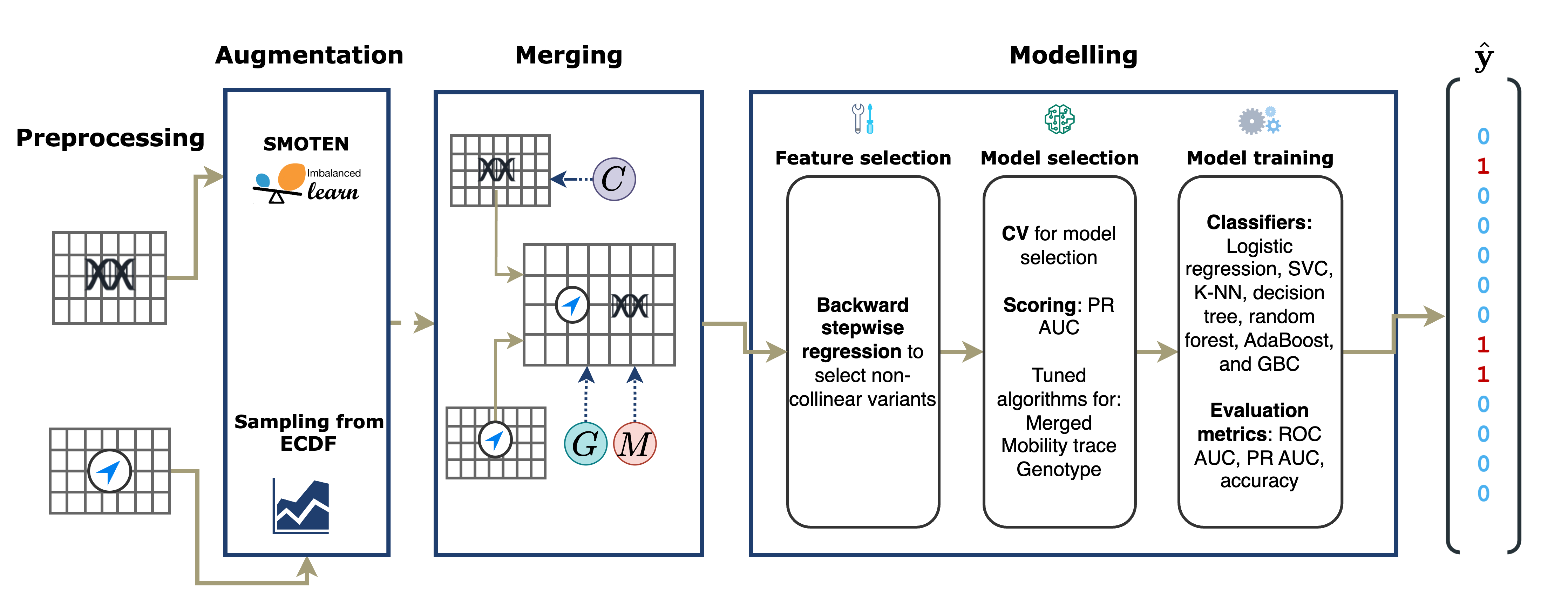
Figure 1: Overview of our integrative approach for estimating disease risk. The mobility trace and genetic data are preprocessed, then augmented to balance the genetic and mobility trace sample sizes. The augmented data is merged using a comorbidity ($C$), genetic relative risk ($G$), and mobility relative risk ($M$). In the modelling step, features and models are selected, and classifiers are trained to estimate OUD risk.

2.4 Our Approach

Recent efforts have investigated how clinical biomarkers, environmental factors, and genetic features interact to affect substance use disorders [42, 43]. In a similar manner, our framework for OUD risk prediction combines genetic and environmental modalities, but focuses on behavioral features that are extracted from mobility traces (Fig. 1). In the pre-processing and augmentation phases, we perform standard quality control measures on both the genetic and mobility data, extract features, leverage an existing data augmentation method to synthesize genetic data, and generate mobility features using a new simulation algorithm (Fig. 2). The subsequent merging phase creates hybrid (combined) observations by first sampling a case or control genetic sample at random, then sampling a case or control mobility trace based on an assumed comorbidity; ultimately, case status is assigned to the hybrid samples using relative risk parameters. The resulting samples from the pre-processing, augmentation, and merging phases enable the creation of datasets with three distinct feature sets: genetic data only, mobility traces only, and combined. In the final modelling phase we perform feature selection on the genetic data followed by model selection using cross-validation (CV) and average precision; lastly, we train a diverse set of classifiers, evaluating generalization performance through classification accuracy, $F_{1}$ score, ROC AUC, and PR AUC.

3 Methods

Our method estimates OUD risk from both genetic and mobility features extracted from experimental assays and GPS or Wi-Fi data, respectively. Since mobility trace datasets concerning disease risk are currently smaller than GWAS studies on average, we also develop a data augmentation algorithm to synthesize additional mobility trace samples. Finally, there currently does not exist any dataset that includes both genetic and mobility features in the context of disease. Therefore, we sample a case or control from the larger genetic dataset uniformly at random, append an augmented mobility trace case or control sample based on a comorbidity parameter, and finally set the case or control status based on a Bernoulli random variable model.

3.1 Genetic Features

Variability in the genome is characterized by the sequences of alternative forms of genetic variants (alleles), or genotypes, typically collected by genotyping arrays [44] or DNA sequencing [45]. Let the genotype matrix $\bm{X}^{g}$ and label vector $\bm{y}^{g}$ be $\bm{X}^{g}=(x_{ij}^{g})_{i=1,j=1}^{i=N_{g},j=L_{g}}$ and $\bm{y}^{g}=(y_{i}^{g})_{i=1}^{i=N_{g}}$, respectively, where $N_{g}$ is the number of genetic samples, $L_{g}$ is the number of genetic variants, $x_{ij}\in\{0,1,2\}$ denotes the count of the minor allele for sample $i$ and position $j$, and $y_{i}^{g}\in\{0,1\}$ denotes disease status, where 0 and 1 indicate control and case status, respectively. These data can be agnostic to prior GWAS, in which case $L_{g}\approx 10^{6}$, or be defined based on the variants that have prior associations with the disease of interest ($L_{g}\approx 10^{2}$).

3.2 Mobility Features

Mobility traces are temporally sequenced latitude and longitude positions extracted from the participant phones using GPS data or Wi-Fi association records. Mobility features are computed from mobility trace data. Let the mobility feature matrix and label vector be $\bm{X}^{m}=(x_{ij}^{m})_{i=1,j=1}^{i=N_{m},j=L_{m}}$ and $\bm{y}^{m}=(y_{i}^{m})_{i=1}^{i=N_{m}}$, respectively, where $N_{m}$ is the number of mobility trace samples, $L_{m}$ is the number of mobility features, $x_{ij}\in\mathbb{R}$ denotes the $j^{th}$ mobility feature value for sample $i$ and $y_{i}^{m}\in\{0,1\}$ is the disease status, where 0 and 1 indicate control and case status, respectively. We consider a total of $L_{m}=21$ features (Table 3) that have demonstrated utility for diagnosing diseases comorbid with OUD (primarily depression) [15, 33, 35, 14, 40, 46].

Mobility features can be categorized as either movement-based or location-based.

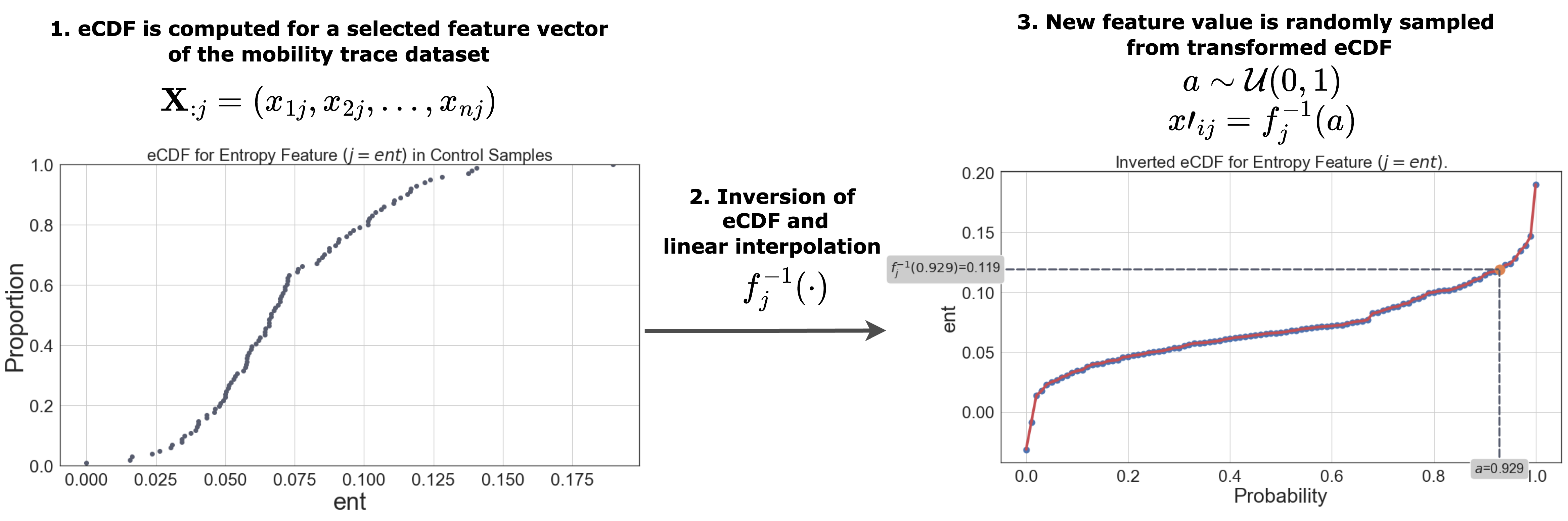
Figure 2: Mobility trace simulation. (1) From a pre-selected population (case or control), the eCDF for a feature is generated. (2) The eCDF for that feature is inverted, and linear interpolation is performed between points. (3) The simulated feature value is created by random sampling of the inverse eCDF. The process is repeated across all features and all samples in the population.

Movement-based features

Movement-based features capture the activity of an individual based on their positional trajectories. We consider $3$ movement-based features. The average moving speed in meters per second is the instantaneous speed estimated from adjacent positions. Transition time refers to the proportion of time spent in transition by sample $i$ (i.e. with moving speed $>1$ km per hour). We also compute the total distance travelled as the sum of Harversine distances between adjacent positions.

Location-based features

Location-based features represent how an individual interacts with discrete locations. First, distinct locations are identified by clustering the sample latitude and longitude positions. Then, distinct location clusters are labeled using the Google Places API, which includes bounding boxes for discrete places and $9$ categories: outdoors and recreation, professional & other places, shop & service, food, travel & transport, residence, college and university, arts & entertainment, and nightlife spots. We consider $18$ location-based features in total.

Given the empirical probability of sample $i$ being in location $k$ as $p_{ik}$, the entropy of sample $i$ is defined as $-\sum_{k}p_{ik}\log p_{ik}$ and measures the uncertainty in the location of sample $i$. Since entropy increases with the number of unique locations visited, we also compute the cluster normalized entropy,

$$\frac{-\sum_{k}p_{ik}\log p_{ik}}{\log N_{i}^{C}},$$

where $N_{i}^{C}$ is the number of clusters for sample $i$. We label the location where the sample spent the most time between the hours of $12$am to $6$am as their home. The time spent at home measures the average amount of time spent at home per day. Location variance measures the positional variability of a sample as $\log(\sigma^{2}_{lon}+\sigma^{2}_{lat})$, where $\sigma^{2}_{lon}$ and $\sigma^{2}_{lat}$ are the empirical variance of the longitude and latitude, respectively. We also consider the routine index, which quantifies the regularity of places visited over time. We compute the ratio of time spent at location $k$ in week $w$ to time spent at the same location in week $w+1$ for each location and week. The routine index is the average of these ratios across all locations and times. Additionally, we compute the average number of times a sample left or entered a location, the average time spent in each location, and the number of unique locations visited. Finally, we compute $9$ features based on the average time spent in each of the Google Places API location categories.

3.3 Generating Synthetic Mobility Feature Samples

Due to the difficulties associated with collecting mobility traces, it is often the case that $N_{m}<<N_{g}$; therefore, combining mobility and genetic data requires generating new samples of mobility traces or features. However, mobility features are typically modelled conditionally, not generatively, since they have unknown prior distributions and complex interdependencies. We address these challenges by developing a simulation algorithm that samples mobility features based on their smoothed empirical cumulative distribution functions (eCDF) (Fig. 2). We separate case mobility trace samples from controls, compute the eCDF $f_{j}(\cdot)$ of each mobility feature independently, and linearly interpolate between each observation. We generate a new mobility sample $i$ by drawing $a\sim\mathcal{U}(0,1)$ and then sampling new mobility feature $x^{\prime}_{ij}=f_{j}^{-1}(a)$ for $j=1,\dots,L_{m}$.

3.4 Hybrid Sample Simulator and Risk Models

Since there is no overlap between the genetic and mobility trace samples, we generate hybrid samples – a combination of genetic and mobility features – by considering the comorbidity $C$ between the diseases in each dataset. Comorbidity defines the co-occurrence probability of a disease with an indexed disease. Clearly, if both datasets consider the same disease, then $C=1$, but if the diseases are related yet distinct (e.g., OUD and depression) $C\leq 1$. Here, OUD is the indexed disease, and depression represents the comorbid disorder. Additionally, to model variability in disease penetrance, we make use of relative risks (RR). The RR is the probability of the outcome for one exposure group divided by the probability of the outcome of a reference exposure group [47]. For example, an RR of $10$ indicates that the exposure presents 10 times the risk of the outcome than the reference group. Comorbidity and RR enables our simulator to generate a higher diversity of realistic scenarios where both the dependence between diseases and the proportion of variance explained by genetic and environmental components can be adjusted.

Our simulator requires specification of a comorbidity $C$, genotype RR $G$, mobility trace RR $M$, and a number of samples per case and control group $n$ (Algorithms 1 and 2). While the number of samples per case and control group is less than $n$, we sample or generate a genotype vector $\hat{\bm{x}}^{g}_{i}$ uniformly at random across case and control groups. Next, we sample or generate a mobility feature vector $\hat{\bm{x}}^{m}_{i}$ from the same or different disease group according to the comorbidity $C$. Let function $\mathbbm{1}(\hat{\bm{x}}_{i})$ evaluate to $1$ if sample $\hat{\bm{x}}_{i}$ is a case and $0$ otherwise. We draw two random variables $a^{g}\sim\text{Bern}(G/(G+1))$ and $a^{m}\sim\text{Bern}(M/(M+1))$. We concatenate $\hat{\bm{x}}^{g}_{i}$ and $\hat{\bm{x}}^{m}_{i}$ to produce $\hat{\bm{x}}_{i}$ and set its disease status to $\mathbbm{1}(\hat{\bm{x}}^{g}_{i})\cdot a^{g}\lor\mathbbm{1}(\hat{\bm{x}}^{m}_{i})\cdot a^{m}$. Given $\hat{\bm{X}}=(\hat{\bm{x}}_{i})_{i=1}^{n}$, we consider $7$ models to predict OUD status: logistic regression (LOGIT), linear SVC (SVC), K-nearest neighbors (KNN), decision tree (DT), random forest (RF), AdaBoost (ADA), and gradient boosting classifiers (GBC) [48].

4 Results

For the genetic samples, we used the substance use dependence Only (SUD) and substance use dependence, childhood trauma and related disorders (SUDCT) consent groups from the Genome-Wide Association Study of Heroin Dependence ($N_{g}=2883$; study accession phs000277.v1.p1). The case samples met the Diagnostic and Statistical Manual of Mental Disorders (DSM-IV) criteria for heroin dependence (a type of opioid), and controls were individuals assessed as not meeting the DSM-IV criteria for heroin dependence along with unassessed population controls. We computed mobility features from the LifeRhythm study, which focused on the prediction of clinical depression [15, 33]; the study recorded location data every minute from University of Connecticut student participant phones over $8$ months (October 2015 to May 2016) using the LifeRhythm app. LifeRhythm runs in the background and collects three types of sensing data: GPS location data, motion-processor-generated activity data, and Wi-Fi association records that indicate when a smartphone is associated with a wireless access point. LifeRhythm study samples were associated with randomly generated identifiers and the mapping table between identifiers and real sample identities was deleted to preserve sample anonymity. Mobility features were extracted from the latitude and longitude locations of the sensing data and aggregated for each unique sample identifier, yielding $N_{m}=144$ samples. Informed consent was secured from participants in both prior studies and approval from the University of Connecticut Institutional Review Board was obtained prior to data access (reference number H20-0018) [15, 49].

4.1 Data Processing

We processed the genetic samples and variants using a combination of filters based on missingness, violations of Hardy-Weinberg equilibrium, and mismatched demographics, resulting in $N_{g}=2671$ samples [50] (see §8.1 for details). We imputed missing genomic variants and then identified SNPs that presented significant associations with OUD (EFO$\_$0010702) and opioid dependence (EFO$\_$0005611) from the NHGRI-EBI GWAS Catalog [51]. Proxy variants were identified as SNPs that were in high linkage disequilibrium with catalog variants; the resulting genotype matrix $\bm{X}^{g}$ included only the proxy variants ($L_{g}=33$). For the mobility data, we identified discrete locations in the mobility traces using the density-based spatial clustering of applications with noise (DBSCAN) algorithm tuned by 10-fold CV, labelled clusters using Google Places API, and generated the mobility feature matrix $\bm{X}^{g}$ [52]($L_{m}=21$; see §8.1 for details).

Since we observed imbalance in the case-control class across consent groups in the genetic data ($n_{cases}=2170$, $n_{controls}=501$), we oversampled controls using the synthetic minority oversampling technique for categorical variables (SMOTEN) [53]. We generated $100$ random datasets using our hybrid sample simulator with number of samples $N=2000$ ($1000$ cases and controls). We varied the comorbidity probabilities $C\in\{0.6,0.8,1.0\}$, genetic and mobility RR $(G,M)\in\{(\infty,\infty),(15,5),(15,1),(10,5),(10,1),(5,5)\}$, and feature sets, including genetic data only, mobility traces only, and combined features. We standardized features by subtracting the empirical means and dividing by the empirical standard deviations of the training data.

4.2 Model Selection and Evaluation

We selected genetic features for each comorbidity level and RR configuration in held-out datasets to remove collinear features (see §8.2). Hyperparameters were selected per disease risk score model and feature set using 10-fold CV and average precision. We evaluated each model on the $100$ datasets for each feature set, comorbidity, and RR configuration using ROC AUC, PR AUC, classification accuracy, and $F_{1}$ score assuming a $0.5$ probability threshold. We interpreted fitted models using SHapely Additive exPlanations (SHAP), which estimates the change in the expected model prediction when conditioning on feature $j$ for a specific sample [54].

4.3 Risk Score Model Analysis

First, we evaluated the risk score models across the three feature sets with comorbidity, $C=0.8$, and complete disease penetrance, $(G,M)=(\infty,\infty)$. In simpler methods that did not include interaction effects (e.g., LOGIT), the models trained on merged data outperformed models trained on either modality (Table 1). In more complicated models (e.g., boosting classifiers), models trained on the merged data were indistinguishable from the same model trained on mobility features, suggesting that mobility traces are sufficient to rank samples based on disease state probabilities. The ensemble methods had significantly higher ROC AUC across the three feature sets: GBC in merged and mobility feature sets (Welch’s two sample t-test; p-values $\leq 2.93\times 10^{-8}$) and random forests in the genotype set (Welch’s two sample t-test; p-values $\leq 2.36\times 10^{-6}$). Additionally, PR AUC and $F_{1}$ scores showed similar patterns with respect to the performance of the ensemble methods (Tables 4 and 5). Models that made linear and additive effects assumptions performed markedly worse than the models that allow for more complex interactions between features, indicating that interactions between genetic variants, mobility features, or gene-by-environment may be present; this interpretation is consistent with the literature that suggests there exists significant gene-by-environment interactions in substance use disorders [55].

Table 1: ROC AUC scores across models and feature sets.

	Dataset
Model	Merged	Mobility	Genotype
LOGIT	0.68 (2.5)	0.63 (2.7)	0.63 (2.7)
SVC	0.68 (2.5)	0.63 (2.7)	0.63 (2.7)
KNN	0.69 (2.6)	0.71 (2.6)	0.66 (3.2)
DT	0.75 (3.1)	0.75 (3.6)	0.64 (2.5)
RF	0.88 (1.7)	0.88 (1.8)	0.68 (2.9)
ADA	0.89 (1.8)	0.89 (1.9)	0.63 (2.7)
GBC	0.91 (1.5)	0.91 (1.8)	0.67 (2.8)
Mean ROC AUC and standard errors ($\times 10^{-2}$) across 100 datasets with comorbidity $C=0.8$ and relative risks $(G,M)=(\infty,\infty)$. Bold values indicate models with significantly better ROC AUC than other methods within a feature set (Welch’s two sample t-test; all p-values $\leq 2.36\times 10^{-6}$).

4.3.1 Comorbidity

Next, we considered varying the comorbidity between OUD and depression, both to model the uncertainty in comorbidity between these conditions and to explore how these approaches generalize to different diseases. The PR AUC across models largely recapitulated the previous ROC AUC results (Fig. 3). Models trained on merged and mobility feature sets had higher PR AUC, though the effect was more pronounced with higher comorbidity due to the lower noise in case-control status assignment; this more closely models the case where the mobility and genetic features are computed from the same population sample. Interestingly, the difference between PR AUC in models trained on merged versus mobility trace data is higher in the lower comorbidity ($C=0.6$), suggesting that the genetic data provides some distinguishability when the case-control assignment is noisier.

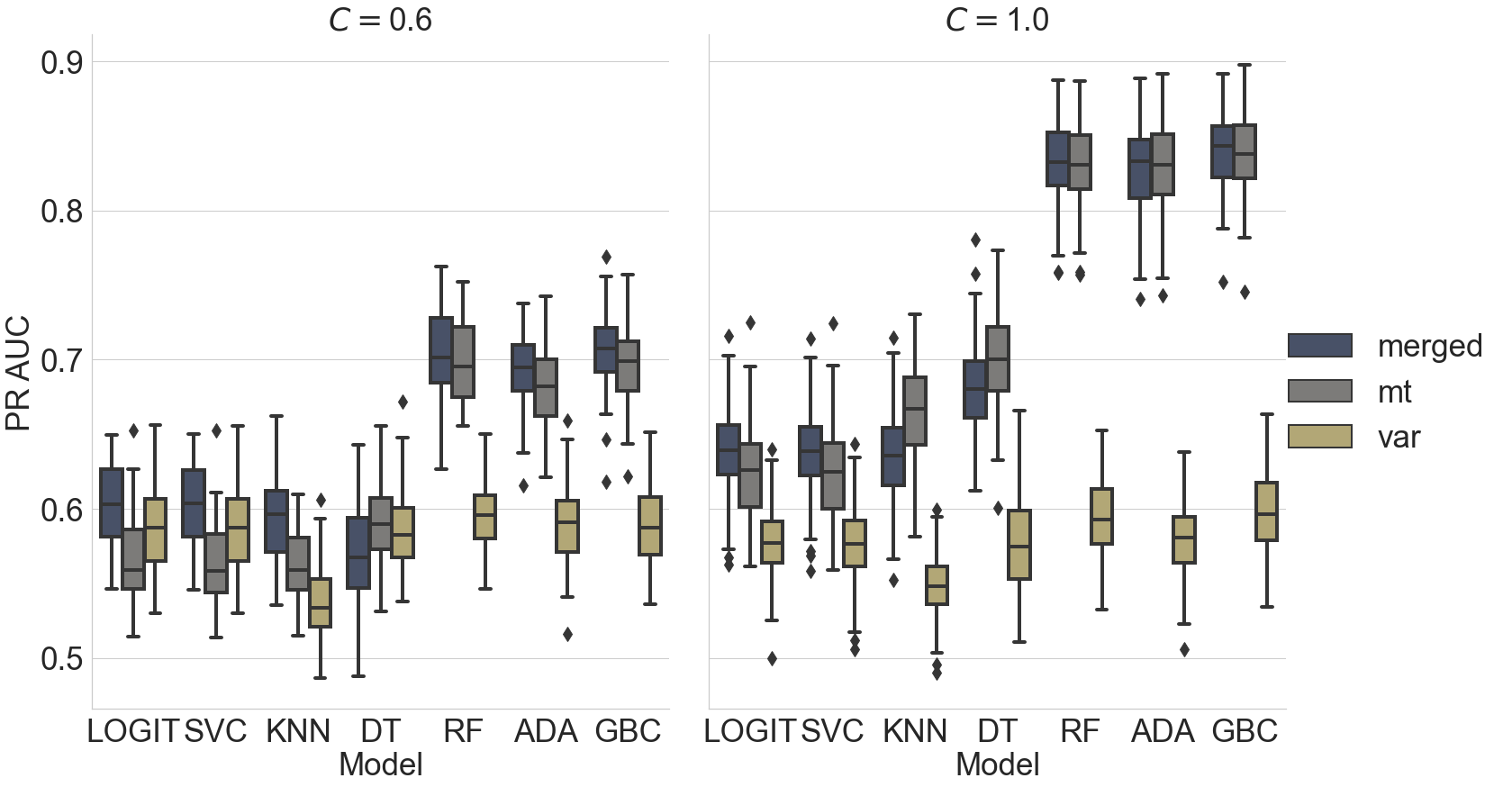
Figure 3: PR AUC across comorbidities. Box plots show the distribution PR AUC with Tukey whiskers (median $\pm$ $1.5$ $\times$ interquartile range). Each method was executed for $100$ datasets across comorbidities $C\in\{0.6,1.0\}.$ with relative risks $(G,M)=(10,5)$.

4.3.2 Relative Risk

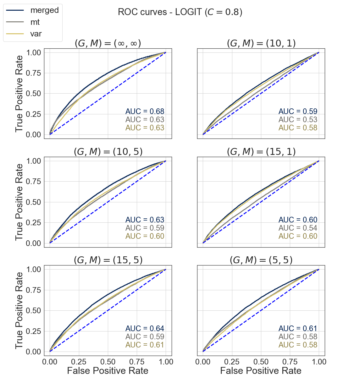
Figure 7: ROC curves across relative risk configurations for logistic regression. Logistic regression models were trained on $100$ randomly sampled datasets across relative risks $(G,M)\in\{(\infty,\infty),(10,1),(10,5),(15,1),(15,5),(5,5)\}$.

To evaluate the effect of variable disease penetrance from genetic and mobility features, we compared risk model performance across $6$ RR configurations (Tables 2 and 6). Consistent with prior results, the mean accuracy and $F_{1}$ scores show that the ensemble models have the highest performance. While increasing the RR for both genetic and mobility features increased accuracy, the relative increase was higher for mobility traces. Next, we averaged the ROC curves across the 100 randomly sampled datasets and RR configurations for a fixed $C=0.8$ and plotted the results, which include RF (Fig. 4), and logistic regression (Fig. 7) classifiers. The ROC curves also demonstrate that the largest gains in ROC AUC are achieved with higher mobility RR, but also that genotype RR distinguishes ROC curves for a fixed mobility RR. Overall, classification accuracy was diminished when compared with ROC AUC, where models performed relatively well at ranking case-control probabilities.

Table 2: Model accuracy across relative risks.

Model	($\infty$, $\infty$)	(10,1)	(10,5)	(15, 1)	(15,5)	(5,5)
LOGIT	0.63 (2.4)	0.56 (2.8)	0.59 (2.1)	0.57 (2.6)	0.60 (2.5)	0.58 (2.8)
SVC	0.63 (2.4)	0.56 (2.8)	0.59 (2.0)	0.57 (2.6)	0.60 (2.2)	0.58 (2.6)
KNN	0.62 (2.2)	0.55 (2.5)	0.59 (2.3)	0.55 (2.4)	0.59 (2.3)	0.57 (2.4)
DT	0.69 (2.9)	0.53 (2.9)	0.61 (3.2)	0.53 (2.4)	0.61 (2.7)	0.61 (2.6)
RF	0.82 (2.0)	0.59 (2.3)	0.72 (2.3)	0.61 (2.5)	0.73 (2.2)	0.70 (2.3)
ADA	0.83 (2.0)	0.59 (2.8)	0.71 (2.3)	0.60 (2.6)	0.73 (2.2)	0.69 (2.4)
GBC	0.85 (1.8)	0.59 (2.2)	0.72 (2.4)	0.60 (2.3)	0.73 (2.2)	0.70 (2.3)
Mean accuracy and standard errors ($\times 10^{-2}$) across 100 datasets and genotype and mobility RR $(G,M)$, comorbidity $C=0.8$, and combined genetic and mobility features. Bold values indicate models with significantly better accuracy than other non-bolded accuracies within a feature set (Welch’s two sample t-test; all p-values $\leq 2.9\times 10^{-2}$).

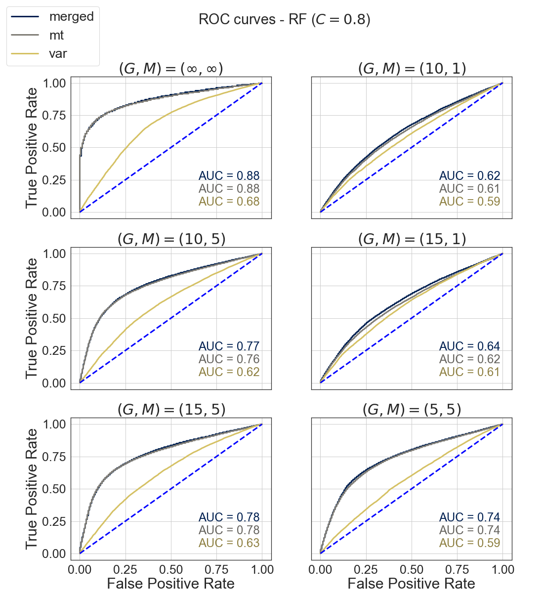
Figure 4: ROC curves across relative risk configurations. Random forest models were trained on $100$ randomly sampled datasets with comorbidity $C=0.8$ and across relative risks $(G,M)\in\{(\infty,\infty),(10,1),(10,5),(15,1),(15,5),(5,5)\}$.

4.3.3 Model Interpretation.

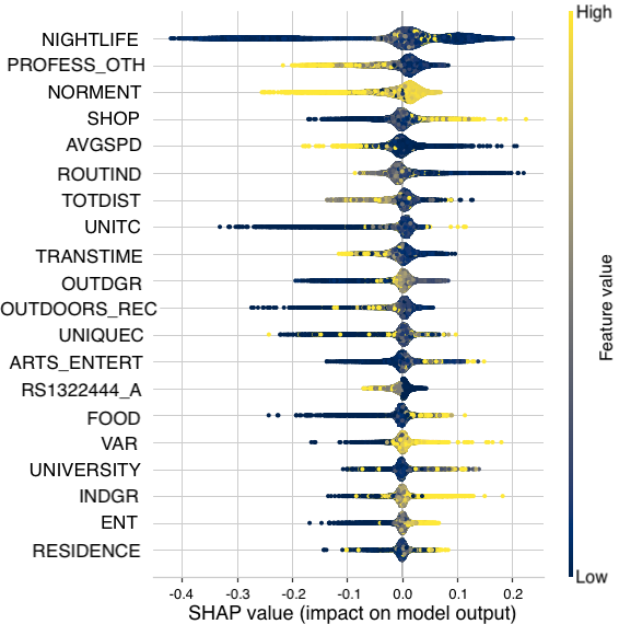
Figure 8: SHAP values across features for random forests (RF). SHAP value (x axis) and feature value (color) are shown across the $20$ features with the largest mean difference between expected and predicted values for RF. SHAP values are computed from 100 datasets with comorbidity $C=0.8$ and relative risks $(G,M)=(10,5)$.

Lastly, we investigated how features shaped model predictions using SHAP, which assigns an importance value to each feature based on its contribution to a sample prediction. We computed SHAP values for a representative ensemble (RF) and linear (SVC) model (see §8.3 for details). We observed that variants had larger mean differences between expected and predicted values (a measure of model impact) for linear SVC compared to RF (Figs. 5 and 8). In contrast, mobility features had higher SHAP value variability compared to SNPs across both models (a measure of importance).

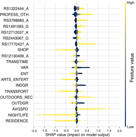
Figure 5: Feature importance vs. effects. SHAP value (x axis) and feature value (color) are shown across the $20$ features with the largest mean difference between expected and predicted values for linear SVC. SHAP values are computed from 100 datasets with comorbidity $C=0.8$ and relative risks $(G,M)=(10,5)$. SHAP values that exceeded bounds were excluded.

We also calculated the Pearson correlation coefficients ($\rho$) between SHAP and feature values, which were all significant for RF and SVC (Table 7; $\rho\neq 0$, p-values $\leq 1.8\times 10^{-3}$). Genetic variants were among the highest correlated features (in absolute value) in both RF and SVC models. Interestingly, while RF models achieved better performance, the linear SVC correlations were more consistent with prior results; for example, entropy of movement (ENT) and amount of time spent home (HOME) have been shown to be negatively and positively correlated with OUD [15] (Table 7). Location variance and time spent in shop & service (SHOP) or arts & entertainment (ARTS_ENTERT) locations also exhibited significant negative correlations with OUD. Lastly, we considered odds ratios computed from fitted logistic regression models, which indicated that exposure to genetic features show a maximum median increase of 55% in the odds of OUD (Fig. 6). In contrast, the median odds of OUD increased approximately fourfold in the two most significant mobility features (time spent in professional & other places and transition time).

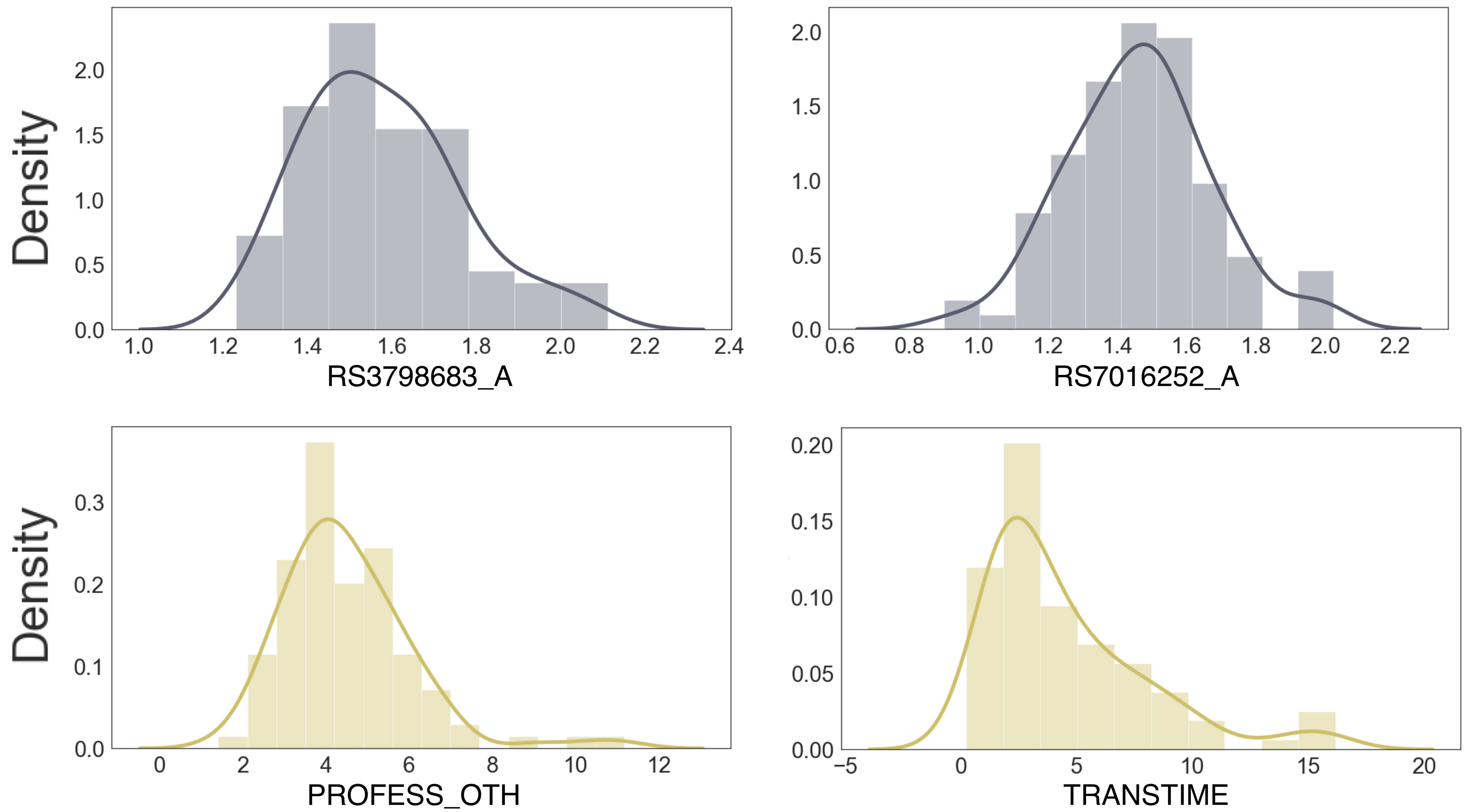
Figure 6: Odds ratios for LR models. Odds ratio densities derived from fitted LR models ordered left to right by highest median odds ratio. Each plot used 100 datasets with combined features, comorbidity $C=0.8$, and RR $(G,M)=(10,5)$.

5 Discussion

This work introduced and evaluated a strategy of risk modelling that incorporates both inherent genetic and dynamic mobility features contributing to disease risk. Our risk models are general purpose and can thus incorporate conventional features informative of OUD risk like SOAPP [17, 18]. We envision that this approach may be a useful component for clinicians to form personalized treatment strategies. There exists two mechanisms to accommodate this a priori use case: (a) if it is known that the patient requires analgesics in advance, mobility data could be generated prior to prescription; and (b) if the injury is acute, the patient could be prescribed alternative analgesics while mobility is being evaluated, though care should be taken to control for situations where the injury affects mobility. If treatment with opioids cannot be delayed, mobility traces can be used to monitor disease risk over time and inform intervention strategies due to the dynamic nature of disease risk [7].

There are several opportunities to address key limitations of our work. First, because mobility trace data does not exist for OUD, a combined genetic and mobility analysis required the fusion of datasets on different samples with related, yet distinct conditions. Collecting mobility trace and genetic data on the same population sample would address this limitation. Additionally, ensemble models achieved high performance with complete penetrance and a comorbidity of $1$ ($\approx 0.92$ PR AUC). This is likely an artifact of a small mobility trace sample size and a resulting underestimation of mobility trace population variance. Thus, increasing the size and cohort diversity of the mobility trace data should improve estimates of generalization performance. In terms of clinical support, while the risk models generally performed well with respect to ROC AUC, the ability to rank samples by class probability is less useful in clinical settings where treatment and monitoring decisions are discrete. Additionally, recent studies have shown the utility of including clinical biomarkers and other environmental factors when evaluating substance use risk [42, 43]. Future work should evaluate how these additional modalities interact with features computed from mobility traces. Finally, while genotypes are clearly causal factors for OUD, the relationship between features extracted from mobility traces and OUD is less clear. Since depression and OUD are diseases that are commonly presented together and depression status can be imputed from mobility traces with high accuracy, mobility is likely informative of OUD status; however, whether mobility is predictive of OUD risk still needs to be evaluated.

There exists many concerns that must be addressed before clinical implementation. Collecting and storing genomic and mobility data imposes risks to patients, and so disease risk modelling system using mobility traces must address security and privacy concerns. Specifically, genomic data informs disease association and forensic identification for both the patient and their relatives [56]. Spatiotemporal mobility data are highly unique and facilitate the identification of individuals using coarse and sparsely sampled data [57]. Mechanisms to mitigate privacy and security issues must be implemented both at training and inference time [58, 59]. For example, training these models requires a participating cohort to transmit their mobility data to a centralized server. However, after a model is trained, patient data can be stored locally (e.g., on their phone) which can also be used to run the trained model and transmit the prediction results to the centralized server. After models are trained or mobility features extracted, raw data can be deleted. This can be done, e.g., on a weekly basis, removing the need for long term storage of sensitive data.

Clinician decision making is vulnerable to bias, which may lead to suboptimal diagnosis and treatment outcomes [60]. Furthermore, computational modelling requires training data that may not be representative of the patient population or exhibit historical bias [61]. To identify bias, a clinical evaluation of risk supported by computational modelling should be interpretable by the doctor and explainable to both the doctor and patient. Unfortunately, machine learning techniques generally produce risk assessments that are difficult to explain based on models that are hard to interpret. Recent work in machine learning has pursued methods to explain how a machine learning algorithm arrived at a prediction (explaining a “black box”) [62], or to build machine learning models that humans can understand more easily (an interpretable “glass box”), ideally without sacrificing prediction accuracy [63, 64]. The advantages and disadvantages of models with respect to accuracy, interpretability, and explainability must be considered when using such a framework in practice.

Explainability techniques have three primary aims: (1) improve user understanding of the model; (2) communicate the uncertainty underlying a model prediction to users (domain experts or laypersons) to lead users to rely on more certain predictions; and (3) help users calibrate their trust in the model appropriately so as to maximize the joint performance of users and models [65]. Our use of SHAP exemplifies a model-agnostic feature explanation [54], however other methods exist for explaining machine learning predictions that can be evaluated within our framework, including model-specific feature importances [66, 67], counterfactual explanations, which are similar to human explanations [68, 69], and nearest-neighbors methods that identify the most similar data samples [70]. Further, we included a diversity of risk score models, in part, to evaluate performance as a function of model interpretability. Logistic regression provides odds ratios, per feature weight parameters, and uncertainty estimates, but suffered from poor performance. Conversely, while AdaBoost and GBC do not provide the same aids to interpretation or uncertainty quantification [71], they achieved significantly higher performance.

Clinical trials are necessary to evaluate the efficacy of mobility traces in disease risk estimation for OUD and depression [72]. Trials incorporating mobility data could also evaluate other disease associated risks, for example, the risk of relapse or response to treatment of those undergoing opioid agonist therapy. Since OUD is linked to opioid exposure, these trials can focus on a broader range of variants and environmental factors that increase risk of opioid exposure, like impulsivity or antisocial personality disorder [73]. Additionally, these trials will be necessary to evaluate (a) if the utility of mobility features transfer to other diseases or disorders and (b) the degree to which treatment, mobility, genetic variation, and disease status interact.

6 Conclusions

We presented the first computational approach to disease risk modelling that combines genetic features with mobility traces and applied our methods to opioid use disorder. Our pipeline extracts $21$ diverse mobility features – including $9$ newly proposed features – based on Google Places API, provides algorithms to synthesize new mobility trace samples, and simulates fused genetic and mobility trace samples using customizable comorbidity and relative risk parameters. We demonstrated that (a) combining genetic and mobility features yielded the best performing models across a variety of measures; (b) the ensemble classifiers outperformed more interpretable linear models; (c) the newly proposed features based on Google Places categories had high influence on predictions; and (d) the interactions between mobility and genetic features were consequential. Also, our approach is highly scalable as DNA sequencing and genotype array costs continue to diminish while cell phones are increasingly ubiquitous. While there exists privacy, security, bias, and generalization concerns, the development of heterogeneous risk score models may assist physicians to make more informed decisions based on disease risk estimates, which can potentially improve treatment outcomes and inform clinical or behavioral interventions.

7 Additional Methods

Table 3: Legend of mobility feature abbreviations and names.

Abbreviation	Name
VAR	Location variance
AVG SPD	Average moving speed (km/h)
ENT	Entropy
NORM ENT	Normalized entropy
HOME	Time spent at home
TRANS TIME	Transition time
TOT DIST	Total distance travelled
ROUT IND	Routine index
INDGR	Indegree
OUTDGR	Outdegree
UNIQUEC	Number of unique locations visted
UNITC	Unique cluster type
OUTDOORS_REC	‘Outdoors & Recreation’ cluster
PROFESS_OTH	‘Professional & Other Places’ cluster
SHOP	‘Shop & Service’ cluster
FOOD	‘Food’ cluster
TRANSPORT	‘Travel & Transport’ cluster
RESIDENCE	‘Residence’ cluster
UNIVERSITY	‘College & University’ cluster
ARTS_ENTERT	‘Arts & Entertainment’ cluster
NIGHTLIFE	‘Nightlife Spot’ cluster

Algorithm 1 Algorithm for generating hybrid dataset

  Inputs: Number of hybrid samples with a case status (n_cases), Number of hybrid samples with a control status (n_controls), target number of case and control samples ($n$), genotype data and labels ($\bm{X}^{g},\bm{y}^{g}$), mobility trace data and labels ($\bm{X}^{m},\bm{y}^{m}$), comorbidity $C$, mobility trace relative risk $M$, genotype relative risk $G$

  Output: hybrid_data ($\hat{\bm{X}},\hat{\bm{y}}$)

  while n_cases or n_controls $\leq$ $n$ do

     $\hat{\bm{x}}^{g}_{i}\sim s(\mathcal{U}(0,1))$ {Select case or control genotype at random}

     $\hat{\bm{x}}^{m}_{i}\leftarrow\text{simulate\_mt\_sample}^{\ast}$ according to $C$ {see Alg. 2}

     $\mathbbm{1}(\hat{\bm{x}}_{i})\leftarrow 1$ if $\bm{x}^{g}_{i}$ is a case $0$ otherwise

     $a^{g}\sim\text{Bern}(G/(G+1))$

     $a^{m}\sim\text{Bern}(M/(M+1))$

     hybrid_sample $\leftarrow$ concatenate($\hat{\bm{x}}^{g}_{i},\hat{\bm{x}}^{m}_{i}$)

     $\hat{y}\leftarrow$ $\mathbbm{1}(\hat{\bm{x}}^{g}_{i})\cdot a^{g}\lor\mathbbm{1}(\hat{\bm{x}}^{m}_{i})\cdot a^{m}$

     hyrbid_data.push(hybrid_sample, $\hat{y}$)

  end while

Algorithm 2 $\text{simulate\_mt\_sample}^{\ast}$

  Input: $\bm{X}^{m}$ {Case or control mobility samples}

  Output: synthetic_sample_output {Data point created by simulator}

  $N^{m}\leftarrow$ total number of mobility trace samples

  $L^{m}\leftarrow$ total number of mobility trace features

  for $j$ in $L^{m}$ do

     $\text{feature\_vector}\leftarrow\bm{v}_{N^{m},j}^{m}$

     $f^{-1}(\cdot)\leftarrow$ Inverted and interpolated eCDF of feature_vector

     $a\sim\mathcal{U}(0,1)$ {Random sample from uniform distribution}

     synthetic_sample_output.append($f^{-1}(a)$) {Add feature to synthetic sample}

  end for

8 Additional Results

8.1 Data Processing

8.1.1 Genetic Data Processing

We processed the genetic data using PLINK [50] by removing duplicate features and variants that (a) had minor allele frequency less than $0.01$, (b) violated Hardy-Weinberg Equilibrium ($\chi^{2}$ test; p-value less than $10^{-7}$), or (c) were missing in more than 1% of the samples. Further, samples were removed if they: had more than $1\%$ missing variants, reported sex did not match inferred sex, or identified as having a relative in the data. Missing alleles were then imputed by their mode. Because most of the GWAS catalog reference variants could not be extracted from the heroin dependence genotype samples, linkage disequilibrium was leveraged to identify variants that were in high linkage as the reference variants as proxies. Using the Ensembl REST API, proxy variants were retrieved from all African and European subpopulations in the 1000 Genomes project, phase 3 data (D_prime=1.0, window size=300kb, and $R^{2}=0.8$). Finally, identify proxy variants were used in PLINK to extract the genetic features from the opioid genotype dataset.

8.1.2 Mobility Trace Data Processing

For mobility trace data, we identified discrete locations visited by an individual by running the density-based clustering algorithm DBSCAN with hyperparameters selected via grid search (see §8.2). Distinct clusters were labelled using the Google Places API, which includes bounding boxes for discrete places and $9$ categories: outdoors and recreation, professional & other places, shop & service, food, travel & transport, residence, college and university, arts & entertainment, and nightlife spots. If a cluster centroid was not within the bounding box of any known place, we matched it with the bounding box closest to the cluster centroid using a K-D tree implementation. We then generated the mobility feature matrix $\bm{X}^{g}$ by computing the aforementioned mobility features ($L^{m}=21$).

8.2 Model selection

Since we observed collinearity in the genetic data that precluded fitting linear models, we selected genetic features using backward stepwise regression on a held out dataset for each comorbidity level and RR configuration. We also performed hyperparameter selection for each risk score model and the $3$ separate feature sets separately. We used 10-fold CV with an average precision scoring metric and a grid consisting of randomized search with $60$ iterations. We selected DBSCAN hyperparameters $\epsilon$, the minimum number of points to define a cluster, the distance metric, and the algorithm to compute the nearest neighbors. We set the hyperparameter ranges to be $0.002\leq\epsilon\leq 0.056$ and $3\leq$ min_pts $\leq 161$ in increments of $0.002$ and $2$, respectively, with the objective of maximizing the silhouette score. The selected hyperparameters were $\epsilon=0.054$, min_pts $=3$, the haversine metric, and ball_tree algorithm; $\epsilon$ and the sample coordinates were converted to radians to comply with scikit-learn’s haversine metric requirement of radian units.

8.3 Model Interpretation

We compute model interpretations using SHapely Additive exPlanations (SHAP), a model-agnostic, game-theoretic approach for interpreting fitted models and quantifying feature importance [54]. To connect optimal credit allocation with local explanations, SHAP computes Shapely values from coalitional game theory. The feature values of a data instance $x$ act as players in a coalition, and the prediction output $f(x)$ represents the value generated by the players. Shapely values aim to fairly allocate the contribution of each feature $x_{j}$ to the prediction output. SHAP represents the Shapely value explanation as an additive feature attribution method, a linear model $g$, which is an interpretable approximation of the original prediction model $f$. The explanation model is defined as $g(z^{\prime})=\phi_{0}+\sum_{j=1}^{M}\phi_{j}z^{\prime}_{j}$ where $z^{\prime}\in\{0,1\}^{M}$ selects a subset of features, $M$ is the subset size, and $\phi_{j}\in\mathbb{R}$ is the feature effect attribution for a feature $j$, the Shapely values. [54].

SHAP’s main advantages include its solid theoretical foundation in game theory, fair distribution of the prediction among feature values, and contrastive explanations brought by its use of Shapely values. Moreover, SHAP connects Local Interpretable Model-agnostic Explanations (LIME) and Shapely values, has a fast implementation for tree-based models (TreeSHAP), and allows for global model interpretations (summary plots, feature dependence, feature importance, interactions, and clustering) due to its capacity for fast computation of Shapely values.

It is equally important to recognize that the disadvantages of Shapely values also apply to SHAP: mainly, Shapley values can be misinterpreted and access to data is needed to compute them for new data (save for TreeSHAP).

We used TreeSHAP to explain our tree-based models, and chose the auto algorithm parameter for the single model explainers to optimize training time. Because AdaBoost and KNN were not natively supported by shap v.0.39, we did not generate explanation results for those methods.

SHAP summary plots combine feature importance and feature effects. Each point in the plot represents a SHAP value for a specific feature and instance. The y-axis presents the features ordered according to their average contribution, and the position on the x-axis is determined by the SHAP value. The color of each point indicates the feature value.

Table 4: PR AUC scores across models and feature sets.

	Dataset
Model	Merged	Mobility	Genotype
LOGIT	0.67 (3.3)	0.64 (3.0)	0.60 (3.0)
SVC	0.67 (3.3)	0.64 (3.0)	0.60 (3.0)
KNN	0.68 (3.3)	0.71 (3.4)	0.62 (3.1)
DT	0.75 (3.6)	0.76 (3.6)	0.61 (3.1)
RF	0.91 (4.3)	0.91 (4.3)	0.65 (3.2)
ADA	0.91 (4.4)	0.91 (4.3)	0.61 (3.2)
GBC	0.93 (4.5)	0.93 (4.4)	0.64 (3.2)
Average PR AUC and standard errors ($\times 10^{-2}$) across 100 datasets with comorbidity $C=0.8$ and relative risks $(G,M)=(\infty,\infty)$. Bold values indicate models with significantly better PR AUC than other methods for a feature set (Welch’s two sample t-test; all p-values $\leq 2.39\times 10^{-8}$).

Table 5: Model $F_{1}$ scores across models and feature sets.

	Dataset
Model	Merged	Mobility	Genotype
LOGIT	0.63 (2.5)	0.58 (2.7)	0.59 (2.9)
SVC	0.63 (2.6)	0.58 (2.9)	0.58 (2.9)
KNN	0.52 (4.2)	0.62 (3.3)	0.60 (3.4)
DT	0.68 (2.9)	0.67 (4.3)	0.59 (3.3)
RF	0.80 (2.3)	0.80 (2.3)	0.66 (3.1)
ADA	0.82 (2.1)	0.82 (2.2)	0.59 (3.0)
GBC	0.84 (1.9)	0.84 (2.3)	0.63 (3.2)
Average $F_{1}$ scores and standard errors ($\times 10^{-2}$) across 100 datasets with comorbidity $C=0.8$ and relative risks $(G,M)=(\infty,\infty)$. Bold values indicate models with significantly better $F_{1}$ scores than other methods for a feature set (Welch’s two sample t-test; all p-values $\leq 3.29\times 10^{-7}$).

Table 6: Model $F_{1}$ scores across relative risks.

Model	($\infty$, $\infty$)	(10,1)	(10,5)	(15, 1)	(15,5)	(5,5)
LOGIT	0.63 (2.5)	0.54 (3.2)	0.58 (2.4)	0.56 (3.0)	0.58 (3.0)	0.57 (3.1)
SVC	0.63 (2.6)	0.54 (3.2)	0.58 (2.4)	0.55 (3.0)	0.59 (2.7)	0.57 (3.0)
KNN	0.52 (4.2)	0.49 (3.9)	0.51 (4.3)	0.50 (3.3)	0.50 (4.0)	0.50 (3.6)
DT	0.68 (2.9)	0.50 (5.8)	0.57 (4.5)	0.53 (3.1)	0.61 (3.3)	0.54 (6.9)
RF	0.80 (2.3)	0.58 (2.8)	0.70 (2.8)	0.58 (2.8)	0.71 (2.7)	0.68 (2.6)
ADA	0.82 (2.1)	0.57 (3.2)	0.70 (2.7)	0.58 (2.9)	0.71 (2.6)	0.67 (2.7)
GBC	0.84 (1.9)	0.59 (2.7)	0.71 (2.5)	0.60 (2.7)	0.72 (2.5)	0.69 (2.4)
Mean accuracy and standard errors ($\times 10^{-2}$) across 100 datasets with comorbidity $C=0.8$, genotype and mobility RR $(G,M)$, and combined genetic and mobility features. Bold values indicate models with significantly better $F_{1}$ scores than other methods for a feature set (Welch’s two sample t-test; all p-values $\leq 3.1\times 10^{-3}$).

Table 7: Pearson correlation for SHAP and feature values for random forest and SVC models.

Model	Random Forest	Support Vector Classifier
VAR	0.5*	-0.88*
AVG SPD	-0.17*	0.86*
ENT	0.45*	-0.79*
NORM ENT	0.17*	-0.61*
HOME	-0.16*	0.59*
TRANS TIME	-0.50*	0.80*
TOT DIST	0.54*	0.62*
ROUT IND	-0.15*	-0.14*
INDGR	0.29*	-0.75*
OUTDGR	0.24*	0.59*
UNIQUEC	0.05*	0.54*
UNITC	0.02*	-0.09*
OUTDOORS_REC	-0.30*	0.81*
PROFESS_OTH	-0.74*	0.97*
SHOP	0.39*	-0.92*
FOOD	0.23*	-0.60*
TRANSPORT	0.15*	-0.76*
RESIDENCE	0.09*	-0.82*
UNIVERSITY	0.25*	-0.37*
ARTS_ENTERT	0.29*	-0.86*
NIGHTLIFE	0.05*	-0.70*
RS12130499_A	0.60*	-0.88*
RS12712037_A	-0.51*	0.89*
RS1491583_G	-0.68*	0.93*
RS2443067_G	-0.61*	0.91*
RS1322444_A	-0.75*	0.97*
RS3798683_A	-0.71*	0.95*
RS17770427_A	-0.72*	0.94*
RS10504659_A	-0.73*	0.94*
RS16939567_C	-0.69*	0.94*
RS1554347_G	-0.70*	0.94*
The asterisk (*) denotes a significant positive or negative correlation, which was calculated using a two-sided test with the null hypothesis generated using the exact distribution of the Pearson correlation coefficient (all p-value$\leq 2.2\times 10^{-16}$).

References

- [1] NIH National Institute on Drug Abuse, “Overdose Death Rates ,” Jan. 2020, accessed on 2022-11-27. [Online]. Available: https://nida.nih.gov/research-topics/trends-statistics/overdose-death-rates
- [2] W. Yu, J.-X. Hao, X.-J. Xu, and Z. Wiesenfeld-Hallin, “The development of morphine tolerance and dependence in rats with chronic pain,” Brain research, vol. 756, no. 1-2, pp. 141–146, 1997.
- [3] D. S. Hasin et al., “DSM-5 criteria for substance use disorders: recommendations and rationale,” American Journal of Psychiatry, vol. 170, no. 8, pp. 834–851, 2013.
- [4] K. E. Vowles et al., “Rates of opioid misuse, abuse, and addiction in chronic pain: a systematic review and data synthesis,” Pain, vol. 156, no. 4, pp. 569–576, Apr. 2015.
- [5] S. P. Stumbo, B. J. H. Yarborough, D. McCarty, C. Weisner, and C. A. Green, “Patient-reported pathways to opioid use disorders and pain-related barriers to treatment engagement,” Journal of substance abuse treatment, vol. 73, pp. 47–54, 2017.
- [6] C. Li, L. Qu, A. J. Matz, P. A. Murphy, Y. Liu, A. W. Manichaikul, D. Aguiar, S. S. Rich, D. M. Herrington, D. Vu et al., “Atherospectrum reveals novel macrophage foam cell gene signatures associated with atherosclerotic cardiovascular disease risk,” Circulation, vol. 145, no. 3, pp. 206–218, 2022.
- [7] A. Giannoula, A. Gutierrez-Sacristán, Á. Bravo, F. Sanz, and L. I. Furlong, “Identifying temporal patterns in patient disease trajectories using dynamic time warping: A population-based study,” Scientific reports, vol. 8, no. 1, pp. 1–14, 2018.
- [8] S. W. Choi, T. S.-H. Mak, and P. F. O’Reilly, “Tutorial: a guide to performing polygenic risk score analyses,” Nature protocols, vol. 15, no. 9, pp. 2759–2772, 2020.
- [9] N. Mavaddat et al., “Polygenic risk scores for prediction of breast cancer and breast cancer subtypes,” The American Journal of Human Genetics, vol. 104, no. 1, pp. 21–34, 2019.
- [10] S. A. Lambert et al., “Towards clinical utility of polygenic risk scores,” Hum. Mol. Genet., vol. 28, no. R2, pp. R133–R142, 2019.
- [11] C. Iyegbe et al., “The emerging molecular architecture of schizophrenia, polygenic risk scores and the clinical implications for GxE research,” Soc Psychiatry Psychiatr Epidemiol, vol. 49, no. 2, pp. 169–182, 2014.
- [12] K. Witkiewitz et al., “Mechanisms of behavior change in substance use disorder with and without formal treatment,” Annual Review of Clinical Psychology, vol. 18, pp. 497–525, 2022.
- [13] M. Whitesell, A. Bachand, J. Peel, and M. Brown, “Familial, social, and individual factors contributing to risk for adolescent substance use,” Journal of addiction, vol. 2013, 2013.
- [14] L. Canzian and M. Musolesi, “Trajectories of depression: unobtrusive monitoring of depressive states by means of smartphone mobility traces analysis,” in UbiComp. ACM, 2015, pp. 1293–1304.
- [15] A. A. Farhan et al., “Behavior vs. introspection: refining prediction of clinical depression via smartphone sensing data,” in 2016 IEEE wireless health (WH), IEEE. IEEE, 2016, pp. 1–8.
- [16] F. Ducci and D. Goldman, “The genetic basis of addictive disorders,” Psychiatric Clinics, vol. 35, no. 2, pp. 495–519, 2012.
- [17] S. F. Butler et al., “Validation of a screener and opioid assessment measure for patients with chronic pain,” Pain, vol. 112, no. 1-2, pp. 65–75, Nov. 2004.
- [18] M. O. Martel et al., “Catastrophic thinking and increased risk for prescription opioid misuse in patients with chronic pain,” Drug Alcohol Depend., vol. 132, no. 1-2, pp. 335–341, Sep. 2013.
- [19] S. F. Butler et al., “Validation of the revised Screener and Opioid Assessment for Patients with Pain (SOAPP-R),” The Journal of Pain, vol. 9, no. 4, pp. 360–372, Apr. 2008.
- [20] D. Koyyalagunta et al., “Risk stratification of opioid misuse among patients with cancer pain using the SOAPP-SF,” Pain Medicine, vol. 14, no. 5, pp. 667–675, May 2013.
- [21] D. C. Turk, K. S. Swanson, and R. J. Gatchel, “Predicting opioid misuse by chronic pain patients: a systematic review and literature synthesis,” The Clinical Journal of Pain, vol. 24, no. 6, pp. 497–508, Aug. 2008.
- [22] W.-H. Lo-Ciganic et al., “Evaluation of Machine-Learning Algorithms for Predicting Opioid Overdose Risk Among Medicare Beneficiaries With Opioid Prescriptions,” JAMA Network Open, vol. 2, no. 3, pp. e190 968–e190 968, Mar. 2019. [Online]. Available: https://jamanetwork.com/journals/jamanetworkopen/fullarticle/2728625
- [23] S. Hassanpour et al., “Identifying substance use risk based on deep neural networks and Instagram social media data,” Neuropsychopharmacology, vol. 44, no. 3, p. 487, Feb. 2019. [Online]. Available: https://www.nature.com/articles/s41386-018-0247-x
- [24] Z. Cheng et al., “Genome-wide association study identifies a regulatory variant of rgma associated with opioid dependence in european americans,” Biological psychiatry, vol. 84, no. 10, pp. 762–770, 2018.
- [25] E. C. Nelson et al., “Evidence of CNIH3 involvement in opioid dependence,” Mol. Psychiatry, vol. 21, no. 5, pp. 608–614, May 2016.
- [26] J. Gelernter et al., “Genome-wide association study of opioid dependence: multiple associations mapped to calcium and potassium pathways,” Biological Psychiatry, vol. 76, no. 1, pp. 66–74, Jul. 2014.
- [27] D. Li et al., “Genome-wide association study of copy number variations (CNVs) with opioid dependence,” Neuropsychopharmacology, vol. 40, no. 4, pp. 1016–1026, Mar. 2015.
- [28] S. E. McCabe et al., “Does early onset of non-medical use of prescription drugs predict subsequent prescription drug abuse and dependence?” Addiction, vol. 102, no. 12, pp. 1920–1930, 2007.
- [29] M. J. Edlund et al., “Risks for opioid abuse and dependence among recipients of chronic opioid therapy: results from the troup study,” Drug Alcohol Depend., vol. 112, no. 1-2, pp. 90–98, 2010.
- [30] J. L. Montalvo-Ortiz et al., “Genomewide study of epigenetic biomarkers of opioid dependence in european-american women,” Scientific reports, vol. 9, no. 1, pp. 1–9, 2019.
- [31] B. N. Cochran et al., “Factors Predicting Development of Opioid Use Disorders among Individuals who Receive an Initial Opioid Prescription: Mathematical Modeling Using a Database of Commercially-insured Individuals,” Drug Alcohol Depend., vol. 138, pp. 202–208, May 2014. [Online]. Available: https://www.ncbi.nlm.nih.gov/pmc/articles/PMC4046908/
- [32] R. Chou, G. J. Fanciullo, P. G. Fine, J. A. Adler, J. C. Ballantyne, P. Davies, M. I. Donovan, D. A. Fishbain, K. M. Foley, J. Fudin et al., “Clinical guidelines for the use of chronic opioid therapy in chronic noncancer pain,” The Journal of Pain, vol. 10, no. 2, pp. 113–130, 2009.
- [33] C. Yue et al., “Fusing location data for depression prediction,” IEEE Trans. Big Data, 2018.
- [34] S. M. Phillips, L. Cadmus-Bertram, D. Rosenberg, M. P. Buman, and B. M. Lynch, “Wearable technology and physical activity in chronic disease: opportunities and challenges,” American journal of preventive medicine, vol. 54, no. 1, p. 144, 2018.
- [35] S. Saeb et al., “Mobile Phone Sensor Correlates of Depressive Symptom Severity in Daily-Life Behavior: An Exploratory Study,” Journal of Medical Internet Research, vol. 17, no. 7, p. e175, Jul. 2015.
- [36] A. Gruenerbl, V. Osmani, G. Bahle, J. C. Carrasco, S. Oehler, O. Mayora, C. Haring, and P. Lukowicz, “Using smart phone mobility traces for the diagnosis of depressive and manic episodes in bipolar patients,” in Proceedings of the 5th Augmented Human International Conference. ACM, 2014, p. 38.
- [37] R. Wang, F. Chen, Z. Chen, T. Li, G. Harari, S. Tignor, X. Zhou, D. Ben-Zeev, and A. T. Campbell, “Studentlife: assessing mental health, academic performance and behavioral trends of college students using smartphones,” in Proceedings of the 2014 ACM international joint conference on pervasive and ubiquitous computing. ACM, 2014, pp. 3–14.
- [38] D. Ben-Zeev, E. A. Scherer, R. Wang, H. Xie, and A. T. Campbell, “Next-Generation Psychiatric Assessment: Using Smartphone Sensors to Monitor Behavior and Mental Health,” Psychiatric rehabilitation journal, vol. 38, no. 3, pp. 218–226, Sep. 2015. [Online]. Available: https://www.ncbi.nlm.nih.gov/pmc/articles/PMC4564327/
- [39] Q. Wang and J. E. Taylor, “Patterns and Limitations of Urban Human Mobility Resilience under the Influence of Multiple Types of Natural Disaster,” PLOS ONE, vol. 11, no. 1, p. e0147299, Jan. 2016. [Online]. Available: https://dx.plos.org/10.1371/journal.pone.0147299
- [40] N. Palmius et al., “Detecting Bipolar Depression From Geographic Location Data,” IEEE transactions on bio-medical engineering, vol. 64, no. 8, pp. 1761–1771, Aug. 2017. [Online]. Available: https://www.ncbi.nlm.nih.gov/pmc/articles/PMC5947818/
- [41] R. C. Smith, C. Frank, J. C. Gardiner, L. Lamerato, and K. M. Rost, “Pilot Study of a Preliminary Criterion Standard for Prescription Opioid Misuse,” The American Journal on Addictions, vol. 19, no. 6, pp. 523–528, 2010. [Online]. Available: https://onlinelibrary.wiley.com/doi/abs/10.1111/j.1521-0391.2010.00084.x
- [42] P. B. Barr, M. N. Driver, S. I.-C. Kuo, M. Stephenson, F. Aliev, R. K. Linner, J. Marks, A. P. Anokhin, K. Bucholz, G. Chan et al., “Clinical, environmental, and genetic risk factors for substance use disorders: characterizing combined effects across multiple cohorts,” Molecular psychiatry, vol. 27, no. 11, pp. 4633–4641, 2022.
- [43] S. Kinreich, J. L. Meyers, A. Maron-Katz, C. Kamarajan, A. K. Pandey, D. B. Chorlian, J. Zhang, G. Pandey, S. Subbie-Saenz de Viteri, D. Pitti et al., “Predicting risk for alcohol use disorder using longitudinal data with multimodal biomarkers and family history: a machine learning study,” Molecular psychiatry, vol. 26, no. 4, pp. 1133–1141, 2021.
- [44] M. J. Dunning, M. L. Smith, M. E. Ritchie, and S. Tavaré, “beadarray: R classes and methods for illumina bead-based data,” Bioinformatics, vol. 23, no. 16, pp. 2183–2184, 2007.
- [45] G. D. Evrony, A. G. Hinch, and C. Luo, “Applications of single-cell dna sequencing,” Annual review of genomics and human genetics, vol. 22, p. 171, 2021.
- [46] S. Rinzivillo et al., “The purpose of motion: Learning activities from individual mobility networks,” in DSAA, IEEE. IEEE, 2014, pp. 312–318.
- [47] L.-A. McNutt, C. Wu, X. Xue, and J. P. Hafner, “Estimating the Relative Risk in Cohort Studies and Clinical Trials of Common Outcomes,” American Journal of Epidemiology, vol. 157, no. 10, pp. 940–943, May 2003, _eprint: https://academic.oup.com/aje/article-pdf/157/10/940/819150/kwg074.pdf. [Online]. Available: https://doi.org/10.1093/aje/kwg074
- [48] F. Pedregosa, G. Varoquaux, A. Gramfort, V. Michel, B. Thirion, O. Grisel, M. Blondel, P. Prettenhofer, R. Weiss, V. Dubourg, J. Vanderplas, A. Passos, D. Cournapeau, M. Brucher, M. Perrot, and E. Duchesnay, “Scikit-learn: Machine learning in Python,” Journal of Machine Learning Research, vol. 12, pp. 2825–2830, 2011.
- [49] E. Maloney, L. Degenhardt, S. Darke, R. P. Mattick, and E. Nelson, “Suicidal behaviour and associated risk factors among opioid-dependent individuals: A case–control study,” Addiction, vol. 102, no. 12, pp. 1933–1941, 2007.
- [50] S. W. Choi, T. S.-H. Mak, and P. F. O’Reilly, “Tutorial: a guide to performing polygenic risk score analyses,” Nature Protocols, vol. 15, no. 9, pp. 2759–2772, Sep. 2020. [Online]. Available: https://doi.org/10.1038/s41596-020-0353-1
- [51] E. Hastings and T. Burdett, “Gwas catalog,” GWAS catalog, 2017. [Online]. Available: https://www.ebi.ac.uk/gwas/home
- [52] H.-P. K. Martin Ester, J. Sander, and X. Xu, “A density-based algorithm for discovering clusters in large spatial databases with noise,” in Proceedings of the Second International Conference on Knowledge Discovery and Data Mining, 1996, pp. 226–231.
- [53] N. V. Chawla, K. W. Bowyer, L. O. Hall, and W. P. Kegelmeyer, “SMOTE: Synthetic minority over-sampling technique,” Journal of Artificial Intelligence Research, vol. 16, pp. 321–357, jun 2002. [Online]. Available: https://doi.org/10.1613%2Fjair.953
- [54] S. M. Lundberg and S.-I. Lee, “A unified approach to interpreting model predictions,” in Advances in Neural Information Processing Systems 30. Curran Associates, Inc., 2017, pp. 4765–4774.
- [55] J. M. Vink, “Genetics of addiction: future focus on gene environment interaction?” Journal of studies on alcohol and drugs, vol. 77, no. 5, pp. 684–687, 2016.
- [56] M. Naveed, E. Ayday, E. W. Clayton, J. Fellay, C. A. Gunter, J.-P. Hubaux, B. A. Malin, and X. Wang, “Privacy in the genomic era,” ACM Computing Surveys (CSUR), vol. 48, no. 1, pp. 1–44, 2015.
- [57] Y.-A. De Montjoye, C. A. Hidalgo, M. Verleysen, and V. D. Blondel, “Unique in the crowd: The privacy bounds of human mobility,” Scientific reports, vol. 3, no. 1, pp. 1–5, 2013.
- [58] B. Berger and H. Cho, “Emerging technologies towards enhancing privacy in genomic data sharing,” Genome biology, vol. 20, no. 1, pp. 1–3, 2019.
- [59] S. Chakraborty, K. R. Raghavan, M. P. Johnson, and M. B. Srivastava, “A framework for context-aware privacy of sensor data on mobile systems,” in Proceedings of the 14th Workshop on Mobile Computing Systems and Applications, 2013, pp. 1–6.
- [60] B. H. Bornstein and A. C. Emler, “Rationality in medical decision making: a review of the literature on doctors’ decision-making biases,” Journal of evaluation in clinical practice, vol. 7, no. 2, pp. 97–107, 2001.
- [61] N. Mehrabi, F. Morstatter, N. Saxena, K. Lerman, and A. Galstyan, “A survey on bias and fairness in machine learning,” ACM Computing Surveys (CSUR), vol. 54, no. 6, pp. 1–35, 2021.
- [62] C. Molnar, Interpretable Machine Learning: A Guide for Making Black Box Models Explainable, 2nd ed. Lulu. com, 2022. [Online]. Available: https://christophm.github.io/interpretable-ml-book/
- [63] C. Rudin, C. Chen, Z. Chen, H. Huang, L. Semenova, and C. Zhong, “Interpretable machine learning: Fundamental principles and 10 grand challenges,” arXiv preprint arXiv:2103.11251, 2021.
- [64] I. Lage, A. S. Ross, B. Kim, S. J. Gershman, and F. Doshi-Velez, “Human-in-the-loop interpretability prior,” Advances in neural information processing systems, vol. 31, 2018.
- [65] G. Bansal, T. Wu, J. Zhou, R. Fok, B. Nushi, E. Kamar, M. T. Ribeiro, and D. Weld, “Does the whole exceed its parts? the effect of ai explanations on complementary team performance,” in Proceedings of the 2021 CHI Conference on Human Factors in Computing Systems, 2021, pp. 1–16.
- [66] B. H. Menze, B. M. Kelm, R. Masuch, U. Himmelreich, P. Bachert, W. Petrich, and F. A. Hamprecht, “A comparison of random forest and its gini importance with standard chemometric methods for the feature selection and classification of spectral data,” BMC bioinformatics, vol. 10, no. 1, pp. 1–16, 2009.
- [67] A. Altmann, L. Tolosi, O. Sander, and T. Lengauer, “Permutation importance: a corrected feature importance measure,” Bioinformatics, vol. 26, no. 10, pp. 1340–1347, 2010.
- [68] R. M. Byrne, “Counterfactuals in explainable artificial intelligence (xai): Evidence from human reasoning.” in IJCAI, 2019, pp. 6276–6282.
- [69] U. Bhatt, A. Xiang, S. Sharma, A. Weller, A. Taly, Y. Jia, J. Ghosh, R. Puri, J. M. Moura, and P. Eckersley, “Explainable machine learning in deployment,” in Proceedings of the 2020 conference on fairness, accountability, and transparency, 2020, pp. 648–657.
- [70] T. Cover and P. Hart, “Nearest neighbor pattern classification,” IEEE transactions on information theory, vol. 13, no. 1, pp. 21–27, 1967.
- [71] A. Malinin, L. Prokhorenkova, and A. Ustimenko, “Uncertainty in gradient boosting via ensembles,” arXiv preprint arXiv:2006.10562, 2020.
- [72] L. M. Friedman, C. D. Furberg, D. L. DeMets, D. M. Reboussin, and C. B. Granger, Fundamentals of clinical trials. Springer, 2015.
- [73] P. Köck and M. Walter, “Personality disorder and substance use disorder–an update,” Mental Health & Prevention, vol. 12, pp. 82–89, 2018.