Actively Learning Reinforcement Learning: A Stochastic Optimal Control Approach

Abstract

In this paper we provide a framework to cope with two problems: (i) the fragility of reinforcement learning due to modeling uncertainties because of the mismatch between controlled laboratory/simulation and real-world conditions and (ii) the prohibitive computational cost of stochastic optimal control. We approach both problems by using reinforcement learning to solve the stochastic dynamic programming equation. The resulting reinforcement learning controller is safe with respect to several types of constraints and it can actively learn about the modeling uncertainties. Unlike exploration and exploitation, probing and safety are employed automatically by the controller itself, resulting real-time learning. A simulation example demonstrates the efficacy of the proposed approach.

I Introduction

The field of reinforcement learning (RL) has shown significant promise across various disciplines ranging from gaming to robotics [28]. At its core, RL tries to solve an optimal control problem through maximizing some notion of a cumulative reward. Yet, with this promise of RL algorithms, a tough challenge arises when applying learned policies to real-world applications [13]. These policies, trained in lab simulations or controlled environments, may suffer a degradation in performance or even pocess an unsafe behavior [24]. This is due to modeling mismatches and discrepancies between the training environment and real-world conditions.

On the other hand, the field of stochastic optimal control [9, ch. 25], also known as dual control [30], highlights two important consequences of applying such control: caution and probing [18]. Caution can be seen as the control actions that prevent undesirable outcomes when the system is under uncertainty. Probing, on the other hand, is the actions that result in gathering information about the system’s uncertain parameters and/or states. Both these concepts play a central role in ensuring safety while enhancing the system’s learning capabilities and state observability. However, a control with such benefits is not easy to achieve, and in general, stochastic optimal control is computationally prohibitive, except for the simplest cases. Relying on dynamic programming to solve such high dimensional problems is unreasonable [4], due to the curse of dimensionality. In general, previous research has focused on suboptimal approaches [19], which are mostly application specific. In this work however, we focus on establishing a more general, less suboptimal framework.

The challenges faced by both RL and stochastic optimal control hinder their potential. Here we consider if each can serve as a solution to the other’s challenge. First, the modeling mismatch problems inherent to RL can potentially be mitigated by the caution and probing effects of stochastic optimal control. Caution imposes restrictions on the RL agent behavior under uncertainty and modelling mismatch, acting as a safeguard against false perception. Moreover, the adaptability and continuous learning of an RL agent, to correct the modelling uncertainty, can be achieved by the means of probing. Second, RL, possibly together with neural nets [20] as function approximators, can be used to mitigate the computational burden of stochastic optimal control. These hypothesized mutual benefits serve as the motivation for the work we present here.

Early work in the RL community recognized the need for stochastic policies when the agent has restricted or distorted access to the states [15]. The randomness introduced by stochastic policies diversifies chosen actions and hence achieves “artificial probing,” in a sense analogous to persistence of excitation in control theory and system identification [22]. This random way of achieving learning, in addition to not being necessarily effective in general, can render systems unsafe and even unstable. In this paper, we employ a learning architecture that addresses the fragility of RL due to uncertainties in modeling and tries to mitigate the computational challenges associated with stochastic optimal control. Therefore, we seek a controller which, unlike those that employ stochastic policies, seeks effective probing when learning is needed, and does so cautiously: respecting safety and performance conditions. We use an extended Kalman filter (EKF) to track approximates of system’s uncertainties, and we build RL on the resulting uncertainty propagation dynamics of the filter. We use the deep deterministic policy gradient approach to RL [20], which utilizes the policy gradient theorems [29, 17]. We then deploy our approach on a problem carefully designed to reflect the nuances of stochastic control to test the effectiveness of our RL approach under uncertainties.

II Problem Formulation

Consider a class of discrete-time nonlinear systems described $\forall k\in\mathbb{N}$ by,

$$x_{k+1} =f(x_{k},u_{k})+w_{k},$$ (1a)

$$y_{k} =g(x_{k})+v_{k},$$ (1b)

where $x_{k}\in\mathbb{R}^{r_{x}}$ is the state, $u_{k}\in\mathbb{R}^{r_{u}}$ is the control input, $y_{k}\in\mathbb{R}^{r_{y}}$ is the output signal, and $w_{k}\in\mathbb{R}^{r_{x}}$, $v_{k}\in\mathbb{R}^{r_{y}}$ are exogenous disturbances. The stochastic processes, $\{v_{k}\}$ and $\{w_{k}\}$, are assumed to be independent and identically distributed (i.i.d.) with continuously differentiable densities of zero means and covariances $\Sigma_{w}$ and $\Sigma_{v}$, respectively. These sequences are independent from each other and from $x_{0}$, the initial state, which has a continuously differentiable density $\pi_{0\mid 0}$. The functions $f(\cdot,\cdot)$ and $g(\cdot)$ are well-defined and continuously differentiable with respect to their arguments.

The primary goal of this work is to construct a causal control law, i.e., a control law that is only dependent upon the data accessible up until the moment of evaluating the control action. That is, $u_{k}=u_{k}(\mathcal{Z}_{k})$, where $\mathcal{Z}_{k}=\{y_{0},\ldots,y_{k},u_{0},\ldots,u_{k-1},\pi_{0\mid 0}\}$. This law has to minimize the cost functional

$$J=\mathbb{E\,}\left\{\sum_{k=0}^{N}\gamma^{k}\ell_{k}(x_{k},u_{k})\right\},$$ (2)

while satisfying the input constraints $u_{k}\in\mathbb{U}$, and with some acceptable chance probability, $1-\epsilon$, satisfying the state constraints $x_{k}\in\mathbb{X}$, with $\epsilon\in[0,1)$. The discount factor $\gamma\in(0,1)$, and the stage costs, $\ell_{k}:\mathbb{R}^{r_{x}}\times\mathbb{R}^{r_{u}}\to\mathbb{R}$, are continuously differentiable in their second arguments. The expectation and constraint satisfaction probabilities are taken with respect to all the random variables, i.e., $x_{0}$, $w_{k}$, and $v_{k}$, for all $k$.

We make no distinction between states and parameters. Since the formulation is nonlinear, if the original system has unknown or time-varying parameters, we use the concept of state augmentation [16, p. 281]. That is, the parameters are included in the state vector and the resulting augmented system is again described by (1), which then can be used for simultaneous parameters learning and control [5].

III Background: stochastic optimal control

The vector $x_{k}$ in (1a) retains its Markovian property due to the whiteness of $\{w_{k}\}_{k}$. Moreover, the observation $y_{k}$ is conditionally independent when conditioned on $x_{k}$; $\{v_{k}\}_{k}$ in (1) is also white. These assumptions are typical in partially observable Markov decision processes [6]. Under these conditions, the state $x_{k}$ cannot be directly accessed; it can only be inferred through the observation $y_{k}$, which typically is not equal to $x_{k}$. The vector $x_{k}$ is only a state in the Markovian sense, that is

$$p(x_{k+1}\mid x_{k},x_{k-1},\ldots,x_{0},u_{k},\ldots,u_{0})=p(x_{k+1}\mid x_{k},u_{k}).$$

For a decision maker or a control designer (or the learner as in [15]), an alternative “state” is required. That is, from a practical standpoint, the minimal accessible piece of information adequate to reason about the system’s future safety and performance. Consequently, this discussion gives rise to the concept of the information state, which, at time-$k$, is the state filtered density function $\pi_{k\mid k}=p(x_{k}\mid\mathcal{Z}_{k})$ [18]. As an “informative statistic,” a term used by [27] roughly means a statistic that is sufficiently informative to enable a desired control objective. However, the information state is typically infinite dimensional, which renders its applicability infeasible, computationally. In the next subsections, we shall explain the sources of this infeasibility and provide a framework to alleviate them.

III-A Separation

Adopting the information state $\pi_{k\mid k}$, a causal controller has the form $u_{k}=u_{k}(\pi_{k\mid k})$. This formulation of the control law allows the interpretation of stochastic optimal control as comprising two distinct steps [10, ch. 25]:

• Tracking $\pi_{k\mid k}$, that is, a Bayesian filter that propagates the information state [18].

• A law that assigns a value $u_{k}$ to each information state provided by the filter, such that this law minimizes (2).

In the linear Gaussian state-space model case, the information state takes an equivalent finite dimensional characterization: the state conditional mean and covariance. If the system is unconstrained and $\ell_{k}$s are quadratic, the optimal control is indifferent to the state covariance and is only a function of the mean. This explains the separation principle in LQG control design [3, ch. 8]. This separation principle differs from that in the realm of stochastic optimal control. The latter denotes the two-step interpretation listed above.

As pointed out by [30], tracking the information state $\pi_{k\mid k}$ does not solve the problem; a convenient approximation to the Bayesian filter is typically less cumbersome than finding the stochastic optimal control. The next subsection is a brief introduction to the Bayesian filter, which is then used to construct the dynamic programming equation for the stochastic case.

III-B Bayesian Filter

The system (1) can be equivalently described by, $\forall k\in\mathbb{N}$,

$$x_{k+1} \sim p(x_{k+1}\mid x_{k},u_{k}),$$

$$y_{k} \sim p(y_{k}\mid x_{k}),$$

similar to [25] due to the whiteness of $w_{k}$ and $v_{k}$. The notation $p(\cdot)$ denotes different density functions and will be identified by its arguments.

The information state can be propagated, at least in principle, through the Bayesian filter, which consists of the following two steps:

1. Time Update:

   $$p(x_{k+1}\mid u_{k},\mathcal{Z}_{k}) =$$

   $$\hskip-28.45274pt\int{p(x_{k+1}\mid u_{k},x_{k})p(x_{k}\mid\mathcal{Z}_{k})\,\textrm{d}x_{k}}.$$ (3)

2. Measurement Update:

   $$p(x_{k+1}\mid\mathcal{Z}_{k+1}) =$$

   $$\hskip-42.67912pt\frac{p(y_{k+1}\mid x_{k+1})p(x_{k+1}\mid u_{k},\mathcal{Z}_{k})}{\int{p(y_{k+1}\mid x_{k+1})p(x_{k+1}\mid u_{k},\mathcal{Z}_{k})\,\textrm{d}x_{k+1}}}.$$ (4)

Notice that to move from the filtered density at time-$k$ to $k+1$, the values of $u_{k}$ and $y_{k+1}$ are used. In order to simplify the notation, $\pi_{k\mid k}=p(x_{k}\mid\mathcal{Z}_{k})$ and $\pi_{k+1\mid k}=p(x_{k+1}\mid u_{k},\mathcal{Z}_{k})$, define the mapping

$$\pi_{k+1\mid k+1}=T(\pi_{k\mid k},u_{k},y_{k+1}),$$ (5)

where $T$ maps $\pi_{k\mid k}$ to $\pi_{k+1\mid k}$ using $u_{k}$ in (3), then to $\pi_{k+1\mid k+1}$ using $y_{k+1}$ in (4). In the next section we seek to approximate the above two steps by the EKF, which propagates approximations of the first two moments of $\pi_{k\mid k}$ [2].

III-C Stochastic Dynamic Programming

A causal control law uses only the available information up to the moment of evaluating this law. In accordance with the principle of optimality, when making the final control decision, denoted as $u_{N-1}$, and given the available information then $\mathcal{Z}_{N-1}$, the optimal cost can be determined as follows

$$\min_{u_{N-1}\in\mathbb{\bar{U}}(\pi_{N-1\mid N-1})}\mathbb{E\,}\Big{\{} \ell_{N-1}(x_{N-1},u_{N-1})+$$

$$\hskip 19.91692pt\gamma\ell_{N}(x_{N})\mid u_{N-1},\mathcal{Z}_{N-1}\Big{\}},$$

where the expectation is with respect to $w_{N-1},\,x_{N-1}$ and $v_{N}$. The set $\mathbb{\bar{U}}(\pi_{N-1\mid N-1})$ contains the control inputs in $\mathbb{U}$ such that they result in $\mathbb{P}(x_{N}\in\mathbb{X})\geq 1-\epsilon$. Notice that the optimal cost above is solely a function of the information state $\pi_{N-1\mid N-1}$; the random vectors $v_{N}$ and $w_{N-1}$ have known densities and are marginalized over via the expectation, and $u_{N-1}$ is the decision variable of the minimization. Writing explicitly the optimal cost as a function of the information state

$$V_{N-1}(\pi_{N-1\mid N-1})=$$

$$\hskip 8.53581pt\min_{u_{N-1}}\mathbb{E\,}\left\{\ell_{N-1}(x_{N-1},u_{N-1})+\gamma\ell_{N}(x_{N})\mid u_{N-1},\mathcal{Z}_{N-1}\right\}.$$

Define $V_{N}(\pi_{N\mid N})=\mathbb{E\,}\left\{\ell_{N}(x_{N})\mid\mathcal{Z}_{N}\right\}$, then

$$V_{N-1}(\pi_{N-1\mid N-1}) =\min_{u_{N-1}}\mathbb{E\,}\Big{\{}\ell_{N-1}(x_{N-1},u_{N-1})+$$

$$\hskip-8.53581pt\gamma V_{N}(T(\pi_{N-1\mid N-1},u_{N-1},y_{N}))\Big{\}}.$$ (6)

A complete version of this derivation is outlined in [18]. This recursion holds for $k=0,1,\ldots,N-1$, going backwards from the terminal boundary condition $V_{N}(\pi_{N\mid N})$. This is the stochastic dynamic programming equation, through which, a value $u_{k}$ is assigned to each information state $\pi_{k\mid k}$.

Except for the simplest cases, solving the stochastic dynamic programming equation is computationally prohibitive, primarily because of the infinite dimensionality of the information state. In the next section, we approximate the Bayesian filter by the EKF. This is primarily due to the finite dimensional representation of the information state it offers, which also tends to be practically convenient for variety of applications. Although this approximation is of a vastly reduced dimensionality, it is still of a relatively high dimensionality for problems of interest. We alleviate the latter burden by the implementation of RL.

IV Methodology

In this section we outline the EKF algorithm, and its “wide sense” (mean and covariance) approximation of the information state. We then adapt the cost in (2) to the new approximate wide-sense information state. A few, mainly cosmetic, changes to this adapted cost are implemented to make it align with the assumptions/notation of the RL algorithm which will be outlined subsequently.

IV-A EKF

We replace the infinite dimensional information state $\pi_{k\mid k}$ by a finite dimensional approximate one, namely, the state conditional mean vector $\hat{x}_{k\mid k}$ and covariance matrix $\Sigma_{k\mid k}$.

Let

$$\hat{x}_{k\mid k} =\mathbb{E\,}\left\{x_{k}\mid\mathcal{Z}_{k}\right\},\quad\hat{x}_{k\mid k-1}=\mathbb{E\,}\left\{x_{k}\mid u_{k-1},\mathcal{Z}_{k-1}\right\},$$

$$\Sigma_{k\mid k} =\mathbb{E\,}\left\{(x_{k}-\hat{x}_{k\mid k})(x_{k}-\hat{x}_{k\mid k})^{\top}\mid\mathcal{Z}_{k}\right\},$$

$$\Sigma_{k\mid k-1} =\mathbb{E\,}\left\{(x_{k}-\hat{x}_{k\mid k-1})(x_{k}-\hat{x}_{k\mid k-1})^{\top}\mid u_{k-1},\mathcal{Z}_{k-1}\right\}.$$

The EKF, similarly to the Bayesian filter, consists of the following two major steps:

1. Measurement-update

   $$\hat{x}_{k\mid k} =\hat{x}_{k\mid k-1}+L_{k}\left(y_{k}-g(\hat{x}_{k\mid k-1})\right),$$

   $$\Sigma_{k\mid k} =\Sigma_{k\mid k-1}-L_{k}H_{k}\Sigma_{k\mid k-1}.$$

2. Time-update

   $$\hat{x}_{k+1\mid k} =f(\hat{x}_{k\mid k},u_{k}),$$

   $$\Sigma_{k+1\mid k} =F_{k}\Sigma_{k\mid k}F_{k}^{\top}+\Sigma_{w}.$$

which can be combined to write,

$$\hat{x}_{k+1\mid k+1} =f(\hat{x}_{k\mid k},u_{k})+L_{k+1}\left(y_{k+1}-g(\hat{x}_{k+1\mid k})\right),$$

$$\Sigma_{k+1\mid k+1} =\left(I-L_{k+1}H_{k+1}\right)\left(F_{k}\Sigma_{k\mid k}F_{k}^{\top}+\Sigma_{w}\right),$$

where

$$L_{k} =\Sigma_{k\mid k-1}H_{k}^{\top}\left(H_{k}\Sigma_{k\mid k-1}H_{k}^{\top}+\Sigma_{v}\right)^{-1},$$

$$F_{k} =\left.\frac{\partial f(x,u_{k})}{\partial x}\right|_{x=\hat{x}_{k\mid k}},\quad H_{k}=\left.\frac{\partial h(x)}{\partial x}\right|_{x=\hat{x}_{k\mid k-1}},$$

and $\hat{x}_{0\mid 0}$, $\Sigma_{0\mid 0}$ are the initial state $x_{0}$ mean and covariance.

In general, the above conditional means and covariances are not exact; the state conditional densities $\pi_{k\mid k}$ are non-Gaussian due to the nonlinearities. Hence, $\hat{x}_{k\mid k}$ and $\Sigma_{k\mid k}$ are merely approximations to the conditional mean and covariance of $x_{k}$[2]. Define

$$\hat{\pi}_{k+1}=\hat{T}(\hat{\pi}_{k},u_{k},y_{k+1}),$$ (7)

where $\hat{\pi}_{k}=\{\hat{x}_{k\mid k},\Sigma_{k\mid k}\}$. Here $\hat{T}$ is a surrogate approximate mapping to $T$ in (5). The mapping $\hat{T}$ applies the above steps of the EKF to $\hat{x}_{k\mid k},\Sigma_{k\mid k}$, using $u_{k}$ and $y_{k+1}$, and generates $\hat{x}_{k+1\mid k+1}$ and $\Sigma_{k+1\mid k+1}$.

IV-B Cost

The first two moments provided by the EKF are sufficient to evaluate the expectation of the finite-horizon cost function in (2), given that the $\ell_{k}$s are quadratic. If not, the $\ell_{k}$s can be replaced by their second order Taylor expansion. That is, if $\ell_{k}(x_{k},u_{k})=x_{k}^{\top}Q_{k}x_{k}+u_{k}^{\top}R_{k}u_{k}$ for $k=0,\ldots,N$, the cost (2)

$$J =\mathbb{E\,}\Bigg{\{}\sum_{k=0}^{N}x_{k}^{\top}Q_{k}x_{k}+u_{k}^{\top}R_{k}u_{k}\Bigg{\}},$$

$$=\mathbb{E\,}\Bigg{\{}\sum_{k=0}^{N}\left(\hat{x}_{k\mid k}+\tilde{x}_{k}\right)^{\top}Q_{k}\left(\hat{x}_{k\mid k}+\tilde{x}_{k}\right)+u_{k}^{\top}R_{k}u_{k}\Bigg{\}},$$

where $\tilde{x}_{k}=x_{k}-\hat{x}_{k\mid k}$, and hence, cross-terms vanish under expectation, so we have

$$J=\mathbb{E\,}\Bigg{\{}\sum_{k=0}^{N}\hat{x}_{k\mid k}^{\top}Q_{k}\hat{x}_{k\mid k}+\text{trace}(Q_{k}\Sigma_{k\mid k})+u_{k}^{\top}R_{k}u_{k}\Bigg{\}},$$ (8)

since $\mathbb{E\,}\{\tilde{x}_{k}^{\top}Q_{k}\tilde{x}_{k}\}=\text{trace}(Q_{k}\Sigma_{k\mid k})$.

If the stage costs are not quadratic in $x_{k}$, we use their second order Taylor expansion. For a fixed $u_{k}\in\mathbb{U}$,

$$\ell_{k}(x_{k},u_{k}) \approx\ell_{k}(\hat{x}_{k\mid k},u_{k})+G_{k}(u_{k})\tilde{x}_{k}+\tilde{x}_{k}^{\top}C_{k}(u_{k})\tilde{x}_{k},$$

where

$$G_{k}(u_{k})=\left.\frac{\partial\ell_{k}(x,u_{k})}{\partial x}\right|_{x=\hat{x}_{k\mid k}},C_{k}(u_{k})=\left.\frac{\partial^{2}\ell_{k}(x,u_{k})}{\partial x^{2}}\right|_{x=\hat{x}_{k\mid k}}.$$

Substituting back in (2) yields the approximate cost function

$$\hat{J}(\pi_{0\mid 0}) =\mathbb{E\,}\Bigg{\{}\sum_{k=0}^{N}\ell_{k}\left(\hat{x}_{k\mid k},u_{k}\right)+\text{trace}\left(C_{k}(u_{k}\right)\Sigma_{k\mid k})\Bigg{\}}.$$ (9)

The linear term of the expansion vanishes, it is affine in $\tilde{x}_{k}$ which has zero mean.

IV-C Constraints for Safety

Two types of constraints can be considered: probabilistic constraints of polyhedral sets and probabilistic constraints of sets described by grids. The latter can handle more complicated geometries. Each type is handled and implied separately from the other, and only separate, not joint, probabilistic guarantees are provided.

IV-C1 Polyhedral Constraints

Given the following state constraint set

$$\mathbb{X}=\{x_{k}\in\mathbb{R}^{r_{x}}|Tx_{k}\leq\bar{x}\},\,\bar{x}\in\mathbb{R}^{t},$$ (10)

where $T\in\mathbb{R}^{t\times r_{x}}$ have full row rank. The cost function (2) is to be minimized subject to $u_{k}\in\mathbb{U}$ for $k=0,\ldots,N-1$, and to the probabilistic constraints

$$\mathbb{P}(x_{k}\in\mathbb{X}\mid\mathcal{Z}_{k})\geq 1-\epsilon,$$ (11)

for all $k=1,\ldots,N$. The probability measure $\mathbb{P}(\cdot\mid\mathcal{Z}_{k})$ corresponds to $x_{k}$ distributed according to the density $\pi_{k\mid k}=p(x_{k}\mid\mathcal{Z}_{k})$. The constant $\epsilon\in[0,1)$ is the tolerance, or the acceptable constraint violation rate.

Using the approximation of the first two moments of the state, the probabilistic constraints in (11) can be shown to be implied by deterministic linear constraints. This replacement of the probabilistic constraints with deterministic ones, with tighter constraints, forms the bases of tube-based stochastic Model Predictive Control methods [31, 8].

Lemma 1.

(Cantelli’s inequality) For a scalar random variable $\gamma$ with mean $\hat{\gamma}$ and variance $\Gamma$,

$$\mathbb{P}(\gamma-\hat{\gamma}\geq\eta)\leq\frac{\Gamma}{\Gamma+\eta^{2}},\,\eta\geq 0.$$ (12)

∎

Lemma 2.

For $j=1,\ldots,t$, let $T(j)$ be the $j^{\textit{th}}$ row of $T$ and $\bar{x}(j)$ be the $j^{\textit{th}}$ element of $\bar{x}$. The probabilistic constraints

$$\mathbb{P}\Big{(}T(j)x_{k}\leq\bar{x}(j)\mid\mathcal{Z}_{k}\Big{)}\leq 1-\frac{\epsilon}{t},$$ (13)

are implied by

$$T(j)\hat{x}_{k\mid k}\leq\bar{x}(j)-\sqrt{\frac{t-\epsilon}{\epsilon}}\sqrt{T(j)\Sigma_{k\mid k}T(j)^{\top}}.$$ (14)

Proof.

This result is analogous to that in [11], only the probability measure is replaced by a conditional one. ∎

Lemma 3.

Let $(\Omega,\mathcal{B},\mathbb{P})$ be a probability space and $E_{i}\in\mathcal{B}$ for $i=1,\ldots,n$. If $\mathbb{P}(E_{i})\geq 1-\epsilon/n$, for all $i=1,\ldots,n$, then $\mathbb{P}(\bigcap_{i=1}^{n}E_{i})\geq 1-\epsilon$. ∎

Proposition 1.

The following deterministic polyhedral constraints

$$T\hat{x}_{k\mid k}\leq\bar{x}-\sqrt{\frac{t-\epsilon}{\epsilon}}\sqrt{\mathrm{diag}(T\Sigma_{k\mid k}T^{\top})},$$ (15)

imply the probabilistic constraints in (10), where: $t$ is the number of rows of $T$, the square root is defined element-wise, and the function $\textrm{diag}(\cdot)$ maps a matrix to its diagonal terms.

Proof.

Notice that the state constraint sets in (10) can be written as intersection of sets

$$\mathbb{X} =\{x_{k}\in\mathbb{R}^{r_{x}}|Tx_{k}\leq\bar{x}_{k}\},$$

$$=\bigcap_{j=1}^{\top}\{x_{k}\in\mathbb{R}^{r_{x}}|T(j)x_{k}\leq\bar{x}_{k}(j)\},$$

since all rows are to be enforced simultaneously [21]. By Lemma 3, $\mathbb{P}(x_{k}\in\mathbb{X}_{k}\mid\mathcal{Z}_{k})\geq 1-\epsilon$ is implied by $\mathbb{P}(\{x_{k}\in\mathbb{R}^{r_{x}}|T(j)x_{k}\leq\bar{x}_{k}(j)\}\mid\mathcal{Z}_{k})\geq 1-\epsilon/t$. The latter is implied by (14) in Lemma 2. Stacking the inequalities in (14) for all of the $t$ rows of $T$, we get (15). Notice that with an increase in the number of rows $t$, the constraints become tighter and the approximation more conservative. ∎

Remark 1.

Proposition 1 is when the sets described by the rows $Tx_{k}\leq\bar{x}$ are to be satisfied jointly [14], which results in further constraints tightening in Lemma 3. If this is to be relaxed to satisfying these sets separately, condition in (15) can be replaced by the condition

$$T\hat{x}_{k\mid k}\leq\bar{x}-\sqrt{\frac{1-\epsilon}{\epsilon}}\sqrt{\mathrm{diag}(T\Sigma_{k\mid k}T^{\top})}.$$

$\square$

IV-C2 Grid-based Constraints

For state constraint sets of more complicated geometries, we use a grid of nodes representing the sets that the state is to avoid. These nodes can be generated, for instance, through rejection sampling using a uniform proposal density enveloping these sets.

Let $\Xi\subset\mathbb{R}^{r_{x}}$, a subset in the state-space, be the set to be avoided with high probability. That is,

$$\mathbb{P}(x_{k}\notin\Xi\mid\mathcal{Z}_{k})=1-\epsilon.$$ (16)

If $\mathbb{G}=\{\xi_{j},\,j=1,\ldots,L\}$ is a set of points, forming a grid in $\Xi$, we can replace the probabilistic constraint (16), by one described by the grid, by letting every point in the grid be an outlier with respect to the density $\pi_{k\mid k}$. For the purpose of identifying a point as an outlier, we apply the Mahalanobis distance [7], using the conditional mean $\hat{x}_{k\mid k}$ and covariance $\Sigma_{k\mid k}$ provided by the EKF. This distance is defined as

$$d_{k}(z)=\sqrt{(z-\hat{x}_{k\mid k})^{\top}\Sigma_{k\mid k}^{-1}(z-\hat{x}_{k\mid k})}.$$

Therefore, we replace (16) with

$$d_{k}(\xi_{j})>\delta,\,j=1,\ldots,L,$$

where $\delta>0$ can be related to an ellipsoidal confidence region about the mean $\hat{x}_{k\mid k}$, as in [12]. For example, a Mahalanobis distance of 2 for a univariate standard normal density corresponds to the two standard deviations confidence region about its mean. However, relating the Mahalanobis distance to probability is not clear. Probability is defined over sets, while Mahalanobis distance is over points. We can mitigate this problem by taking $\delta$ sufficiently large or having it as a hyper parameter to be tuned during simulation phase.

We assume the points of the grid are dense enough such that the ellipsoid defined by $x$ and $\delta$, $d_{k}(x)=\delta$, under any isometry, cannot be contained in $\Xi$ while it contains no points of the grid. In other word, this ellipsoid cannot be “squeezed” between points of the grid. Therefore, the amount of uncertainty dictates the density of sampling required to represent irregular sets. If the uncertainty is large, this ellipsoid is large, and hence, the gird can be less dense.

IV-C3 Soft Constraints

The following numbers, representing the state and input violations count, are added as a penalty, with a Langrange multiplier-like expression, to the cost function

$$\mathcal{A}_{k}^{1} =1\Big{\{}T\hat{x}_{k\mid k}>\bar{x}-\sqrt{\frac{t-\epsilon}{\epsilon}}\sqrt{\text{diag}(T\Sigma_{k\mid k}T^{\top})}\Big{\}},$$ (17)

$$\mathcal{A}_{k}^{2} =1\Big{\{}d_{k}(\xi_{j})>\delta,\,j=1,\ldots,L\Big{\}},$$

$$\hskip-8.53581pt\text{for }k=1,2,\ldots,N,$$

$$\mathcal{A}_{k}^{3} =1\Big{\{}u_{k}\in\mathbb{U}\Big{\}},$$

$$\hskip-8.53581pt\text{for }k=1,2,\ldots,N-1,$$

such that the cost becomes

$$\bar{J}(\pi_{0\mid 0},u_{0:N-1}) =\mathbb{E\,}\left\{\sum_{k=0}^{N}\gamma^{k}\bar{\ell}_{k}(x_{k},u_{k})\right\},$$ (18)

where $\bar{\ell}_{k}(x_{k},u_{k})=\ell_{k}(x_{k},u_{k})+\lambda\mathcal{A}_{k}$, $\mathcal{A}_{k}=\mathcal{A}_{k}^{1}+\mathcal{A}_{k}^{2}+\mathcal{A}_{k}^{3}$, and $\lambda$ is large positive number, acting as a Langrange multiplier.

The hard input constraint $u_{k}\in\mathbb{U}$, instead, can be enforced by limiting the control law to a specific family, for instance, using a saturated parameterized family for a rectangular $\mathbb{U}$. However, the input constraint penalty $\mathcal{A}_{k}^{3}$ can be practical for more complicated input constraint set $\mathbb{U}$.

IV-D Deterministic Policy Gradient

RL is an umbrella of algorithms that are rooted in the concept of stochastic approximation [6, 28, 24]. The main objective of these algorithms is to solve optimal control problems through simulating interactions between the controller and the environment. Among the numerous algorithms within the scope of RL, we opt for the Deterministic Policy Gradient algorithm [26], in particular, its deep neural net implementation [20]. While we find this algorithm convenient within the context of this paper—primarily due to its ability to handle continuous action spaces—our choice does not impose strong preferences on the selection of other RL algorithms.

IV-D1 Reward Signal and the Infinite Horizon Cost

The convention in RL literature is to deal with rewards, typically in infinite-horizon, rather than finite-horizon costs as in model predictive controllers. This adaptation is straight-forward, the reward signal can be defined as a negative saturated/bounded version of the stage-cost, $\bar{\ell}$. This saturation is done for two reasons. The first is to guarantee the convergence of the value function [6, ch. 7], hence, the infinite-horizon stochastic DPE as $N\to\infty$ is valid. From numerical stability perspective, to avoid exploding gradients, this will prove beneficial in the learning step of RL. The negative sign is to switch from the cost-minimization convention in optimal control to value-maximization in RL. Let

$$r(\hat{\pi}_{k},u_{k})=-\max\left\{\mathbb{E\,}\bar{\ell}(x_{k},u_{k}),M\right\},$$

where $M<\infty$. Consequently, the new form of the DPE in (6) is

$$\bar{V}_{N-1}(\hat{\pi}_{N-1}) =\max_{u_{N-1}}\Big{\{}r(\hat{\pi}_{N-1},u_{N-1})+$$

$$\hskip-8.53581pt\gamma\mathbb{E\,}\bar{V}_{N}(T(\pi_{N-1},u_{N-1},y_{N}))\Big{\}}.$$

As discussed above, by letting $N\to\infty$, $\bar{V}_{N}\to\bar{V}$, we have

$$\bar{V}(\hat{\pi}_{k}) =\max_{u_{k}}\Big{\{}r(\hat{\pi}_{k},u_{k})+\gamma\mathbb{E\,}\bar{V}(T(\pi_{k},u_{k},y_{k+1}))\Big{\}}.$$

To unify with RL notation, the state-action value function $Q$ [6],

$$Q(\hat{\pi}_{k},u_{k})=r(\hat{\pi}_{k},u_{k})+\gamma\mathbb{E\,}\left(Q(\hat{T}(\hat{\pi}_{k},u_{k},y_{k+1})\right).$$

We use a parameterized control policy $u_{k}=\mu_{\theta}(\hat{\pi}_{k})$, a neural net in this paper, and $\theta$ denotes the set of gains and biases of this net. If the total accumulated reward of this policy is

$$J_{\theta}(\hat{\pi}_{0}) =\mathbb{E\,}_{\mu_{\theta}}\Bigg{\{}\sum_{k=0}^{\infty}\gamma^{k}r(\hat{\pi}_{k},\mu_{\theta}(\hat{\pi}_{k})\Bigg{\}},$$

where $\mathbb{E\,}_{\mu_{\theta}}$ corresponds to a probability measure $\mathbb{P}_{\mu_{\theta}}$ defined over all the possible trajectories of $\hat{\pi}_{k}$s under the policy $\mu_{\theta}$.

The policy gradient theorems seek to find a description of the gradient $\nabla_{\theta}J_{\theta}$ which is convenient for computation. The Deterministic Policy Gradient Theorem of [26], adapted for the case of stochastic Dynamic Programming, provides the following identity

$$\nabla_{\theta}J_{\theta}=\mathbb{E}_{\mu_{\theta}}\Big{[}\nabla_{u}Q(\hat{\pi},u)\nabla_{\theta}\mu_{\theta}(\hat{\pi})\Big{]},$$

given the assumptions listed in Section II, $r(\hat{\pi}_{k},u_{k})$ is continuously differentiable in $u_{k}$ almost everywhere, and the Jacobian matrix $\nabla_{\theta}\mu_{\theta}(\hat{\pi})$ is continuous in $\hat{\pi}$. These conditions imply the satisfaction of Assumption A.1 in [26], almost-surely-$\mathbb{P}_{\mu_{\theta}}$.

In the deep deterministic policy gradient (DDPG) algorithm [20], $Q$ is approximated by a neural net $Q_{\psi}$ with parameters $\psi$ updated via temporal difference methods. While the above gradient is used to update the control policy neural net $\mu_{\theta}$ gains. Algorithm 1 is the DDPG algorithm adapted for the information state (instead of the state). It does not include the target networks as in [20], which can be augmented to Algorithm 1 to improve learning stability.

Algorithm 1 Actively Learning RL via DDPG

Randomly initialize the weights $\theta,\,\psi$ of the neural nets $Q_{\psi}$ and $\mu_{\theta}$;

Initialize replay buffer $\mathcal{R}$;

for $\text{episode}=1,2,\ldots$ do

     Randomly sample an initial information state $\hat{\pi}_{0}=\{\hat{x}_{0},\Sigma_{0}\}$ and a true state $x_{0}$;

     for $k=0,\ldots,N-1$ do

         Sample control actions $u_{k}=\mu_{\theta}(\hat{\pi}_{k})+\eta$ where $\eta$ is an exploration noise;

         Apply $u_{k}$ in (1a) to sample the true $x_{k+1}$;

         Using $x_{k+1}$ in (1b), sample the true $y_{k+1}$;

         Using $\hat{\pi}_{k}$, $u_{k}$ and $y_{k+1}$, evaluate $\hat{\pi}_{k+1}$ using (7);

         Calculate the reward $r(\hat{\pi}_{k},u_{k})$;

         Store the tuple $(\hat{\pi}_{k},u_{k},r(\hat{\pi}_{k},u_{k}),\hat{\pi}_{k+1})$ in $\mathcal{R}$;

         Sample a minibatch $\{(\hat{\pi}_{i},u_{i},r(\hat{\pi}_{i},u_{i}),\hat{\pi}_{i+1}),\,i=1,\ldots,M\}$ of $\mathcal{R}$;

         Set $z_{i}=r(\hat{\pi}_{i},u_{i})+\gamma Q_{\psi}(\hat{\pi}_{i+1},\mu_{\theta}(\hat{\pi}_{i+1}))$;

         Update the critic network $Q_{\psi}$ by minimizing the loss $\frac{1}{M}\sum_{i=1}^{M}\left(z_{i}-Q_{\psi}(\hat{\pi}_{i},u_{i})\right)^{2}$, w.r.t. $\psi$;

         Update the policy network $\mu_{\theta}$ using the sample average policy gradient

$$\nabla_{\theta}J_{\theta}\approx\frac{1}{M}\sum_{i=0}^{M}\nabla_{u}Q_{\psi}(\hat{\pi}_{i},u)\mid_{u=\mu_{\theta}(\hat{\pi}_{i})}\nabla_{\theta}\mu_{\theta}(\hat{\pi}_{i});$$

     end for

end for

Remark 2.

The information state $\hat{\pi}_{k}$ contains repeated elements, since $\Sigma_{k\mid k}$ is symmetric [2]. We can consider the upper triangular portion only or the diagonal elements if the cross dependencies are to be ignored. $\square$

V Numerical example

In this section we implement Algorithm 1 on a scalar state-space system with varying state observability over the state-space $\mathbb{R}$. This simple example demonstrates the behavior of the RL controller when equipped with concepts from stochastic control.

Consider this simple integrator with nonlinear measurement equation

$$x_{k+1} =x_{k}+u_{k}+w_{k},$$ (19)

$$y_{k} =\frac{1}{9}x_{k}^{3}+v_{k},$$ (20)

where $w_{k}$ and $v_{k}$ obey the assumptions listed under (1), and moreover, $w_{k}\sim\mathcal{N}(0,\Sigma_{w})$ and $w_{k}\sim\mathcal{N}(0,\Sigma_{v})$, and $\Sigma_{v}=2$, $\Sigma_{w}=2$. We start with this system since it is unstable and has varying observability.

If $x_{k}$ vanishes, $y_{k}$’s sensitivity with respect to it vanishes too. In general, the system becomes less observable as $x_{k}$ is close to the origin. Therefore, the stability of the origin and the observability of the system are important goals but in conflict. The balance we expect out of a stochastic dual controller is to drive the state close to the origin, while at the same time actively gathering information by visiting the more observable outer neighborhood.

We use a running cost $\ell(x_{k},u_{k})=x_{k}^{2}+u_{k}^{2}$, and a discount factor $\gamma=0.95$. Together, they construct the cost $J_{\theta}$ and the state-action value function $Q$. The constraints are $u_{k}\in\mathbb{U}=[-5,5]$, which we enforce by using saturated parameterized policy, rather than a Lagrangian penalty term. The latter can be the better option if $\mathbb{U}$ cannot be enforced as the range of a parameterized policy.

Deterministic policy gradient methods [26] use the actor-critic learning architecture: the actor being the control policy, and the critic is its corresponding policy evaluation in the shape of an action-value function. In this example, both networks are feedforward neural nets, with one hidden layer of size $64$. The actor network receives two inputs: the information state elements $\{\hat{x}_{k\mid k},\Sigma_{k\mid k}\}$. The output of this network is the control $u_{k}$. The critic network, approximating the action value function, takes three input values: both of the information state elements as well as the corresponding control action $u_{k}$, and it outputs $Q(\hat{\pi}_{k},u_{k})$. We use mini-batch learning, with batches of size $64$ of tuples $(\hat{\pi}_{k\mid k},u_{k},r_{k},\hat{T}(\hat{\pi}_{k},u_{k},y_{k+1}))$, and with learning rate $10^{-4}$. Figure 1 shows the convergence of the normalized accumulative reward. The normalized accumulative reward of value $1$ corresponds to $J_{\theta}=0$.

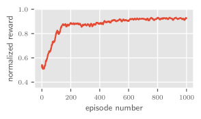
Figure 1: The average reward for the last $10$ episodes.

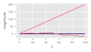
Figure 2: LQG control: The EKF information state $\hat{\pi}_{k}$: the mean $\hat{x}_{k\mid k}$ and the covariance $\Sigma_{k\mid k}$ are shown in dark blue and pink, respectively. The brown curve is the true state $x_{k}$.

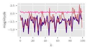
Figure 3: RL dual control: The EKF information state $\hat{\pi}_{k}$: the mean $\hat{x}_{k\mid k}$ and the covariance $\Sigma_{k\mid k}$ are shown in dark blue and pink, respectively. The brown curve is the true state $x_{k}$.

A Linear Quadratic Gaussian (LQG) control is first applied: $u_{k}=K\hat{x}_{k\mid k}$, where $\hat{x}_{k\mid k}$ is the conditional mean provided by the EKF and $K$ designed according to $Q^{LQR}=R^{LQR}=1$. The result of this LQG control is shown in Figure 2, which shows system instability and filter divergence. The state covariance is blowing up and the true state is a random walk (system is an integrator with a white noise disturbance). The concept of filter divergence is inherently qualitative, making it not only difficult to delineate the conditions causing it, but also challenging to provide a clear definition. According to [2] and [16], filter divergence is when the error covariance, $\Sigma_{k\mid k}$, of a Kalman filter (or an EKF), becomes large and therefore the filter is insensitive to new measurements. This may result in the filter’s state estimate deviating significantly from the true state of the actual system. This filter divergence seen in Figure 2 is caused mainly by the LQG controller insisting on driving the state to the origin. This issue has been handled by the RL control resulting from our approach. In Figure 3, this controller does not prioritize only driving the state estimate to the origin, but also doing so while conserving some level of observability. This balance between caution and probing is what results in the overall system stability.

VI Conclusion

The presented framework is to produce an RL agent with attributes from stochastic optimal control. These attributes equip the agent with caution: safety and probing, i.e., active online learning. This is done via using RL to solve the stochastic DPE. To track the information state, we use the EKF. If it performs poorly—that is, it is a poor approximation to the Bayesian filter—the premise, on which this control design approach is built, is then inaccurate. This issue can be mitigated by using a filter that is generally “adequate” for the problem at hand. Some alternatives include: a Gaussian sum filter [1], or the incorporation of the estimation of higher order modes into the EKF [23]. Generally, what qualifies as a “sufficient” approximation to the information state is a rather complicated question.

In addition to the choice of the Bayesian filter approximation, the design of the reward signal can produce different balances of safety and exploration/exploitation. For instance,

• Prioritizing filter stability (or its accuracy) by including the true (in simulation) estimation error or by further penalizing the state covariance term in the reward signal;

• Substituting fixed or scaled state covariance in operation;

• Tuning the state disturbance $w_{k}$ covariance $\Sigma_{w}$, or in general: the EKF design.

These are some of the questions we seek to answer in our future research.

References

- [1] D. Alspach and H. Sorenson, “Nonlinear bayesian estimation using gaussian sum approximations,” IEEE transactions on automatic control, vol. 17, no. 4, pp. 439–448, 1972.
- [2] B. D. Anderson and J. B. Moore, Optimal filtering. Courier Corporation, 2012.
- [3] K. J. Åström, Introduction to stochastic control theory. Courier Corporation, 2012.
- [4] K. J. Åström and A. Helmersson, “Dual control of an integrator with unknown gain,” Computers & Mathematics with Applications, vol. 12, no. 6, pp. 653–662, 1986.
- [5] K. J. Åström and B. Wittenmark, “Problems of identification and control,” Journal of Mathematical analysis and applications, vol. 34, no. 1, pp. 90–113, 1971.
- [6] D. Bertsekas, Dynamic programming and optimal control: Volume I. Athena scientific, 2012, vol. 1.
- [7] R. G. Brereton, “The mahalanobis distance and its relationship to principal component scores,” Journal of Chemometrics, vol. 29, no. 3, pp. 143–145, 2015.
- [8] M. Cannon, Q. Cheng, B. Kouvaritakis, and S. V. Raković, “Stochastic tube mpc with state estimation,” Automatica, vol. 48, no. 3, pp. 536–541, 2012.
- [9] A. Doucet, N. De Freitas, N. J. Gordon et al., Sequential Monte Carlo methods in practice. Springer, 2001, vol. 1, no. 2.
- [10] A. Doucet, S. Godsill, and C. Andrieu, “On sequential monte carlo sampling methods for bayesian filtering,” Statistics and computing, vol. 10, no. 3, pp. 197–208, 2000.
- [11] M. Farina, L. Giulioni, L. Magni, and R. Scattolini, “A probabilistic approach to model predictive control,” in 52nd IEEE Conference on Decision and Control. IEEE, 2013, pp. 7734–7739.
- [12] G. Gallego, C. Cuevas, R. Mohedano, and N. Garcia, “On the mahalanobis distance classification criterion for multidimensional normal distributions,” IEEE Transactions on Signal Processing, vol. 61, no. 17, pp. 4387–4396, 2013.
- [13] P. Henderson, R. Islam, P. Bachman, J. Pineau, D. Precup, and D. Meger, “Deep reinforcement learning that matters,” in Proceedings of the AAAI conference on artificial intelligence, vol. 32, no. 1, 2018.
- [14] T. Homem-de Mello and G. Bayraksan, “Monte carlo sampling-based methods for stochastic optimization,” Surveys in Operations Research and Management Science, vol. 19, no. 1, pp. 56–85, 2014.
- [15] T. Jaakkola, S. Singh, and M. Jordan, “Reinforcement learning algorithm for partially observable markov decision problems,” Advances in neural information processing systems, vol. 7, 1994.
- [16] A. H. Jazwinski, Stochastic processes and filtering theory. Courier Corporation, 2007.
- [17] S. M. Kakade, “A natural policy gradient,” Advances in neural information processing systems, vol. 14, 2001.
- [18] P. R. Kumar and P. Varaiya, Stochastic systems: Estimation, identification, and adaptive control. SIAM, 2015.
- [19] J. M. Lee and J. H. Lee, “An approximate dynamic programming based approach to dual adaptive control,” Journal of process control, vol. 19, no. 5, pp. 859–864, 2009.
- [20] T. P. Lillicrap, J. J. Hunt, A. Pritzel, N. Heess, T. Erez, Y. Tassa, D. Silver, and D. Wierstra, “Continuous control with deep reinforcement learning,” arXiv preprint arXiv:1509.02971, 2015.
- [21] J. Luedtke and S. Ahmed, “A sample approximation approach for optimization with probabilistic constraints,” SIAM Journal on Optimization, vol. 19, no. 2, pp. 674–699, 2008.
- [22] G. Marafioti, R. R. Bitmead, and M. Hovd, “Persistently exciting model predictive control,” International Journal of Adaptive Control and Signal Processing, vol. 28, no. 6, pp. 536–552, 2014.
- [23] P. Naveau, M. G. Genton, and X. Shen, “A skewed kalman filter,” Journal of multivariate Analysis, vol. 94, no. 2, pp. 382–400, 2005.
- [24] B. Recht, “A tour of reinforcement learning: The view from continuous control,” Annual Review of Control, Robotics, and Autonomous Systems, vol. 2, pp. 253–279, 2019.
- [25] T. B. Schön, A. Wills, and B. Ninness, “System identification of nonlinear state-space models,” Automatica, vol. 47, no. 1, pp. 39–49, 2011.
- [26] D. Silver, G. Lever, N. Heess, T. Degris, D. Wierstra, and M. Riedmiller, “Deterministic policy gradient algorithms,” in International conference on machine learning. Pmlr, 2014, pp. 387–395.
- [27] C. Striebel, “Sufficient statistics in the optimum control of stochastic systems,” Journal of Mathematical Analysis and Applications, vol. 12, no. 3, pp. 576–592, 1965.
- [28] R. S. Sutton and A. G. Barto, Reinforcement learning: An introduction. MIT press, 2018.
- [29] R. S. Sutton, D. McAllester, S. Singh, and Y. Mansour, “Policy gradient methods for reinforcement learning with function approximation,” Advances in neural information processing systems, vol. 12, 1999.
- [30] E. Tse, Y. Bar-Shalom, and L. Meier, “Wide-sense adaptive dual control for nonlinear stochastic systems,” IEEE Transactions on Automatic Control, vol. 18, no. 2, pp. 98–108, 1973.
- [31] J. Yan and R. R. Bitmead, “Incorporating state estimation into model predictive control and its application to network traffic control,” Automatica, vol. 41, no. 4, pp. 595–604, 2005.