Hierarchical Annotated Skeleton-Guided Tree-based Motion Planning

Abstract

We present a hierarchical tree-based motion planning strategy, HAS-RRT, guided by the workspace skeleton to solve motion planning problems in robotics and computational biology. Relying on the information about the connectivity of the workspace and the ranking of available paths in the workspace, the strategy prioritizes paths indicated by the workspace guidance to find a valid motion plan for the moving object efficiently. In instances of suboptimal guidance, the strategy adapts its reliance on the guidance by hierarchically reverting to local exploration of the planning space.

We offer an extensive comparative analysis against other tree-based planning strategies and demonstrate that HAS-RRT reliably and efficiently finds low-cost paths. In contrast to methods prone to inconsistent performance across different environments or reliance on specific parameters, HAS-RRT is robust to workspace variability.

I Introduction

Motion planning algorithms have applications in many fields, from robotics [1] to microbiology [2]. Exact motion planning is PSPACE-hard and intractable, as deterministic algorithms are exponential in the number of degrees of freedom of the robot  [3]. Attention was turned to sampling-based planners to approximate the robot’s high dimensional planning space (the configuration space, or $\mathcal{C}_{space}$). The Rapidly-exploring Random Tree (RRT) algorithm [4] was a tree-based algorithm proposed to find a valid motion plan for a movable object by sampling its configuration space.

Narrow passages in the planning space are a challenge for sampling-based algorithms. The probability of randomly discovering those narrow passages is very low, hence the necessity to find ways to guide the planning process. For example, information about the connectivity of the workspace can inform that of the robot’s configuration space. Such information can be encoded in a graph called a workspace skeleton and used to guide the exploration of the configuration space. The Dynamic Region-biased RRT [5] algorithm was a skeleton-based sampling strategy that showed that the workspace skeleton could be a reliable guide.

This work presents the Hierarchical Annotated Skeleton RRT (HAS-RRT) method to quickly find workspace-guided paths in a single-query environment. Similar to [5], HAS-RRT  uses the workspace skeleton to search for paths. However, HAS-RRT  initially relies on the connectivity of the workspace to make large steps in its exploration and only retracts to focused local exploration when necessary. Additionally, because the workspace skeleton can be annotated, the strategy can be adapted to fit different motion planning applications. When the workspace skeleton contains workspace paths that can be extended to the $\mathcal{C}_{space}$ paths, HAS-RRT exploits the guidance fully, and when the skeleton is not perfectly indicative of the motion planning solution, the method can use directional hints from such a skeleton and find a solution with additional exploration more gracefully than the other methods.

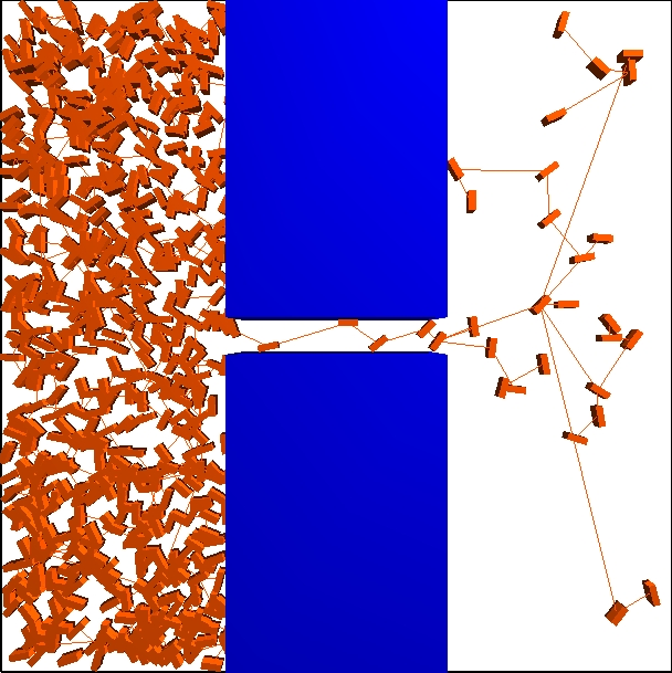
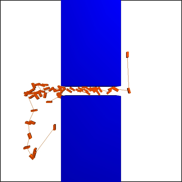
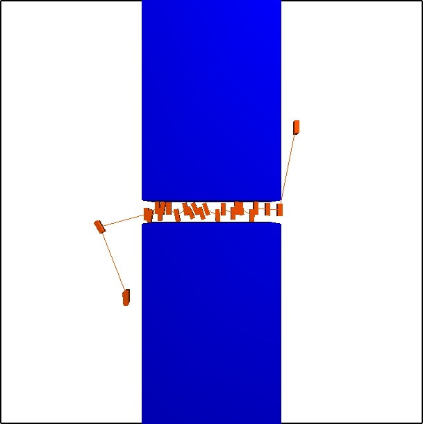
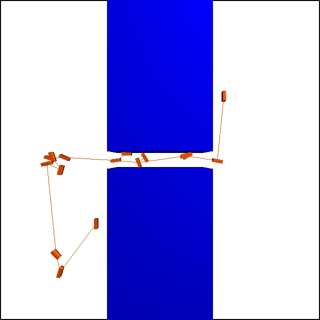
Experimental data show how the HAS-RRT method achieves improved run time, efficiency, and scalability compared to the basic RRT strategy [4], the Exploration-exploitation tree (EET) strategy [6], and the Dynamic Region RRT (DR-RRT) strategy [5]. In addition, as shown in Figure 1, HAS-RRT yields a more sparse roadmap with exploration focused on critical regions of the planning space compared to those strategies.

(a) Basic RRT [4]

(b) DR-RRT [5]

(c) EET [6]

(d) HAS-RRT

Figure 1: Roadmaps from RRT variants in a narrow passage problem. HAS-RRT  shows a better balance of exploring the open space and narrow passage.

Specifically, our contributions are:

• A novel workspace guidance for any RRT  algorithm, the Hierarchical Annotated-Skeleton guided RRT  strategy that can rapidly discover paths indicated by a workspace skeleton

• An empirical validation through robotics and computational biology experimentation that demonstrates HAS-RRT’s reliable efficiency in run time and path quality across various environments and highlights it as the best strategy for workspace-guided planning.

II Preliminaries and Previous Work

(a)

(b)

(c)

(d)

Figure 2: Example execution of Dynamic Region-biased RRT: (a) Query Skeleton (magenta) computed from a query $\{q_{s},q_{g}\}$; (b) initial region (green) placed at the source vertex of the Query Skeleton; (c) region-biased RRT growth (blue); and (d) multiple active regions (green) guiding the tree (blue) among multiple embedded arcs of the Query Skeleton (magenta) is shown.

II-A Motion Planning Preliminaries and Sampling-based Planning

A robot’s pose is described by its configuration, and the set of all possible configurations within an environment is called the configuration space, or $\mathcal{C}_{space}$. The dimension of $\mathcal{C}_{space}$ is the same as the number of degrees of freedom of the robot. $\mathcal{C}_{space}$ is partitioned into $\mathcal{C}_{free}$ (the set of valid configurations, or the free space) and $\mathcal{C}_{obst}$ (the set of invalid configurations, or the obstacle space). Given a start configuration $q_{start}$ and a goal configuration $q_{goal}$, the goal of a motion planning problem is to find a path from $q_{start}$ to $q_{goal}$ which lies entirely in $\mathcal{C}_{free}$. This is called a query.

Sampling-based planning algorithms approximate $\mathcal{C}_{space}$, since it is difficult to calculate exactly. These methods randomly generate configurations in the $\mathcal{C}_{space}$ and connect them to build a representational graph. Examples of such methods include probabilistic roadmaps (PRM) [7] and rapidly exploring random trees (RRT) [4]. In this work, we focus on RRT and some of its variations to study problems related to accessibility.

RRT algorithms are generally used to solve single-query motion planning problems. The tree starts at the start configuration, $q_{start}$. In each algorithm iteration, a random direction, $q_{rand}$, is sampled, and its nearest neighbor $q_{near}$ in the tree is identified. An extension from $q_{near}$ to $q_{rand}$ is attempted to expand the tree. After enough iterations, the tree reaches the goal, and the query is solved.

Since the direction to expand the tree is randomly selected, the RRT algorithm is probabilistically complete, meaning that if a solution exists, the probability of finding it increases as more time and resources are spent growing the tree. This, however, also implies that the algorithm struggles in more constrained environments. For example, if an environment has many dead ends, the basic RRT algorithm may waste time exploring unnecessary directions.

II-B Workspace-guided Planning

Information about the workspace is used to bias sampling towards $\mathcal{C}_{free}$ for more optimal paths or faster search time. Many methods use the workspace to guide planning, and here we describe a few.

Some methods perform a preliminary search of the workspace before sampling. The Exploration-Exploitation Trees (EET) algorithm [6] first explores the workspace by randomly growing a tree of spheres from the start position to the goal. This is called the ‘Wavefront’ expansion tree, and with it, EET grows an RRT in the $\mathcal{C}_{space}$, exploiting the pre-explored sphere regions. If exploitation fails in difficult regions, the planner gradually shifts its behavior to exploration with regular sampling-based planning. The wavefront exploration process is highly sensitive to the positioning of the start and goal configurations and the variability of region sizes in the environment. In addition, the information about the workspace is acquired by using clearance-based spheres that are randomly expanded to cover the free workspace. In environments with narrow passages, this process often takes too long.

Workspace Decomposition Strategies [8, 9, 10] steer sampling in the free workspace. For example, SyCLoP [11] uses an RRT to sample frontier decomposition regions. The decomposition of the workspace is limited as a guide, however, because it does not contain information about the topology of the workspace.

A workspace skeleton has been shown to provide better guidance for sampling. A workspace skeleton is a graph that denotes the connectivity of the workspace [12]. The vertices of the skeleton denote regions in the workspace, and the edges denote connectivity between them. A skeleton can be computed geometrically or provided by a user.

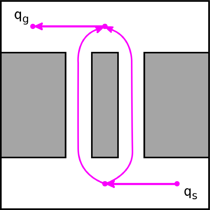
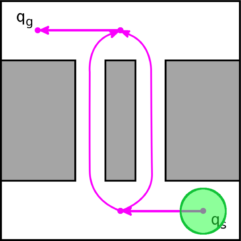
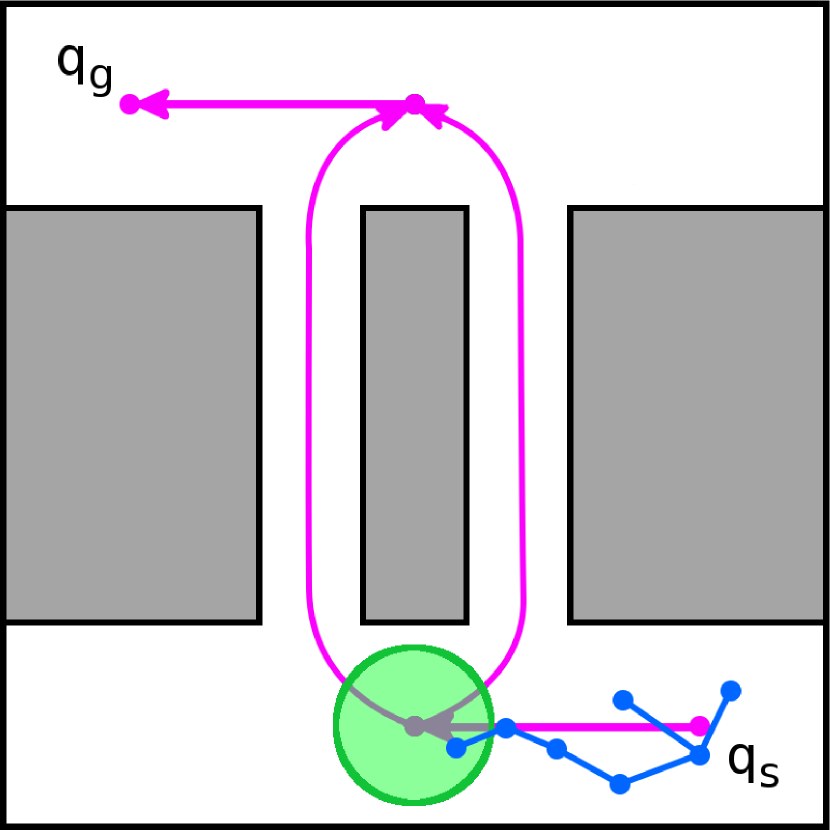
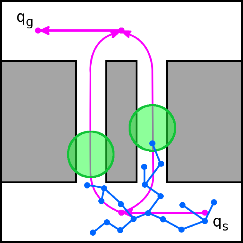
A precursor of the work presented in this paper is the Dynamic Region-biased RRT[5], detailed in Figure 2. The workspace has obstacles and a Reeb graph [13] skeleton. To speed up the process, the workspace skeleton has been pruned and directed to only have parts connecting the current start to the current goal. A sampling region is instantiated close to $q_{start}$ and expanded along the nearest skeleton edge until it reaches the next skeleton vertex and splits into several regions, one for each adjacent edge. The process ends when one of the regions is close enough to the goal to solve the query.

Dynamic Region-biased RRT  is efficient because the tree is guided through the connected free space, simplifying the narrow passage problem and preventing the tree from being stagnant. However, Dynamic Region-biased RRT  does unnecessary exploration by expanding the dynamic region in small steps along the skeleton edge.

III Method Description

(a)

(b)

(c)

(d)

(e)

(f)

(g)

(h)

Figure 3: Example execution of the Hierarchical skeleton-guided RRT: (a) Query Skeleton (purple) computed from a query $q_{s}$, $q_{g}$; (b)initial region (green) placed at the source vertex of the Query Skeleton; (c) a full extension to the end of the skeleton edge; (d) region splits into two regions at the adjacent vertices; (e) an invalid extension is attempted; (f) after a failed extension, a local expansion is attempted; (g) the weight of the failed region is adjusted to bias the tree to alternative path options; (h) the tree after a few iterations.

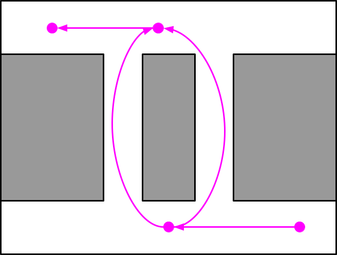
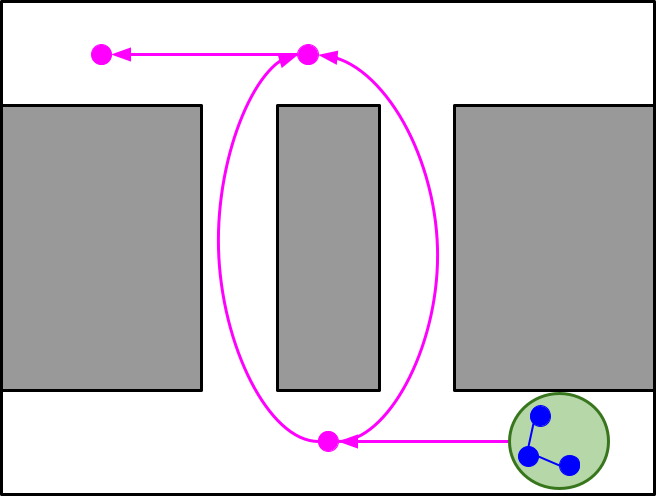
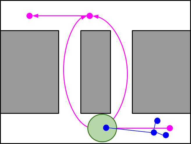
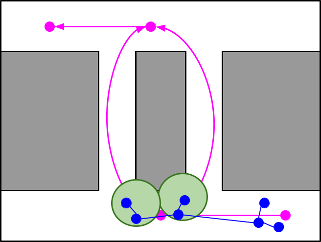
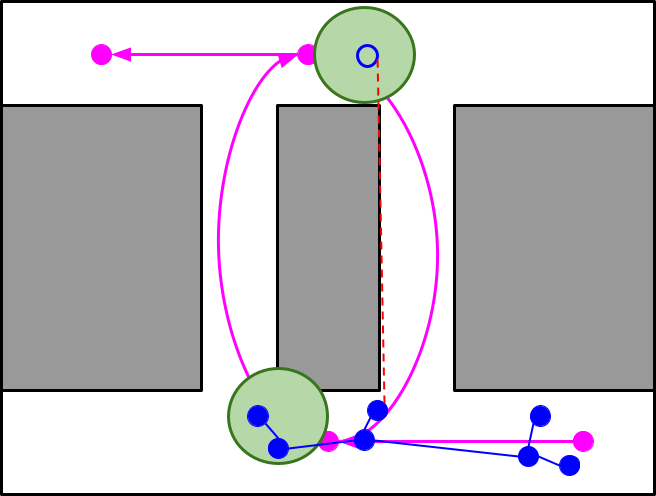
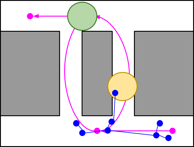
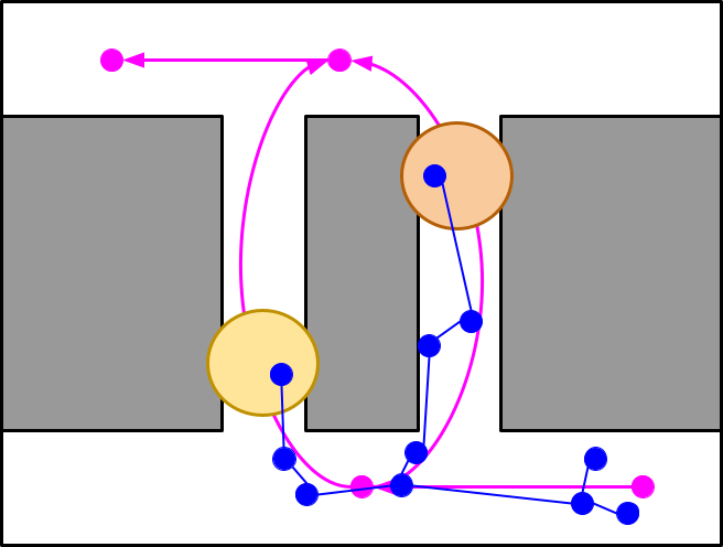
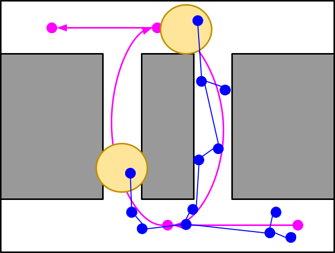
The Hierarchical Annotated-Skeleton guided RRT (HAS-RRT) algorithm (Figure 3 and Algorithm 1) improves upon the previous approach of DR-RRT by combining exploitation of the skeleton’s guidance with local exploration to better adapt to the nature of the surrounding environment. Using the connectivity mapped by the workplace skeleton, HAS-RRT aims to use longer edge extensions and smaller local extensions when the environment is denser or the skeleton is less reliable. This allows the algorithm to prioritize paths directly denoted by the skeleton and add exploration only as necessary.

The inputs to the algorithm are the environment that the robot needs to move through, the start configuration $q_{start}$, the goal configuration $q_{goal}$, and a workspace skeleton.

III-A Planning

Algorithm 1 Hierarchical Annotated Skeleton RRT

0:  Environment $env$, Start $s$, Goal $g$, Annotated Skeleton $aws$

1:  $daws\leftarrow{\tt DirectAndPruneSkeleton}(aws,s)$

2:  $tree\leftarrow s$

3:  $activeRegions\leftarrow{\tt InitializeRegion}(daws,s)$

4:  while $!{\tt PathFound}(q_{start},q_{goal})$ do

5:     $r\leftarrow{\tt SelectRegion}(activeRegions,daws)$

6:     $q_{rand}\leftarrow{\tt Sample}(r)$

7:     $q_{near}=q_{new}=NULL$

8:     ${\tt AttemptExtension}(q_{rand},tree,q_{near},q_{new})$

9:     if $q_{new}\neq NULL~{}OR~{}q_{new}\in r$ then

10:        $rDist\leftarrow{\tt AdvanceRegion}(r,daws)$

11:        $r.{\tt IncrementSuccess}()$

12:     else

13:        $rDist\leftarrow{\tt RetractRegion}(r,daws,q_{near},q_{new})$

14:        $r.{\tt IncrementFailure}()$

15:     end if

16:     $region.{\tt UpdateWeight}(rDist)$

17:  end while

First, the skeleton is directed and pruned to show only the workspace paths relevant to the given query. This directed skeleton encodes information about the direction exploration should be prioritized as shown in Figure 3(a).

Initializing the tree (Lines 2 and 3 in Algorithm 1): An active region $r$ is initialized at the skeleton vertex nearest to $q_{start}$ in the workspace. The tree is initialized with the start configuration $q_{start}$ and grown until it reaches the first region. Figure 3(b) illustrates the initial region with a tree of size 3.

Expanding the tree (Lines 5 to 16 in Algorithm 1): These steps constitute the main loop that terminates when the query is solved or the algorithm runs out of resources. First, an active region is selected, and the planner samples inside for a direction to expand the tree toward. Once a valid $q_{rand}$ is sampled, an extension attempt is performed to expand the tree (Line 9 of Algorithm 1). The successful extension adds a new vertex to the tree and pushes the region that gave $q_{rand}$ to the end of its current skeleton edge. The region’s weight is also updated by incrementing its success record to increase its chances of being selected in the next iterations. A successful direct extension to the end of a skeleton edge and its branching into two regions for each adjacent edge are shown in Figures 3(c) and 3(d).

Retracting a sampling region (Lines 12-14 in Algorithm 1): If the extension does not reach the region where $q_{rand}$ was sampled, as shown in Figure 3(e), the region is pulled back toward $q_{near}$. The current implementation pulls the region halfway between $q_{rand}$ and $q_{near}$ as shown in Algorithm 2 and Figure 3(f). In addition, the region’s weight is updated by incrementing its failure record to decrease its chances of being selected in the next iterations, as shown in Figure 3(g).

Algorithm 2 Region Retraction

0:  Region $r$, Current annotated skeleton $ask$, $q_{near}$, $q_{new}$

  $edge\leftarrow ask.{\tt GetSkeletonEdge}(r)$

2:  $currPos\leftarrow r.{\tt GetCenter}()$

  if $q_{new}\neq NULL$ then

4:     $prevPos\leftarrow q_{new}$

  else

6:     $prevPos\leftarrow q_{near}$

  end if

8:  $newPos\leftarrow{\tt GetMidPoint}(prevPos,currPos)$

  $r.center\leftarrow newPos$

10:  return  $-({\tt Distance}(newPos,currPos))$

Region Selection. The planner chooses the next region using a probability distribution based on prior extension success, the directed skeleton, and the explore/exploit bias. To maintain probabilistic completeness, the whole environment also constitutes one region in case the workspace skeleton does not cover parts of the environment that comprise the motion planning solution.

III-B Adapting to skeleton quality

Prior extension success denotes extending to a sample within a region $r$. If the skeleton is reliable, then $r$ on a skeleton vertex $v$ is centered properly in $\mathcal{C}_{free}$. Thus, the algorithm is more likely to have repeated success extending into $r$ again. The directed skeleton ensures that the algorithm continues progressing toward its goal. If a particular skeleton vertex is not accurately placed in the free workspace, the samples in the corresponding $\mathcal{C}_{space}$ may not be valid as often. Thus, the success rate in the region goes down, making the region less desirable to expand into.

Strategies guided by the workspace skeleton are affected by the quality of the skeleton. In DR-RRT  when a skeleton edge does not provide reliable guidance, the sampling region on the edge leads to repeated sampling failure, which lowers its weight and eventually pushes the algorithm to follow other directions if available or degrade to random sampling of the whole environment. With HAS-RRT  the effects of poor guidance are mitigated by two things. First, the skeleton annotations help prioritize edges that lead to the desired solution, making it less likely to encounter bad guidance. Second, when a direct extension along the skeleton edge fails, the algorithm’s retraction mechanism keeps the exploration of an alternative focused on adjusting the extension at the point of failure instead of directly reverting to random sampling. This results in faster recovery from poor guidance compared to DR-RRT.

IV Validation

(a) 2D narrow passage.

(b) Grid tunnels.

(c) Extended Z-shaped tunnels.

(d) Grid Mining, with shafts (grey) and drifts (green).

(e) 8x8 3D grid maze.

Figure 4: Tested environments

We compare HAS-RRT with three other methods: Basic RRT[4], EET[6], and DR-RRT[5]. DR-RRT and EET use workspace guidance to help with sampling. These methods were chosen due to their ability to grow an RRT with additional environmental guidance. We compare with RRT because it is a baseline method. In this section, we show that HAS-RRT returns paths with high quality in the shortest or comparable to the most competent comparison.

The results below show the robustness of HAS-RRT to all environments. In each environment, one of the other planning strategies’ performance is comparable to that of HAS-RRT  but only HAS-RRT consistently yields good solutions in less time than the others. In addition, HAS-RRT is independent of parameter tuning, an added value that makes it a good choice for a non-expert user.

IV-A Environments

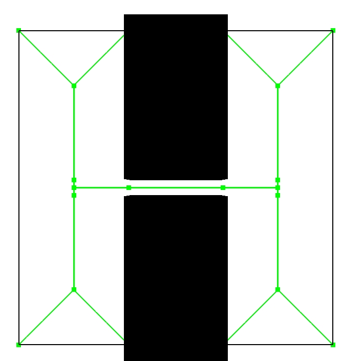
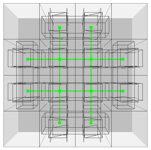
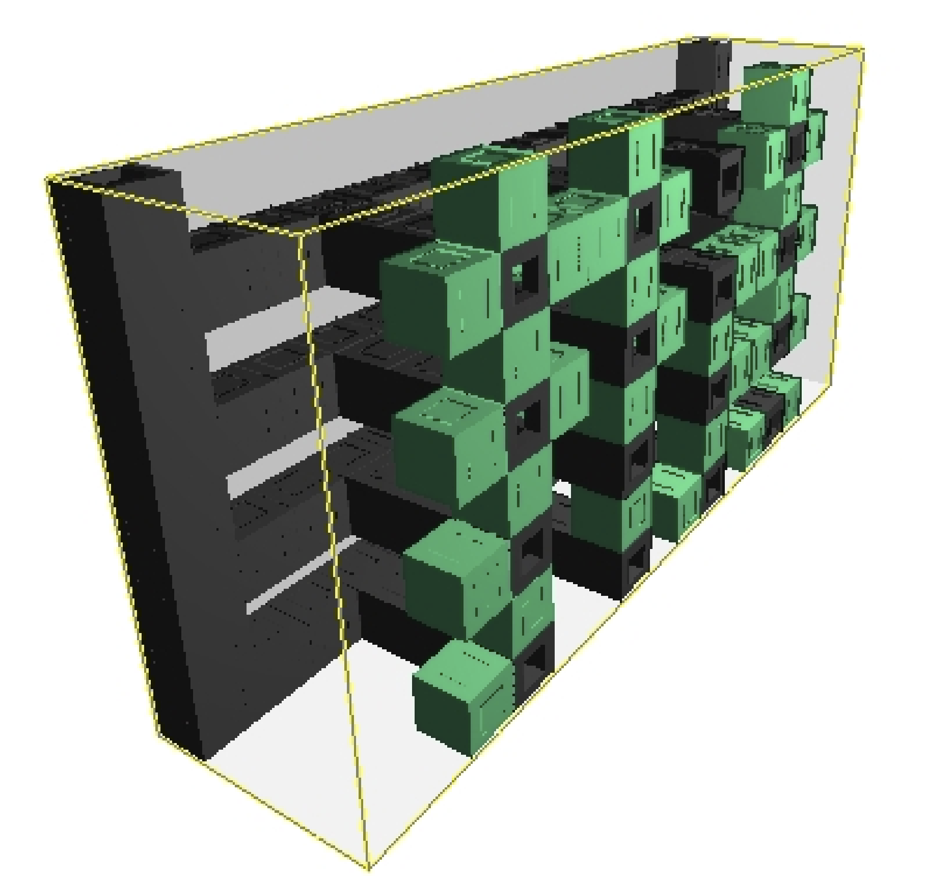
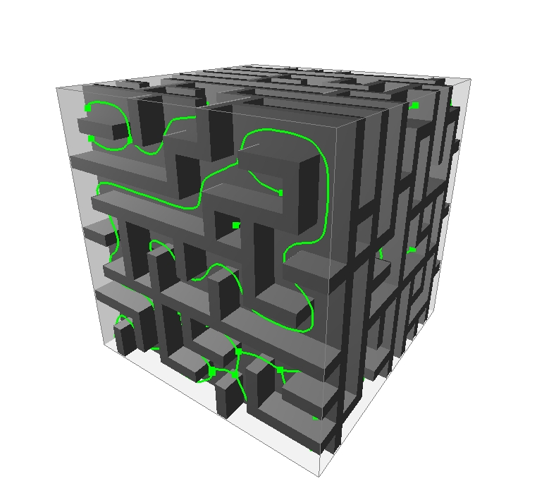
We comprehensively evaluate the method in five maze/tunnel environments shown in Figure 4. Additionally, we applied the planning strategies to a protein-ligand binding problem described in section IV-E.

1. The Simple Passage environment (Figure 4(a)) contains a narrow passage connecting the start and goal configurations from opposite corners of the environment. The skeleton shown in Figure 4(a) is a medial axis skeleton.

2. The Grid Tunnels environment (Figure 4(b)) shows a flat grid of tunnels constructed by connecting cubical building blocks. The workspace skeleton contains vertices at each crossing of two blocks, which gives it shorter edges.

3. The Extended Z Tunnel environment (Figure 4(c)) is created by connecting four 3D tunnels to make an environment with long, narrow passages and sharp turns. The start and goal configurations are at the start and end of the tunnel.

4. The Grid Mine environment (Figure 4(d)) was also constructed with cubical building blocks. It has two shafts to enter the mine connected to tunnels and exit points that lead to different stops. This is a difficult environment to navigate due to the high number of building blocks that make up the environment (132) and long tunnels with sharp turns.

5. The Grid Maze environment (Figure 4(e)) is a complex 8x8 grid environment with randomly generated tunnels. The skeleton shown is a mean curvature skeleton, which may be challenging for HAS-RRT.

IV-B Skeleton Construction and Annotation

(a) Two separate blocks, blue with two entryways and pink with three entryways. Two separate skeletons.

(b) Blue (solid) and pink (outlined) blocks, combined, with pruned skeleton.

Figure 5: Block environment and skeleton construction.

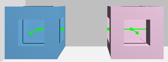
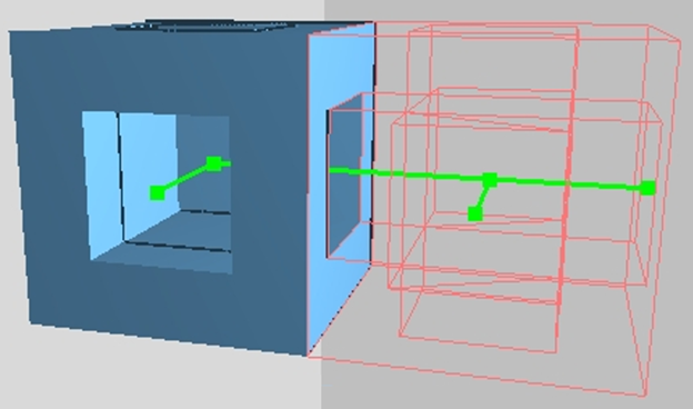
The workspace skeleton is constructed differently depending on the environment. For example, a medial-axis skeleton can easily be constructed for a 2-dimensional environment like the 2D narrow passage in Figure 4(a). In 3D cases like the extended Z tunnel and the grid maze, structures like the mean curvature skeleton [12] can be used to show the connectivity of the workspace. In such environments, however, the default graph may contain long curved edges that do not indicate the changes in the topology of the workspace. For example, a tunnel with a $90^{\circ}$ turn may be represented by a long curved edge with no indication of the change in direction.

Instead of constructing an environment and computing a skeleton afterward, we simultaneously built an environment and skeleton. For simplicity, we create an environment with $90^{\circ}$ angles using cubic structures as building blocks. Considering orientation, there are $2^{6}$ ways to construct a cube with varying tunnels leading outwards. After designing the blocks, a skeleton is constructed for each block based on the tunnel openings, as shown in Figure 5(a). When blocks are paired, their respective skeletons are joined to make a connected graph representing the new topology (Figure 5(b)).

IV-C Experimental Setup

In each environment, a query was set to evaluate the ability of the RRT  variant to solve an accessibility problem in that environment. We pre-computed different types of skeletons and annotated them with clearance for all the problems. The results do not report the time to compute a workspace skeleton since they are incurred only once. However, the time to prune and direct the skeleton is reported in the run time. Each algorithm was given the same amount of time to solve the queries, ranging from 20 seconds to 300, depending on the problem’s difficulty. We report the time to solve the query and its path length as a proxy for path cost.

The experiments were executed on a desktop computer with an Intel Core i7-3770 CPU at 3.4 GHz, 16 GB of RAM, running CentOS 7, and the GNU g++ compiler version 4.8.5. All methods were implemented in our C++ Parasol Planning Library (PPL) [14] developed in the Parasol Lab at the University of Illinois at Urbana-Champaign. Roadmap validation was done with the PQP-SOLID collision detection method [15].

IV-D Discussion

TABLE I: Graph size, success rate, and planning cost comparisons for the tested environments

Environment Number of vertices Collision Detection Calls Completed seeds ($\%$) RRT EET DR-RRT HAS-RRT RRT EET DR-RRT HAS-RRT RRT EET DR-RRT HAS-RRT Simple Passage avg 460.71 1,197.38 57.51 20.0 6,139.4 10,420.15 708.11 389.94 100 62.85 100 100 std 418.93 1,582.71 13.522 3.53 4,355.01 12,629.61 136.73 54.01 Grid Tunnels avg 85.97 16.41 438.77 20.77 5,366.66 1,319.56 8,013.34 1,484.71 100 97.14 100 100 std 59.91 1.26 76.79 13.36 2,816.40 178.81 1,093.73 364.51 Extended Z Tunnel avg 610.86 53.80 502.03 55.29 16,296.2 3,821.61 7,329.06 1,983.29 100 94.29 100 100 std 187.39 4.23 63.77 6.73 3,841.94 203.32 706.90 138.91 Grid Mining avg 387.06 339.12 1,686.86 129.71 35,563.31 18,056.35 28,854.37 5,751.89 11.43 91.43 77.14 100 std 37.26 732.871 90.24 2.35 2,179.22 21,433.10 1,136.77 151.26 Grid Maze avg NaN NaN 3630.0 892.34 NaN NaN 71,025.89 26,145.86 0 0 100 100 std NaN NaN 342.63 194.14 NaN NaN 7,632.66 4,896.17 DhaA avg 229.91 19.06 239.63 80.30 57,272.47 142,878.35 51,531.46 21,485.78 97 49 100 77 std 210.03 3.33 246.47 147.92 74,723.10 1,711,472.17 47,227.46 35,127.74

(a) Run time in seconds

(b) Path cost (path edge weights)

Figure 6: Run time and path cost comparisons for the tested robotics environments

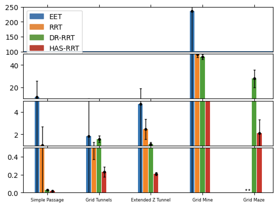
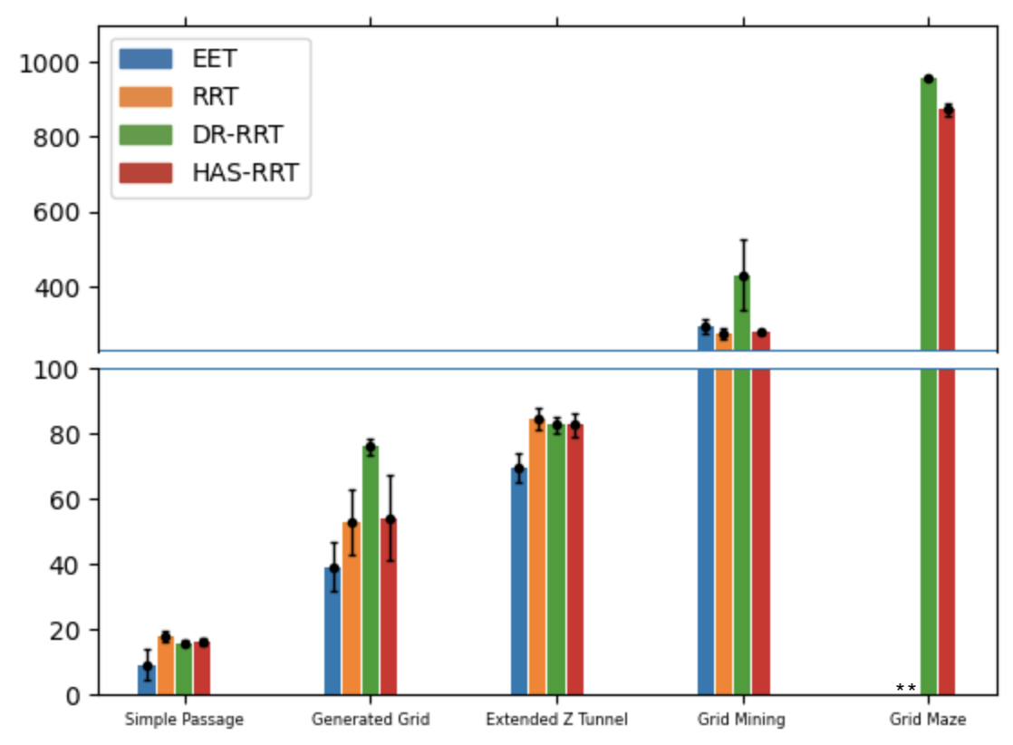
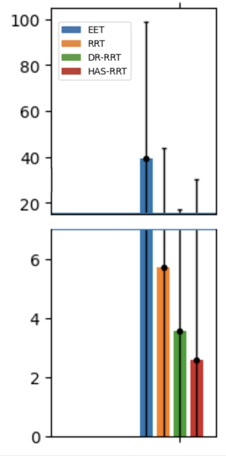
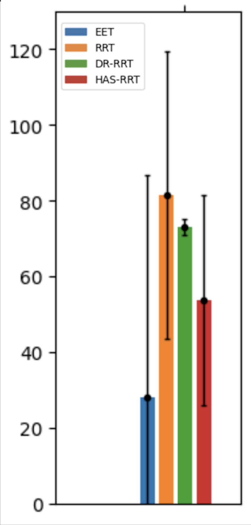
The experimental results in Figure 6, 7 and Table I show the importance of using a workspace skeleton to guide planning and the significant advantage of using hierarchical planning with guidance. The comparative results show that DR-RRT takes longer than HAS-RRT and is not consistently faster than basic RRT or EET. In addition, although EET returns paths with the lowest cost, its success rate is worse than others in most environments, and it is sensitive to parameter tuning.

In the simple passage environment, HAS-RRT outperformed the other guided strategies, thanks to the long successful extension it attempts in the narrow passage with the skeleton’s guidance. DR-RRT locally explores each edge, increasing its sampling failures in the narrow passage. EET takes longer for the wavefront expansion to discover and explore the narrow passage randomly, but the resulting guidance yields a better path cost.

A similar trend can be seen in the Extended Z Tunnel and grid mining environments. These examples highlight one of the main strengths of HAS-RRT: prioritizing paths indicated by the workspace guidance and only sampling if a naive extension fails. By following the guidance of a good skeleton, the runtime of HAS-RRT is greatly minimized while maintaining a competitive path cost.

In the grid tunnel environment, HAS-RRT runs faster than DR-RRT and EET. In addition, DR-RRT  is outperformed by Basic RRT, which shows the second strength of HAS-RRT: adjusting planning when the guidance of the workspace skeleton is poor.

The grid mine environment shows the scalability of HAS-RRT. In this more complex environment, Basic RRT only solved 11% of the 35 random seeds. HAS-RRT even performs better than DR-RRT, because it simply follows the guidance from the long skeleton edges rather than fully exploring each edge.

The grid maze environment is notoriously difficult and was only successfully solved by DR-RRT and HAS-RRT (of the 35 seeds). This environment has curved edges (as shown in Figure 4(e)), even though the environment’s tunnels are straight. From this, we can see two more strengths of HAS-RRT: While HAS-RRT works best with straight-edged workspace skeletons, it performs well on other types of skeletons due to the method’s exploration when necessary. Additionally, as evidenced by HAS-RRT’s lower path cost and faster runtime compared to DR-RRT, HAS-RRT still uses more information from the skeleton than its competitors.

EET’s path costs are comparable and competitive to HAS-RRTbecause the Wavefront expansion guarantees any path to be centered in an environment. However, EET’s runtime is much higher than the other methods because the wavefront expansion is built probabilistically and thus must be recomputed for each seed. Additional investigation shows that the wavefront expansion’s build time is highly sensitive to the complexity of the environment and query: build times for the protein environment were small compared to total runtime (2.26% on average) while build times for the Generated Grid environment averaged 67.73% of the total runtime and for the Extended Z Tunnel averaged 84.53%.

IV-E Protein-Ligand binding site accessibility

(a) The dhaa protein.

(b) Run time in seconds

(c) Path cost (path edge weights)

Figure 7: Run time and path cost comparisons for the DhaA protein

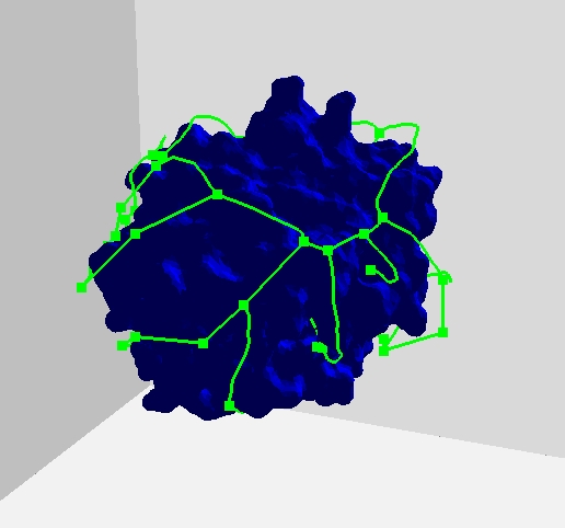
In addition to the robotics environments, we tested the algorithms on an application of computational biology. The DhaA protein environment (Figure 7(a)) shows an example of a protein-ligand binding problem. In this application, the robot is a ligand that aims to access and exit from a protein binding site by finding the exit tunnels that connect it to the protein’s surface. The protein has many dead-end tunnels, making the workspace skeleton indispensable to finding a solution quickly.

We obtain protein data from the protein data bank (PDB)[16] and construct their geometric structure using CHIMERA [17]. A skeleton representing the protein’s free space was constructed using CGAL’s built-in mean curvature skeleton algorithm. Figure 7(a) shows the skeleton in blue with its workspace skeleton.

In the DhaA protein environment, we observe the same trend from the robotics experiments. Figure 7 shows that HAS-RRT has the best run time to find a path through an exit tunnel connecting the binding site to the outer surface. In addition, HAS-RRTś path is the second best after EET.

V conclusion

In conclusion, this research introduces a novel hierarchical RRT strategy enhanced by an annotated workspace skeleton designed to address intricate motion planning challenges within complex environments. By strategically prioritizing paths available within the workspace, our proposed Hierarchical Annotated-Skeleton guided RRT approach leverages guidance from a workspace graph to efficiently guide the RRT’s expansion process. This guidance, rooted in the workspace skeleton, ensures the hierarchical progression of the tree expansion even in scenarios where the skeleton’s guidance is partially uncertain. This results in a roadmap that selectively explores critical regions within the $\mathcal{C}_{space}$, progressively uncovered through hierarchical adjustments relying on workspace guidance.

With comprehensive empirical analysis, we have substantiated the efficacy of our method by benchmarking it against alternative workspace-guided strategies within demanding environments. Our experimental findings underscore the value of incorporating workspace information into motion planning problems where relevant. Importantly, among workspace-guided strategies, HAS-RRT  stands out as the optimal choice, yielding dependable paths faster than established RRT methods.

References

- [1] B. Englot and F. S. Hover, “Sampling-based coverage path planning for inspection of complex structures,” in Proc. Int. Conf. Automated Planning and Scheduling, 2012.
- [2] D. Brutlag, M. Apaydin, C. Guestrin, D. Hsu, C. Varma, A. Singh, and J.-C. Latombe, “Using robotics to fold proteins and dock ligands.” in Bioinformatics, 2002, p. 18:S74.S83.
- [3] J. H. Reif, “Complexity of the mover’s problem and generalizations,” in Proc. IEEE Symp. Found. Comp. Sci. (FOCS), San Juan, Puerto Rico, Oct. 1979, pp. 421–427.
- [4] S. M. LaValle and J. J. Kuffner, “Rapidly-exploring random trees: Progress and prospects,” in New Directions in Algorithmic and Computational Robotics. A. K. Peters, 2001, pp. 293–308, (WAFR 2000).
- [5] J. Denny, R. Sandström, A. Bregger, and N. M. Amato, “Dynamic region-biased exploring random trees,” in Alg. Found. Robot. XII. Springer, 2020, (WAFR ‘16).
- [6] M. Rickert, O. Brock, and A. Knoll, “Balancing exploration and exploitation in motion planning,” in 2008 IEEE International Conference on Robotics and Automation, 2008, pp. 2812–2817.
- [7] L. E. Kavraki, P. Švestka, J. C. Latombe, and M. H. Overmars, “Probabilistic roadmaps for path planning in high-dimensional configuration spaces,” IEEE Trans. Robot. Automat., vol. 12, no. 4, pp. 566–580, Aug. 1996.
- [8] H. Kurniawati and D. Hsu, “Workspace importance sampling for probabilistic roadmap planning,” in Proc. IEEE Int. Conf. Intel. Rob. Syst. (IROS), vol. 2, Sept. 2004, pp. 1618–1623.
- [9] J. Berg and M. Overmars, “Using workspace information as a guide to non-uniform sampling in probabilistic roadmap planners,” in Proc. IEEE Int. Conf. Robot. Autom. (ICRA), 2004, pp. 453–460.
- [10] H. Kurniawati and D. Hsu, “Workspace-based connectivity oracle - an adaptive sampling strategy for prm planning,” in Alg. Found. Robot. VII. Springer, 2008, pp. 35–51, (WAFR ‘06).
- [11] E. Plaku, L. Kavraki, and M. Vardi, “Motion planning with dynamics by a synergistic combination of layers of planning,” IEEE Trans. Robot., vol. 26, no. 3, pp. 469–482, June 2010.
- [12] S. Bhattacharya, M. Likhachev, and V. Kumar, “Topological constraints in search-based robot path planning,” Autonomous Robots, vol. 33, no. 3, 2012.
- [13] H. Doraiswamy and V. Natarajan, “Efficient algorithms for computing reeb graphs,” Comput. Geom. Theory Appl., vol. 42, no. 6-7, pp. 606–616, Aug. 2009. [Online]. Available: http://dx.doi.org/10.1016/j.comgeo.2008.12.003
- [14] “PPL, Parasol Planning Library,” https://gitlab.engr.illinois.edu/parasol-group/parasol/open-ppl.
- [15] E. Larsen, S. Gottschalk, M. Lin, and D. Manocha, “Fast proximity queries with swept sphere volumes,” University of N. Carolina, Chapel Hill, CA, Technical Report TR99-018, 1999.
- [16] “The Protein Data Bank,” http://www.rcsb.org/pdb/.
- [17] E. F. Pettersen, T. D. Goddard, C. C. Huang, G. S. Couch, D. M. Greenblatt, E. C. Meng, and T. E. Ferrin, “Ucsf chimera: A visualization system for exploratory research and analysis,” Journal of Computational Chemistry, vol. 25, no. 13, pp. 1605–16 012, 2004.