Heuristic Search for Path Finding with Refuelling

Abstract

This paper considers a generalization of the Path Finding (PF) with refueling constraints referred to as the Refuelling Path Finding (RF-PF) problem. Just like PF, the RF-PF problem is defined over a graph, where vertices are gas stations with known fuel prices, and edge costs depend on the gas consumption between the corresponding vertices. RF-PF seeks a minimum-cost path from the start to the goal vertex for a robot with a limited gas tank and a limited number of refuelling stops. While RF-PF is polynomial-time solvable, it remains a challenge to quickly compute an optimal solution in practice since the robot needs to simultaneously determine the path, where to make the stops, and the amount to refuel at each stop. This paper develops a heuristic search algorithm called $\text{Refuel A}^{*}$ ($\text{RF-A}^{*}$) that iteratively constructs partial solution paths from the start to the goal guided by a heuristic function while leveraging dominance rules for state pruning during planning. $\text{RF-A}^{*}$ is guaranteed to find an optimal solution and runs more than an order of magnitude faster than the existing state of the art (a polynomial time algorithm) when tested in large city maps with hundreds of gas stations.

I Introduction

Given a graph with non-negative edge costs, the well-known Path Finding (PF) problem seeks a minimum-cost path from the given start vertex to a goal vertex. This paper considers a Refueling Path Finding (RF-PF) problem, where the vertices represent gas stations with known fuel prices, and the edge costs indicate the gas consumption when moving between vertices. The fuel prices at vertices may be different and are fixed over time. RF-PF seeks a start-goal path subject to a limited gas tank and a limited number of refuelling stops while minimizing the fuel cost along the path (Fig. 1).

RF-PF is also called the Gas Station Problem [6, 18, 4, 13] in the literature. It arises in applications such as path-finding for electric vehicles between cities  [15, 1, 2] and package delivery using an unmanned vehicle [7, 5], where a robot needs to move over long distance when refuelling becomes necessary. While RF-PF is polynomial time solvable [6, 13, 4], it remains a challenge to quickly compute an optimal solution in practice since the robot needs to simultaneously determine the path, where to make the stops, and the amount of refuelling at each stop.

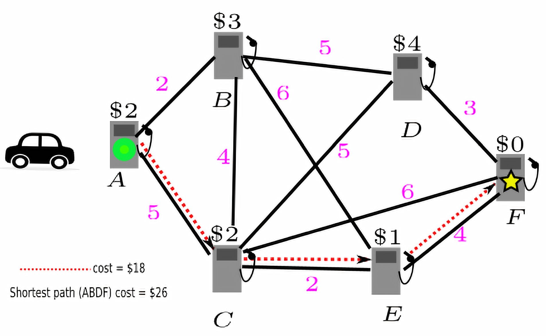
Figure 1: An illustrative example of RF-PF. This graph consists of six vertices representing gas stations, each associated with a gas price and each edge with its fuel expenditure. The objective is to find a minimum-cost path from start to goal. The figure shows an optimal solution (ACEF) using a dotted red line and the fuel cost taken by the shortest path (ABDF). Note that the shortest path does not incur the lowest fuel cost. Along the optimal solution ACEF, the cost of refuelling at each vertex is: $\$10$ at A, $\$14$ at C, $\$18$ at E.

This paper focuses on exact algorithms that can solve RF-PF to optimality. In [6], a dynamic programming (DP) approach is developed to solve RF-PF to optimality, which has been recently further improved in terms of its theoretic runtime complexity [13]. This DP approach identifies a principle regarding the amount of refuelling the robot should take at each stop along an optimal path, which allows the construction of a finite state space where dynamic programming can be applied to iteratively find the optimal refuelling cost at each state until an optimal solution is found.

To expedite computation, this paper develops a new heuristic search algorithm called $\text{RF-A}^{*}$, which iteratively constructs partial solution paths from the start vertex to the goal guided by a heuristic function. $\text{RF-A}^{*}$ gains computational benefits over DP in the following aspects. First, $\text{RF-A}^{*}$ never explicitly constructs the entire state space as DP does and only explores states that are needed for the search. Second, $\text{RF-A}^{*}$ uses a heuristic to guide the search, limiting the fraction of state space to be explored before an optimal solution is found. Third, taking advantage of our prior work in multi-objective search [16, 17], $\text{RF-A}^{*}$ introduces a dominance rule to prune partial solutions during the search, which saves computation. $\text{RF-A}^{*}$ is guaranteed to find an optimal solution.

We compare $\text{RF-A}^{*}$ against DP in real-world city maps of various sizes from the OpenStreetMap dataset. Our results show that $\text{RF-A}^{*}$ runs more than an order of magnitude faster than the DP method as tested in maps with hundreds of gas stations. While DP takes up to hundreds of seconds to solve these test instances, $\text{RF-A}^{*}$ often takes less than a second. The fast running speed makes it possible to apply $\text{RF-A}^{*}$ for online planning on a robot with a limited tank in large urban areas. Our software will be open-sourced.

II Related Work

Path planning with refuelling has been investigated from various perspectives. Along a fixed start-goal path, mathematical programming models were developed to decide the refuelling schedule, $i.e.$, where to make the refuel stop and the amount of refuelling [18, 4]. Subsequent research [6, 13] seeks to determine both the path and the refuelling schedule simultaneously, either from a given start to a goal or for all-pair vertices in the graph.

Besides planning start-goal paths, another related problem generalizes the well-known travelling salesman problem and vehicle routing problem with refuelling constraints [6, 9, 19]. Instead of finding a start-goal path, these problems seek a tour that visits multiple vertices subject to a limited fuel tank. This paper only considers finding a start-goal path.

Recently, due to the prevalence of electric vehicles, several variants of RF-PF [11, 9] were proposed to plan paths while considering additional aspects of the vehicle such as moving speeds [8], arrival times [1], and detailed powertrain model [2]. To address them, various approaches were developed, such as dynamic programming [6], greedy method [10], and learning-based approaches [12, 8].

III Problem Statement

Let $G=(V,E)$ denote a directed graph, where each vertex $v\in V$ represents a gas station, and each edge $(u,v)\in E$ denotes an action that transits the robot from vertex $u$ to $v$. Each edge $(u,v)\in E$ is associated with a non-negative real value $d(u,v)\in\mathbb{R}^{+}$, which represents the amount of fuel needed to traverse the edge from $u$ to $v$. The robot has a fuel capacity $q_{max}\in\mathbb{R}^{+}$ representing the maximum amount of fuel it can store in its tank. Let $c:V\rightarrow[0,\infty]$ denote the refuelling price per unit of fuel at each vertex in $v\in V$.

Let a path $\pi(v_{1},v_{\ell})=(v_{1},v_{2},\dots,v_{\ell})$ be an ordered list of vertices in $G$ such that every pair of adjacent vertices in $\pi(v_{1},v_{\ell})$ is connected by an edge in $G$, i.e., $(v_{k},v_{k+1})\in E,k=1,2,\dots,\ell-1$. Let $g(\pi)$ denote total fuel cost along the path; specifically, let a non-negative real number $a(v)\in\mathbb{R}^{+}$ denote the amount of refuelling taken by the robot at vertex $v$, then $g(\pi)=\sum_{k=1,2,\dots,\ell}a(v_{k})c(v_{k})$.

In practice, the robot often has to stop to refuel, which slows down the entire path execution time. Therefore, let $k_{max}\in\mathbb{Z}^{+},k_{max}>1$ denote the maximum number of refuelling stops the robot is allowed to make along its path.

Definition 1 (Refueling Path Finding (RF-PF)).

Given a pair of start and goal vertex $v_{o},v_{g}\in V$, the robot has zero amount of fuel at $v_{o}$ and must refuel to travel. The RF-PF problem seeks a path $\pi$ from $v_{o}$ to $v_{g}$ such that $g(\pi)$ is minimized while the number of refuelling stops along $\pi$ is no larger than $k_{max}$.

Remark 1.

In Def. 1, we only need to consider the case where the robot starts with zero fuel at $v_{o}$ for the following reason. If the robot starts with $q_{0}$ fuel at $v_{o}$, one can always construct a new problem where the robot starts with zero fuel as follows. First, let $G^{\prime}$ denote a new graph whose vertex set is $V^{\prime}=V\cup\{v_{o}^{\prime}\}$, where $v_{o}^{\prime}$ is only connected to $v_{o}$ with $d(v_{o}^{\prime},v_{o})=q_{max}-q_{0}$ and $c(v_{o}^{\prime})=0$. Then, in $G^{\prime}$, the robot starts with zero fuel, and the goal is to find a minimum cost path $\pi^{\prime}$ in $G^{\prime}$ from $v_{o}^{\prime}$ to $v_{g}$. Following $\pi^{\prime}$, the robot arrives at $v_{o}$ with $q_{0}$ fuel, and the remaining path is the desired solution. We can also assume $c(v_{g})=0$ since in an optimal solution, the robot never refuels at the goal vertex and taking $c(v_{g})=0$ does not change an optimal solution.

IV Method

This section introduces $\text{RF-A}^{*}$, a heuristic search approach to find an optimal solution for RF-PF. It initiates at $v_{o}$ and systematically explores potential paths from $v_{o}$ towards $v_{g}$ while minimizing the overall fuel cost. The heuristics help estimate the remaining cost to the goal and guide the search. $\text{RF-A}^{*}$ also considers the fuel tank limit $q_{max}$ and the refuelling stop limit $k_{max}$, by comparing two paths that reach the same vertex using multiple criteria. During the search, $\text{RF-A}^{*}$ maintains an open set of candidate labels that are to be expanded, similar to A* [14]. It continues searching until finding an optimal path satisfying the constraints. A toy example of the search process is provided in Fig. 2.

IV-A Notations and Background

IV-A1 Basic Concepts

In RF-PF, there can be multiple paths from $v_{o}$ to a vertex $v$, and to differentiate them, we use the notion of labels. A label $l=(v,g,q,k)$ consists of a vertex $v\in V$, a non-negative real number $g\in\mathbb{R}^{+}$ that represents the cost-to-come from $v_{o}$ to $v$, a non-negative real number $q\in\mathbb{R}^{+}$ that represents the amount of fuel remaining at $v$ before refuelling. We use $v(l),g(l),q(l),k(l)$ to denote the respective component of a label. To compare labels, we use the following notion of label dominance.

Definition 2.

Given two labels $l,l^{\prime}$ with $v(l)=v(l^{\prime})$, label $l$ dominates $l^{\prime}$ if the following three inequalities hold: (i) $g(l)\leq g(l^{\prime})$ , (ii) $q(l)\geq q(l^{\prime})$ and (iii) $k(l)\leq k(l^{\prime})$.

If $l$ dominates $l^{\prime}$, then $l^{\prime}$ can be discarded during the search, since for any path from $v_{o}$ via $l^{\prime}$ to $v_{g}$, there must be a corresponding path from $v_{o}$ via $l$ to $v_{g}$ with the same or smaller cost. Otherwise, both $l$ and $l^{\prime}$ are non-dominated by each other. Let $\mathcal{F}(v),v\in V$ denote the frontier set at $v$, a set of labels that reach $v$ and are non-dominated by each other. Additionally, the procedure $\textsl{CheckForPrune}(l)$ compares $l$ against all existing labels in $\mathcal{F}(v(l))$.

Similarly to A* search [3], let $h(l)$ denote the $h$-value of label $l$ that estimates the cost-to-go from $v$ to $v_{g}$. We further explain the heuristic in Sec. IV-B2. Let $f(l)=g(l)+h(l)$ be the $f$-value of label $l$. Let OPEN denote a priority queue of labels, where labels are prioritized based on their $f$-values from the minimum to the maximum.

IV-A2 Review of Dynamic Programming Method [6]

A major difficulty in RF-PF is determining the amount of refuelling at each vertex during the search, a continuous variable that can take any value in $[0,q_{max}]$. To handle this difficulty, we borrow the following lemma from [6], which provides an optimal strategy for refuelling at any vertex.

Lemma 1 (Optimal Refuelling strategy).

Given refill stops $v_{1},\cdots,v_{n}$ along an optimal path using at most $k_{max}$ stops. At $v_{g-1}$, which is the stop right before $v_{g}$, refill enough to reach $v_{g}$ with an empty tank. Then, an optimal strategy to decide how much to refill at each stop for any $n<g-1$ :

• if $c(v_{n})<c(v_{n+1})$, then fill up entirely at $v_{n}$.

• if $c(v_{n})\geq c(v_{n+1})$, then fill up enough to reach $v_{n+1}$.

The intuition behind Lemma 1 is that the robot either fills up the tank if the next stop has a higher fuel price, or fills just enough amount of fuel to reach the next stop if the next stop has a lower price. By doing so, the robot minimizes its accumulative fuel cost. A detailed proof is given in [6].

Algorithm 1 $\text{RF-A}^{*}$

1:ComputeReachableSets()

2:ComputeHeuristic($v_{g}$)

3:$l_{o}\leftarrow(v_{o},g=0,q=0,k=0)$, ${f}(l_{o})\leftarrow{0}+{h}(l_{o})$

4:$parent(l_{o})\leftarrow NULL$

5:Add $l_{o}$ to OPEN

6:$\mathcal{F}(v)\leftarrow\emptyset,\forall v\in V$

7:while OPEN $\neq\emptyset$ do

8:    pop $l=(v,g,q,k)$ from OPEN

9:    if CheckForPrune($l$,$\mathcal{F}(v(l))$) then

10:         continue     

11:    add l to $\mathcal{F}(v(l))$

12:    if $v(l)=v_{g}$ then

13:         continue     

14:    if $k=k_{max}$ then

15:         continue     

16:    break

17:    for all $v^{\prime}\in$ GetReachableSet($v(l)$) do

18:         if $c(v^{\prime})>c(v)$ then

19:             $g^{\prime}\leftarrow g(l)+(q_{max}-q(l))c(v)$

20:             $q^{\prime}\leftarrow q_{max}-d(v,v^{\prime})$

21:             $k^{\prime}\leftarrow k+1$

22:         else

23:             if $d(v^{\prime},v)>q(l)$ then

24:                 $g^{\prime}\leftarrow g(l)+(d(v^{\prime},v)-q(l))c(v)$

25:                 $q^{\prime}\leftarrow 0$

26:                 $k^{\prime}\leftarrow k+1$                       

27:         $l^{\prime}\leftarrow(v^{\prime},g^{\prime},q^{\prime},k^{\prime})$

28:         $g(l^{\prime})\leftarrow g^{\prime}$

29:         if CheckForPrune($l^{\prime}$,$\mathcal{F}(v(l))$) then

30:             continue          

31:         ${f}(l^{\prime})\leftarrow{g}(l^{\prime})+{h}(v(l^{\prime}))$

32:         $parent(l^{\prime})\leftarrow l$

33:         add $l^{\prime}$ to OPEN     

34:return Reconstruct($v_{d}$)

Algorithm 2 ComputeReachableSets

1:$Reach(v)\leftarrow\emptyset,\forall v\in V$

2:for $v\in V$ do

3:    $d^{*}(u)\leftarrow\infty,\forall u\in V$

4:    $d^{*}(v)\leftarrow 0$

5:    Add $v$ to OPEN_v

6:    while OPEN_v $\neq\emptyset$ do

7:         pop $u$ from OPEN_v

8:         if $d^{*}(u)>q_{max}$ then

9:             continue

10:         else

11:             add $u$ to $Reach(v)$          

12:         for $u^{\prime}\in$ GetSucc($u$) do

13:             if $u^{\prime}\in Reach(v)$ then

14:                 continue              

15:             if $d^{*}(u^{\prime})>d^{*}(u)+d(u,u^{\prime})$ then

16:                 $d^{*}(u^{\prime})\leftarrow d^{*}(u)+d(u,u^{\prime})$

17:                 add $u^{\prime}$ to OPEN_v                           

Algorithm 3 $\textsl{CheckForPrune}(l,\mathcal{F}(v(l)))$

1:INPUT: A label $l$ and $\mathcal{F}(v(l))$, the frontier set at vertex $v(l)$.

2:for all $l^{\prime}\in\mathcal{F}(v(l))$ do

3:    if $g(l^{\prime})\leq g(l)$ and $q(l^{\prime})\geq q(l)$ and $k(l^{\prime})\leq k(l)$  then

4:         return true $\triangleright$ $l$ should be pruned.     

5:return false$\triangleright$ $l$ should not be pruned.

We now summarize the dynamic programming (DP) algorithm for RF-PF from [6]. This DP defines a state space where each state is $(v,k,q)$ with $v\in V$, $k$ denoting the number of stops and $q$ denoting the gas level. For each state, let $A(v,k,q)$ represent the minimal cost to traverse from vertex $v$ to the goal $v_{g}$, within $k$ refuelling stops, and starting with $q$ units of fuel. With the help of Lemma 1, for each $v\in V$, there is only a finite number of possible values that $q$ can take, which is bounded by $|V|$. As a result, the state space is finite since each of $v,k,q$ can take a finite number of possible values. The boundary condition of the DP method for any vertex $v$, $A(v,1,q)$, is governed by a cost of $(d_{vg}(u)-q)*c(v)$ if $q\leq d_{vg}(u)\leq q_{max}$, and $\infty$ otherwise. Then, this method uses the dynamic programming principle to iteratively compute $A(v,k,q)$ for all possible $v,k,q$ and returns an optimal solution. In [6], two methods are presented to compute $A(v,k,q)$. The first method (referred to as the naive version), evaluates $A(v,k,q)$ for each vertex and stop, incurring a time complexity of $O(k_{max}n^{3})$, spending $O(n)$ time on each state $(v,k,q)$. The second method ameliorates this complexity to $O(k_{max}n^{2}\log(n))$ by employing an amortized time of $O(n\log(n))$ per state. We consider the second method for comparison.

IV-B $\text{Refuel A}^{*}\text{ Algorithm}$

$\text{RF-A}^{*}$ (Alg. 1) takes $G$ and $q_{max}$, $v_{o}$, $v_{g}$, and $k_{max}$ as the inputs. It begins by calling Alg. 2 ComputeReachableSets(explained in  IV-B3) to compute the set of all vertices that the robot can travel to from any vertex $u$ given a full-tank. Subsequently, to compute the heuristic which gives the amount of fuel needed to reach $v_{g}$ from any other vertex, it runs an exhaustive backward Dijkstra search from $v_{g}$. We elaborate on the heuristic computation in Sec. IV-B2. After the Dijkstra, it initiates the label $l_{o}=(v_{o},g=0,q=0,k=0)$ at vertex $v_{o}$ with the ${f}$-value, ${f}(l_{o})={h}(l_{o})$, and inserts it into OPEN. Moreover, the frontier set $\mathcal{F}(v)$ is initialized as a null ($\emptyset$) set.

The search process is from Lines 8-30. In each iteration, the label with the lowest ${f}(l)$ value is popped from the OPEN set for further processing. Then this label is checked for dominance against existing labels in $\mathcal{F}(v(l))$ using CheckForPrune. This procedure employs Def. 2 to compare the $g$, $q$ and $k$ values of the popped label against other labels in $\mathcal{F}(v(l))$.

If the selected label is unpruned, it is added to the frontier set. Subsequently, the algorithm checks if $v(l)=v_{g}$, which signifies that the label $l$ has established a solution with minimum cost, and the search process terminates. The algorithm also confirms whether the $k_{max}$ stops limit has been reached. In cases where $v(l)\neq v_{g}$ and $k^{\prime}\neq k_{max}$, the label is expanded, which generates new labels for all reachable vertices from $v(l)$ within graph $G$. This involves a for loop iterating over each reachable vertex, creating a new label $l^{\prime}$ with new $g^{\prime},q^{\prime},k^{\prime}$. The amount of refuelling is determined using Lemma 1, and the corresponding accumulative fuel cost $g^{\prime}$ is computed. Finally, the algorithm employs CheckForPrune to check the for dominance. If $l^{\prime}$ is not pruned, then it is added to the OPEN set for future expansion.

IV-B1 ComputeReachableSets

This algorithm finds all vertices $v^{\prime}\in V$ that the robot with a full tank can reach from vertex $v$. This algorithm aims to find all successor vertices that $\text{RF-A}^{*}$ needs to consider when expanding a label. Specifically, Alg. 2, initializes $\text{Reach}(v)$, an empty set for all $v\in V$. With each iteration, it designates a vertex $v$ and runs a Dijkstra search from $v$ to all other vertices in $G$ to find vertices that are reachable without refuelling. Line 3-17 is this Dijkstra search process starting from a specific vertex $v$. This algorithm involves iterating through vertices in $V$ and traversing their successors to update the distances.

IV-B2 Heuristic Determination

A possible way to compute the heuristic is to first run an exhaustive backward Dijkstra search on $G$ from $v_{g}$ to any other vertices in $G$ using $d(u,v)$ as the edge cost (ignoring the fuel tank limit of the robot and the refuelling cost). After this Dijkstra search, let $d_{v_{g}}(v)$ denote the cost of a minimum cost path from $v$ to $v_{g}$. Let $c_{min}:=\min_{v\in V-\{v_{g}\}}(c(v))$ denote the minimum refuel cost in $G$. Then, let $h(l)=\max\{(d_{v_{g}}-q(l))c_{min},\;0\}$ be the $h$-value of label $l$. When computing this heuristic, the tank limit of the robot is ignored and the fuel price at any station is a lower bound of the true price at that station. As a result, $h(v)$ provides a lower bound of the total fuel cost to reach $v_{g}$ from $v$. We therefore have the following lemma.

Lemma 2 (Admissible Heuristic).

The heuristic, $h(l)=max\{(d_{v_{g}}-q(l))c_{min},0\}$, is admissible.

IV-B3 $\textsl{CheckForPrune}(l,v(l))$

This can be seen in Alg. 3. It is responsible for the dominance check for each label $l$ against all labels contained in $\mathcal{F}(v(l))$ of a vertex $v$. CheckForPrune checks the label for dominance using Def. 2. Alg. 3 operates within the frontier set $\mathcal{F}$, with its efficiency determined by the size of $|\mathcal{F}(v(l))|$, leading to a complexity of $O(|\mathcal{F}(v(l))|)$.

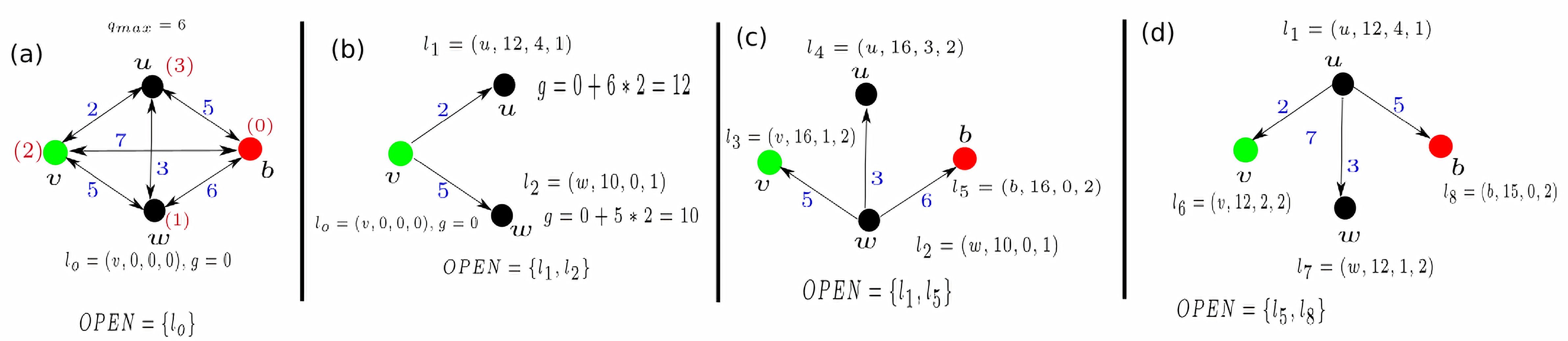
Figure 2: A toy example showing the $\text{Refuel A}^{*}$ with four vertices. (a) The entire graph has four vertices $(v,u,b\text{ and }w)$, with fuel cost in red, fuel spent in blue, $q_{max}=6$ and $k_{max}=2$. The labels associated with each vertex are $l_{vertex}=(u,q,g,k)$. (b) The first iteration in the search case is where $l_{o}$ is popped from OPEN. Around each vertex, its corresponding label is provided. (c) The next iteration in the search is provided, where $l_{2}$ is popped, and (d) shows the last case when $l_{5}$ is popped. Optimal path is $v\to u\to b$

IV-C $\text{RF-A}^{*}$ Example

The working of Alg. 1 $\text{RF-A}^{*}$ is shown in Fig. 2. It considers a graph $G$ with four vertices $u,v,w,\text{and }b$. The source is $v$, and goal $b$. The label $l_{o}=(v,0,0,0)$ is initiated and inserted into the OPEN set. In the first search iteration, as seen in Fig. 2(b), $l_{0}$ is popped from OPEN. Since $l_{0}$ does not belong to the goal vertex, its reachable vertices are processed and given labels $l_{1}=\{u,12,4,1\}$ and $l_{2}=\{w,10,0,1\}$. To compute $l_{1}$, we can see that since $c(u)>c(v)$ robot fills up the gas tank and then moves to $u$ which causes $g(l_{1})=12$, $q(l_{1})=6-2=4$ and $k(l_{1})=1$. Alternately, $c(w)\leq c(u)$, so the robot only fills up the amount needed to go to $w$, thus $g(l_{2})=10$, $q(l_{2})=5-5=0$ and $k(l_{2})=1$. Both $l_{1}$ and $l_{2}$ are inserted into OPEN as there are no labels to compare them against. Next, Fig. 2(c), we extract $l_{2}$ from OPEN, which has the lowest $f$-value in OPEN, and follow the same process for generating labels $l_{3},l_{4}\text{and }l_{5}$ corresponding to vertices $v,u$ and $b$ with $k(l_{3})=k(l_{4})=k(l_{5})=2$. Subsequently, we compare them against the labels $l_{0}$ and $l_{1}$ and notice that $l_{3}$ is pruned by $l_{o}$, and $l_{4}$ by $l_{1}$ using CheckForPrune. Hence, only $l_{5}$ is inserted into the OPEN set, that is, OPEN = $\{l_{1},l_{5}\}$. In the final iteration, seen in Fig. 2 (d), we pop label $l_{1}$ from the OPEN since $g(l_{1})$ has the lowest value and processes its reachable vertices. We process and assign labels of $l_{6},l_{7}$ and $l_{8}$ to vertices $v,w$ and $b$ and set stops $k(l_{6})=k(l_{7})=k(l_{8})=2$. Once $l_{6}$ and $l_{7}$ are checked for dominance against $l_{o},l_{2}$, we can see that they get pruned by $l_{0}$ and $l_{2}$, respectively. Therefore, only $l_{8}$ is inserted into the OPEN set. Finally, in the OPEN set, we see that $g(l_{8})<g(l_{5})$ with $k(l_{5})=k(l_{8})=2=k_{max}$. Hence, it is popped from OPEN and claimed as an optimal solution. Therefore, the path and cost being $v\to u\to b$ and $15$.

IV-D Analysis

In the worst case, $\text{RF-A}^{*}$ may have the same run-time complexity as the naive version of the DP algorithm, $O(k_{max}n^{3})$. This scenario for $\text{RF-A}^{*}$ may occur when the heuristic is absent (e.g. $h(v)=0$ for any $v\in V$), dominance pruning does not occur, and all possible labels are expanded. However, as shown in Sec. V, in practice, $\text{RF-A}^{*}$ is often much faster than the DP method. The following theorem summarize this property.

Theorem 1.

$\text{RF-A}^{*}$ has polynomial worst-case run-time complexity.

In Alg. 1, due to Line 14, $\text{RF-A}^{*}$ never expands a label $l$ with $k(l)=k_{max}$. As a result, $\text{RF-A}^{*}$ never generates labels with more than $k_{max}$ refuelling stops, and the path returned by $\text{RF-A}^{*}$ is feasible, i.e., does not exceed the limit on the number of stops $k_{max}$. The following lemma summarizes this property.

Lemma 3 (Path Feasibility).

The path returned by $\text{RF-A}^{*}$ is feasible.

To expand a label, $\text{RF-A}^{*}$ considers all reachable neighboring vertices as described in Sec. IV-B1 and determine the amount of refuelling via Lines 18-26. With Lemma 1, the expansion of a label $l$ in $\text{RF-A}^{*}$ is complete, in a sense that, all possible actions of the robot, which may lead to an optimal solution, are considered during the expansion. The following lemma summarizes this property.

Lemma 4 (Complete Expansion).

The expansion of a label in $\text{RF-A}^{*}$ is complete.

During the search, if a label is pruned by dominance in CheckForPrune, then this label cannot lead to an optimal solution for the following reasons. If a label $l=(v,g,q,k)$ is dominated by any existing label $l^{\prime}=(v,g^{\prime},q^{\prime},k^{\prime})\in\mathcal{F}(v(l))$. This means that $l$ has a higher cost $g\geq g^{\prime}$, lower remaining fuel $q\leq q^{\prime}$ and has made more stops $k\geq k^{\prime}$ than $l^{\prime}$. Assume that expanding $l$ leads to an optimal solution $\pi_{*}$, and let $\pi_{*}(v,v_{g})$ denote the sub-path within $\pi_{*}$ from $v$ to $v_{g}$. Then, another path $\pi^{\prime}$ can be constructed by concatenating the path represented by $l^{\prime}$ from $v_{o}$ to $v$, and $\pi_{*}(v,v_{g})$ from $v$ to $v_{g}$. Path $\pi^{\prime}$ is feasible and its cost $g(\pi^{\prime})\leq g(\pi_{*})$. So, $\pi^{\prime}$ is a better path than $\pi_{*}$, which contradicts with the assumption. We summarize this property with the following lemma.

Lemma 5 (Dominance Pruning).

Any label that is pruned by dominance cannot lead to an optimal solution.

We now show that $\text{RF-A}^{*}$ is complete and returns an optimal solution for solvable instances.

Theorem 2 (Completeness).

For unsolvable instances, $\text{RF-A}^{*}$ terminates in finite time. For solvable instance, $\text{RF-A}^{*}$ returns a feasible solution in finite time.

Proof.

Due to Lemma 1 and that the graph $G$ is finite, only a finite number of possible labels can be generated during the search. With Lemma 4, the expansion of a label is complete, which means, $\text{RF-A}^{*}$ eventually enumerates all possible labels. For an unsolvable instance, $\text{RF-A}^{*}$ terminates in finite time after enumerating all these labels. For solvable instances, due to Lemma 3, $\text{RF-A}^{*}$ terminates in finite time and finds a label that represents a feasible path.

Theorem 3 (Solution Optimality).

For solvable instances, the path returned by $\text{RF-A}^{*}$ is an optimal solution.

Proof.

When a label $l$ is popped from OPEN and claimed as a solution by $\text{RF-A}^{*}$, due to Lemma 2, any other labels in OPEN and their successor labels cannot lead to a cheaper solution than $g(l)$. With Lemma 5, the pruned labels cannot lead to a cheaper solution than $l$.

V Results

V-A Testing and implementation

We compare our $\text{RF-A}^{*}$ against the DP method[6]. Both are implemented in C++17 and tested on a Ubuntu 20.04 laptop with AMD Ryzen 7 4800h 4.3GHz CPU and 16GB RAM.

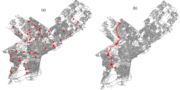
Figure 3: Visualization of the map for Philadelphia, PA, USA, used in testing. (a) showcases the city road network of Philadelphia, where the red dots represent the gas stations. We create a “gas station graph” $G=(V,E)$ for our tests, where $V$ is the set of gas stations, and each edge is a minimum cost path between the corresponding gas stations. We create this graph $G$ using a pre-processing step, and both algorithms ($\text{RF-A}^{*}$ and DP) runs on this $G$ as opposed to the original city road network. (b) shows the solution path returned by our algorithm for one such test case. The agent stops at 5 gas stations before reaching the destination.

V-A1 Data preparation and testing

We use graphs from OpenStreetMap dataset over the USA and Europe, collected using the “osmnx” library in Python. The cities used with the number of gas stations: Philadelphia, PA, USA (61); Austin, TX, USA (87); Phoenix, AZ, USA (178); London, UK (258); and Moscow, Russia (423). We use 20 random start-goal pairs in each city for testing.

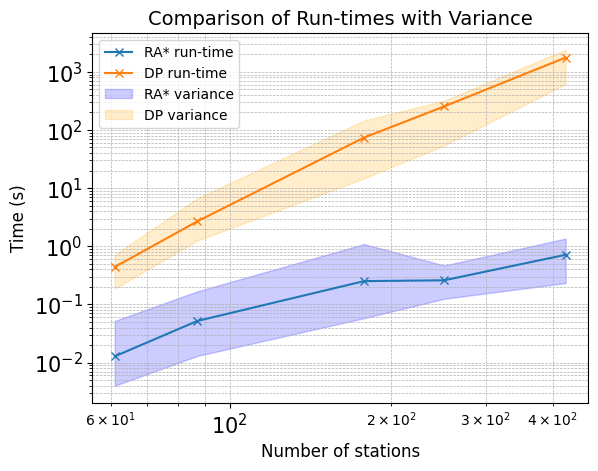
Figure 4: $\log-\log$ plot for runtime (s) comparison between $\text{RF-A}^{*}$ and DP baseline

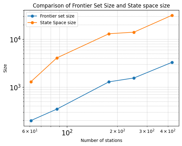
Figure 5: $\log-\log$ plot for size comparison between the size of the mean of the total frontier set size of $\text{RF-A}^{*}$ calculated over 20 tests and the mean of the total state space size of the DP baseline.

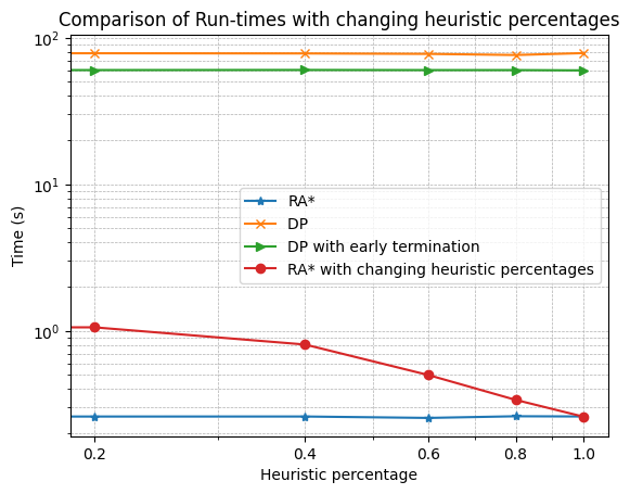
Figure 6: $\log$-plot of the run-time comparison for $\text{RF-A}^{*}$ when heuristic influence is varied from $0-100\%$, and a variant of the DP algorithm with a termination condition for when the goal vertex is reached.

V-B Discussion

From the numerical results shown in Fig. 4, we can see that our algorithm $\text{RF-A}^{*}$ takes significantly less time than the DP baseline [6] to execute and find an optimal solution. The properties of our algorithm which allow for such fast computation are mainly due to the heuristic function, not constructing and exploring the entire search space and the dominance rules, which are explained as follows.

V-B1 Runtime comparison

$\text{RF-A}^{*}$ expedites the computational by avoiding constructing the entire state space. $\text{RF-A}^{*}$ selectively explores the necessary labels for expansion and prunes the labels which get dominated. $\text{RF-A}^{*}$ becomes increasingly advantageous when searching larger graphs. As seen in Fig. 4 on the graph with 400+ stations, $\text{RF-A}^{*}$ achieved a mean run-time of roughly $1s$, whereas the DP took more than $1000s$.

V-B2 Search space exploration

The heuristic-guided nature of our algorithm directs the search process towards more promising areas of the state space. The dominance rule introduced in Def. 2 prunes labels during the search process, expanding fewer labels and reducing the space’s size. Hence minimizing unnecessary exploration. From Fig. 5, we can see that the total size of the frontier set, i.e., the sum of the frontier set at all vertices explored, is approximately $10$ times smaller than the DP’s state space size. This addition helps reduce the computational overhead and keeps the set of paths to be explored (stored in $\mathcal{F}$) to a minimum, unlike DP, which constructs the entire state space.

V-B3 Influence of heuristic

To understand the effect of using the heuristic, we further introduce two variants of the methods. The first variant is based on the DP method, where the computation terminates immediately after an optimal start-goal path is found, as opposed to computing $A(v,q,k)$ for all states as mentioned in [6]. The second variant is based on $\text{RF-A}^{*}$, where the “guiding power” of the heuristic is reduced by multiplying $h$-values with a weight factor from $[0,1]$. By doing so, we seek to verify the benefit of using a heuristic to guide the search when solving RF-PF. We used Phoenix, AZ, USA, with 178 gas stations in this test, and conducted tests on 20 randomly generated start-goal pairs.

Fig. 6 shows the runtime of both DP with entire state-space creation as $78s$, and DP with early termination as $60s$. Allowing early termination of DP after finding the optimal start-goal path helps reduce the algorithm’s runtime. However, the DP computation is still expensive compared to the $\text{RF-A}^{*}$ method, since $\text{RF-A}^{*}$ avoids the explicit state space construction and can use dominance pruning during the search. We also observe that, for $\text{RF-A}^{*}$, the heuristic can expedite the computation from nearly $1s$ to roughly $0.25s$, which shows the benefit of using a heuristic.

VI Conclusion

This paper investigates the RF-PF problem introduced in [6] and develops $\text{RF-A}^{*}$, a fast $\text{A}^{*}$-based algorithm that leverages the heuristic search and dominance pruning rules. Numerical results verify the advantage of $\text{RF-A}^{*}$ over the existing dynamic programming approach. For future work, one can investigate situations with a time constraint on refuelling, or multi-agent refuelling with constraints on the number of agents one gas station can attend to simultaneously. One can also consider using the fast dominance checking techniques in [16, 17] to further expedite the computation when there are a lot of non-dominated labels during the search.

References

- [1] Cedric De Cauwer, Wouter Verbeke, Joeri Van Mierlo, and Thierry Coosemans. A Model for Range Estimation and Energy-Efficient Routing of Electric Vehicles in Real-World Conditions. IEEE Transactions on Intelligent Transportation Systems, 21(7):2787–2800, July 2020.
- [2] Giovanni De Nunzio, Ibtihel Ben Gharbia, and Antonio Sciarretta. A general constrained optimization framework for the eco-routing problem: Comparison and analysis of solution strategies for hybrid electric vehicles. Transportation Research Part C: Emerging Technologies, 123:102935, February 2021.
- [3] Peter E Hart, Nils J Nilsson, and Bertram Raphael. A formal basis for the heuristic determination of minimum cost paths. IEEE Transactions on Systems Science and Cybernetics, 4(2):100–107, 1968.
- [4] Shieu Hong Lin, Nate Gertsch, and Jennifer R. Russell. A linear-time algorithm for finding optimal vehicle refueling policies. Operations Research Letters, 35(3):290–296, May 2007.
- [5] Mohammadjavad Khosravi and Hossein Pishro-Nik. Unmanned aerial vehicles for package delivery and network coverage. In 2020 IEEE 91st Vehicular Technology Conference (VTC2020-Spring), pages 1–5, 2020.
- [6] Samir Khuller, Azarakhsh Malekian, and Julián Mestre. To fill or not to fill: The gas station problem. ACM Transactions on Algorithms, 7(3):1–16, July 2011.
- [7] Woojin Lee, Balsam Alkouz, Babar Shahzaad, and Athman Bouguettaya. Package delivery using autonomous drones in skyways. In Adjunct Proceedings of the 2021 ACM International Joint Conference on Pervasive and Ubiquitous Computing and Proceedings of the 2021 ACM International Symposium on Wearable Computers. ACM, September 2021.
- [8] Longjiang Li, Haoyang Liang, Jie Wang, Jianjun Yang, and Yonggang Li. Online Routing for Autonomous Vehicle Cruise Systems with Fuel Constraints. Journal of Intelligent & Robotic Systems, 104(4):68, April 2022.
- [9] Chung-Shou Liao, Shang-Hung Lu, and Zuo-Jun Max Shen. The electric vehicle touring problem. Transportation Research Part B: Methodological, 86:163–180, April 2016.
- [10] Shieu-Hong Lin. Finding Optimal Refueling Policies in Transportation Networks. In Algorithmic Aspects in Information and Management, pages 280–291. Springer Berlin Heidelberg.
- [11] Florian Morlock, Bernhard Rolle, Michel Bauer, and Oliver Sawodny. Time Optimal Routing of Electric Vehicles Under Consideration of Available Charging Infrastructure and a Detailed Consumption Model. IEEE Transactions on Intelligent Transportation Systems, 21(12):5123–5135, December 2020.
- [12] André L. C. Ottoni, Erivelton G. Nepomuceno, Marcos S. De Oliveira, and Daniela C. R. De Oliveira. Reinforcement learning for the traveling salesman problem with refueling. Complex & Intelligent Systems, 8(3):2001–2015, June 2022.
- [13] Kleitos Papadopoulos and Demetres Christofides. A fast algorithm for the gas station problem. Information Processing Letters, 131:55–59, March 2018.
- [14] Judea Pearl. Heuristics: intelligent search strategies for computer problem solving. Addison-Wesley Longman Publishing Co., Inc., 1984.
- [15] Sepideh Pourazarm and Christos G. Cassandras. Optimal Routing of Energy-Aware Vehicles in Transportation Networks With Inhomogeneous Charging Nodes. IEEE Transactions on Intelligent Transportation Systems, 19(8):2515–2527, August 2018.
- [16] Zhongqiang Ren, Zachary B. Rubinstein, Stephen F. Smith, Sivakumar Rathinam, and Howie Choset. Erca*: A new approach for the resource constrained shortest path problem. IEEE Transactions on Intelligent Transportation Systems, pages 1–12, 2023.
- [17] Zhongqiang Ren, Richard Zhan, Sivakumar Rathinam, Maxim Likhachev, and Howie Choset. Enhanced multi-objective A* using balanced binary search trees. In Proceedings of the International Symposium on Combinatorial Search, volume 15, pages 162–170, 2022.
- [18] Yoshinori Suzuki. A generic model of motor-carrier fuel optimization. Naval Research Logistics (NRL), 55(8):737–746, 2008.
- [19] Timothy M. Sweda, Irina S. Dolinskaya, and Diego Klabjan. Optimal Recharging Policies for Electric Vehicles. Transportation Science, 51(2):457–479, May 2017.