Frequentist Inference for Semi-mechanistic Epidemic Models with Interventions

Abstract

The effect of public health interventions on an epidemic are often estimated by adding the intervention to epidemic models. During the Covid-19 epidemic, numerous papers used such methods for making scenario predictions. The majority of these papers use Bayesian methods to estimate the parameters of the model. In this paper we show how to use frequentist methods for estimating these effects which avoids having to specify prior distributions. We also use model-free shrinkage methods to improve estimation when there are many different geographic regions. This allows us to borrow strength from different regions while still getting confidence intervals with correct coverage and without having to specify a hierarchical model. Throughout, we focus on a semi-mechanistic model which provides a simple, tractable alternative to compartmental methods.

1 Introduction

We consider the problem of estimating epidemic models that include public health interventions. We use the term “intervention” very broadly to refer to any variable whose effect on the epidemic is of interest such as: mask usage, changes in social mobility, lockdowns, vaccines, etc. We focus on the semi-mechanistic model from Bhatt et al., (2020) which we describe in Section 2. The model provides a simple, tractable alternative to compartmental models (such as the SIR model of Kermack et al.,, 1927) but, as shown in Bhatt et al., (2020), it still captures enough dynamics to provide accurate modeling of the epidemic process.

During the Covid-19 epidemic, numerous papers used similar models for making scenario predictions; see, for example, Perra, (2021); Gunaratne et al., (2022); Lazebnik et al., (2022); Vytla et al., (2021); Baker et al., (2020). Virtually all of these papers use Bayesian methods to estimate the parameters of the model. Typically, the posterior is approximated by Monte Carlo methods. Bayesian methods provide a powerful approach for combining prior information with data. But these methods do have some drawbacks. First, one has to specify many priors and the inference can be sensitive to the choice of priors. A second drawback of the Bayesian approach is that the inferences do not come with frequency guarantees: a 95 percent posterior interval does not contain the true parameter value 95 percent of the time. Frequentist methods require no priors and have proper frequency guarantees.

Our comparisons of frequentist and Bayesian methods in this paper is not meant as a criticism of the Bayesian approach — which can be a powerful way to incoporate prior information — but rather to highlight the differences in the two approaches when modeling epidemics.

In some cases, we have data from several different regions. The accuracy of the estimates can be improved by properly combining the information from the different regions. In the Bayesian framework, information is combined by positing a hierarchical model. This can introduce bias if this model is mis-specified. We show how information can be combined in a frequentist manner in a way that does not require specifying a hierarchical model.

Related Work. The literature on inference for epidemic models is huge and we cannot provide a complete review here. In addition to the references mentioned earlier we also point to Chatzilena et al., (2019); Fintzi et al., (2022); Li et al., (2021) as recent examples of some of the approaches. Again we emphasize that almost all work uses Bayesian inference in contrast to our approach. The work in Bhatt et al., (2020) is the closest to ours and is, in fact, the main inspiration for our work.

Paper Outline. In Section 2 we describe the model and in Section 3 we present a block coordinate descent algorithm to fit the model to data by maximum likelihood (ML). It is important to check the model fit so that we can trust inferences about model parameters and derived forecasts, which we address in Section 4. In Section 5 we develop inference for ML estimates and scenario predictions, which are robust to model mis-specifications. In Section 6 we show how to use shrinkage methods to improve estimation when there are several different geographic regions, without having to specify a hierarchical model. In Section 7 we apply our methods to simulated and observational data. We conclude in Section 8.

2 The Semi-mechanistic Model for Infections, Outcomes and Treatments

Let $Y_{1},Y_{2},\ldots,Y_{T}$ denote outcomes (such as deaths) and $I_{-\infty},\ldots,I_{0},I_{1},\ldots,I_{T}$ denote new infections where $t$ typically indexes days or weeks. The $I_{t}$’s are latent (unobserved) variables and, for now, we start their indexing at $-\infty$ because $Y_{t}$ depends on infections in the past. We use overlines to denote histories, for example, $\overline{I}_{t}=(I_{-\infty},\ldots,I_{t})$ and $\overline{Y}_{t}=(Y_{1},\ldots,Y_{t})$.

We focus on the model from Bhatt et al., (2020) which is

$$\mbox{$\mathbb{E}$}[Y_{t}|\overline{I}_{t},\overline{Y}_{t-1}] =\alpha_{t}\sum_{s:s<t}I_{s}\pi_{t-s}$$ (1)

$$\mbox{$\mathbb{E}$}[I_{t}|\overline{I}_{t-1},\overline{Y}_{t-1}] =R_{t}\sum_{s:s<t}I_{s}g_{t-s}$$

for $t>0$, where $g_{r}\geq 0$, $\sum_{t=1}^{\infty}g_{t}=1$, is the generating distribution that specifies the probabilities of the possible lags between an infection to a secondary infection, and the lag between infection and outcome has distribution $\pi_{r}\geq 0$, with $\sum_{t=1}^{\infty}\pi_{t}=1$. The reproduction number $R_{t}>0$ is the mean number of infections generated in the future by an infection at $t$, and the ascertainment rate $\alpha_{t}$ is the probability that an infection at $t$ leads to an outcome.

This model, in its general form, where $g$ and $\pi$ are unknown, and $\alpha_{t}$ and $R_{t}$ can vary with $t$, is not identified, as there are more parameters than data points. Hence there is no consistent estimator of the parameters. Typically, $g$ and $\pi$ are estimated separately, which we assume as well. Hence, we take them as fixed in the rest of the paper; they are plotted in Fig. 2. Similarly, $\alpha_{t}$ is also typically estimated from other data sources. The reproduction number $R_{t}$ is the parameter of main interest and one needs to assume a model with fewer degrees of freedom to be able to estimate it consistently, for example $R_{t}=\sum_{j=1}^{k}\gamma_{j}b_{j}(t)$ for basis functions $b_{1},\ldots,b_{k}$.

Now let $A_{-\infty},\ldots,A_{0},A_{1},\ldots,A_{T}$ represent a time series of some interventions such as mobility, masks, vaccines, lockdowns etc. To model the effect of this intervention we will modify the model to include the $A_{t}$’s. (There are other ways to model the intervention such as marginal structural models; see Bonvini et al.,, 2022). We consider the model in Bhatt et al., (2020):

$$\mbox{$\mathbb{E}$}[I_{t}|\overline{I}_{t-1},\overline{Y}_{t-1},\overline{A}_{t}]=R(\overline{A}_{t},\beta)\sum_{s:s<t}I_{s}g_{t-s},$$ (2)

where $\overline{A}_{t}=(A_{-\infty},\ldots,A_{t})$ and $R(\overline{A}_{t},\beta)$ is some parametric model with the property that it does not depend on $A$ when $\beta$ (or some component of $\beta$) is 0. The parametrization used in Bhatt et al., (2020) is

$$R_{t}\equiv R(\overline{A}_{t},\beta)=K\left(1+e^{-\beta^{\top}A_{t}}\right)^{-1},$$ (3)

where $K$ is the maximum possible transmission rate and $A_{t}$ is a multivariate vector with first element $1$ and the other elements representing several interventions. An alternative would be to include the intervention in the sum, leading to the exponential model used in Bonvini et al., (2022)

$$\mbox{$\mathbb{E}$}[I_{t}|\overline{I}_{t-1},\overline{Y}_{t-1},\overline{A}_{t}]=\sum_{s:s<t}e^{\beta^{\top}A_{s}}I_{s}g_{t-s}.$$

In either case, the assumption is that the intervention $A$ affects the outcome $Y$ by way of infections $I$. See Fig. 1. In the rest of the paper, we focus on the model in Eq. 3.

Our two primary goals are to obtain point estimates and confidence intervals for $\beta$ and $R_{t}$, to quantify the effects of interventions on the outcome and deduce estimates and confidence intervals for scenario predictions.

Remark: If there are latent variables affecting the infections $I_{t}$ or the outcomes $Y_{t}$ then the parameter $\beta$ cannot necessarily be interpreted as a treatment effect. See Robins and Wasserman, (1997); Bates et al., (2022). Furthermore, the interpretation of $\beta$ depends on $K$. Of course, when $\beta=0$ we can say that $R_{t}$ no longer depends on $A$.

Figure 1: DAG for the model. Note that $A$ affects $Y$ only through $I$.

3 Estimation

Here we discuss maximum likelihood inference for the model parameters. We focus on one single observed time series but in Section 6 we consider shrinkage methods for dealing with time series at multiple locations. So far we have only specified the means of the infection and death processes in Eq. 1. To complete the model, we will assume that the $Y_{t}$ are either Gaussian or Negative Binomial (NB) distributed, as in Bhatt et al., (2020), and we will provide an estimation algorithm for these two settings. The algorithm can further be easily extended to other distributions. Just as in Bhatt et al., (2020), we only model the distribution of the outcome and let the latent infection process be deterministic but unobserved. This is an unrealistic assumption – infections are random – but because we observe only one repeat of the death process, we cannot identify the distributions of both $I_{t}$ and $Y_{t}$. Therefore, instead of fitting Eq. 1, we fit the model

$$\mbox{$\mathbb{E}$}[Y_{t}|\overline{I}_{t},\overline{Y}_{t-1}] =\alpha_{t}\sum_{s:s<t}I_{s}\pi_{t-s}$$ (4)

$$I_{t} =R_{t}\sum_{s:s<t}I_{s}g_{t-s}$$

where $Y_{t}$ is either Gaussian or NB. Both distributions have an additional nuisance parameter $\nu_{t}$, the standard deviation parameter for the Gaussian distribution and the inverse dispersion parameter for the NB distribution. We assume $\nu_{t}=\nu$ for all $t$.

Infection process seeding

Note that $\mbox{$\mathbb{E}$}[Y_{t}|\overline{I}_{t},\overline{Y}_{t-1}]$ depends on infections prior to time $t$ (thus far we assumed that the dependence went back to $-\infty$), and there is only partial information in the observed data about infections prior to $I_{1}$. Therefore, while $I_{t}$, $t>0$, are latent variables, $I_{t}$ for $t\leq 0$ are unknown parameters. The infection-to-death distribution $\pi$ has support on $1,\dots,\infty$, but because most of its mass is on $1,\dots,T_{0}$ (see Fig. 2), we only parameterize these values, called seeding values. Bhatt et al., (2020) assumed $I_{t}=0$ for $t\leq-6$ and $I_{t}=e^{\mu}$ for $t=-5,\dots,0$, where $\mu$ is a parameter to be estimated. But this choice does not conform with the model – infections cannot be constant – which necessarily induces some bias. Instead, we initially assumed $I_{-T_{0}}=e^{\mu}$ and $I_{t}=0$ for $t\leq-T_{0}$ and we let Eq. 4 determine the implied values for $I_{t}$ for $t=-T_{0}+1,\dots,0$, e.g. $I_{-T_{0}+2}=g_{1}R_{-T_{0}+2}I_{-T_{0}+1}$, and so on. However, because there is little information in the observed data about $I_{t}$ for $t<1$, our seeding scheme produced very large confidence intervals for the parameters. It is clear that the choice of seeding is a choice between bias and variance, and which choice is best remains an open question. In the meantime we opted for seeding $I_{t}=e^{\mu}$ for $t=-T_{0}+1,\dots,0$ and $I_{t}=0$ for $t\leq-T_{0}$. Henceforth, the previously defined $\overline{I}_{t}=(I_{-\infty},\ldots,I_{t})$ should now be assumed to be $\overline{I}_{t}=(I_{-T_{0}+1},\ldots,I_{t})$.

Parameter identifiability

We deal with the nonidentifiability that arises from having too many parameters by imposing restrictions on the parameters such as taking $\alpha_{t}$ to be constant. In the Bayesian framework, it is not uncommon to ignore the identifiability issues since, formally, the posterior can be computed even when there is nonidentifiability. But this is dangerous because then the posterior is driven by the prior even with an infinite sample size. The effect of the nonidentifiability is then hidden from the user.

Proposition 3.1

Suppose that that (a) $\beta^{\top}A_{t}=0$ for all $t=1,\dots,T-T_{0}$ implies $\beta=0$, and (b) $\sum_{t=1}^{T_{0}}\pi_{t}>0$ and $\sum_{t=1}^{T_{0}}g_{t}>0$. Then the parameter $\theta\equiv(\beta,\mu,\nu)$ is identified.

Proof 3.2.

Let $\mathbb{E}_{\theta}$ denote the expectation under model (4) with parameter $\theta$. We note that, conditional on $\overline{I}_{T}$, $Y_{t}$ is independent across $t=1,\dots,T$ and $\overline{I}_{T}\equiv\overline{I}_{T}(\beta,\mu)$ is deterministic given parameters $\beta$ and $\mu$. Hence, the marginal distribution of $Y_{t}$ is the same as the conditional distribution of $Y_{t}$ given $\overline{I}_{T}$ and $\overline{Y}_{t-1}$, which is the Gaussian or NB distribution with nuisance parameter $\nu$ and mean $m_{t}(\beta,\mu)\equiv\mathbb{E}_{\theta}[Y_{t}|\overline{A}_{t}]$. Because $\overline{I}_{0}=e^{\mu}\mathbf{1}$, $m_{1}(\beta,\mu)$ is given by $\alpha e^{\mu}\sum_{t=1}^{T_{0}}\pi_{t}$. Because $\alpha\sum_{s=1}^{T_{0}}\pi_{t}>0$, $\mu$ is identified by the marginal mean of $Y_{1}$ as $\mu=\log\left(\frac{\mathbb{E}_{\theta}[Y_{1}|A_{1}]}{\alpha\sum_{s=1}^{T_{0}}\pi_{t}}\right)$. Similarly, because $\nu$ is an identified parameter of the Gaussian and NB distributions, it is identified by the marginal distribution of $Y_{1}$.

Now it is sufficient to show that $\beta$ is identified given $\mu$ and $\nu$ are fixed. Suppose that the marginal means of $\overline{Y}_{T}$ under $\beta$ and $\beta^{\prime}$ are the same: i.e., $\overline{m}_{T}(\beta,\mu)=\overline{m}_{T}(\beta^{\prime},\mu)$. This implies that $\overline{I}_{T-T_{0}}(\beta,\mu)=\overline{I}_{T-T_{0}}(\beta^{\prime},\mu)$. To prove this, suppose that $\exists t\in\{2,\dots,T-T_{0}\}$ such that $\overline{I}_{t-1}(\beta,\mu)=\overline{I}_{t-1}(\beta^{\prime},\mu)$ and $I_{t}(\beta,\mu)\neq I_{t}(\beta^{\prime},\mu)$. Defining $\tau\equiv\min\{t:g_{t}>0\}$, $\tau\leq T_{0}$, and

$$m_{t+\tau}(\beta,\mu)=\alpha\sum_{s=0}^{t+T_{0}-1}\pi_{s+\tau}I_{t-s}(\beta,\mu).$$

Because $\overline{I}_{t-1}(\beta,\mu)=\overline{I}_{t-1}(\beta^{\prime},\mu)$, $\sum_{s=1}^{t+T_{0}-1}\pi_{s+\tau}I_{t-s}(\beta,\mu)=\sum_{s=1}^{t+T_{0}-1}\pi_{s+\tau}I_{t-s}(\beta^{\prime},\mu)$. As a result, $m_{t+\tau}(\beta,\mu)=m_{t+\tau}(\beta^{\prime},\mu)$ implies that $I_{t}(\beta,\mu)=I_{t}(\beta^{\prime},\mu)$. This contradicts our premise that $\overline{I}_{T-T_{0}}(\beta,\mu)\neq\overline{I}_{T-T_{0}}(\beta^{\prime},\mu)$. The identity in infection $\overline{I}_{T-T_{0}}$ implies $\overline{R}_{T-T_{0}}(\beta)=R_{T-T_{0}}(\beta^{\prime})$. In other words, $(\beta-\beta^{\prime})A_{t}=0$ for all $t\leq T-T_{0}$, where we derive $\beta=\beta^{\prime}$.

Block Coordinate Descent Algorithm

The parameters to be estimated are the intervention coefficient $\beta$, seeding value parameter $\mu$, and nuisance parameter $\nu$.

Given observed data $\overline{Y}_{T}$, we fit our model, (Eq. 4) by maximizing the log likelihood function

$$\overline{\ell}_{T}(\theta) \equiv\sum_{t=1}^{T}\log p(Y_{t};\theta)=\sum_{t=1}^{T}\ell_{t}(\theta;Y_{t}).$$

Because the MLE for $\theta$ is not in a closed form, we use the coordinate descent algorithm to find the maximizer. For the first iteration, let $\widehat{\beta}^{(0)}$ and $\widehat{\mu}^{(0)}$ be the starting values given below. For iteration $i>1$, let $\widehat{\beta}^{(i-1)}$ and $\widehat{\mu}^{(i-1)}$ be the outcomes of the previous iteration. We set $\widehat{\nu}^{(i)}$ by the maximizer of the likelihood function given $\beta$ and $\mu$ are fixed at $\widehat{\beta}^{(i-1)}$ and $\widehat{\mu}^{(i-1)}$. For the Normal distribution, the maximizer has a closed form:

$$\widehat{\nu}^{(i)}=\frac{1}{\sqrt{T}}\lVert\overline{Y}_{T}-\widehat{\mu}^{(i-1)}(\Pi\Omega(\widehat{\beta}^{(i)})+\Pi_{0})\mathbf{1}\rVert_{2}.$$ (5)

For the NB distribution, the maximizer $\widehat{\nu}^{(i)}$ is obtained by numerically solving

$$\widehat{\nu}^{(i)}={\arg\min}_{\nu}\overline{\ell}_{T}(\nu,\widehat{\mu}^{(i-1)},\widehat{\beta}^{(i-1)}).$$

Next, we use Newton’s method to perform a coordinate descent step for $\beta$ and $\mu$. The steps are:

$$(\widehat{\beta}^{(i)},\widehat{\mu}^{(i)}) =(\widehat{\beta}^{(i-1)},\widehat{\mu}^{(i-1)})$$

$$\quad+\eta~{}[\nabla_{(\beta,\mu)}^{2}\overline{\ell}_{T}(\widehat{\beta}^{(i-1)},\widehat{\mu}^{(i-1)},\widehat{\nu}^{(i)};\overline{Y}_{T})]^{-1}~{}\nabla_{(\beta,\mu)}\overline{\ell}_{T}(\widehat{\beta}^{(i-1)},\widehat{\mu}^{(i-1)},\widehat{\nu}^{(i)};\overline{Y}_{T})$$

where $\ell(\beta,\mu,\nu;\overline{Y}_{T})$ is the log-likelihood function given data $\overline{Y}_{T}$, and $\eta$ is a step size hyperparameter. We iterate the algorithm until the log-likelihood converges at a threshold hyperparameter.

Starting Values

The coordinate descent algorithm and Newton’s method require starting values $\widehat{\beta}^{(0)}$ and $\widehat{\mu}^{(0)}$. Our approach is as follows. Start by approximating $\pi$ with a point mass at its mean $\overline{\pi}$ so that $Y_{t}=\alpha I_{t-\overline{\pi}}$. Then an initial estimate of $\overline{I}_{0}$ is $(Y_{-k+\overline{\pi}+1}/\alpha,\dots,Y_{\overline{\pi}}/\alpha)$. We obtain $\widehat{\mu}^{(0)}=\log(\frac{1}{\alpha k}\sum_{t=-k+\overline{\pi}+1}^{\overline{\pi}}Y_{t})$. We then have from Eq. 3

$$Y_{t+\overline{\pi}}=K(1+e^{-\beta^{\top}A_{t}})^{-1}\sum_{s<t}Y_{s+\overline{\pi}}g_{t-s}.$$

Now approximate $(1+e^{-\beta^{\top}A_{t}})^{-1}\approx\frac{1}{2}+\frac{1}{4}\beta^{\top}A_{t}$. This leads to the linear regression

$$Y_{t+\overline{\pi}}=\frac{1}{2}K\sum_{s<t}Y_{s+\overline{\pi}}g_{t-s}+\frac{1}{4}K\beta^{\top}A_{t}\sum_{s<t}Y_{s+\overline{\pi}}g_{t-s},$$

and we obtain the least square estimates $\widehat{\beta}^{(0)}$. We note that the starting value for $\nu$ is not required for the estimation algorithm.

4 Model Checking

It is important to check the adequacy of the regression mean so that we can trust inferences about model parameters, and while we could set confidence intervals for parameters based on the asymptotic normal distribution of ML estimates, checking the distribution of the data is also important because epidemiological models are often used to forecast the future time course of epidemics (see Section 5).

Regression methods provide a battery of diagnostics to assess model fit and identify outliers and influential observations. Because our model assumes that the latent infection process is deterministic, it implies that the observed deaths are independent conditional on the past. Hence our model fits within the regression framework, although we cannot write analytically the regression mean. We can nevertheless apply standard diagnostics.

Most diagnostics are based on residuals. For non-Gaussian data, deviance residuals are close to normally distributed, and therefore more appropriate for diagnostics, than raw residuals, although they are comparable when the outcome count data are large. For brevity and simplicity here, we therefore focus on raw residuals. They are defined as $e_{t}\equiv Y_{t}-\widehat{Y}_{t}$, where $\widehat{Y}_{t}=\mathbb{E}_{\widehat{\theta}}[Y_{t}|\overline{A}_{t-1}]$. Standardized residuals are given by $r_{t}=e_{t}/\sqrt{(1-h_{t})\widehat{\operatorname{Var}}(Y_{t})}$, where $\widehat{\operatorname{Var}}(Y_{t})=\widehat{\nu}^{2}=n^{-1}\sum(Y_{t}-\widehat{Y}_{t})^{2}$ for Gaussian data, $\operatorname{Var}(Y_{t})=\widehat{Y}_{t}(\widehat{Y}_{t}^{2}/\nu)$ for NB data, and $h_{t}$ is the leverage of observation $t$, obtained from the diagonal of the hat matrix, that is, the projection matrix corresponding to the linearization at the MLE. We have no explicit hat matrix here, but because the covariates, time and intervention(s), are equally spaced for the former and designed or taking values in a range for the later, all observations should have similar, and thus very small, leverage, so that $(1-h_{t})\approx 1$ for all $t$. Studentized residuals are defined like standardized residuals, except that to obtain the residual for $Y_{t}$, all parameters are estimated without $Y_{t}$.

Model diagnostics aim to assess the adequacy of the regression mean function and the assumed distribution of the data. For the former we plot the standardized residuals versus all covariates and fitted values – they should look random and homoskedastic – and for the later, we produce a Q-Q plot of the standardized residuals versus the standard normal quantiles.

Case diagnostics aim to identify influential points, that is, points that have large influence on parameter estimates, measured by Cook’s distance:

$$D_{t}=\sum_{t=1}^{T}(\widehat{Y}_{t}-\widehat{Y}_{(-t)})^{2}/(ps^{2}),$$

where $s^{2}=\sum(Y_{t}-\widehat{Y}_{t})^{2}/(n-p)$, $p$ is the number of parameters, and the subscript $-t$ indicates that estimates were obtained without $Y_{t}$. A value of $D_{t}$ larger than one usually signals influence. Large values of $C_{t}=(\widehat{\beta}_{1}-\widehat{\beta}_{1,(-t)})/\sqrt{\operatorname{Var}(\widehat{\beta}_{1})}$ more specifically detect points that influence $\widehat{\beta}_{1}$, the parameter of main interest. Influential points are either high leverage point or outliers, so it is also useful to first diagnose those points using the leverage values $h_{t}$ for the former, and the studentized residuals for the later.

5 Model Free Standard Errors, CLT and Confidence Set

We now turn to the issue of obtaining standard errors and confidence sets. Note that under model misspecification, the stochastic process $\overline{Y}_{T}$ may exhibit temporal dependence conditional on $\overline{I}_{T}$. We want an estimate of the standard error that is robust to extra dependence of this sort. In order to establish consistency and asymptotic normality of the MLE under this setting, we require that the process has a sufficiently fading memory as discussed by Pötscher and Prucha, (1997). As an illustration, we assume the process $\overline{Y}_{T}$ is well-approximated by an $\alpha$-mixing process. This class of random processes have the suitable “fading memory” property; see Chapter 6 in Pötscher and Prucha, (1997) for the definition of $\alpha$-mixing processes and concept of approximation. The following consistency and asymptotic normality results are following Theorems 7.1 and 11.2 of the same book.

Definition 5.1.

Let $\overline{Y}_{T}$ be a stochastic process on a probability space $(\mathbb{R},\mathfrak{F},\mathbb{P})$.

1. Define

   $$\alpha(j)=\sup_{k\in\mathbb{N}}\sup\{\lvert\mathbb{P}[F\cap G]-\mathbb{P}[F]\mathbb{P}[G]\rvert:F\in\mathfrak{F}_{[1,k]},G\in\mathfrak{F}_{[k+j,T]}\},$$

   where $\mathfrak{F}_{[t,s]}$ is the $\sigma$-field generated by $Y_{t},\dots,Y_{s}$ for $1\leq t<s\leq T$. If $\lim_{j\rightarrow\infty}\alpha(j)=0$, we call the process $(Y_{t})$ to be $\alpha$-mixing.

2. We say $\overline{Y}_{T}$ is near epoch dependent of size $-q$ on a basis process $(e_{t}\in\mathbb{R}^{p}:t=-\infty,\dots,\infty)$, if

   $$\sup_{t}\mathbb{E}[\lvert Y_{t}-\mathbb{E}[Y_{t}|e_{t-m},\dots,e_{t+m}]\rvert^{2}]=O(m^{-2q}).$$

$\overline{Y}_{T}$ is near epoch dependent of size $-2(\gamma-1)/(\gamma-2)$ on an $\alpha$-mixing process with mixing coefficients $\alpha(j)=O(j^{-2\gamma/(\gamma-2)})$ for some $\gamma>2$.

For the $\gamma>2$ in Assumption 5, there exists $Y_{4\gamma,\max}>0$ such that

$$\sup_{t}\mathbb{E}[Y_{t}^{4\gamma}]\leq Y_{4\gamma,\max}.$$

In the following discussion of the consistency and asymptotic normality, we consider a constrained MLE. First, define a parameter subspace $\Theta$ as follows.

Definition 5.2.

For given constants $I_{\min}$, $I_{\max}$, $D_{\max}^{(1)}$, $D_{\max}^{(2)}>0$, $r_{\min}$ and $r_{\max}$, let $\Theta$ be a set of $\theta\equiv(\beta,\mu,\nu)$’s satisfying

1. $0<I_{\min}\leq\mathbb{E}_{\theta}[I_{t}|\overline{A}_{t}]\leq I_{\max}<\infty$ for all $t\geq 1$.

2. $\lVert\nabla_{(\beta,\mu)}\mathbb{E}_{\theta}[I_{t}|\overline{A}_{t}]\rVert_{\infty}\leq D_{\max}^{(1)}$ and $\lVert\nabla_{(\beta,\mu)}^{2}\mathbb{E}_{\theta}[I_{t}|\overline{A}_{t}]\rVert_{\infty}\leq D_{\max}^{(2)}$ for any $t\geq 1$.

3. $0<r_{\min}\leq\frac{\sum_{t=1}^{T}\operatorname{Var}_{\theta}[Y_{t}|\overline{A}_{t}]}{\sum_{t=1}^{T}\mathbb{E}_{\theta}[Y_{t}|\overline{A}_{t}]}\leq r_{\max}$ for all $T\geq 1$.

For each $T$, let $\widehat{\theta}_{T}\equiv{\arg\max}_{\theta\in\Theta}\overline{\ell}_{T}(\theta)$. In Proposition 3.1, we assumed $\beta^{\top}A_{t}=0$ for all $t\leq T-\tau$ implies $\beta=0$ for the identifiability of the model Eq. 4. For the consistency and asymptotic normality of the MLE, we need a stronger identifiability condition.

There exists $t\in\{1,\dots,T_{0}\}$ such that $\pi_{t}>0$, and $\pi_{t}=g_{t}=0$ for any $t\geq\tau$ for some $\tau<T$. Furthermore, there exists $\lambda_{\min,A}$ and $A_{\max}$ such that $0<\lambda_{\min,A}\cdot\lVert\beta\rVert_{2}^{2}\leq\frac{1}{T-t}\lVert\beta^{\top}(A_{t+1},\dots,A_{T})\rVert_{2}^{2}$ and $\lVert A_{t}\rVert_{2}\leq A_{\max}$ for any $0<t<T$ and $\beta$.

Lemma 5.3.

Suppose that Assumption 5 holds. For the NB distribution, we further assume that $r_{\min}>1$. Then, $\Theta$ is a compact set. Moreover, there exist constants $R_{\min}$, $R_{\max}$, $\nu_{\min},\nu_{\max}>0$ such that

$$(\beta,\mu,\nu)\in\Theta\implies R_{\min}\leq R(\overline{A}_{t},\beta)\leq R_{\max}\enskip\text{and}\enskip\nu_{\min}\leq\nu\leq\nu_{\max}$$

for any $t\geq 1$.

Proof 5.4.

For $t\geq\tau$, $\mathbb{E}_{\theta}[I_{t}|\overline{A}_{t}]=R(\overline{A}_{t},\beta)\sum_{s=1}^{\tau-1}\pi_{s}I_{t-s}$. Because $I_{\min}\leq I_{t-s}\leq I_{\max}$ for $s\in\{0,\dots,\tau-1\}$,

$$R(\overline{A}_{t},\beta)I_{\min}\leq\mathbb{E}_{\theta}[I_{t}|\overline{A}_{t}]=I_{t}\leq I_{\max}.$$

This implies for $t\geq\tau$, $R(\overline{A}_{t},\beta)\leq\frac{I_{\max}}{I_{\min}}$ and similarly $R(\overline{A}_{t},\beta)\geq\frac{I_{\min}}{I_{\max}}$. According to Eq. 3, there exists $M>0$ such that $\frac{I_{\min}}{I_{\max}}\leq R(\overline{A}_{t},\beta)\leq\frac{I_{\max}}{I_{\min}}\implies\lvert\beta^{\top}A_{t}\rvert<M$. As a result, $\lVert\beta\rVert_{2}^{2}\leq\frac{1}{\lambda_{\min,A}\cdot(T-\tau)}\lVert\beta^{\top}(A_{\tau+1},\dots,A_{T})\rVert_{2}^{2}\leq\frac{M^{2}}{\lambda_{\min,A}}$. Moreover, $\lvert\beta^{\top}A_{t}\rvert\leq\lVert\beta\rVert_{2}\lVert A_{t}\rVert_{2}\leq\frac{MA_{\max}}{\sqrt{\lambda_{\min,A}}}$, which implies by Eq. 3 that $R_{\min}\leq R(\overline{A}_{t},\beta)\leq R_{\max}$ for any $t\geq 1$, where $R_{\min}$ and $R_{\max}$ are constants depending on $M$, $\lambda_{\min,A}$ and $A_{\max}$.

Next, according to Eq. 4,

$$R_{\min}e^{\mu}\sum_{t=1}^{T_{0}}\pi_{t} \leq\mathbb{E}_{\theta}[I_{1}|\overline{A}_{1}]=R(\overline{A}_{1},\beta)e^{\mu}\sum_{t=1}^{T_{0}}\pi_{t}\leq R_{\max}e^{\mu}\sum_{t=1}^{T_{0}}\pi_{t}.$$

Because $I_{\min}\leq\mathbb{E}_{\theta}[I_{1}|\overline{A}_{1}]\leq I_{\max}$, $\mu$ is bounded by

$$\log\left(\frac{I_{\min}}{R_{\max}\sum_{t=1}^{T_{0}}\pi_{t}}\right)\leq\mu\leq\log\left(\frac{I_{\max}}{R_{\min}\sum_{t=1}^{T_{0}}\pi_{t}}\right).$$

Finally, for the Normal distribution, $r_{\min}\leq\frac{T\nu^{2}}{\sum_{t}\mathbb{E}_{\theta}[Y_{t}|\overline{A}_{t}]}\leq r_{\max}$. Because

$$\min\{e^{\mu},I_{\min}\}\sum_{t=1}^{T_{0}}\pi_{t}\leq\mathbb{E}_{\theta}[Y_{t}|\overline{A}_{t}]\leq e^{\mu}+I_{\max},$$

$\nu$ is bounded away from $0$ and $\infty$. For the NB distribution,

$$r_{\min}\leq 1+\frac{1}{\nu}\frac{\sum_{t}\mathbb{E}_{\theta}[Y_{t}|\overline{A}_{t}]^{2}}{\sum_{t}\mathbb{E}_{\theta}[Y_{t}|\overline{A}_{t}]}\leq r_{\max}.$$

Because $r_{\min}>1$, $\nu$ is again bounded away from $0$ and $\infty$. In sum, $\Theta$ is a bounded set.

Furthermore, the functions

$$(\beta,\mu)\mapsto\mathbb{E}_{\theta}[I_{t}|\overline{A}_{t}]\,\text{ and }\,\theta\mapsto\operatorname{Var}_{\theta}[Y_{t}|\overline{A}_{t}]$$

are continuous. As an intersection of the preimages of closed sets by the three continuous functions, $\Theta$ is closed. It follows that $\Theta$ is compact.

We also define $\overline{\ell}^{*}_{T}(\theta)\equiv\mathbb{E}[\overline{\ell}_{T}(\theta)|\overline{A}_{T}]=\sum_{t=1}^{T}\ell^{*}_{t}(\theta)$. Because our model Eq. 4 is nonlinear, the convexity of $\overline{\ell}^{*}_{T}(\theta)$ and hence the uniqueness of the global maximum are not guaranteed. We assume that the global maximum is identifiably unique. The assumption is common in the consistency proof of MLEs (Pötscher and Prucha,, 1997; Van der Vaart,, 2000).

For all $T\in\mathbb{N}$, $\overline{\ell}^{*}_{T}$ has an identifiably unique maximizer $\theta^{*}_{T}$ in $\Theta$. That is, for every $\epsilon>0$,

$$\liminf_{n\rightarrow\infty}\left[\inf_{\theta\in\Theta:\lVert\theta-\theta^{*}_{T}\rVert_{2}\geq\epsilon}\overline{\ell}^{*}_{T}(\theta)-\overline{\ell}^{*}_{T}(\theta^{*}_{T})\right]>0.$$

We further assume that

$$\liminf_{T\rightarrow\infty}\lambda_{\min}\left(-\frac{1}{T}\nabla_{\theta}^{2}\overline{\ell}^{*}_{T}(\theta^{*}_{T})\right)>0,$$

$$\liminf_{T\rightarrow\infty}\lambda_{\min}\left(\frac{1}{T}\cdot\operatorname{Var}\left[\nabla_{\theta}\overline{\ell}_{T}(\theta^{*}_{T})\right]\right)>0,$$

and there exists $\delta>0$ such that $\{\theta:\lVert\theta-\theta^{*}_{T}\rVert_{2}<\delta\}\subset\Theta$ for all $T\in(0,\infty)$. There exists a compact proper subset $B^{\prime}$ of $B$ such that $\beta^{*}_{T}\in B^{\prime}$ for all $T\in\mathbb{N}$.

Theorem 5.5.

Under Assumption 5, 5, 5 and 5,

$$\sqrt{T}\Upsilon_{T}^{-1/2}(\widehat{\theta}_{T}-\theta^{*}_{T})\overset{d}{\rightarrow}\operatorname{N}(0,id)$$

where $H_{T}(\theta)$ is the Hessian matrix of $\overline{\ell}_{T}(\theta)$, $s_{T}(\theta)\equiv\sum_{t=1}^{T}\nabla_{\theta}\log p(Y_{t};\theta)$ is the score function and $\Upsilon_{T}\equiv(\mbox{$\mathbb{E}$}[H_{T}(\theta_{T}^{*})])^{-1}\mbox{$\mathbb{E}$}[s_{T}(\theta_{T}^{*})s_{T}(\theta_{T}^{*})^{\top}](\mbox{$\mathbb{E}$}[H_{T}(\theta_{T}^{*})])^{-1}$.

Proof 5.6.

We first use Theorem 7.1 in Pötscher and Prucha, (1997) to show the consistency of $\widehat{\theta}_{T}$: i.e., $\widehat{\theta}_{T}-\theta^{*}_{T}$ converges to $0$ in probability as $T\rightarrow\infty$. The theorem established consistency of MLEs under Assumptions 7.1 and 7.2 therein. Because Assumptions 7.1 (a), (b), (d) and (e) are trivial under our setting, we show the validity of Assumptions 7.1 (c) and 7.2:

1. $\sup_{T}\frac{1}{T}\sum_{t=1}^{T}\mathbb{E}[\sup_{\theta\in\Theta}\lvert\ell_{t}(\theta;Y_{t})\rvert^{1+\zeta}]<\infty$ for some $\zeta>0$; and

2. for any fixed $y\in\mathbb{N}_{0}$, $\{\ell_{t}(\theta;y):t\in(0,\infty)\}$ is equicontinuous on $\Theta$.

For the Normal distribution, $\ell_{t}(\theta;y)=-\log\nu-\frac{(y-m_{t}(\beta,\mu))^{2}}{2\nu^{2}}$. Because $\Theta$ is compact, and $(\beta,\mu,\nu)\in\Theta$ implies that $m_{t}(\beta,\mu)$’s are uniformly bounded away from $0$ and $\infty$, taking $\zeta=\frac{\gamma}{2}-1$,

$$\sup_{\theta\in\Theta}\mathbb{E}[d_{t}(Y_{t})^{1+\zeta}]\leq 2^{1+\zeta}\sup_{\theta\in\Theta}\left(\lvert\log\nu\rvert^{1+\zeta}+\frac{\mathbb{E}[Y_{t}^{\gamma}]+(m_{t}(\beta,\mu))^{\gamma}}{\nu^{\gamma}}\right)<\infty.$$

For the NB distribution, $\ell_{t}(\theta;y)=\sum_{k=1}^{Y_{t}}\log\left(1+\frac{\nu-1}{k}\right)+\nu\log\nu+Y_{t}\log m_{t}(\beta,\mu)-(\nu+Y_{t})\log(\nu+m_{t}(\beta,\mu))$, where $m_{t}(\beta,\mu)\equiv\mathbb{E}_{\theta}[Y_{t}|\overline{Y}_{t-1},\overline{I}_{t-1},\overline{A}_{t}]$. Because $\left\lvert\sum_{k=1}^{Y_{t}}\log\left(1+\frac{\nu-1}{k}\right)\right\rvert\leq\lvert Y_{t}\log\nu\rvert$, where $\zeta=\gamma-1$

$$\sup_{\theta\in\Theta}\mathbb{E}[d_{t}(Y_{t})^{1+\zeta}] \leq 3^{1+\zeta}\sup_{\theta\in\Theta}\left[\left(\nu\log\frac{\nu+m_{t}(\beta,\mu)}{\nu}\right)^{1+\zeta}+\mathbb{E}[Y_{t}^{\gamma}]\left(\lvert\log\nu\rvert^{\gamma}+\left(\log\frac{\nu+m_{t}(\beta,\mu)}{m_{t}(\beta,\mu)}\right)^{\gamma}\right)\right]$$

$$<\infty.$$

In sum, for the both cases, Assumption 7.1 (c) holds.

For Assumption 7.2, we note that $\ell_{t}(\theta;y)=f(\nu,m_{t}(\beta,\mu);y)$ for a fixed function $f$ in the both distributions. So it is sufficient to show that $m_{t}(\beta,\mu)$ is equicontinuous on $\Theta$. The equicontinuity of $m_{t}$ is implied by the definition of $\Theta$ in Definition 5.2 because

$$\sup_{t}\sup_{\theta\in\Theta}\lVert\nabla_{\theta}\mathbb{E}_{\theta}[I_{t}|\overline{A}_{t}]\rVert_{\infty}<\infty.$$

This concludes our proof for the consistency of $\widehat{\theta}_{T}$.

Now, we move on to the asymptotic normality of $\widehat{\Theta}_{T}$. By Theorem 11.2 (b) in Pötscher and Prucha, (1997), it is sufficient to check Assumptions 11.1, 11.2, 11.3 and 11.5 therein. Assumptions 11.1 and 11.3 are trivial based on our setting and the consistency of $\widehat{\theta}_{T}$ we have shown above.

For Assumptions 11.2 and 11.5, namely,

1. $\sup_{T}\frac{1}{T}\sum_{t=1}^{T}\mathbb{E}[\sup_{\theta\in\Theta}\lvert\nabla_{\theta}^{2}\ell_{t}(\theta)\rvert^{1+\zeta}]<\infty$ for some $\zeta>0$; and

2. $\sup_{T}\sup_{t}\mathbb{E}[\lvert\nabla_{\theta}\ell_{t}(\theta^{*}_{T})\rvert^{\gamma}]<\infty$,

it is sufficient to show that $\nabla_{(\nu,m_{t})}\ell_{t}(\theta^{*}_{T})$ and $\sup_{\theta\in\Theta}\nabla_{(\nu,m_{t})}^{2}\ell_{t}(\theta)$ have finite $\gamma$-moments, because

$$\sup_{t}\sup_{\theta\in\Theta}\lVert\nabla_{\theta}\mathbb{E}_{\theta}[I_{t}|\overline{A}_{t}]\rVert_{\infty}<\infty,$$

$$\sup_{t}\sup_{\theta\in\Theta}\lVert\nabla_{\theta}^{2}\mathbb{E}_{\theta}[I_{t}|\overline{A}_{t}]\rVert_{\infty}<\infty$$

in Definition 5.2 implies

$$\sup_{t}\sup_{\theta\in\Theta}\lVert\nabla_{\theta}m_{t}\rVert_{\infty}<\infty\enskip\text{and}\enskip\sup_{t}\sup_{\theta\in\Theta}\lVert\nabla_{\theta}^{2}m_{t}\rVert_{\infty}<\infty.$$

For the Normal distribution, the derivatives are

$$\frac{\partial\ell_{t}}{\partial\nu}(\theta;Y_{t}) =-\frac{1}{\nu}+\frac{1}{\nu^{3}}(Y_{t}-m_{t})^{2},$$

$$\frac{\partial\ell_{t}}{\partial m_{t}}(\theta;Y_{t}) =\frac{1}{\nu^{2}}(Y_{t}-m_{t}),$$

$$\frac{\partial^{2}\ell_{t}}{\partial\nu^{2}}(\theta;Y_{t}) =\frac{1}{\nu^{2}}-\frac{3}{\nu^{4}}(Y_{t}-m_{t})^{2},$$

$$\frac{\partial^{2}\ell_{t}}{\partial\nu\partial m_{t}}(\theta;Y_{t}) =-\frac{2}{\nu^{3}}(Y_{t}-m_{t}),$$

$$\frac{\partial^{2}\ell_{t}}{\partial m_{t}^{2}}(\theta;Y_{t}) =-\frac{1}{\nu^{2}}.$$

By Assumption 5 and Definition 5.2, $\nabla_{(\nu,m_{t})}\ell_{t}(\theta^{*}_{T})$ and $\sup_{\theta\in\Theta}\nabla_{(\nu,m_{t})}^{2}\ell_{t}(\theta)$ have finite $\gamma$-moments.

For the NB distribution, the derivatives are

$$\frac{\partial\ell_{t}}{\partial\nu}(\theta;Y_{t}) =\sum_{k=1}^{Y_{t}}\frac{1}{k+\nu-1}+\log\nu+1-\log(\nu+m_{t})-\frac{\nu+Y_{t}}{\nu+m_{t}},$$

$$\frac{\partial\ell_{t}}{\partial m_{t}}(\theta;Y_{t}) =\frac{Y_{t}}{m_{t}}-\frac{\nu+Y_{t}}{\nu+m_{t}},$$

$$\frac{\partial^{2}\ell_{t}}{\partial\nu^{2}}(\theta;Y_{t}) =-\sum_{k=1}^{Y_{t}}\frac{1}{(k+\nu-1)^{2}}+\frac{1}{\nu}-\frac{1}{\nu+m_{t}}+\frac{Y_{t}-m_{t}}{(\nu+m_{t})^{2}},$$

$$\frac{\partial^{2}\ell_{t}}{\partial\nu\partial m_{t}}(\theta;Y_{t}) =\frac{Y_{t}-m_{t}}{(r+m_{t})^{2}},$$

$$\frac{\partial^{2}\ell_{t}}{\partial m_{t}^{2}}(\theta;Y_{t}) =\frac{r+Y_{t}}{(r+m_{t})^{2}}-\frac{Y_{t}}{m_{t}^{2}}.$$

Based on our observation that

$${\sum_{k=1}^{Y_{t}}\frac{1}{k+\nu-1}} \leq\frac{Y_{t}}{\nu},$$

$${\sum_{k=1}^{Y_{t}}\frac{1}{(k+\nu-1)^{2}}} \leq\frac{Y_{t}}{\nu^{2}},$$

Assumption 5 and Definition 5.2 implies $\nabla_{(\nu,m_{t})}\ell_{t}(\theta^{*}_{T})$ and $\sup_{\theta\in\Theta}\nabla_{(\nu,m_{t})}^{2}\ell_{t}(\theta)$ have finite $\gamma$-moments.

To construct confidence intervals, we need to estimate the variance matrix $\Upsilon_{T}$. A plug-in estimator of $\Upsilon_{T}$ is

$$\widehat{\Upsilon}_{T}=[H_{T}(\widehat{\theta}_{T})]^{-1}s_{T}(\widehat{\theta}_{T})s_{T}(\widehat{\theta}_{T})^{\top}[H_{T}(\widehat{\theta}_{T})]^{-1}.$$

However, this estimator is not robust to additional correlation not captured by the model. If $\nabla_{\theta}\ell_{t}(\widehat{\theta}_{T})$ was independent across $t\in(0,T]$, then $\sum_{t\in(0,T]}\nabla_{\theta}\ell_{t}(\widehat{\theta}_{T})\nabla_{\theta}\ell_{t}(\widehat{\theta}_{T})^{\top}$ is a consistent estimator of $\mathbb{E}[s_{T}(\theta^{*}_{T})s_{T}(\theta^{*}_{T})^{\top}]$. Because there may be dependence due to model mis-specification, we instead use the HAC estimator (Newey et al.,, 1987):

$$\widehat{S}\equiv\sum_{t,s\in(0,T]}w(\lvert t-s\rvert,T)\cdot\nabla_{\theta}\ell_{t}(\widehat{\theta}_{T})\nabla_{\theta}\ell_{s}(\widehat{\theta}_{T})^{\top},$$

where $w$ is a weight function satisfying $\lim_{T\rightarrow\infty}w(t,T)=1$ for any fixed $t$. In particular, we set $w(t,T)=\max\{1-\frac{\lvert t\rvert}{\tau_{T}},0\}$ where $\tau_{T}=\lfloor 4(\frac{T}{100})^{2/9}\rfloor$. (This is a commonly used default value.) The resulting estimator

$$\widehat{\Upsilon}_{T}\equiv[H_{T}(\widehat{\theta}_{T})]^{-1}\widehat{S}~{}[H_{T}(\widehat{\theta}_{T})]^{-1}$$

is usually referred to as a sandwich estimator.

Proposition 5.7.

Under Assumption 5, 5, 5 and 5, $\widehat{\Upsilon}_{T}$ is a consistent estimate of $\Upsilon_{T}$.

Proof 5.8.

By Theorem 13.1 (b) in Pötscher and Prucha, (1997), it is sufficient to check Assumptions 11.1, 11.2, 11.3, 11.5* and 13.1 therein. We already checked Assumptions 11.1, 11.2 and 11.3 in the proof of Theorem 5.5. Also, Assumptions 11.5* and 13.1, namely,

1. $\sup_{T}\sup_{t}\mathbb{E}[\lvert\nabla_{\theta}\ell_{t}(\theta^{*}_{T})\rvert^{2\gamma}]<\infty$;

2. $\sup_{T}\frac{1}{T}\sum_{t=1}^{T}\mathbb{E}[\sup_{\theta\in\Theta}\lvert\nabla_{\theta}\ell_{t}(\theta)\rvert^{2}]<\infty$; and

3. $\sup_{T}\frac{1}{T}\sum_{t=1}^{T}\mathbb{E}[\sup_{\theta\in\Theta}\lvert\nabla_{\theta}^{2}\ell_{t}(\theta)\rvert^{2}]<\infty$,

are strengthened versions of Assumptions 11.5 and 11.2 so that the same proof is already sufficient.

It follows that an asymptotic $1-\alpha$ confidence interval for $\beta_{j}$ is $\widehat{\beta}_{j}\pm z_{\alpha/2}\sqrt{\widehat{\Upsilon}_{jj}}$. Under model misspecifcation, the MLE is a consistent estimate of the distribution closest to the true distribution in Kullback-Leibler distance. The sandwich estimator is still valid in this case.

Global Confidence Bands for Scenario Predictions

Having obtained a $1-\alpha$ confidence set $\mathcal{C}$ for $\theta$, we can make scenario forecasts as follows. We fix $A_{1},\ldots,A_{T}$. Define

$$l_{t}=\min_{\theta\in\mathcal{C}}\mathbb{E}_{\theta}[Y_{t}|\overline{A}_{t}]$$

and

$$u_{t}=\max_{\theta\in\mathcal{C}}\mathbb{E}_{\theta}[Y_{t}|\overline{A}_{t}].$$

It follows that, under the scenario $(A_{1},\ldots,A_{T})$,

$$P(l_{t}\leq\mathbb{E}[Y_{t}]\leq u_{t}\ {\rm for\ all\ }t)\geq 1-\alpha.$$

Remark. We can also construct prediction bands for $Y_{t}$ rather than the mean. We find that these tend to be very large. If one uses Bayesian prediction bands with strong priors, it is possible to obtain narrow prediction bands but these are very dependent on the prior and the distributional assumptions on $Y_{t}$.

6 Shrinkage: Borrowing strength across locations

Suppose now that we have data from $N$ different geographic regions with corresponding parameters $\theta_{1},\ldots,\theta_{N}$. We would like to estimate each $\theta_{j}$ while taking advantage of any similarity between the parameters. This is usually done by shrinking the individual estimates towards each other which reduces the mean squared error of the estimators (James and Stein,, 1992). One approach to shrinkage is to use a hierarchical model where we treat the $\theta_{j}$’s as draws from a distribution $g(\theta;\xi)$ depending on hyper-parameters $\xi$. For example, the R package epidemia (Scott et al.,, 2021) uses a Normal $(0,\Sigma)$ distribution. However, this requires specifying the distribution $g(\theta;\xi)$ which could easily be misspecified. Since the $\theta_{j}$’s are never directly observed, correct model specification is difficult. Instead, we use the approach from Armstrong et al., (2022) which provides a shrinkage method that does not require specifying this distribution. The method provides model-free confidence intervals for univariate parameters. In particular, this method corrects for the bias that is induced by shrinkage, which is important for getting correct frequentist coverage. Because our parameters $\theta_{1},\dots,\theta_{N}$ are multivariate, we extend the method to multivariate cases.

Suppose that $\theta_{1},\dots,\theta_{N}\in\mathbb{R}^{d}$ are drawn from some unknown distribution with mean $\theta_{o}$ and variance-covariance matrix $\Phi^{(2)}$ and that, conditional on $\theta_{j}$,

$$\widehat{\theta}_{j}|\theta_{j}\sim\operatorname{N}(\theta_{j},\Upsilon_{j}),$$ (6)

where $\Upsilon_{j}\in\mathbb{R}^{d\times d}$ is the known variance-covariance matrix of the estimation error. This Normality assumption holds, at least approximately, due to the asymptotic Normality of the MLE. Define the shrinkage estimator

$$\widetilde{\theta}_{j}\equiv\theta_{o}+W_{j}(\widehat{\theta}_{j}-\theta_{o}),$$ (7)

where

$$W_{j}\equiv(\Upsilon_{j}^{-1}+\Phi^{(2)-1})^{-1}\Upsilon_{j}^{-1}=\Phi^{(2)}(\Phi^{(2)}+\Upsilon_{j})^{-1}.$$

For now, assume that $\theta_{o}$ and $\Phi^{(2)}$ are specified. Later, $\theta_{o}$ and $\Phi^{(2)}$ will be replaced by empirical estimates. (The estimator in Eq. 7 can be motivated by noting that it is the posterior mean of $\theta_{j}$ if $\theta_{j}\sim\operatorname{N}(\theta_{o},\Phi^{(2)})$. However, this distributional assumption is not used in what follows.)

While shrinkage has the effect of reducing the variance of the estimator to $\widetilde{\Upsilon}_{j}\equiv W_{j}\Upsilon_{j}W_{j}$ (note that $W_{j}\preceq id$), it adds bias, and as a result, standard confidence intervals will not have correct coverage. Instead, consider a confidence region for $\theta_{j}$ of the form

$$\mathcal{C}_{j}=\widetilde{\theta}_{j}+\chi\cdot\widetilde{\Upsilon}_{j}^{1/2}\mathcal{B}_{d}\equiv\{\widetilde{\theta}_{j}+\chi\cdot\widetilde{\Upsilon}_{j}^{1/2}x:x\in\mathcal{B}_{d}\}=\{\theta_{j}:(\theta_{j}-\widetilde{\theta}_{j})^{T}\widetilde{\Upsilon}_{j}^{-1}(\theta_{j}-\widetilde{\theta}_{j})\leq\chi^{2}\}$$

where $\chi>0$, $\widetilde{\Upsilon}_{j}^{1/2}$ is the matrix square-root of $\widetilde{\Upsilon}_{j}$, $\mathcal{B}_{d}=\{x\in\mathbb{R}^{d}:\lVert x\rVert_{2}\leq 1\}$ is the $d$-dimensional unit ball.

If the model $\theta_{j}\sim\operatorname{N}(\theta_{o},\Phi^{(2)})$ were correct, we could use $\chi=\chi_{1-\alpha}$ where $\chi^{2}_{1-\alpha}$ is the $1-\alpha$ quantile of $\chi^{2}$ distribution with degree of freedom $d$. However, the resulting confidence set does not have $1-\alpha$ coverage in general. See Armstrong et al., (2022) for a detailed discussion in univariate cases. We instead use the approach by Armstrong et al., (2022). The bias of $\widetilde{\theta}_{j}$ conditional on $\theta_{j}$ is $\theta_{o}+W_{j}(\theta_{j}-\theta_{o})-\theta_{j}$, whose marginal variance is $W_{j}\Upsilon_{j}W_{j}$. We define the normalized bias $b_{j}$ by

$$b_{j}=(W_{j}\Upsilon_{j}^{1/2})^{-1}(\theta_{o}+W_{j}(\theta_{j}-\theta_{o})-\theta_{j})=\Upsilon_{j}^{-1/2}(id-W_{j}^{-1})\epsilon_{j}=-\Upsilon_{j}^{1/2}\Phi^{(2)-1}\epsilon_{j},$$

where $\epsilon_{j}=\theta_{j}-\theta_{o}$. The non-coverage of $\mathcal{C}_{j}$ depends only on the distribution of $\lVert b_{j}\rVert_{2}$:

$$\mathbb{P}[\lVert Z_{d}-b_{j}\rVert_{2}\geq\chi|\theta_{j}]=\mathbb{P}[\chi_{d-1}^{2}+(Z-\lVert b_{j}\rVert_{2})^{2}\geq\chi^{2}|\theta_{j}]\equiv r_{d-1}(\lVert b_{j}\rVert_{2}^{2},\chi),$$ (8)

due to the symmetry of $Z_{d}$, where $Z_{d}$, $\chi_{d-1}^{2}$ and $Z$ are a $d$-dimensional standard Gaussian random vector, a $\chi^{2}$ random variable with degree of freedom $d-1$ and a univariate standard Gaussian random variable. Now let

$$\rho_{m^{(2)}_{j},m^{(4)}_{j}}(\chi)=\sup_{F}\mathbb{E}_{F}[r_{d-1}(u,\chi)]\text{ such that }\mathbb{E}_{F}[u]=m^{(2)}_{j}\enskip\text{and}\enskip\mathbb{E}_{F}[u^{2}]=m^{(4)}_{j},$$ (9)

where $m^{(2)}_{j}=\mathbb{E}[\lVert b_{j}\rVert_{2}^{2}]$ and $m^{(4)}_{j}=\mathbb{E}[\lVert b_{j}\rVert_{2}^{4}]$.

Thus $\rho_{m^{(2)}_{j},m^{(4)}_{j}}(\chi)$ is the maximum non-coverage of $\mathcal{C}_{j}$ at each $\chi$, subject to moment constraints. The moments of $\lVert b_{j}\rVert_{2}$ are calculated from the moments of $\theta_{j}$: if

$$\mathbb{E}[(\theta_{j}-\theta_{o})(\theta_{j}-\theta_{o})^{\top}]=\Phi^{(2)}\enskip\text{and}\enskip\mathbb{E}[(\theta_{j}-\theta_{o})^{\otimes 4}]=\Phi^{(4)},$$

where $\otimes$ is the tensor product, the moments of $\lVert b_{j}\rVert_{2}$ are

$$m^{(2)}_{j}=\operatorname{tr}\left(\Upsilon_{j}^{1/2}\Phi^{(2)-1}\Upsilon_{j}^{1/2}\right)$$ (10)

$$m^{(4)}_{j}=\sum_{i_{1}=1}^{d}\sum_{i_{2}=1}^{d}\Psi_{i_{1},i_{2}},$$

where $\Psi_{i_{1},i_{2}}=\left\langle\Phi^{(4)},(\Upsilon_{j}^{1/2}\Phi^{(2)-1})_{i_{1}}^{\otimes 2}\otimes(\Upsilon_{j}^{1/2}\Phi^{(2)-1})_{i_{2}}^{\otimes 2}\right\rangle$. As in univariate cases, $\rho_{m_{2,j},m_{4,j}}$ can be estimated by numerically solving Eq. 9 with discretized support of $\lVert b_{j}\rVert_{2}$; see Appendix B of Armstrong et al., (2022). Finally, we define the critical value

$$\widetilde{\chi}_{j,1-\alpha}\equiv\inf\{\chi:\rho_{{m}_{2,j},{m}_{4,j}}(\chi)\leq\alpha\},$$

and define the confidence set

$$\widetilde{\mathcal{C}_{j}}\equiv\widetilde{\theta}_{j}+\widetilde{\chi}_{j,1-\alpha}\widetilde{\Upsilon}_{j}^{1/2}\mathcal{B}_{d}.$$ (11)

Since $\theta_{o}$, $\Phi^{(2)}$ and $\Phi^{(4)}$ are unknown, we estimate them from $\widehat{\theta}_{1}\dots\widehat{\theta}_{N}$. Define $\xi_{j}=(\det(\Upsilon_{j}))^{-1/d}$ and then define

$$\widehat{\theta}_{o}\equiv\frac{{\textstyle\sum}_{j}\xi_{j}\widehat{\theta}_{j}}{{\textstyle\sum}_{j}\xi_{j}},\ \ \ \widehat{\Phi}^{(2)}\equiv\frac{{\textstyle\sum}_{j}\xi_{j}(\widehat{\epsilon}_{j}\widehat{\epsilon}_{j}^{\top}-\Upsilon_{j})}{{\textstyle\sum}_{j}\xi_{j}}\ \ \ \enskip\text{and}\enskip\ \ \ \widehat{\Phi}^{(4)}\equiv\frac{{\textstyle\sum}_{j}\xi_{j}\widehat{\Phi}^{(4)}_{j}}{{\textstyle\sum}_{j}\xi_{j}},$$

where $\widehat{\epsilon}_{j}\equiv\widehat{\theta}_{j}-\widehat{\theta}_{o}$ and $\widehat{\Phi}^{(4)}_{j}$ is a $d^{4}$-dimensional order $4$ tensor such that

$$\widehat{\Phi}^{(4)}_{j,(i_{1},i_{2},i_{3},i_{4})} \equiv\widehat{\epsilon}_{i_{1}}\widehat{\epsilon}_{i_{2}}\widehat{\epsilon}_{i_{3}}\widehat{\epsilon}_{i_{4}}+\Upsilon_{j,(i_{1},i_{2})}\Upsilon_{j,(i_{3},i_{4})}+\Upsilon_{j,(i_{1},i_{3})}\Upsilon_{j,(i_{2},i_{4})}+\Upsilon_{j,(i_{1},i_{4})}\Upsilon_{j,(i_{2},i_{3})}$$

$$\quad-\Upsilon_{j,(i_{1},i_{2})}\widehat{\epsilon}_{i_{3}}\widehat{\epsilon}_{i_{4}}-\Upsilon_{j,(i_{1},i_{3})}\widehat{\epsilon}_{i_{2}}\widehat{\epsilon}_{i_{4}}-\Upsilon_{j,(i_{1},i_{4})}\widehat{\epsilon}_{i_{2}}\widehat{\epsilon}_{i_{3}}$$

$$\quad-\Upsilon_{j,(i_{2},i_{3})}\widehat{\epsilon}_{i_{1}}\widehat{\epsilon}_{i_{4}}-\Upsilon_{j,(i_{2},i_{4})}\widehat{\epsilon}_{i_{1}}\widehat{\epsilon}_{i_{3}}-\Upsilon_{j,(i_{3},i_{4})}\widehat{\epsilon}_{i_{1}}\widehat{\epsilon}_{i_{2}}.$$

Plugging the estimates in Eq. 11, we obtain a robust empirical Bayes confidence set. Now, we prove that $\widetilde{\mathcal{C}_{j}}$ has the correct coverage. In Section 3, $\widehat{\theta}_{j}$ is not exactly Normal conditional on $\theta_{j}$; instead $\widehat{\theta}_{j}$ is asymptotically Normal with an estimated covariance matrix $\widehat{\Upsilon}_{j}$ (in our case, $\widehat{\Upsilon}_{j}$ in Proposition 5.7) of the estimation error. We formulate the coverage property of $\widetilde{\mathcal{C}}_{j}$ when $\widehat{\theta}_{j}$ is asymptotically Normal conditional on $\theta_{[1,\dots,N]}\equiv(\theta_{1},\dots,\theta_{N})$ and $\Upsilon_{[1,\dots,N]}\equiv(\Upsilon_{1},\dots,\Upsilon_{N})$, and $\widehat{\Upsilon}_{j}$ are consistent estimators of $\Upsilon_{j}$. To express this mathematically, we formally write $T=T(N)$ and we assume that $T(N)\to\infty$ as $N\to\infty$.

The estimators are asymptotically Normal: Let $\mathcal{A}$ be the collection of balls in $\mathbb{R}^{d}$. Suppose that

$$\lim_{N\rightarrow\infty}\max_{1\leq j\leq N}\sup_{A\in\mathcal{A}}\Bigl{|}\mathbb{P}[\widehat{\Upsilon}_{j}^{-1/2}(\widehat{\theta}_{j}-\theta_{j})\in A|\theta_{j},\Upsilon_{j},j=1,\dots,N]-\mathbb{P}[Z_{d}\in A]\Bigr{|}=0,$$

where $Z_{d}$ is the $d$-dimensional standard Normal random variable.

$$\lim_{N\rightarrow\infty}\max_{1\leq j\leq N}\mathbb{P}\Bigl{[}\lVert\widehat{\Upsilon}_{j}-\Upsilon_{j}\rVert_{2}\geq\epsilon\Bigm{|}\theta_{j},\Upsilon_{j},j=1,\dots,N\Bigr{]}=0.$$

Our interest is the asymptotic average coverage property (Morris,, 1983). We say the confidence regions $\mathcal{C}_{j}$ are asymptotically $1-\alpha$ average coverage intervals (ACIs) if

$$\liminf_{N\rightarrow\infty}\frac{1}{N}\sum_{j=1}^{N}\mathbb{P}[\theta_{j}\in\mathcal{C}_{j}|\theta_{j},\Upsilon_{j},j=1,\dots,N]\geq 1-\alpha.$$

Because the average coverage property does not need $\theta_{j}$ to be random, we formulate the coverage theorem without assuming random $\theta_{j}$’s. Then, the parameters $\theta_{o}$, $\Phi^{(2)}$ and $\Phi^{(4)}$ are defined under the following assumption.

For some constants $\lambda_{\min,*},\lambda_{\max,*}\in(0,\infty)$, let $\mathcal{U}$ be the collection of $d\times d$ positive definite matrices $\Upsilon$ satisfying

$$\lambda_{\min,*}\leq\lambda_{\min}(\Upsilon)\leq\lambda_{\max}(\Upsilon)\leq\lambda_{\max,*}.$$

Suppose that $\Upsilon_{j}\in\mathcal{U}$ for all $j$ and that

$$\frac{1}{N_{\mathcal{X}}}\sum_{j:j\in\mathcal{I}_{\mathcal{X}}}\theta_{j}\rightarrow\theta_{o},~{}\frac{1}{N_{\mathcal{X}}}\sum_{j:j\in\mathcal{I}_{\mathcal{X}}}(\theta_{j}-\theta_{o})^{\otimes 2}\rightarrow\Phi^{(2)}\enskip\text{and}\enskip\frac{1}{N_{\mathcal{X}}}\sum_{j:j\in\mathcal{I}_{\mathcal{X}}}(\theta_{j}-\theta_{o})^{\otimes 4}\rightarrow\Phi^{(4)}$$

as $N\rightarrow\infty$ uniformly over any Borel set $\mathcal{X}\subseteq\mathcal{U}$ satisfying $N_{\mathcal{X}}\rightarrow\infty$, where $\mathcal{I}_{\mathcal{X}}\equiv\{j:\Upsilon_{j}\in\mathcal{X}\}$, $N_{\mathcal{X}}\equiv\lvert\mathcal{I}_{\mathcal{X}}\rvert$ and

$$\lambda_{\min,*}\leq\lambda_{\min}(\Phi^{(2)})\leq\lambda_{\max}(\Phi^{(2)})\leq\lambda_{\max,*},$$

$$\lambda_{\min,*}\leq\lambda_{\min}(\Phi^{(4)})\leq\lambda_{\max}(\Phi^{(4)})\leq\lambda_{\max,*}.$$

Finally, we assume the proposed estimates $\widehat{\beta}_{o}$, $\widehat{\Phi}^{(2)}$ and $\widehat{\Phi}^{(4)}$ are consistent.

$$\widehat{\theta}_{o}\stackrel{{\scriptstyle P}}{{\to}}\theta_{o},~{}\widehat{\Phi}^{(2)}\stackrel{{\scriptstyle P}}{{\to}}\Phi^{(2)}\enskip\text{and}\enskip\widehat{\Phi}^{(4)}\stackrel{{\scriptstyle P}}{{\to}}\Phi^{(4)}$$

as $N\rightarrow\infty$.

Lemma 6.1.

The collection $\{r_{0}(u,\chi),r_{1}(u,\chi),\dots\}$ of functions is uniformly equicontinuous with respect to both $u$ and $\chi$.

Proof 6.2.

Due to the uniform continuity of the Normal distribution, it is easy to show that $r_{0}$ is uniformly continuous. So for any $\epsilon>0$, we can find $\delta>0$ such that $\lvert u-u^{\prime}\rvert<\delta$ and $\lvert\chi^{2}-\chi^{\prime 2}\rvert<\delta$ imply $\lvert r_{0}(u,\chi)-r_{0}(u^{\prime},\chi^{\prime})\rvert<\epsilon$.

For any $d>0$, based on Eq. 8, $r_{d-1}(u,\chi)=\mathbb{E}_{\chi_{d-1}}[r_{0}(u,\sqrt{\chi^{2}-\chi_{d-1}^{2}})]$, where $\chi_{d-1}^{2}$ is a $\chi^{2}$ random variable with degree of freedom $d-1$. Hence, for the $\delta$ defined above, $\lvert u-u\rvert<\delta$ and $\lvert\chi^{2}-\chi^{\prime 2}\rvert<\delta$ imply

$$\lvert r_{d-1}(u,\chi)-r_{d-1}(u^{\prime},\chi^{\prime})\rvert =\lvert\mathbb{E}[r_{0}(u,\sqrt{\chi^{2}-\chi_{d-1}^{2}})|\chi_{d-1}]-\mathbb{E}[r_{0}(u^{\prime},\sqrt{\chi^{\prime 2}-\chi_{d-1}^{2}})\rvert$$

$$\leq\mathbb{E}_{\chi_{d-1}}[\lvert r_{0}(u,\sqrt{\chi^{2}-\chi_{d-1}^{2}})]-\mathbb{E}_{\chi_{d-1}}[r_{0}(u^{\prime},\sqrt{\chi^{\prime 2}-\chi_{d-1}^{2}})\rvert]$$

$$\leq\mathbb{E}_{\chi_{d-1}}[\epsilon]=\epsilon$$

because $(\sqrt{\chi^{2}-\chi_{d-1}^{2}})^{2}-(\sqrt{\chi^{\prime 2}-\chi_{d-1}^{2}})^{2}<\delta$ almost surely.

Theorem 6.3.

Under Assumption 6, 6, 6 and 6, for any Borel set $\mathcal{X}\subseteq\mathcal{U}$,

$$\mathbb{E}\left[\left.\frac{1}{N_{\mathcal{X}}}{\textstyle\sum}_{j\in\mathcal{I}_{\mathcal{X}}}\mathbb{I}\{\theta_{j}\notin\widetilde{\mathcal{C}}_{j}\}\right|\theta_{j},\Upsilon_{j},j=1,\dots,N\right]\leq\alpha+o(1).$$

Proof 6.4.

First, we show that for any deterministic $\chi_{1},\dots,\chi_{N}$ and any subset $\mathcal{X}$ of $\mathcal{A}$ with $N_{\mathcal{X}}\rightarrow\infty$,

$$\lim_{N\rightarrow\infty}\frac{1}{N_{\mathcal{X}}}\sum_{j\in\mathcal{I}_{\mathcal{X}}}\mathbb{P}[\lVert(\widehat{W}_{j}\widehat{\Upsilon}_{j}^{1/2})^{-1}(\widetilde{\theta}_{j}-\theta_{j})\rVert_{2}>\chi_{j}|\theta_{j},\Upsilon_{j},j=1,\dots,N]-\frac{1}{N_{\mathcal{X}}}\sum_{j\in\mathcal{I}_{\mathcal{X}}}r_{d-1}(\lVert b_{j}\rVert_{2}^{2},\chi_{j})=0,$$ (12)

where $\widehat{W}_{j}\equiv\widehat{\Phi}^{(2)}(\widehat{\Phi}^{(2)}+\widehat{\Upsilon}_{j})^{-1}$, $\mathcal{I}_{\mathcal{X}}\equiv\{j:\Upsilon_{j}\in\mathcal{X}\}$ and $N_{\mathcal{X}}\equiv\lvert\mathcal{I}_{\mathcal{X}}\rvert$. We note that

$$(\widehat{W}_{j}\widehat{\Upsilon}_{j}^{1/2})^{-1}(\widetilde{\theta}_{j}-\theta_{j}) =(\widehat{W}_{j}\widehat{\Upsilon}_{j}^{1/2})^{-1}(\widehat{\theta}_{o}+\widehat{W}_{j}(\widehat{\theta}_{j}-\widehat{\theta}_{o})-\theta_{j})$$

$$=\widehat{\Upsilon}_{j}^{-1/2}(\widehat{\theta}_{j}-\theta_{j})+(\widehat{W}_{j}\widehat{\Upsilon}_{j}^{1/2})^{-1}(id-\widehat{W}_{j})(\widehat{\theta}_{o}-\theta_{j})$$

$$=\widehat{\Upsilon}_{j}^{-1/2}(\widehat{\theta}_{j}-\theta_{j})+\widehat{b}_{j},$$

where $\widehat{b}_{j}\equiv-\widehat{\Upsilon}_{j}^{1/2}\widehat{\Phi}^{(2)-1}(\theta_{j}-\widehat{\theta}_{o})$. For any $\epsilon>0$, $\frac{1}{N_{\mathcal{X}}}\sum_{j\in\mathcal{I}_{\mathcal{X}}}\mathbb{I}\{\lVert(\widehat{W}_{j}\widehat{\Upsilon}_{j}^{1/2})^{-1}(\widetilde{\theta}_{j}-\theta_{j})\rVert_{2}>\chi_{j}\}$ is upper bounded by

$$\frac{1}{N_{\mathcal{X}}}\sum_{j\in\mathcal{I}_{\mathcal{X}}}\mathbb{I}\{\lVert(\widehat{W}_{j}\widehat{\Upsilon}_{j}^{1/2})^{-1}(\widetilde{\theta}_{j}-\theta_{j})-\widehat{b}_{j}+b_{j}\rVert_{2}>\chi_{j}-\epsilon\}+\frac{1}{N_{\mathcal{X}}}\sum_{j\in\mathcal{I}_{\mathcal{X}}}\mathbb{I}\{\lVert\widehat{b}_{j}-b_{j}\rVert_{2}\geq\epsilon\}.$$

Because Assumption 6 implies that $(\widehat{W}_{j}\widehat{\Upsilon}_{j}^{1/2})^{-1}(\widetilde{\theta}_{j}-\theta_{j})-\widehat{b}_{j}=\widehat{\Upsilon}_{j}^{-1/2}(\widehat{\theta}_{j}-\theta_{j})\overset{d}{\rightarrow}Z_{d}$ conditional on $\theta_{[1,N]}$ and $\Upsilon_{[1,N]}$, where $Z_{d}$ is the $d$-dimensional standard Normal random variable,

$$\frac{1}{N_{\mathcal{X}}}\sum_{j\in\mathcal{I}_{\mathcal{X}}}\mathbb{P}[\lVert(\widehat{W}_{j}\widehat{\Upsilon}_{j}^{1/2})^{-1}(\widetilde{\theta}_{j}-\theta_{j})-\widehat{b}_{j}+b_{j}\rVert_{2}>\chi_{j}-\epsilon|\theta_{j},\Upsilon_{j},j=1,\dots,N]-\frac{1}{N_{\mathcal{X}}}\sum_{j\in\mathcal{I}_{\mathcal{X}}}r_{d-1}(b_{j},\chi_{j}-\epsilon)$$

$$\rightarrow 0.$$

On the other hand, by Assumption 6 and Markov’s inequality, for any $\eta>0$, we can take $C>0$ such that

$$\frac{1}{N_{\mathcal{X}}}\sum_{j\in\mathcal{I}_{\mathcal{X}}}\mathbb{I}\{\lVert\theta_{j}\rVert_{2}>C\}\leq\eta.$$

Then,

$$\frac{1}{N_{\mathcal{X}}}\sum_{j\in\mathcal{I}_{\mathcal{X}}}\mathbb{P}[\lVert\widehat{b}_{j}-b_{j}\rVert_{2}\geq\epsilon|\theta_{j},\Upsilon_{j},j=1,\dots,N]$$

$$\leq\frac{1}{N_{\mathcal{X}}}\sum_{j\in\mathcal{I}_{\mathcal{X}}}\mathbb{P}[\lVert\widehat{b}_{j}-b_{j}\rVert_{2}\geq\epsilon|\theta_{j},\Upsilon_{j},j=1,\dots,N]\mathbb{I}\{\lVert\theta_{j}\rVert_{2}\leq C\}+\frac{1}{N_{\mathcal{X}}}\sum_{j\in\mathcal{I}_{\mathcal{X}}}\mathbb{I}\{\lVert\theta_{j}\rVert_{2}>C\}$$

$$\leq\frac{1}{N_{\mathcal{X}}}\sum_{j\in\mathcal{I}_{\mathcal{X}}}\mathbb{P}[\lVert\widehat{b}_{j}-b_{j}\rVert_{2}\geq\epsilon|\theta_{j},\Upsilon_{j},j=1,\dots,N]\mathbb{I}\{\lVert\theta_{j}\rVert_{2}\leq C\}+\eta.$$

Because the eigenvalue conditions in Assumption 6 imply that $\lVert\widehat{b}_{j}-b_{j}\rVert_{2}\leq C\lambda_{\max,*}(\lVert\widehat{\Upsilon}_{j}^{1/2}-\Upsilon_{j}^{1/2}\rVert_{\mathrm{op}}+\lVert\widehat{\Phi}^{(2)-1}-\Phi^{(2)-1}\rVert_{\mathrm{op}})+\lambda_{\max,*}^{2}\lVert\widehat{\theta}_{o}-\theta_{o}\rVert_{2}$ for $j$ satisfying $\lVert\theta_{j}\rVert_{2}\leq C$, we can find $N$ such that the first term is also smaller than $\eta$ under Assumption 6, 6 and 6. That is,

$$\frac{1}{N_{\mathcal{X}}}\sum_{j\in\mathcal{I}_{\mathcal{X}}}\mathbb{P}[\lVert\widehat{b}_{j}-b_{j}\rVert_{2}\geq\epsilon|\theta_{j},\Upsilon_{j},j=1,\dots,N]\rightarrow 0.$$

In summary, for any $\epsilon>0$,

$$\lim_{N\rightarrow\infty}\frac{1}{N_{\mathcal{X}}}\sum_{j\in\mathcal{I}_{\mathcal{X}}}\mathbb{P}[\lVert(\widehat{W}_{j}\widehat{\Upsilon}_{j}^{1/2})^{-1}(\widetilde{\theta}_{j}-\theta_{j})\rVert_{2}>\chi_{j}|\theta_{j},\Upsilon_{j},j=1,\dots,N]\leq\lim_{N\rightarrow\infty}\frac{1}{N_{\mathcal{X}}}\sum_{j\in\mathcal{I}_{\mathcal{X}}}r_{d-1}(\lVert b_{j}\rVert_{2}^{2},\chi_{j}-\epsilon).$$

Similarly, for any $\epsilon>0$,

$$\lim_{N\rightarrow\infty}\frac{1}{N_{\mathcal{X}}}\sum_{j\in\mathcal{I}_{\mathcal{X}}}\mathbb{P}[\lVert(\widehat{W}_{j}\widehat{\Upsilon}_{j}^{1/2})^{-1}(\widetilde{\theta}_{j}-\theta_{j})\rVert_{2}>\chi_{j}|\theta_{j},\Upsilon_{j},j=1,\dots,N]\geq\lim_{N\rightarrow\infty}\frac{1}{N_{\mathcal{X}}}\sum_{j\in\mathcal{I}_{\mathcal{X}}}r_{d-1}(\lVert b_{j}\rVert_{2}^{2},\chi_{j}+\epsilon).$$

Noting that $r_{0},r_{1},\dots$ are uniformly equicontinuous,

$$\lim_{N\rightarrow\infty}\frac{1}{N_{\mathcal{X}}}\sum_{j\in\mathcal{I}_{\mathcal{X}}}\mathbb{P}[\lVert(\widehat{W}_{j}\widehat{\Upsilon}_{j}^{1/2})^{-1}(\widetilde{\theta}_{j}-\theta_{j})\rVert_{2}>\chi_{j}|\theta_{j},\Upsilon_{j},j=1,\dots,N]-\frac{1}{N_{\mathcal{X}}}\sum_{j\in\mathcal{I}_{\mathcal{X}}}r_{d-1}(\lVert b_{j}\rVert_{2}^{2},\chi_{j})=0.$$

Now, we prove the main theorem. Due to the way $\mathcal{U}$ is defined as in Assumption 6, $\mathcal{M}\equiv\{(m^{(2)}(\Upsilon),m^{(4)}(\Upsilon)):\Upsilon\in\mathcal{U}\}$ is compact, where $m^{(2)}(\Upsilon)$ and $m^{(4)}(\Upsilon)$ are defined as in Eq. 10 with $\Upsilon$ in place of $\Upsilon_{j}$. Because the proofs of Lemmas D.7 - D.9 in Armstrong et al., (2022) hold in multivariate cases based on the uniform continuity of $r_{d-1}$ and the concavity of $\rho_{m^{(2)},m^{(4)}}(\chi)$ with respect to $m^{(2)}$ and $m^{(4)}$, $\rho_{m^{(2)},m^{(4)}}(\chi)$ is uniformly continuous in $[0,\infty)\times\mathcal{M}$. So when we define

$$\overline{\rho}_{m^{(2)},m^{(4)}}^{\epsilon}(\chi)\equiv\sup\{\rho_{\widetilde{m}^{(2)},\widetilde{m}^{(4)}}(\chi):\lvert\widetilde{m}^{(2)}-m^{(2)}\rvert<\epsilon,\lvert\widetilde{m}^{(4)}-m^{(4)}\rvert<\epsilon\},$$

$$\underline{\rho}_{m^{(2)},m^{(4)}}^{\epsilon}(\chi)\equiv\inf\{\rho_{\widetilde{m}^{(2)},\widetilde{m}^{(4)}}(\chi):\lvert\widetilde{m}^{(2)}-m^{(2)}\rvert<\epsilon,\lvert\widetilde{m}^{(4)}-m^{(4)}\rvert<\epsilon\},$$

for $\epsilon$ smaller than a constant depending on $\mathcal{M}$, $\overline{\rho}_{m^{(2)},m^{(4)}}^{\epsilon}(\chi)$ and $\underline{\rho}_{m^{(2)},m^{(4)}}^{\epsilon}(\chi)$ are continuous in $\chi$, and furthermore,

$$\lim_{\epsilon\rightarrow 0}\sup\{\overline{\rho}_{m^{(2)},m^{(4)}}^{\epsilon}(\chi)-\underline{\rho}_{m^{(2)},m^{(4)}}^{\epsilon}(\chi):\chi\in[0,\infty),(m^{(2)},m^{(4)})\in\mathcal{M}\}=0.$$ (13)

Because $\mathcal{U}$ is compact, and $m:\mathcal{U}\rightarrow\mathcal{M}$ is continuous, for any $\epsilon>0$, we can find a finite number of $\ell_{p}$-balls $\mathcal{X}_{1},\dots,\mathcal{X}_{K}$ covering $\mathcal{U}$ such that $\Upsilon_{j}\in\mathcal{X}_{k}\implies\lvert m_{j}^{(2)}-m^{(2)}(\mathcal{X}_{k})\rvert<\epsilon$ and $\lvert m_{j}^{(4)}-m^{(4)}(\mathcal{X}_{k})\rvert<\epsilon$, where $m^{(2)}(\mathcal{X}_{k})$ and $m^{(4)}(\mathcal{X}_{k})$ are evaluated at the center of $\mathcal{X}_{k}$. Consider an arbitrary partition $\mathcal{I}_{1},\dots,\mathcal{I}_{K}$ of $\mathcal{I}_{\mathcal{X}}$ such that $\mathcal{I}_{k}\subseteq\mathcal{I}_{\mathcal{X}\cap\mathcal{X}_{k}}$ for all $k$. For brevity, let $N_{k}\equiv\lvert\mathcal{I}_{k}\rvert$, $\mathcal{K}\equiv\{k:N_{k}\rightarrow\infty\}$ and $N_{\mathcal{K}}\equiv\sum_{k\in\mathcal{K}}N_{k}$. Then,

$$\frac{1}{N_{\mathcal{X}}}{\textstyle\sum}_{j\in\mathcal{I}_{\mathcal{X}}}\mathbb{I}\{\theta_{j}\notin\widetilde{\mathcal{C}}_{j}\}\leq\max_{k\in\mathcal{K}}\frac{1}{N_{k}}{\textstyle\sum}_{j\in\mathcal{I}_{k}}\mathbb{I}\{\theta_{j}\notin\widetilde{\mathcal{C}}_{j}\}+\frac{N_{\mathcal{X}}-N_{\mathcal{K}}}{N_{\mathcal{X}}}.$$

Because $N_{\mathcal{X}}-N_{\mathcal{K}}$ is bounded as $N_{\mathcal{X}}\rightarrow\infty$, $\frac{N_{\mathcal{X}}-N_{\mathcal{K}}}{N_{\mathcal{X}}}\rightarrow 0$. On the other hand,

$$\max_{k\in\mathcal{K}}\frac{1}{N_{k}}{\textstyle\sum}_{j\in\mathcal{I}_{k}}\mathbb{I}\{\theta_{j}\notin\widetilde{\mathcal{C}}_{j}\}\leq\max_{k\in\mathcal{K}}\left[\begin{aligned} &\frac{1}{N_{k}}{\textstyle\sum}_{j\in\mathcal{I}_{k}}\mathbb{I}\{\lvert\widehat{m}_{j}^{(l)}-m^{(l)}(\mathcal{X}_{k})\rvert>\epsilon~{}\text{for}~{}l=2~{}\text{or}~{}4\}\\ &+\frac{1}{N_{k}}{\textstyle\sum}_{j\in\mathcal{I}_{k}}\mathbb{I}\{\lVert(\widehat{W}_{j}\widehat{\Upsilon}_{j}^{1/2})^{-1}(\widetilde{\theta}_{j}-\theta_{j})\rVert_{2}>\underline{\chi}_{k}\}\end{aligned}\right],$$

where $\underline{\chi}_{k}=\min\{\chi:\underline{\rho}_{m^{(2)}(\mathcal{X}_{k}),m^{(4)}(\mathcal{X}_{k})}^{2\epsilon}(\chi)\leq\alpha\}$. Due to the uniform consistency of $\widehat{\Upsilon}_{j}$, $\widehat{\Phi}^{(2)}$ and $\widehat{\Phi}^{(4)}$ in Assumption 6 and 6, the first term converges to $0$ as $N_{\mathcal{X}}\rightarrow\infty$. By Eq. 12, the conditional expectation of the second term satisfies

$$\lim_{N\rightarrow\infty}\frac{1}{N_{k}}\sum_{j\in\mathcal{I}_{k}}\mathbb{P}[\lVert(\widehat{W}_{j}\widehat{\Upsilon}_{j}^{1/2})^{-1}(\widetilde{\theta}_{j}-\theta_{j})\rVert_{2}>\underline{\chi}_{k}|\theta_{j},\Upsilon_{j},j=1,\dots,N]=\lim_{N\rightarrow\infty}\frac{1}{N_{k}}\sum_{j\in\mathcal{I}_{k}}r_{d-1}(\lVert b_{j}\rVert_{2}^{2},\underline{\chi}_{k}).$$

Because the empirical distribution $F_{k}$ of $\{b_{j}:j\in\mathcal{I}_{k}\}$ satisfies $\lvert\mathbb{E}_{F_{k}}[\lVert b_{j}\rVert_{2}^{2}]-m^{(2)}(\mathcal{X}_{k})\rvert<\epsilon$ and $\lvert\mathbb{E}_{F_{k}}[\lVert b_{j}\rVert_{2}^{4}]-m^{(4)}(\mathcal{X}_{k})\rvert<\epsilon$,

$$\frac{1}{N_{k}}\sum_{j\in\mathcal{I}_{k}}r_{d-1}(\lVert b_{j}\rVert_{2}^{2},\underline{\chi}_{k})=\mathbb{E}_{F_{k}}r_{d-1}(\lVert b_{j}\rVert_{2}^{2},\underline{\chi}_{k})\leq\overline{\rho}_{m^{(2)}(\mathcal{X}_{k}),m^{(4)}(\mathcal{X}_{k})}^{2\epsilon}(\underline{\chi}_{k})$$

$$\leq\underline{\rho}_{m^{(2)}(\mathcal{X}_{k}),m^{(4)}(\mathcal{X}_{k})}^{2\epsilon}(\underline{\chi}_{k})+(\overline{\rho}_{m^{(2)}(\mathcal{X}_{k}),m^{(4)}(\mathcal{X}_{k})}^{2\epsilon}(\underline{\chi}_{k})-\underline{\rho}_{m^{(2)}(\mathcal{X}_{k}),m^{(4)}(\mathcal{X}_{k})}^{2\epsilon}(\underline{\chi}_{k}))$$

$$\leq\alpha+\sup\{\overline{\rho}_{m^{(2)},m^{(4)}}^{\epsilon}(\chi)-\underline{\rho}_{m^{(2)},m^{(4)}}^{\epsilon}(\chi):\chi\in[0,\infty),(m^{(2)},m^{(4)})\in\mathcal{M}\},$$

where the last term converges to $0$ as $\epsilon\rightarrow 0$. Therefore,

$$\mathbb{E}\left[\left.\frac{1}{N_{\mathcal{X}}}{\textstyle\sum}_{j\in\mathcal{I}_{\mathcal{X}}}\mathbb{I}\{\theta_{j}\notin\widetilde{\mathcal{C}}_{j}\}\right|\theta_{j},\Upsilon_{j},j=1,\dots,N\right]\leq\alpha+o(1).$$

7 Examples

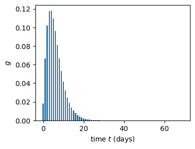
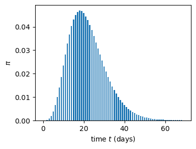
Figure 2: Generating and infection-to-death distributions $g$ and $\pi$ from Bhatt et al., (2020).

In Section 7.1 we illustrate the proposed methods and check their statistical validity using simulated data, then in Section 7.2 we analyze the effect of a mobility measure on the Covid-19 death data used in Bonvini et al., (2022). Throughout this section, we assume that, in Eq. 4, the generating distribution $g$ and infection-to-death distribution $\pi$ are known and equal to those given in Bhatt et al., (2020); they are shown in Fig. 2. We also assume that the ascertainment rate in Eq. 4 is $\alpha_{t}=0.01$, meaning that the probability of death given infection remains constant during the study period. This assumption is sensible here because the period is short and the number of susceptibles at the beginning of the epidemic was large. The specific value $\alpha_{t}=0.01$ does not have to be particularly accurate because it has no effect on the model parameter estimates – any other value would yield the same estimates; it only has a multiplicative effect on the unknown latent infection values, which are not of primary interest. If $\alpha_{t}$ was thought to vary over a longer study period, a model for $\alpha_{t}$ with a small number of parameters would have to be assumed because there is not enough observed data to estimate $\alpha_{t}$ for every $t$. We focus on a single intervention, so that $A_{t}=(1,A_{1t})$ in Eq. 3, yielding the reproduction number model

$$R_{t}=R(\overline{A}_{t},\beta_{0},\beta_{1})=K\left(1+e^{-(\beta_{0}+\beta_{1}A_{1t})}\right)^{-1}.$$ (14)

The maximum possible transmission rate was assumed to be $K=6.5$, which is the largest value found in the literature (Liu et al.,, 2020). Finally, the seeding period was set to $T_{0}=40$, as described in Section 3.

7.1 Analyses of simulated datasets

To illustrate that the algorithm in Section 3 yields sensible ML estimates, we simulated infection and death processes, $I_{t}$ and $Y_{t}$, $t=1,\ldots 120$, from NB distributions with means specified in Eq. 1 and “number of successes” parameters $r_{I}=100$ for the infection process and $r_{Y}=10$ for the death process, $R_{t}$ in Eq. 14, parameters $(\mu,\beta_{0},\beta_{1})=(\log(100),0,-2.2)$ and time-varying binary interventions $A_{1t}=0$ for $t<30$ and $A_{1t}=1$ for $t\geq 30$. We fitted Eqs. 4 and 14 to the data by ML and using the Bayesian approach in Bhatt et al., (2020), assuming the correct NB model for the deaths $Y_{t}$ but assuming that infections $I_{t}$ were deterministic (see Eq. 4 and discussion therein). For the Bayesian approach, we used a shifted gamma prior with shape $1/6$, scale $1$ and shift $\log(1.05)/6$ for $\beta_{1}$, corresponding to mean $(1+\log(1.05))/6=0.17$ and variance $1/6$, and a $N(0,1/4)$ prior for $\beta_{0}$. The choices above match the model, priors, intervention values and parameter estimates for the EuropeCovid data analysed in Bhatt et al., (2020). Finally, for $\mu$ we used the default prior in the Epidemia package: $e^{\mu}\sim\mathrm{Exp}(e^{-\mu_{o}})$ with $e^{\mu_{o}}\sim\mathrm{Exp}(\lambda)$ and $\lambda=0.03$, so that $\mu$ has prior mean $\log(1/0.03)=1.52$, which is close to the true value $\log(100)=1.6$.

True parameters and simulated data are shown in orange in Fig. 3. Bayesian and ML estimates for $(\mu,\beta_{0},\beta_{1})$ and for the mean infection and death processes are overlaid in blue, together with confidence and credible intervals. All estimates appear reasonable and the confidence/credible intervals cover the true values, but with some notable differences between estimation methods. Next, we conduct a simulation study to evaluate the coverage of these intervals.

Maximum Likelihood Estimation

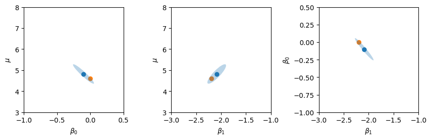
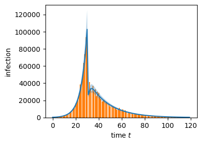
Bayesian Estimation

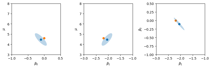
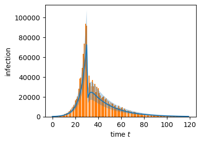
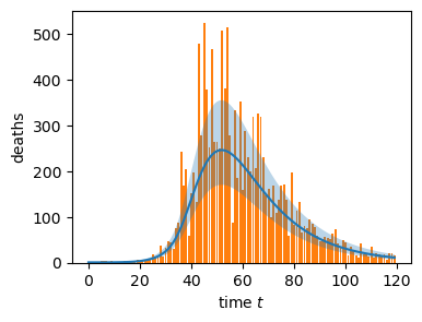
Figure 3: True model parameters, simulated infections and deaths (orange), and overlaid ML and Bayesian estimates (blue), together with 95% confidence/credible intervals (light blue). The infection process in (b,e) and death process in (c,f) were simulated from NB distributions with means in Eq. 1, $R_{t}$ in Eq. 14, true parameters $\mu=\log(100)$, $\beta_{0}=0$ and $\beta_{1}=-2.2$ in (a,d), and binary intervention process $M_{t}=0$ for $t<30$ and $M_{t}=1$ for $t\geq 30$. The model in Eqs. 4 and 14 was fitted assuming NB deaths.

Coverage of ML and Bayesian intervals

Table 1: Coverage study results. Coverages (%) of ML confidence and Bayesian credible intervals for $5$ different values of $(\beta_{0},\beta_{1})$. The true value of $\mu$ was $\log(100)$ in all cases. The priors for $\mu$, $\beta_{0}$ and $\beta_{1}$ were hierarchical exponential, $N(0,1/4)$ and shifted Gamma with mean $0.17$ and variance $1/6$, respectively, as in Bhatt et al., (2020).

$\beta$	(0, -2.2)	(0.25, -2.45)	(0.5, -2.7)	(0.75, -2.95)	(1, -3.2)
ML fit	93.2	95.5	93.7	96.1	95.0
Bhatt et al., (2020)	93.3	95.2	93.6	92.3	84.1

Accurate inference about parameters is important not only to understand, for example, the effect of particular interventions, measured by $\beta_{1}$, but also to produce accurate future predictions of the time course of epidemics, which is one main objective of epidemiological models.

To evaluate the coverage of confidence and credible intervals, we set $(\mu,\beta_{0},\beta_{1})=(\log(100),0,-2.2)$, simulated $1000$ NB infection and death processes as above, fitted the NB model using both ML and Bayesian paradigms with priors as above, and recorded the proportion of times the confidence and credible intervals contained the true parameter. Table 1 contains the resulting empirical 95% coverages; other coverage values gave qualitatively similar results (not shown). We repeated the simulation for four other parameter values. The ML intervals have correct coverage up to simulation error in all cases, whereas the coverage of the Bayesian interval degrades when the prior means of $\beta_{0}$ and $\beta_{1}$, 0 and 0.17 respectively, further deviate from the true values. Note that it is not easy to choose a prior without additional information, as illustrated in Fig. 4, which shows simulated death processes when $(\mu,\beta_{0},\beta_{1})=(\log(100),0,-2.2)$ and $(\mu,\beta_{0},\beta_{1})=(\log(25),1,-3.2)$: all simulated data look very similar and we would be hard pressed to pick different priors for them. It would therefore be wise to select priors that are not too informative.

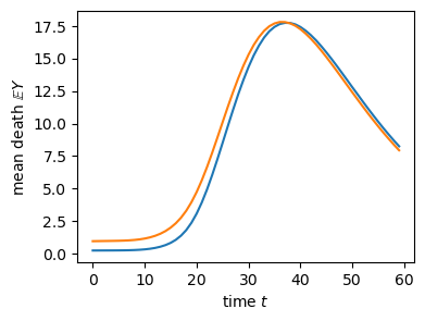
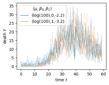
Figure 4: (a) Mean infection and (b) death curves simulated from Eqs. 4 and 14 with $(\mu,\beta_{0},\beta_{1})=(\log(100),0,-2.2)$ (blue) and $(\log(25),1,-3.2)$ (orange), and (c) ten death processes simulated from each of these models, assuming a NB distribution.

Model checking

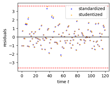
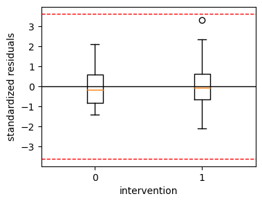
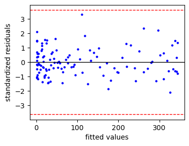
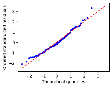
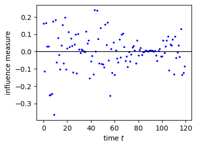
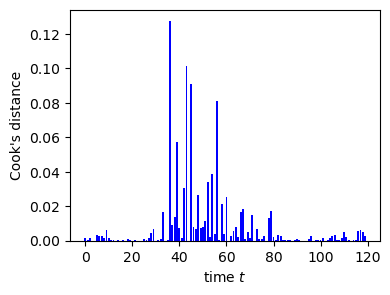
Figure 5: Diagnostics for the NB model fitted to the NB data shown in Fig. 3.

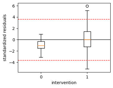
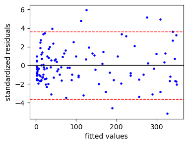
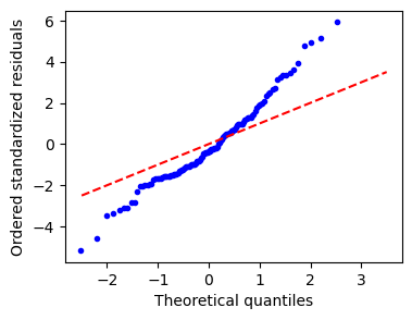
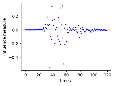
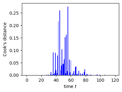
Figure 6: Diagnostics for the Gaussian model fitted to the NB data shown in Fig. 3. (a) Standardized and studentized residuals versus $t$. (b) Standardized residuals versus $A_{t}$ and (c) versus $\widehat{Y}_{t}$. (d) QQ plot of standardized residuals. (e) Influence on $\widehat{\beta}_{1}$ and (f) Cook’s distance, versus $t$.

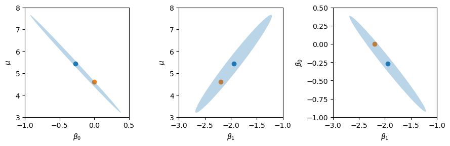
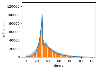
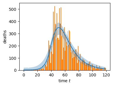
Figure 14: Gaussian model fitted to NB data. True model parameters, simulated infections and deaths (orange); ML and Bayesian estimates (blue) with 95% confidence/credible intervals (light blue). The infection and death processes in (b,c) were simulated from NB distributions with means in Eq. 1, $R_{t}$ in Eq. 14, true parameters $\mu=\log(100)$, $\beta_{0}=0$ and $\beta_{1}=-2.2$ in (a), and binary intervention process $A_{t}=0$ for $t<30$ and $A_{t}=1$ for $t\geq 30$. The model in Eqs. 4 and 14 was fitted assuming Gaussian distributed deaths.

Both ML and Bayesian approaches provide the alternative option of fitting a Gaussian model to the data. Here we illustrate that the standard diagnostics derived from an ML fit can detect model inadequacies. Fig. 5 shows the diagnostics described in Section 4 for the NB model fitted by ML to the simulated NB data shown in Fig. 3. As expected, all diagnostics look fine, since we fit the correct model (except that the model assumes that the latent infection process is deterministic). Fig. 14 in the appendix shows the Gaussian model fitted to the same data and Fig. 6 shows the corresponding diagnostics, where it is clear particularly from panels (b) and (d) that the Gaussian distribution is not a good choice to model the variance of $Y_{t}$. When model diagnostics fail, as is the case in Fig. 6, case diagnostics in (e,f) can look pathological even if there are no outliers or influential observations, so it is best to avoid over-interpreting them.

Shrinkage

Suppose now that we have data from $N=100$ different geographic regions with corresponding parameters $\theta_{i}=(\mu_{i},\beta_{0i},\beta_{1i})$, $i,\ldots,n$. We estimate the $\theta_{i}$’s by maximum likelihood, and take advantage of similarities between the parameters by shrinking the individual estimates towards each other, as described in Section 6. We now evaluate by simulation the coverage of the resulting confidence intervals, for the three following scenarios:

1. $(\mu,\beta_{0},\beta_{1})$ are independent Gaussian random vectors with mean $(\log(300),0,-2)$ and covariance diagonal $(0.5,0.3,0.3)$.

2. $(\beta_{0},\beta_{1})$ are Gaussian vectors with mean $(0,-2)$ and covariance $\begin{pmatrix}0.3&-0.28\\ -0.28&0.3\end{pmatrix}$; $\mu$ is independent of $(\beta_{0},\beta_{1})$ and normally distributed with mean $\log(300)$ and variance $0.5$.

3. $(\mu,\beta_{0},\beta_{1})$ have a mixture distribution with two equal Gaussian components with means $(\log(150),0.5,-2.5)$ and $(\log(600),-0.5,-1.5)$, and covariance matrix $\begin{pmatrix}1&0&0\\ 0&0.5&-0.25\\ 0&-0.25&0.5\end{pmatrix}$ for both components.

The settings in (a), (b) and (c) were chosen so that the marginal means and variances of $\mu$, $\beta_{0}$ and $\beta_{1}$ would be the same, as well as the covariances of $(\beta_{0},\beta_{1})$ in (b) and (c). These choices allowed us to use the same priors in the three scenarios, so coverage differences could not be attributed to difference in priors. We used the hierarchical model of Bhatt et al., (2020):

$$e^{\mu_{i}} \sim\mathrm{Expon}(e^{-\mu^{*}}),$$ (15)

$$\beta_{0i} \sim N(\beta_{0}^{*},\sigma_{0}^{2}),$$

$$\beta_{1i} \sim N(\beta_{1}^{*},\sigma_{1}^{2}),$$

where $(\mu^{*},\beta_{0}^{*},\beta_{1}^{*})$ and $(\mu_{i},\beta_{0i},\beta_{1i})$ denote the global and regional parameters, respectively, with priors and hyper-priors

$$e^{\mu^{*}} \sim\mathrm{Expon}(0.03),$$ (16)

$$\beta_{0}^{*} \sim N(0,1/4), \sigma_{0}\sim\mathrm{Gamma}(2,0.25),$$

$$\beta_{1}^{*} \sim-\log(1.05)/6-\mathrm{Gamma}(1/6,1), \sigma_{1}\sim\mathrm{Gamma}(0.5,0.25).$$

Fig. 9 shows $N=100$ simulated $(\beta_{0},\beta_{1})$ in each scenario, Fig. 9 shows their shrunk ML estimates together with 95% confidence intervals, Fig. 9 shows the corresponding Bayesian estimates, and Table 2 contains the proportion of intervals that contain the true values of $(\mu,\beta_{0},\beta_{1})$. Point and interval estimates are strikingly different across methods, the ML estimates being much closer to the true values. The coverage of the credible intervals also degrades badly as the true dependence structure of the $(\mu_{i},\beta_{0i},\beta_{1i})$ deviates from their assumed independent prior distributions in Eqs. 15 and 16. One could presumably obtain better Bayesian coverage with better priors, although they would be hard to design a priori. On the other hand, ML estimation yields the correct coverage in all cases, up to random error.

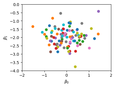
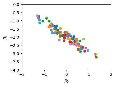
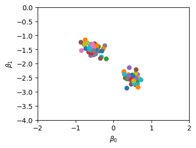
Figure 7: Simultaneous estimation at $N=100$ locations. True $\beta$’s simulated in three scenarios.

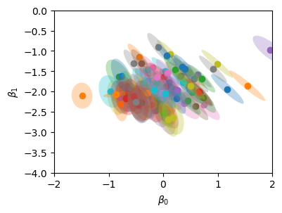
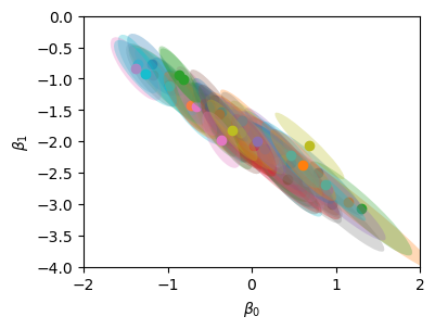
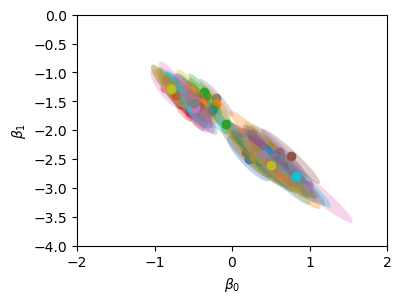
Figure 8: Shrunk ML estimates of $\widehat{\beta}$ and confidence intervals for the true $\beta$’s in Fig. 9.

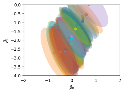
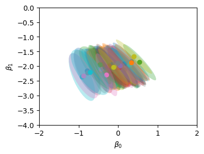
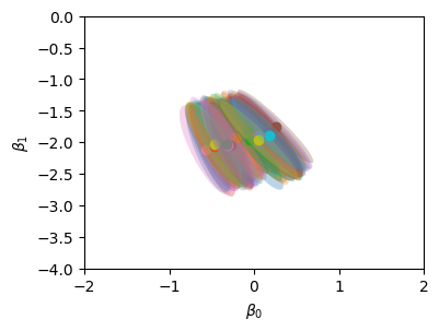
Figure 9: Bayesian estimates and credible intervals for the true $\beta$’s in Fig. 9, using Bhatt et al., (2020).

Table 2: Shrinkage study result. Coverages (%) of ML confidence and Bayesian credible intervals for the three sets of parameters shown in Fig. 9.

Scenario	(a)	(b)	(c)
our method	92	98	95
Bhatt et al., (2020)	91	62	34

7.2 Analysis of Covid-19 time series of deaths in the United States

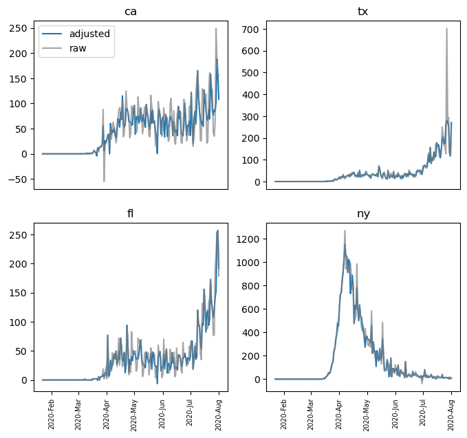
Figure 15: Observed and weekend corrected death time series for four representative states. The large grey spikes lying above the blue curves are the monday effects, and those below are the weekend effects.

We analyzed the effect of a mobility measure on the Covid-19 death data in US states used in Bonvini et al., (2022). The data are from the Delphi repository at Carnegie Mellon University delphi.cmu.edu. The data consist of daily observations, at the state level, on the number of Covid-19 deaths $Y_{t}$ (Fig. 10) and a measure of mobility “proportion at home,” $A_{t}$ (Fig. 16), which is the fraction of mobile devices that spent more than 6 hours at a location other than their home during the daytime (SafeGraph’s full_time_work_behavior_devices/device_count). The time period considered in the analysis was February 15 2020 to August 1 2020. We focused on the $30$ states that reported over 20 deaths on one or more days, and we truncated the time series $30$ days prior to $10$ accumulated deaths, as in Bhatt et al., (2020). This shaved 10 days of data at the start of the period, leaving 156 days of data in each state for analysis, from February 25 to August 1. The death time series showed a strong weekend effect: fewer deaths were reported on saturdays and sundays than one would expect from the numbers reported the previous weeks, and these deaths were instead reported mostly on the following mondays, and tuesdays and wednesdays. Because this effect is not accounted for by the model, it adds variability to the analysis that is due to the reporting process rather than to the epidemic process. For that reason, we pre-processed the data to reduce the effect: for each state, we fitted a nonparametric smooth function to the data together with four additional parameters that estimated the excess Monday, Tuesday and Wednesday effects and deficit saturday effect; we subtracted the estimated effects from all corresponding days and added their sum to all Sundays. Fig. 15 shows the original and adjusted data for four states.

Fig. 10 displays the model ML fits for the 30 states, assuming NB data and regression mean specified in Eqs. 4 and 14. While the overall profiles of the fitted means appear reasonable in all states, in several states there are obvious mismatches between observed and fitted onsets of the pandemic. A possible explanation for this mismatch is a mis-specified infection-to-death distribution $\pi$ in Fig. 2; perhaps $\pi$ should be state specific to account for differences between states, such as different delays in reporting deaths.

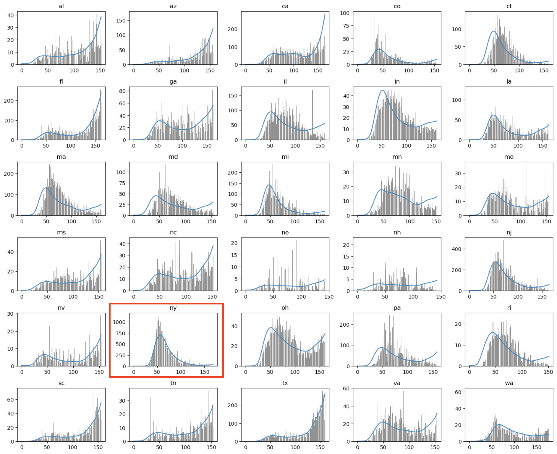
Figure 10: ML fits (blue) to Covid-19 deaths times series in 30 US states for the Feb 15 to August 1st 2020 period. New York is indicated with a box.

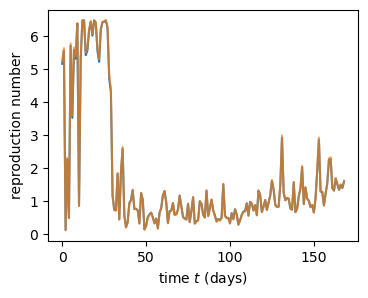
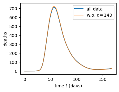
Figure 17: Influence of $Y_{140}$ for NY deaths. (a) Fitted reproduction numbers $R_{t}$ and (b) mean fitted deaths with and without $Y_{140}$. Note that the curves are nearly identical. The data and model fit in NY are in Fig. 10 and diagnostics are in Fig. 12.

Fig. 12 shows model and case diagnostics for the ML fit in NY state. In Fig. 10, there is no apparent onset mismatch in that state but the diagnostics in Fig. 12 clearly shows lack of fit at the start and very end of the epidemic, where all residuals are negative. A more flexible model for $R_{t}$ is needed. The other plots don’t point to egregious other problems other than two outliers in (a), only one of which, at $t=140$, has a very modest influence on the fit: the ML estimates of $(\mu,\beta_{0},\beta_{1})$ are $(2.08,-7.66,14.74)$ and $(2.02,-7.82,15.14)$ with and without that point; the fitted $R_{t}$ and mean death process with and without that point are shown in Appendix Fig. 17. Finally, the seemingly influential points at the end of the range in Fig. 12 are due model lack of fit so are not otherwise suspicious. We also checked the model adequacy in the other states (not shown): apart from the obvious onset mismatches pointed out above, the model and case diagnostics do not raise much concern in most states.

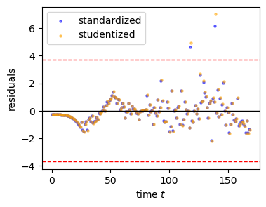
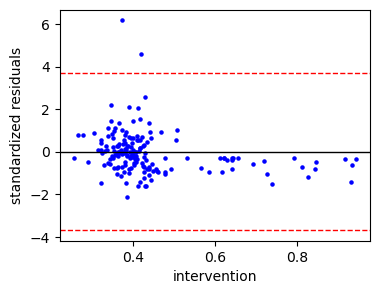
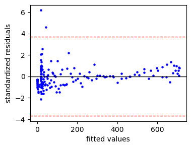
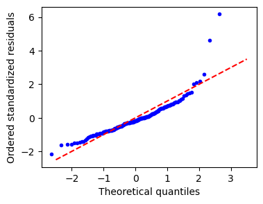
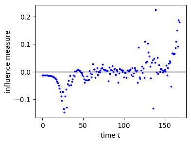
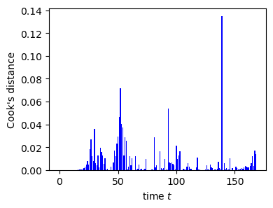
Figure 11: Model diagnostic plots for NY. (a) Standardized and studentized residuals versus $t$. (b) Standardized residuals versus $A_{t}$ and (c) versus $\widehat{Y}_{t}$. The red dashed lines are the $\alpha/2n$ quantiles of the Gaussian distribution. (d) QQ plot of standadized residuals. (e) Studentized residuals versus $t$. (e) Specific influence on $\widehat{\beta}_{1}$ and (f) Cook’s distance versus $t$.

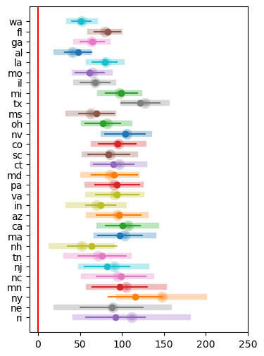
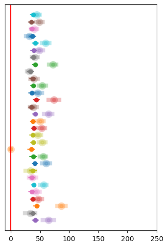
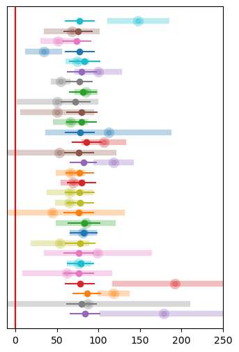
Figure 12: Estimates and confidence intervals for $\beta_{1}$ in Eq. 14 for 30 states using (a) ML, (b) Bhatt et al., (2020) with their priors and (c) with less informative priors. The faint thick lines are the intervals before shrinkage and the dark thin lines after shrinkage. The 30 states are sorted along the y-axis by increasing order of $\operatorname{Var}(\widehat{\beta}_{1})$ before shrinkage.

Fig. 12 displays the ML estimates of $\beta_{1}$ for the 30 states, fitted separately and together using the shrinkage method in Section 6. Fig. 12 displays the Bayesian estimates fitted separately and together, as in Bhatt et al., (2020). Note that we scaled and shifted $A_{t}$ – see Fig. 16 – so that the values would be mostly in the $[0,1]$ range, to match the binary interventions in Bhatt et al., (2020), so we could use their prior distributions. The two estimation methods produce strikingly different inferences: the Bayesian estimates take values in a narrow range around 50 and they have very narrow credible intervals, while the ML estimates have a much larger spread around 100 and their confidence intervals are wider. Clearly, the priors are inappropriate for this data; they are centered on the wrong values and have too small variances. Fig. 12 shows the Bayesian estimates using less informative priors, specifically Eq. 15 with hyper-priors

$$e^{\mu^{*}} \sim\mathrm{Expon}(0.03),$$

$$\beta_{0}^{*} \sim N(0,4), \sigma_{0}\sim\mathrm{Gamma}(1,8),$$

$$\beta_{1}^{*} \sim N(0,4), \sigma_{1}\sim\mathrm{Gamma}(1,8).$$

Now most Bayesian estimates of $\beta_{1}$ take values around 100, which is reassuring since they are closer to the ML estimates. But, ultimately, we have more confidence in the ML estimates given the simulation results in Table 2. Note also that, in some states, the shrunk estimates are drastically different from the marginal estimates, and the credible intervals for the shrunk estimates are rather narrow compared to their un-shrunk counterparts, which may point to some deficiencies of the Bayesian hierarchical model.

Finally, Fig. 13 shows future death predictions and prediction intervals (Section 5) for NY state under two hypothetical trajectory mobility $A_{t}$, based on the shrunk estimates. The Bayesian and ML predictions are strikingly different. We have much more confidence in the latter, although we do not have perfect confidence since the model exhibits some lack of fit, as evidenced in Fig. 12.

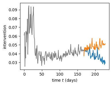
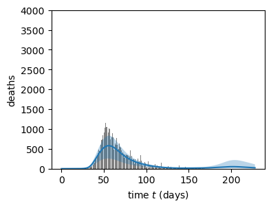
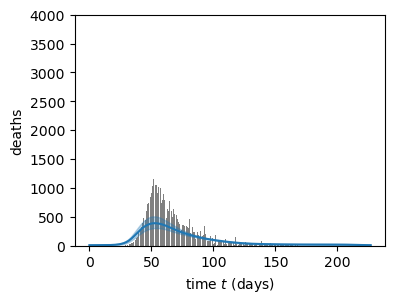
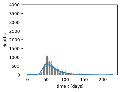
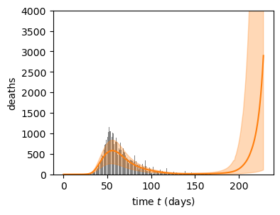
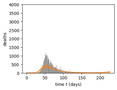
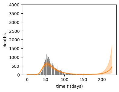
Figure 13: Counterfactual predictions for NY state. (a) Observed intervention when $t\leq 140$ and two, blue and orange, future scenarios ($t\geq 141$). (b,e) Counterfactual mean deaths $\mathbb{E}[Y_{t}]$ with $95\%$ global confidence bands based on the ML based shrinkage estimator (Section 6). (c,f) Corresponding Bayesian predictions using the informative priors in Eqs. 15 and 16, and (d,g) the less informative priors.

8 Discussion

We have discussed statistical inference for a semi-mechanistic epidemic model using frequentist methods. The advantage of using frequentist methods is that there is no need to specify prior distributions and the confidence intervals have valid coverage properties. However, the disadvantage is that these coverage properties are asymptotic in nature in the sense that they hold as the total number of time points $T$ increases.

If the user has informative priors that they want to include then it is possible to do so while preserving frequentist coverage. For example, inverting a test based on the integrated likelihood allows one to include a prior and still have frequentist coverage.

We made simplifying assumptions that are not always reasonable. We assumed $\alpha_{t}=\alpha_{0}$, meaning that the probability that an infected individual produces an outcome (e.g. dies) remains constant over time, which is not reasonable unless the times series are short enough that nothing in the environment changes. Otherwise, changes in virus mutation, medical treatment, season, etc. will affect $\alpha_{t}$. The same argument applies to $R_{t}$. Our model does allow $R_{t}$ to vary with $t$ through $A_{t}$ but a more elaborate model would allow $K$ to also vary with $t$ since, for example, not all variants are as deadly, and part of the population will become immune for a while. One could also use a more flexible model for $R_{t}$, for example by replacing $A_{t}$ with a spline basis evaluated at $A_{t}$. Another improvement would be to let $\pi$ vary by location. Furthermore, one could let $g$ vary with time. All of these generalizations are possible in principle but one has to balance with desire for more complex (and realistic) models with the fact that there is limited information. Informative priors can help but at the cost of losing frequentist coverage properties which is one of the goals of this paper.

The code for the methods in this paper is freely available in our Python package freqepid. Code vignettes we used to generate the results in Section 7 are available at github.com/HeejongBong/freqepid. Inspiration for this project came from the R package Epidemia. Currently, that package implements a wider range of models compared to freqepid but, in principle, the methods there can be extended to provide the same utility as Epidemia. We have found that the models in freqepid often work well even if the generating processes do not match the model.

Appendix A Appendix: Supplementary Figures

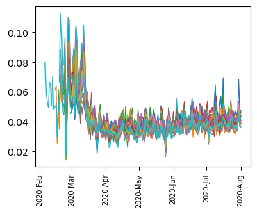
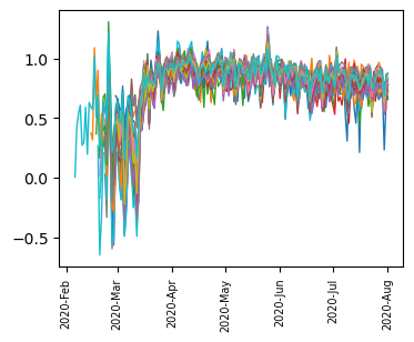
Figure 16: Rescaling and shifting mobility $A_{t}$. (a) Observed Mobility time series in the 30 states and (b) scaled and shifted versions so the new values are mostly in the $[0,1]$ range.

References

- Armstrong et al., (2022) Armstrong, T. B., Kolesár, M., and Plagborg-Møller, M. (2022). Robust empirical bayes confidence intervals. Econometrica, 90(6):2567–2602.
- Baker et al., (2020) Baker, R. E., Park, S. W., Yang, W., Vecchi, G. A., Metcalf, C. J. E., and Grenfell, B. T. (2020). The impact of covid-19 nonpharmaceutical interventions on the future dynamics of endemic infections. Proceedings of the National Academy of Sciences, 117(48):30547–30553.
- Bates et al., (2022) Bates, S., Kennedy, E., Tibshirani, R., Ventura, V., and Wasserman, L. (2022). Causal inference with orthogonalized regression: Taming the phantom. arXiv preprint arXiv:2201.13451.
- Bhatt et al., (2020) Bhatt, S., Ferguson, N., Flaxman, S., Gandy, A., Mishra, S., and Scott, J. A. (2020). Semi-mechanistic bayesian modeling of covid-19 with renewal processes. arXiv preprint arXiv:2012.00394.
- Bonvini et al., (2022) Bonvini, M., Kennedy, E. H., Ventura, V., and Wasserman, L. (2022). Causal inference for the effect of mobility on COVID-19 deaths. The Annals of Applied Statistics, 16(4):2458 – 2480.
- Chatzilena et al., (2019) Chatzilena, A., van Leeuwen, E., Ratmann, O., Baguelin, M., and Demiris, N. (2019). Contemporary statistical inference for infectious disease models using stan. Epidemics, 29:100367.
- Fintzi et al., (2022) Fintzi, J., Wakefield, J., and Minin, V. N. (2022). A linear noise approximation for stochastic epidemic models fit to partially observed incidence counts. Biometrics, 78(4):1530–1541.
- Gunaratne et al., (2022) Gunaratne, C., Reyes, R., Hemberg, E., and O’Reilly, U.-M. (2022). Evaluating efficacy of indoor non-pharmaceutical interventions against covid-19 outbreaks with a coupled spatial-sir agent-based simulation framework. Scientific reports, 12(1):1–11.
- James and Stein, (1992) James, W. and Stein, C. (1992). Estimation with quadratic loss. In Breakthroughs in statistics, pages 443–460. Springer.
- Kermack et al., (1927) Kermack, W. O., McKendrick, A., and Walker, G. T. (1927). A contribution to the mathematical theory of epidemics. Proceedings of the Royal Society of London. Series A, Containing Papers of a Mathematical and Physical Character, 115:700–721.
- Lazebnik et al., (2022) Lazebnik, T., Shami, L., and Bunimovich-Mendrazitsky, S. (2022). Spatio-temporal influence of non-pharmaceutical interventions policies on pandemic dynamics and the economy: the case of covid-19. Economic Research-Ekonomska Istraživanja, 35(1):1833–1861.
- Li et al., (2021) Li, Y. I., Turk, G., Rohrbach, P. B., Pietzonka, P., Kappler, J., Singh, R., Dolezal, J., Ekeh, T., Kikuchi, L., Peterson, J. D., et al. (2021). Efficient bayesian inference of fully stochastic epidemiological models with applications to covid-19. Royal Society Open Science, 8(8):211065.
- Liu et al., (2020) Liu, Y., Gayle, A. A., Wilder-Smith, A., and Rocklöv, J. (2020). The reproductive number of covid-19 is higher compared to sars coronavirus. Journal of travel medicine.
- Morris, (1983) Morris, C. N. (1983). Parametric empirical bayes inference: theory and applications. Journal of the American statistical Association, 78(381):47–55.
- Newey et al., (1987) Newey, W. K., West, K. D., et al. (1987). A simple, positive semi-definite, heteroskedasticity and autocorrelation consistent covariance matrix. Econometrica, 55(3):703–708.
- Perra, (2021) Perra, N. (2021). Non-pharmaceutical interventions during the covid-19 pandemic: A review. Physics Reports, 913:1–52.
- Pötscher and Prucha, (1997) Pötscher, B. M. and Prucha, I. R. (1997). Dynamic Nonlinear Econometric Models: Asymptotic Theory. Springer, Berlin, Heidelberg.
- Robins and Wasserman, (1997) Robins, J. M. and Wasserman, L. A. (1997). Estimation of effects of sequential treatments by reparameterizing directed acyclic graphs. Proceedings of the Thirteenth Conference on Uncertainty in Artificial Intelligence, Providence Rhode Island.
- Scott et al., (2021) Scott, J. A., Gandy, A., Mishra, S., Bhatt, S., Flaxman, S., Unwin, H. J. T., and Ish-Horowicz, J. (2021). Epidemia: an r package for semi-mechanistic bayesian modelling of infectious diseases using point processes. arXiv preprint arXiv:2110.12461.
- Van der Vaart, (2000) Van der Vaart, A. W. (2000). Asymptotic statistics, volume 3. Cambridge university press.
- Vytla et al., (2021) Vytla, V., Ramakuri, S. K., Peddi, A., Srinivas, K. K., and Ragav, N. N. (2021). Mathematical models for predicting covid-19 pandemic: a review. In Journal of Physics: Conference Series, volume 1797, page 012009. IOP Publishing.